Beyond Fierz-Pauli theory - indico.ibs.re.kr · dilaton mode. It is still opened question whether...

Beyond Fierz-Pauli theory

Rampei Kimura Waseda Institue For Advanced Study, Waseda University

COSMO 2018 (Daejeon, Korea)

Collaboration with Daisuke Yamauchi (Kanagawa University) Atsushi Naruko (Tohoku University)

Fierz-Pauli Theory

• Fierz-Pauli theory (Fierz, Pauli, 1939)

gµ⌫ = ⌘µ⌫ + hµ⌫

S = M2Pl

Zd4x

�1

2hµ⌫E↵�

µ⌫ h↵� � 1

4m2(hµ⌫h

µ⌫ � h2)

�

E↵�µ⌫ h↵� = �1

2(⇤hµ⌫ � @µ@↵h

↵⌫ � @⌫@↵h

↵µ + @µ@⌫h

↵↵ � ⌘µ⌫⇤h↵

↵ + ⌘µ⌫@↵@�h↵� )

Only allowed mass term which does not have ghost at linear order

Linearized Einstein-Hilbert term

(1) Lorentz invariant theory(2) No ghost (5 DOF = 2 tensor + 2 vector + 1 scalar)(3) Simple nonlinear extension (massive GR) contains ghost at nonlinear level　 (Boulware-Deser ghost, 6th DOF) (Boulware, Deser, 1971)

Vainshtein screening in quasi-dilaton theory

Rampei Kimura∗

Research Center for the Early Universe (RESCEU),The University of Tokyo, Tokyo, 113-0033, Japan

Gregory Gabadadze†

Center for Cosmology and Particle Physics, Department of Physics,New York University, New York, NY 10003, USA

(Dated: April 1, 2013)

Quasi-dilaton theory is the candidate for massive gravity theory, which couples to an addititonalscalar degrees of freedom. Similarly to dRGT massvie gravity theory, there is no BD ghost in thisthoery. In this paper, we show that there is no usual solution, which posses Vainshtein mechanism.Insted, we only have cosmological solution. We clarly show that assymptotically Minkowski solutionhas always ghost in the scalar modes in the decoupling limit of the theory.

I. INTRODUCTION

It is now belived that general relativity is the theory of gravity, which describe solar system scale and it has beentested for a long decade. It seems that there is no contradiction within tests in our solar system scales. However, ifwe extend this theory to ”cosmology”, we still have a number of question that we can not understand yet. One isthe existance of dark matter, and this is now believed as some particle that we have not discovered yet. Nonethelessthis unknow matter could be of the form of some energy or be part of the theory of gravity. Another example is darkenergy, which is responsible for current cosmic accleration of the universe, and this existance has not confirmed yet.This unknow energy constitues 72 percent of the energy in the universe. One possible solution is the cosmologicalconstant, but this model suffers from the cosmological constant porblem.There might be a chance to explain this cosmic acceleration, for example, modification of gravity or other fluid

that we have not discovered yet. As a candiate of alternative theory of gravity, massive gravity has been recentlyattracted considerable attention. In 1939, Pauli and Fierz found that the ”linearized” massive gravity which doesnot possess ghost. This theory is based on general relativity, and the mass is measured by the difference betweenthe fluctuation of the metric and Minkowski metric. However, Boulwer and Deser found that there is always ghostat nonlienar level. Now we have ghost free massive gravity constructed by de Rham, Gabadadze, and Tolley. Thisincludes all the nonliear terms and describe massive spin-2 particle. Now we have some question whether we can addthe additional scalar model in massive gravity, and this has been done by [] by introducing new symmetry, calledquasi-dilaton theory. This model contains massive spin-2 mode, whose number of degree of freedom is five, and onedilaton mode. It is still opened question whether we have Vainshtein mechanism in this thoery.In this paper, we examine the Vainshtein mechanism in quasi-dilaton theory.

II. THEORY

The action for massive gravity can be described by

SMG =M2

Pl

2

!d4x

√−g

"R− m2

4(U2 + α3U3 + α4U4)

#+ Sm[gµν ,ψ] (1)

where the potential of the massive graviton is given by

U2 = 2εµαρσενβρσKµ

νKαβ = 4

$[K2]− [K]2

%

U3 = εµαγρενβδρKµ

νKαβK

γδ = −[K]3 + 3[K][K2]− 2[K3]

U4 = εµαγρενβδσKµ

νKαβK

γδK

ρσ = −[K]4 + 6[K]2[K2]− 3[K2]2 − 8[K][K3] + 6[K4] (2)

∗Email: rampei"at"theo.phys.sci.hiroshima-u.ac.jp†Email: **"at"**

• dRGT massive gravity (de Rham, Gabadadze, Tolley 2011)

No BD ghost at full order (5 DOF) (Hassan, Rosen, 2011)

Vainshtein screening in quasi-dilaton theory

Rampei Kimura∗

Research Center for the Early Universe (RESCEU),The University of Tokyo, Tokyo, 113-0033, Japan

Gregory Gabadadze†

Center for Cosmology and Particle Physics, Department of Physics,New York University, New York, NY 10003, USA

(Dated: April 9, 2013)

Quasi-dilaton theory is the candidate for massive gravity theory, which couples to an addititonalscalar degrees of freedom. Similarly to dRGT massvie gravity theory, there is no BD ghost in thisthoery. In this paper, we show that there is no usual solution, which posses Vainshtein mechanism.Insted, we only have cosmological solution. We clarly show that assymptotically Minkowski solutionhas always ghost in the scalar modes in the decoupling limit of the theory.

I. INTRODUCTION

It is now belived that general relativity is the theory of gravity, which describe solar system scale and it has beentested for a long decade. It seems that there is no contradiction within tests in our solar system scales. However, ifwe extend this theory to ”cosmology”, we still have a number of question that we can not understand yet. One isthe existance of dark matter, and this is now believed as some particle that we have not discovered yet. Nonethelessthis unknow matter could be of the form of some energy or be part of the theory of gravity. Another example is darkenergy, which is responsible for current cosmic accleration of the universe, and this existance has not confirmed yet.This unknow energy constitues 72 percent of the energy in the universe. One possible solution is the cosmologicalconstant, but this model suffers from the cosmological constant porblem.There might be a chance to explain this cosmic acceleration, for example, modification of gravity or other fluid

that we have not discovered yet. As a candiate of alternative theory of gravity, massive gravity has been recentlyattracted considerable attention. In 1939, Pauli and Fierz found that the ”linearized” massive gravity which doesnot possess ghost. This theory is based on general relativity, and the mass is measured by the difference betweenthe fluctuation of the metric and Minkowski metric. However, Boulwer and Deser found that there is always ghostat nonlienar level. Now we have ghost free massive gravity constructed by de Rham, Gabadadze, and Tolley. Thisincludes all the nonliear terms and describe massive spin-2 particle. Now we have some question whether we can addthe additional scalar model in massive gravity, and this has been done by [] by introducing new symmetry, calledquasi-dilaton theory. This model contains massive spin-2 mode, whose number of degree of freedom is five, and onedilaton mode. It is still opened question whether we have Vainshtein mechanism in this thoery.In this paper, we examine the Vainshtein mechanism in quasi-dilaton theory.

II. THEORY

The action for massive gravity can be described by

SMG =M2

Pl

2

!d4x

√−g

"R− m2

4(U2 + α3U3 + α4U4)

#+ Sm[gµν ,ψ] (1)

where the potential of the massive graviton is given by

U2 = 2εµαρσενβρσKµ

νKαβ = 4

$[K2]− [K]2

%

U3 = εµαγρενβδρKµ

νKαβK

γδ = −[K]3 + 3[K][K2]− 2[K3]

U4 = εµαγρενβδσKµ

νKαβK

γδK

ρσ = −[K]4 + 6[K]2[K2]− 3[K2]2 − 8[K][K3] + 6[K4] (2)

∗Email: rampei"at"theo.phys.sci.hiroshima-u.ac.jp†Email: **"at"**

U2 = [H2]� [H]2 �1

2([H][H2]� [H3]) +O(H4)

Fierz-Pauli mass term Infinite nonlinear corrections to eliminate BD ghost

• Expanding the square root in the potential term

Kµ⌫ = �

µ⌫ �

p�µ⌫ �H

µ⌫ = �

µ⌫ �

⇣pg�1⌘

⌘µ

⌫pXµ

↵

pX↵

⌫ = Xµ⌫

Hµ⌫ = gµ⌫ � ⌘µ⌫

dRGT Massive Gravity

Non-canonical Kinetic Term (RK & Yamauchi, 2013)

SMG =M2

Pl

2

Zd4x

p�g

R� m2

4(U2 + ↵3U3 + ↵4U4)

�+ Sint + Sm[gµ⌫ , ],

• dRGT mass term is uniquely determined• Is dRGT theory a unique theory describing massive graviton without introducing

other fields ?

Lint �M2Pl

p�g g·· H·· R

····,M

2Pl

p�g H·· H·· R

····, · · ·

M2Pl

p�gr.r. H

·· H

··,M

2Pl

p�gr.r. H

·· H

·· H

··, · · ·

• Candidates for derivative interactions

New Kinetic terms???

• No-go theorem - no derivative interaction cannot be introduced in dRGT theory (de Rham et al. 2013)

Lint �M2Pl

p�g g·· H·· R

····,M

2Pl

p�g H·· H·· R

····, · · ·

M2Pl

p�gr.r. H

·· H

··,M

2Pl

p�gr.r. H

·· H

·· H

··, · · ·

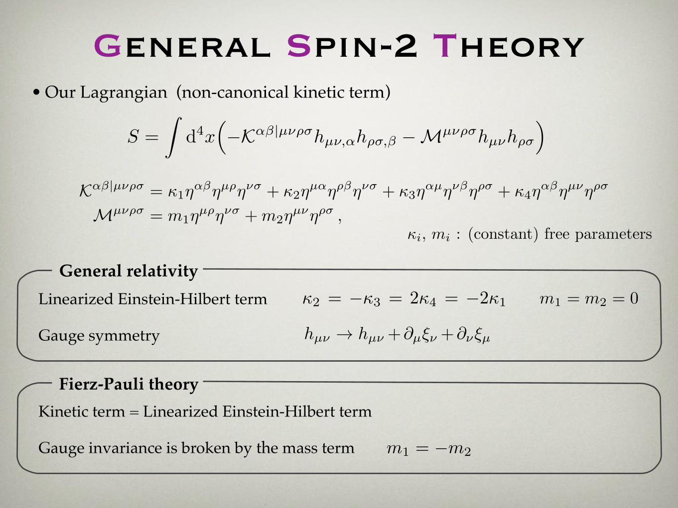
General Spin-2 Theory

2

II. THEORY

A. action

Let us consider a generic action for a spin-2 field hµ⌫ up to the quadratic order in a Minkowski space-time,

S =

Zd4x

⇣�K↵�|µ⌫⇢�

hµ⌫,↵h⇢�,� �Mµ⌫⇢�hµ⌫h⇢�

⌘, (1)

where K↵�|µ⌫⇢� and Mµ⌫⇢� are the most general combination of the Minkowski metric ⌘µ⌫ ,

K↵�|µ⌫⇢� = 1⌘↵�

⌘µ⇢⌘⌫� + 2⌘

µ↵⌘⇢�⌘⌫� + 3⌘

↵µ⌘⌫�⌘⇢� + 4⌘

↵�⌘µ⌫⌘⇢�

, (2)

Mµ⌫⇢� = m1⌘µ⇢⌘⌫� +m2⌘

µ⌫⌘⇢�

, (3)

and 1,2,3,4 and m1,2 are constant parameters. Contracting all the Minkowski metric, the action can be rewritten as

S = �Z

d4xh1hµ⌫ ,↵h

µ⌫ ,↵ + 2h↵µ ,↵h

�µ,� + 3h

↵�,↵h,� + 4h,↵h

,↵ +m1hµ⌫hµ⌫ +m2h

2i, (4)

wherer h is the trace of hµ⌫ contracted with the Minkowski metric ⌘µ⌫ . The linearized Einstein-Hilbert action canbe reproduced by setting 2 = �3 = 24 = �21, and the kinetic term of (1) is then invariant under the gaugetransformation hµ⌫ ! hµ⌫ +@µ⇠⌫ +@⌫⇠µ, where ⇠µ is a gauge parameter. In addition to this choice of the parameters,when the mass parameters satisfy m1 = �m2, the Lagrangian (1) reduces to the Fierz-Pauli theory [1]. Although theFierz-Pauli theory respects the gauge invariance in the kinetic term, it is not neccesary for a massive spin-2 field thatwe consider in the present paper.

B. SVT decomposition

In order to simplify the analysis, we decompose the tensor field hµ⌫ into a transverse-traceless tensor, transversevectors, and scalars :

h00 = h00 = �2↵ , h0i = �h

0i = �,i +Bi (Bi,i = 0) (5)

hij = hij = 2R�ij + 2E,ij + Fi ,j + Fj ,i + 2Hij (F i

,i = 0 , Hii = H

ij,j = 0) . (6)

Here the transverse traceless tensor hij , two transverse vectors Bi and Fi, and four scalars ↵,�,R, and E respectivelyhas two, four, and four components in total. Therefore, to obtain a theory whose degrees of freedom is up to five, weneed to eliminate two (three) components in the vector (scalar) sector. Hereinafter, we, for convenience, work in theFourier space, and the Fourier components of the fields are given by

A(t,x) =

Zd3k

(2⇡)3A(t,k)eik·x , (7)

where A = Hij , Bi, Fi,↵,�,R, or E . Below we split the action into the tensor, vector, and scalar sectors. The actionin the tensor sector is given by

ST = 4

Zdt d3k

h1H

2ij � (1k

2 +m1)H2ij

i, (8)

where a dot represents dervative with respect to time t. The action for the vector modes is given by

SV =

Zdt d3k

h�(21 + 2)B

2i + 21(kFi)

2 + 22kBi(kFi) + 2�1k

2 +m1

�B

2i �

�k2(21 + 2)� 2m1

�(kFi)

2i.

(9)

Finally as for scalar perturbations, the action reduces to

SS =

Zdtd3k

⇣LSkin + LS

cross + LSmass

⌘, (10)

2

II. THEORY

A. action


S =

Zd4x

⇣�K↵�|µ⌫⇢�

hµ⌫,↵h⇢�,� �Mµ⌫⇢�hµ⌫h⇢�

⌘, (1)


K↵�|µ⌫⇢� = 1⌘↵�

⌘µ⇢⌘⌫� + 2⌘

µ↵⌘⇢�⌘⌫� + 3⌘

↵µ⌘⌫�⌘⇢� + 4⌘

↵�⌘µ⌫⌘⇢�

, (2)

Mµ⌫⇢� = m1⌘µ⇢⌘⌫� +m2⌘

µ⌫⌘⇢�

, (3)


S = �Z

d4xh1hµ⌫ ,↵h

µ⌫ ,↵ + 2h↵µ ,↵h

�µ,� + 3h

↵�,↵h,� + 4h,↵h


2i, (4)




h00 = h00 = �2↵ , h0i = �h

0i = �,i +Bi (Bi,i = 0) (5)


,i = 0 , Hii = H

ij,j = 0) . (6)


A(t,x) =

Zd3k

(2⇡)3A(t,k)eik·x , (7)


ST = 4

Zdt d3k

h1H

2ij � (1k

2 +m1)H2ij

i, (8)


SV =

Zdt d3k

h�(21 + 2)B

2i + 21(kFi)

2 + 22kBi(kFi) + 2�1k

2 +m1

�B

2i �

�k2(21 + 2)� 2m1

�(kFi)

2i.

(9)


SS =

Zdtd3k

⇣LSkin + LS

cross + LSmass

⌘, (10)

2

II. THEORY

A. action


S =

Zd4x

⇣�K↵�|µ⌫⇢�

hµ⌫,↵h⇢�,� �Mµ⌫⇢�hµ⌫h⇢�

⌘, (1)


K↵�|µ⌫⇢� = 1⌘↵�

⌘µ⇢⌘⌫� + 2⌘

µ↵⌘⇢�⌘⌫� + 3⌘

↵µ⌘⌫�⌘⇢� + 4⌘

↵�⌘µ⌫⌘⇢�

, (2)

Mµ⌫⇢� = m1⌘µ⇢⌘⌫� +m2⌘

µ⌫⌘⇢�

, (3)


S = �Z

d4xh1hµ⌫ ,↵h

µ⌫ ,↵ + 2h↵µ ,↵h

�µ,� + 3h

↵�,↵h,� + 4h,↵h


2i, (4)




h00 = h00 = �2↵ , h0i = �h

0i = �,i +Bi (Bi,i = 0) (5)


,i = 0 , Hii = H

ij,j = 0) . (6)


A(t,x) =

Zd3k

(2⇡)3A(t,k)eik·x , (7)


ST = 4

Zdt d3k

h1H

2ij � (1k

2 +m1)H2ij

i, (8)


SV =

Zdt d3k

h�(21 + 2)B

2i + 21(kFi)

2 + 22kBi(kFi) + 2�1k

2 +m1

�B

2i �

�k2(21 + 2)� 2m1

�(kFi)

2i.

(9)


SS =

Zdtd3k

⇣LSkin + LS

cross + LSmass

⌘, (10)

2

II. THEORY

A. action


S =

Zd4x

⇣�K↵�|µ⌫⇢�

hµ⌫,↵h⇢�,� �Mµ⌫⇢�hµ⌫h⇢�

⌘, (1)


K↵�|µ⌫⇢� = 1⌘↵�

⌘µ⇢⌘⌫� + 2⌘

µ↵⌘⇢�⌘⌫� + 3⌘

↵µ⌘⌫�⌘⇢� + 4⌘

↵�⌘µ⌫⌘⇢�

, (2)

Mµ⌫⇢� = m1⌘µ⇢⌘⌫� +m2⌘

µ⌫⌘⇢�

, (3)


S = �Z

d4xh1hµ⌫ ,↵h

µ⌫ ,↵ + 2h↵µ ,↵h

�µ,� + 3h

↵�,↵h,� + 4h,↵h


2i, (4)




h00 = h00 = �2↵ , h0i = �h

0i = �,i +Bi (Bi,i = 0) (5)


,i = 0 , Hii = H

ij,j = 0) . (6)


A(t,x) =

Zd3k

(2⇡)3A(t,k)eik·x , (7)


ST = 4

Zdt d3k

h1H

2ij � (1k

2 +m1)H2ij

i, (8)


SV =

Zdt d3k

h�(21 + 2)B

2i + 21(kFi)

2 + 22kBi(kFi) + 2�1k

2 +m1

�B

2i �

�k2(21 + 2)� 2m1

�(kFi)

2i.

(9)


SS =

Zdtd3k

⇣LSkin + LS

cross + LSmass

⌘, (10)

• Our Lagrangian (non-canonical kinetic term)

General relativityLinearized Einstein-Hilbert term

Gauge symmetry

m1 = m2 = 0<latexit sha1_base64="xLWcXiqU4SHMx1rb/buEKAiGr50=">AAACbHichVG7SgNBFD1ZXzE+Eh+FIIIYEqzCXREUISDaWCZqfKASdtdJXLIvdjcBDf6ArYWFWiiIiJ9h4w9Y+Aki2CjYWHizWRAN6h1m5syZe+6cmVEdQ/d8oseI1Nbe0dkV7Y719Pb1xxMDg2ueXXU1UdBsw3Y3VMUThm6Jgq/7hthwXKGYqiHW1cpiY3+9JlxPt61Vf98RO6ZStvSSrik+U5tmUc6axaksFRNJylAQ461ADkESYeTsxDW2sQsbGqowIWDBZ2xAgcdtCzIIDnM7qDPnMtKDfYFDxFhb5SzBGQqzFR7LvNoKWYvXjZpeoNb4FIO7y8pxpOiBbuiV7umWnujj11r1oEbDyz7PalMrnGL8aGTl/V+VybOPvS/Vn559lDAbeNXZuxMwjVtoTX3t4OR1ZW45VU/TJT2z/wt6pDu+gVV7067yYvkUMf4A+edzt4K1qYxMGTk/nZxfCL8iilFMYJLfewbzWEIOBT7XxDHOcB55kYalUWmsmSpFQs0QvoWU/gSHqIx1</latexit><latexit sha1_base64="xLWcXiqU4SHMx1rb/buEKAiGr50=">AAACbHichVG7SgNBFD1ZXzE+Eh+FIIIYEqzCXREUISDaWCZqfKASdtdJXLIvdjcBDf6ArYWFWiiIiJ9h4w9Y+Aki2CjYWHizWRAN6h1m5syZe+6cmVEdQ/d8oseI1Nbe0dkV7Y719Pb1xxMDg2ueXXU1UdBsw3Y3VMUThm6Jgq/7hthwXKGYqiHW1cpiY3+9JlxPt61Vf98RO6ZStvSSrik+U5tmUc6axaksFRNJylAQ461ADkESYeTsxDW2sQsbGqowIWDBZ2xAgcdtCzIIDnM7qDPnMtKDfYFDxFhb5SzBGQqzFR7LvNoKWYvXjZpeoNb4FIO7y8pxpOiBbuiV7umWnujj11r1oEbDyz7PalMrnGL8aGTl/V+VybOPvS/Vn559lDAbeNXZuxMwjVtoTX3t4OR1ZW45VU/TJT2z/wt6pDu+gVV7067yYvkUMf4A+edzt4K1qYxMGTk/nZxfCL8iilFMYJLfewbzWEIOBT7XxDHOcB55kYalUWmsmSpFQs0QvoWU/gSHqIx1</latexit><latexit sha1_base64="xLWcXiqU4SHMx1rb/buEKAiGr50=">AAACbHichVG7SgNBFD1ZXzE+Eh+FIIIYEqzCXREUISDaWCZqfKASdtdJXLIvdjcBDf6ArYWFWiiIiJ9h4w9Y+Aki2CjYWHizWRAN6h1m5syZe+6cmVEdQ/d8oseI1Nbe0dkV7Y719Pb1xxMDg2ueXXU1UdBsw3Y3VMUThm6Jgq/7hthwXKGYqiHW1cpiY3+9JlxPt61Vf98RO6ZStvSSrik+U5tmUc6axaksFRNJylAQ461ADkESYeTsxDW2sQsbGqowIWDBZ2xAgcdtCzIIDnM7qDPnMtKDfYFDxFhb5SzBGQqzFR7LvNoKWYvXjZpeoNb4FIO7y8pxpOiBbuiV7umWnujj11r1oEbDyz7PalMrnGL8aGTl/V+VybOPvS/Vn559lDAbeNXZuxMwjVtoTX3t4OR1ZW45VU/TJT2z/wt6pDu+gVV7067yYvkUMf4A+edzt4K1qYxMGTk/nZxfCL8iilFMYJLfewbzWEIOBT7XxDHOcB55kYalUWmsmSpFQs0QvoWU/gSHqIx1</latexit><latexit sha1_base64="xLWcXiqU4SHMx1rb/buEKAiGr50=">AAACbHichVG7SgNBFD1ZXzE+Eh+FIIIYEqzCXREUISDaWCZqfKASdtdJXLIvdjcBDf6ArYWFWiiIiJ9h4w9Y+Aki2CjYWHizWRAN6h1m5syZe+6cmVEdQ/d8oseI1Nbe0dkV7Y719Pb1xxMDg2ueXXU1UdBsw3Y3VMUThm6Jgq/7hthwXKGYqiHW1cpiY3+9JlxPt61Vf98RO6ZStvSSrik+U5tmUc6axaksFRNJylAQ461ADkESYeTsxDW2sQsbGqowIWDBZ2xAgcdtCzIIDnM7qDPnMtKDfYFDxFhb5SzBGQqzFR7LvNoKWYvXjZpeoNb4FIO7y8pxpOiBbuiV7umWnujj11r1oEbDyz7PalMrnGL8aGTl/V+VybOPvS/Vn559lDAbeNXZuxMwjVtoTX3t4OR1ZW45VU/TJT2z/wt6pDu+gVV7067yYvkUMf4A+edzt4K1qYxMGTk/nZxfCL8iilFMYJLfewbzWEIOBT7XxDHOcB55kYalUWmsmSpFQs0QvoWU/gSHqIx1</latexit>

Fierz-Pauli theoryKinetic term = Linearized Einstein-Hilbert term

Gauge invariance is broken by the mass term

2

II. THEORY

A. action


S =

Zd4x

⇣�K↵�|µ⌫⇢�

hµ⌫,↵h⇢�,� �Mµ⌫⇢�hµ⌫h⇢�

⌘, (1)


K↵�|µ⌫⇢� = 1⌘↵�

⌘µ⇢⌘⌫� + 2⌘

µ↵⌘⇢�⌘⌫� + 3⌘

↵µ⌘⌫�⌘⇢� + 4⌘

↵�⌘µ⌫⌘⇢�

, (2)

Mµ⌫⇢� = m1⌘µ⇢⌘⌫� +m2⌘

µ⌫⌘⇢�

, (3)


S = �Z

d4xh1hµ⌫ ,↵h

µ⌫ ,↵ + 2h↵µ ,↵h

�µ,� + 3h

↵�,↵h,� + 4h,↵h


2i, (4)




h00 = h00 = �2↵ , h0i = �h

0i = �,i +Bi (Bi,i = 0) (5)


,i = 0 , Hii = H

ij,j = 0) . (6)


A(t,x) =

Zd3k

(2⇡)3A(t,k)eik·x , (7)


ST = 4

Zdt d3k

h1H

2ij � (1k

2 +m1)H2ij

i, (8)


SV =

Zdt d3k

h�(21 + 2)B

2i + 21(kFi)

2 + 22kBi(kFi) + 2�1k

2 +m1

�B

2i �

�k2(21 + 2)� 2m1

�(kFi)

2i.

(9)


SS =

Zdtd3k

⇣LSkin + LS

cross + LSmass

⌘, (10)

i, mi : (constant) free parameters<latexit sha1_base64="3psto/qgRmYKyEqeotFJxBMYqA8=">AAACm3ichVHLahRBFD1pX3F8ZEw2ggiNQyRCGG5LiCGrYDYiLvJwkkAmNNXtnaSYfhTVNYPJkB/wB1zoRkFE/AvdCLp1kU8QlxHcuPBOT4NoUG9RVadO3XPrVFVkEl04oqMx79TpM2fPjZ+vXbh46fJE/crkRpH3bMytOE9yuxWpghOdcctpl/CWsazSKOHNqLs83N/ssy10nj10+4Z3UrWb6Y6OlRMqrM+3u8oYFepZvz2bhtpvO37sbDrwF/2ZOM8KpzJ3y+9YZt8oq1J2Uu0wrDeoSWX4J0FQgQaqWMnrr9HGI+SI0UMKRgYnOIFCIW0bAQhGuB0MhLOCdLnPOERNtD3JYslQwnZl3JXVdsVmsh7WLEp1LKck0q0ofUzTZ3pDx/SB3tIX+vHXWoOyxtDLvszRSMsmnHhydf37f1WpzA57v1T/9OzQwULpVYt3UzLDW8Qjff/g6fH64tr04Ca9pK/i/wUd0Xu5Qdb/Fr9a5bVnqMkHBH8+90mwcbsZUDNYnWss3a2+YhzXcAMz8t53sIR7WEFLzn2Od/iIT951b9m77z0YpXpjlWYKv4XX+gloJZ5h</latexit><latexit sha1_base64="3psto/qgRmYKyEqeotFJxBMYqA8=">AAACm3ichVHLahRBFD1pX3F8ZEw2ggiNQyRCGG5LiCGrYDYiLvJwkkAmNNXtnaSYfhTVNYPJkB/wB1zoRkFE/AvdCLp1kU8QlxHcuPBOT4NoUG9RVadO3XPrVFVkEl04oqMx79TpM2fPjZ+vXbh46fJE/crkRpH3bMytOE9yuxWpghOdcctpl/CWsazSKOHNqLs83N/ssy10nj10+4Z3UrWb6Y6OlRMqrM+3u8oYFepZvz2bhtpvO37sbDrwF/2ZOM8KpzJ3y+9YZt8oq1J2Uu0wrDeoSWX4J0FQgQaqWMnrr9HGI+SI0UMKRgYnOIFCIW0bAQhGuB0MhLOCdLnPOERNtD3JYslQwnZl3JXVdsVmsh7WLEp1LKck0q0ofUzTZ3pDx/SB3tIX+vHXWoOyxtDLvszRSMsmnHhydf37f1WpzA57v1T/9OzQwULpVYt3UzLDW8Qjff/g6fH64tr04Ca9pK/i/wUd0Xu5Qdb/Fr9a5bVnqMkHBH8+90mwcbsZUDNYnWss3a2+YhzXcAMz8t53sIR7WEFLzn2Od/iIT951b9m77z0YpXpjlWYKv4XX+gloJZ5h</latexit><latexit sha1_base64="3psto/qgRmYKyEqeotFJxBMYqA8=">AAACm3ichVHLahRBFD1pX3F8ZEw2ggiNQyRCGG5LiCGrYDYiLvJwkkAmNNXtnaSYfhTVNYPJkB/wB1zoRkFE/AvdCLp1kU8QlxHcuPBOT4NoUG9RVadO3XPrVFVkEl04oqMx79TpM2fPjZ+vXbh46fJE/crkRpH3bMytOE9yuxWpghOdcctpl/CWsazSKOHNqLs83N/ssy10nj10+4Z3UrWb6Y6OlRMqrM+3u8oYFepZvz2bhtpvO37sbDrwF/2ZOM8KpzJ3y+9YZt8oq1J2Uu0wrDeoSWX4J0FQgQaqWMnrr9HGI+SI0UMKRgYnOIFCIW0bAQhGuB0MhLOCdLnPOERNtD3JYslQwnZl3JXVdsVmsh7WLEp1LKck0q0ofUzTZ3pDx/SB3tIX+vHXWoOyxtDLvszRSMsmnHhydf37f1WpzA57v1T/9OzQwULpVYt3UzLDW8Qjff/g6fH64tr04Ca9pK/i/wUd0Xu5Qdb/Fr9a5bVnqMkHBH8+90mwcbsZUDNYnWss3a2+YhzXcAMz8t53sIR7WEFLzn2Od/iIT951b9m77z0YpXpjlWYKv4XX+gloJZ5h</latexit><latexit sha1_base64="3psto/qgRmYKyEqeotFJxBMYqA8=">AAACm3ichVHLahRBFD1pX3F8ZEw2ggiNQyRCGG5LiCGrYDYiLvJwkkAmNNXtnaSYfhTVNYPJkB/wB1zoRkFE/AvdCLp1kU8QlxHcuPBOT4NoUG9RVadO3XPrVFVkEl04oqMx79TpM2fPjZ+vXbh46fJE/crkRpH3bMytOE9yuxWpghOdcctpl/CWsazSKOHNqLs83N/ssy10nj10+4Z3UrWb6Y6OlRMqrM+3u8oYFepZvz2bhtpvO37sbDrwF/2ZOM8KpzJ3y+9YZt8oq1J2Uu0wrDeoSWX4J0FQgQaqWMnrr9HGI+SI0UMKRgYnOIFCIW0bAQhGuB0MhLOCdLnPOERNtD3JYslQwnZl3JXVdsVmsh7WLEp1LKck0q0ofUzTZ3pDx/SB3tIX+vHXWoOyxtDLvszRSMsmnHhydf37f1WpzA57v1T/9OzQwULpVYt3UzLDW8Qjff/g6fH64tr04Ca9pK/i/wUd0Xu5Qdb/Fr9a5bVnqMkHBH8+90mwcbsZUDNYnWss3a2+YhzXcAMz8t53sIR7WEFLzn2Od/iIT951b9m77z0YpXpjlWYKv4XX+gloJZ5h</latexit>

Finding Theory

2

II. THEORY

A. action


S =

Zd4x

⇣�K↵�|µ⌫⇢�

hµ⌫,↵h⇢�,� �Mµ⌫⇢�hµ⌫h⇢�

⌘, (1)


K↵�|µ⌫⇢� = 1⌘↵�

⌘µ⇢⌘⌫� + 2⌘

µ↵⌘⇢�⌘⌫� + 3⌘

↵µ⌘⌫�⌘⇢� + 4⌘

↵�⌘µ⌫⌘⇢�

, (2)

Mµ⌫⇢� = m1⌘µ⇢⌘⌫� +m2⌘

µ⌫⌘⇢�

, (3)


S = �Z

d4xh1hµ⌫ ,↵h

µ⌫ ,↵ + 2h↵µ ,↵h

�µ,� + 3h

↵�,↵h,� + 4h,↵h


2i, (4)




h00 = h00 = �2↵ , h0i = �h

0i = �,i +Bi (Bi,i = 0) (5)


,i = 0 , Hii = H

ij,j = 0) . (6)


A(t,x) =

Zd3k

(2⇡)3A(t,k)eik·x , (7)


ST = 4

Zdt d3k

h1H

2ij � (1k

2 +m1)H2ij

i, (8)


SV =

Zdt d3k

h�(21 + 2)B

2i + 21(kFi)

2 + 22kBi(kFi) + 2�1k

2 +m1

�B

2i �

�k2(21 + 2)� 2m1

�(kFi)

2i.

(9)


SS =

Zdtd3k

⇣LSkin + LS

cross + LSmass

⌘, (10)

• SVT decomposition

• Tensor sector

2

II. THEORY

A. action


S =

Zd4x

⇣�K↵�|µ⌫⇢�

hµ⌫,↵h⇢�,� �Mµ⌫⇢�hµ⌫h⇢�

⌘, (1)


K↵�|µ⌫⇢� = 1⌘↵�

⌘µ⇢⌘⌫� + 2⌘

µ↵⌘⇢�⌘⌫� + 3⌘

↵µ⌘⌫�⌘⇢� + 4⌘

↵�⌘µ⌫⌘⇢�

, (2)

Mµ⌫⇢� = m1⌘µ⇢⌘⌫� +m2⌘

µ⌫⌘⇢�

, (3)


S = �Z

d4xh1hµ⌫ ,↵h

µ⌫ ,↵ + 2h↵µ ,↵h

�µ,� + 3h

↵�,↵h,� + 4h,↵h


2i, (4)




h00 = h00 = �2↵ , h0i = �h

0i = �,i +Bi (Bi,i = 0) (5)


,i = 0 , Hii = H

ij,j = 0) . (6)


A(t,x) =

Zd3k

(2⇡)3A(t,k)eik·x , (7)


ST = 4

Zdt d3k

h1H

2ij � (1k

2 +m1)H2ij

i, (8)


SV =

Zdt d3k

h�(21 + 2)B

2i + 21(kFi)

2 + 22kBi(kFi) + 2�1k

2 +m1

�B

2i �

�k2(21 + 2)� 2m1

�(kFi)

2i.

(9)


SS =

Zdtd3k

⇣LSkin + LS

cross + LSmass

⌘, (10)

3

where

LSkin = 4(1 + 2 + 3 + 4)↵

2 � k2(21 + 2)�

2 + 12(1 + 34)R2 + 4(1 + 4)(k2E)2

� 4h�3(3 + 24)R+ (3 + 24)(k

2E)i↵� 8(1 + 34)R(k2E) , (11)

LScross = �4k2

h(2 + 3)↵+ (2 + 33)R� (2 + 3)(k

2E)i� , (12)

LSmass = �4

hk2(1 + 4) +m1 +m2

i↵2 +

hk4(21 + 2) + 2k2m1

i�2

� 4hk2(31 + 2 + 33 + 94) + 3(m1 + 3m2)

iR2 � 4

hk2(1 + 2 + 3 + 4) +m1 +m2

i(k2E)2

� 4h⇣

k2(3 + 64) + 6m2

⌘R�

⇣k2(3 + 24) + 2m2

⌘(k2E)

i↵

+ 8hk2(1 + 2 + 23 + 34) + (m1 + 3m2)

iR(k2E) . (13)

As one can see from (8), the tensor mode is controled by only two parameters 1 and m1, and the existence of tensormode demands

1 6= 0 . (14)

Throughout this paper, we always assume the condition (14), and then the number of the degrees of freedom inthe tensor sector is two. Furthermore, this parameter 1 should be negative 1 > 0 in order for avoiding the ghostinstability in the tensor sector. From the next section, we will investigate the vector and scalar modes in detail.

C. Hamiltonian formalism in Fourier space

In this subsection, we briefly summarize the Hamiltonian formalism in the Fourier space. The Hamiltonian isdefined by

H(t) =

Zd3kH(t,k) , (15)

where H is the Hamiltonian density in the Fourier space,

H(t,k) =X

I

sI(t,k)⇡sI (t,k)� L[sI(t,k), sI(t,k)] , (16)

where sI and ⇡sI are respectively sets of canonical fields and their conjugate momenta. For example, sI = {Bi, Fi}

for the vector field, and sI = {↵,�,R, E}. If the system has n primary constraints Ci, the total Hamiltonian and total

Hamiltonian density are given by

HT (t) =

Zd3kHT (t,k) , HT (t,k) = H(t,k) +

nX

i=1

�i(t,k) Ci(t,k) , (17)

where �i are Lagrange multipliers associated with each primary constraint Ci. The Poisson bracket between A and Bis defined by

{A(t,k),B(t,k0)} =

Zd3k00X

I

�A(t,k)

�sI(t,k00)

�B(t,k0)

�⇡sI (t,k00)� �A(t,k)

�⇡sI (t,k00)

�B(t,k0)

�sI(t,k00)

�. (18)

The time-evolution of the function A(t,k) is given by

A(t,k) = {A(t,k), HT (t)} =

Zd3k0

"{A(t,k),H(t,k0)}+

nX

i=1

�i(t,k0){A(t,k), Ci(t,k0)}

#. (19)

• Ghost-free condition

• Degrees of freedom = 2

Vector Sector

• Bi and Fi has 4 d.o.f → one needs to eliminate one of them (ghost mode)4

III. VECTOR MODES

In this section, we focus on the vector modes and find conditions to avoid appearing extra degrees of freedom, basedon the Hamiltonian analysis. Since the vector has four components, one needs to at least eliminate either Bi or Fi

in order to have two degrees of freedom. The existence of the tensor mode (14) leads to the only option to have aprimary constraint, that is,

21 + 2 = 0 () 2 = �21 . (20)

With this condition (20), the kinetic term of Bi vanishes, which implies Bi manifestly become non-dynamical. Thenthe action for the vector mode can be rewritten with the replacement kFi ! Fi,

SV =

Zdt d3k

h21F

2i � 41kBiFi + 2

�1k

2 �m1

�B

2i � 2m1F

2i

i. (21)

Apparantly, the action for the vector modes depends on only two parameters, 1 and m1, as in the tensor modes.The conjugate momenta for Bi and Fi are given by

⇡Bi = 0 , (22)

⇡Fi = 41(Fi � kBi) , (23)

and we therefore have a primary constraint defined as

CBi1 = ⇡Bi = 0 . (24)

Then Hamiltonian and the total Hamiltonian reads

H = Bi⇡Bi + Fi⇡Fi � L =⇡2Fi

81+ k⇡FiBi � 2m1B

2i + 2m1F

2i ,

HT = H+ �Bi⇡Bi , (25)

where �Bi is a Lagrange multiplier. One can easily check that the evolution of the primary constraint automaticallyyields a secondary constraint,

CBi2 = CBi

1 = {CBi1 , HT } = {CBi

1 , H} = k⇡Fi + 4m1Bi ⇡ 0 . (26)

Then the time-evolution of the secondary constraint is given by1

CBi2 = {CBi

2 , HT } = {CBi2 , H}+ �Bj{C

Bi2 , CBj

1 } ⇡ 0 , (27)

where the coe�cient of �B is given by

{CBi2 , CBj

1 } = 4m1 �ij . (28)

Therefore, we have two cases :Case V1 : m1 6= 0

When m1 6= 0, the last equation can be used to determine the Lagrange multipliers �Bi ,

�Bi ⇡1

4m1{CBi

2 , H} . (29)

Thus, there are two primary constraints CBi1 and two secondary constraints CBi

2 , and all of them are second-class sincethe Poisson bracket between these constraints is non-vanishing. Therefore, the number of the degrees of freedom forthe vector modes is given by

vector DOFs =4⇥ 2� 4 (2 primary & 2 secondary)

2= 2 . (30)

Case V2 : m1 = 0In this case, in addition that the Poisson bracket (29) vanishes, CBi

3 ⌘ {CBi2 , H} also becomes zero. Therefore, there

is no more constraint. Thus there are two primary constraints CBi1 and two secondary constraints CBi

2 , and all of themare first-class since all the Poisson brackets between these constraints vanish. Therefore,

vector DOFs =4⇥ 2� 4 (2 primary & 2 secondary)⇥ 2 (first-class)

2= 0 . (31)

1 To be precise, one needs the integral over the Fourier space in front of the Lagrange multiplier �Bj , which can be always integrablebecause of the appearance of the Dirac’s delta function. For simplicity, we omit this integral and arguments of each variable since resultsdo not change.

4

III. VECTOR MODES



21 + 2 = 0 () 2 = �21 . (20)


SV =

Zdt d3k

h21F

2i � 41kBiFi + 2

�1k

2 �m1

�B

2i � 2m1F

2i

i. (21)


⇡Bi = 0 , (22)

⇡Fi = 41(Fi � kBi) , (23)


CBi1 = ⇡Bi = 0 . (24)




2i + 2m1F

2i ,

HT = H+ �Bi⇡Bi , (25)


CBi2 = CBi

1 = {CBi1 , HT } = {CBi

1 , H} = k⇡Fi + 4m1Bi ⇡ 0 . (26)


CBi2 = {CBi

2 , HT } = {CBi2 , H}+ �Bj{C

Bi2 , CBj

1 } ⇡ 0 , (27)


{CBi2 , CBj

1 } = 4m1 �ij . (28)



�Bi ⇡1

4m1{CBi

2 , H} . (29)




2= 2 . (30)






2= 0 . (31)


• Canonical momenta

4

III. VECTOR MODES



21 + 2 = 0 () 2 = �21 . (20)


SV =

Zdt d3k

h21F

2i � 41kBiFi + 2

�1k

2 �m1

�B

2i � 2m1F

2i

i. (21)


⇡Bi = 0 , (22)

⇡Fi = 41(Fi � kBi) , (23)


CBi1 = ⇡Bi = 0 . (24)




2i + 2m1F

2i ,

HT = H+ �Bi⇡Bi , (25)


CBi2 = CBi

1 = {CBi1 , HT } = {CBi

1 , H} = k⇡Fi + 4m1Bi ⇡ 0 . (26)


CBi2 = {CBi

2 , HT } = {CBi2 , H}+ �Bj{C

Bi2 , CBj

1 } ⇡ 0 , (27)


{CBi2 , CBj

1 } = 4m1 �ij . (28)



�Bi ⇡1

4m1{CBi

2 , H} . (29)




2= 2 . (30)






2= 0 . (31)


4

III. VECTOR MODES



21 + 2 = 0 () 2 = �21 . (20)


SV =

Zdt d3k

h21F

2i � 41kBiFi + 2

�1k

2 �m1

�B

2i � 2m1F

2i

i. (21)


⇡Bi = 0 , (22)

⇡Fi = 41(Fi � kBi) , (23)


CBi1 = ⇡Bi = 0 . (24)




2i + 2m1F

2i ,

HT = H+ �Bi⇡Bi , (25)


CBi2 = CBi

1 = {CBi1 , HT } = {CBi

1 , H} = k⇡Fi + 4m1Bi ⇡ 0 . (26)


CBi2 = {CBi

2 , HT } = {CBi2 , H}+ �Bj{C

Bi2 , CBj

1 } ⇡ 0 , (27)


{CBi2 , CBj

1 } = 4m1 �ij . (28)



�Bi ⇡1

4m1{CBi

2 , H} . (29)




2= 2 . (30)






2= 0 . (31)


Primary constraints

2

II. THEORY

A. action


S =

Zd4x

⇣�K↵�|µ⌫⇢�

hµ⌫,↵h⇢�,� �Mµ⌫⇢�hµ⌫h⇢�

⌘, (1)


K↵�|µ⌫⇢� = 1⌘↵�

⌘µ⇢⌘⌫� + 2⌘

µ↵⌘⇢�⌘⌫� + 3⌘

↵µ⌘⌫�⌘⇢� + 4⌘

↵�⌘µ⌫⌘⇢�

, (2)

Mµ⌫⇢� = m1⌘µ⇢⌘⌫� +m2⌘

µ⌫⌘⇢�

, (3)


S = �Z

d4xh1hµ⌫ ,↵h

µ⌫ ,↵ + 2h↵µ ,↵h

�µ,� + 3h

↵�,↵h,� + 4h,↵h


2i, (4)




h00 = h00 = �2↵ , h0i = �h

0i = �,i +Bi (Bi,i = 0) (5)


,i = 0 , Hii = H

ij,j = 0) . (6)


A(t,x) =

Zd3k

(2⇡)3A(t,k)eik·x , (7)


ST = 4

Zdt d3k

h1H

2ij � (1k

2 +m1)H2ij

i, (8)


SV =

Zdt d3k

h�(21 + 2)B

2i + 21(kFi)

2 + 22kBi(kFi) + 2�1k

2 +m1

�B

2i �

�k2(21 + 2)� 2m1

�(kFi)

2i.

(9)


SS =

Zdtd3k

⇣LSkin + LS

cross + LSmass

⌘, (10)

2

II. THEORY

A. action


S =

Zd4x

⇣�K↵�|µ⌫⇢�

hµ⌫,↵h⇢�,� �Mµ⌫⇢�hµ⌫h⇢�

⌘, (1)


K↵�|µ⌫⇢� = 1⌘↵�

⌘µ⇢⌘⌫� + 2⌘

µ↵⌘⇢�⌘⌫� + 3⌘

↵µ⌘⌫�⌘⇢� + 4⌘

↵�⌘µ⌫⌘⇢�

, (2)

Mµ⌫⇢� = m1⌘µ⇢⌘⌫� +m2⌘

µ⌫⌘⇢�

, (3)


S = �Z

d4xh1hµ⌫ ,↵h

µ⌫ ,↵ + 2h↵µ ,↵h

�µ,� + 3h

↵�,↵h,� + 4h,↵h


2i, (4)




h00 = h00 = �2↵ , h0i = �h

0i = �,i +Bi (Bi,i = 0) (5)


,i = 0 , Hii = H

ij,j = 0) . (6)


A(t,x) =

Zd3k

(2⇡)3A(t,k)eik·x , (7)


ST = 4

Zdt d3k

h1H

2ij � (1k

2 +m1)H2ij

i, (8)


SV =

Zdt d3k

h�(21 + 2)B

2i + 21(kFi)

2 + 22kBi(kFi) + 2�1k

2 +m1

�B

2i �

�k2(21 + 2)� 2m1

�(kFi)

2i.

(9)


SS =

Zdtd3k

⇣LSkin + LS

cross + LSmass

⌘, (10)

4

III. VECTOR MODES



21 + 2 = 0 () 2 = �21 . (20)


SV =

Zdt d3k

h21F

2i � 41kBiFi + 2

�1k

2 �m1

�B

2i � 2m1F

2i

i. (21)


⇡Bi = 0 , (22)

⇡Fi = 41(Fi � kBi) , (23)


CBi1 = ⇡Bi = 0 . (24)




2i + 2m1F

2i ,

HT = H+ �Bi⇡Bi , (25)


CBi2 = CBi

1 = {CBi1 , HT } = {CBi

1 , H} = k⇡Fi + 4m1Bi ⇡ 0 . (26)


CBi2 = {CBi

2 , HT } = {CBi2 , H}+ �Bj{C

Bi2 , CBj

1 } ⇡ 0 , (27)


{CBi2 , CBj

1 } = 4m1 �ij . (28)



�Bi ⇡1

4m1{CBi

2 , H} . (29)




2= 2 . (30)






2= 0 . (31)


4

III. VECTOR MODES



21 + 2 = 0 () 2 = �21 . (20)


SV =

Zdt d3k

h21F

2i � 41kBiFi + 2

�1k

2 �m1

�B

2i � 2m1F

2i

i. (21)


⇡Bi = 0 , (22)

⇡Fi = 41(Fi � kBi) , (23)


CBi1 = ⇡Bi = 0 . (24)




2i + 2m1F

2i ,

HT = H+ �Bi⇡Bi , (25)


CBi2 = CBi

1 = {CBi1 , HT } = {CBi

1 , H} = k⇡Fi + 4m1Bi ⇡ 0 . (26)


CBi2 = {CBi

2 , HT } = {CBi2 , H}+ �Bj{C

Bi2 , CBj

1 } ⇡ 0 , (27)


{CBi2 , CBj

1 } = 4m1 �ij . (28)



�Bi ⇡1

4m1{CBi

2 , H} . (29)




2= 2 . (30)






2= 0 . (31)


4

III. VECTOR MODES



21 + 2 = 0 () 2 = �21 . (20)


SV =

Zdt d3k

h21F

2i � 41kBiFi + 2

�1k

2 �m1

�B

2i � 2m1F

2i

i. (21)


⇡Bi = 0 , (22)

⇡Fi = 41(Fi � kBi) , (23)


CBi1 = ⇡Bi = 0 . (24)




2i + 2m1F

2i ,

HT = H+ �Bi⇡Bi , (25)


CBi2 = CBi

1 = {CBi1 , HT } = {CBi

1 , H} = k⇡Fi + 4m1Bi ⇡ 0 . (26)


CBi2 = {CBi

2 , HT } = {CBi2 , H}+ �Bj{C

Bi2 , CBj

1 } ⇡ 0 , (27)


{CBi2 , CBj

1 } = 4m1 �ij . (28)



�Bi ⇡1

4m1{CBi

2 , H} . (29)




2= 2 . (30)






2= 0 . (31)


• Secondary constraints

• Time-evolution of the secondary constraints

4

III. VECTOR MODES



21 + 2 = 0 () 2 = �21 . (20)


SV =

Zdt d3k

h21F

2i � 41kBiFi + 2

�1k

2 �m1

�B

2i � 2m1F

2i

i. (21)


⇡Bi = 0 , (22)

⇡Fi = 41(Fi � kBi) , (23)


CBi1 = ⇡Bi = 0 . (24)




2i + 2m1F

2i ,

HT = H+ �Bi⇡Bi , (25)


CBi2 = CBi

1 = {CBi1 , HT } = {CBi

1 , H} = k⇡Fi + 4m1Bi ⇡ 0 . (26)


CBi2 = {CBi

2 , HT } = {CBi2 , H}+ �Bj{C

Bi2 , CBj

1 } ⇡ 0 , (27)


{CBi2 , CBj

1 } = 4m1 �ij . (28)



�Bi ⇡1

4m1{CBi

2 , H} . (29)




2= 2 . (30)






2= 0 . (31)


Case 1 :

4

III. VECTOR MODES



21 + 2 = 0 () 2 = �21 . (20)


SV =

Zdt d3k

h21F

2i � 41kBiFi + 2

�1k

2 �m1

�B

2i � 2m1F

2i

i. (21)


⇡Bi = 0 , (22)

⇡Fi = 41(Fi � kBi) , (23)


CBi1 = ⇡Bi = 0 . (24)




2i + 2m1F

2i ,

HT = H+ �Bi⇡Bi , (25)


CBi2 = CBi

1 = {CBi1 , HT } = {CBi

1 , H} = k⇡Fi + 4m1Bi ⇡ 0 . (26)


CBi2 = {CBi

2 , HT } = {CBi2 , H}+ �Bj{C

Bi2 , CBj

1 } ⇡ 0 , (27)


{CBi2 , CBj

1 } = 4m1 �ij . (28)



�Bi ⇡1

4m1{CBi

2 , H} . (29)




2= 2 . (30)






2= 0 . (31)


4

III. VECTOR MODES



21 + 2 = 0 () 2 = �21 . (20)


SV =

Zdt d3k

h21F

2i � 41kBiFi + 2

�1k

2 �m1

�B

2i � 2m1F

2i

i. (21)


⇡Bi = 0 , (22)

⇡Fi = 41(Fi � kBi) , (23)


CBi1 = ⇡Bi = 0 . (24)




2i + 2m1F

2i ,

HT = H+ �Bi⇡Bi , (25)


CBi2 = CBi

1 = {CBi1 , HT } = {CBi

1 , H} = k⇡Fi + 4m1Bi ⇡ 0 . (26)


CBi2 = {CBi

2 , HT } = {CBi2 , H}+ �Bj{C

Bi2 , CBj

1 } ⇡ 0 , (27)


{CBi2 , CBj

1 } = 4m1 �ij . (28)



�Bi ⇡1

4m1{CBi

2 , H} . (29)




2= 2 . (30)






2= 0 . (31)


Case 2 :

4

III. VECTOR MODES



21 + 2 = 0 () 2 = �21 . (20)


SV =

Zdt d3k

h21F

2i � 41kBiFi + 2

�1k

2 �m1

�B

2i � 2m1F

2i

i. (21)


⇡Bi = 0 , (22)

⇡Fi = 41(Fi � kBi) , (23)


CBi1 = ⇡Bi = 0 . (24)




2i + 2m1F

2i ,

HT = H+ �Bi⇡Bi , (25)


CBi2 = CBi

1 = {CBi1 , HT } = {CBi

1 , H} = k⇡Fi + 4m1Bi ⇡ 0 . (26)


CBi2 = {CBi

2 , HT } = {CBi2 , H}+ �Bj{C

Bi2 , CBj

1 } ⇡ 0 , (27)


{CBi2 , CBj

1 } = 4m1 �ij . (28)



�Bi ⇡1

4m1{CBi

2 , H} . (29)




2= 2 . (30)






2= 0 . (31)


Scalar Sector

10

Case S7 : 21 = �2 = 33 = �64, m1 = m2 = 0,If m1 = m2 = 0, both (80) and (81) vanish. In this case, all the primary constraints C�

1 , CR1 and secondary constraints

C�2 , CR

2 are first-class since all the constraints commute with each other. There are two primary constraints C↵1 , C

�1 ,

two secondary constratints C↵2 , C

�2 , and all of them are first-class. Threfore,

scalar DOFs =4⇥ 2� 4 (2 primary & 2 secondary)⇥ 2 (first-class)

2= 0 . (86)

Since the vector modes does not have a degrees of freedom, only the tensor mode propagate. This case is the�21 + 33 = 0 limit of the case S4 as one can see from the structure of the constraint algebra.

Case DOF Conditions Comments

I 3 = 2 + 0 + 1 m1 = 0 & 421 � 413 + 32

3 + 814 6= 0 One primary constraint

II 2 = 2 + 0 + 0 m1 = 0 & 421 � 413 + 32

3 + 814 = 0 Two primary constraints

III 5 = 2 + 2 + 1 m1 6= 0 & 421 � 413 + 32

3 + 814 = 0 New class of 5 DOF theory

& m1(421 � 613 + 32

3) + 4m221 = 0 (Fierz-Pauli is included)

IV 2 = 2 + 0 + 0 m1 = m2 = 0 & 421 � 413 + 32

3 + 814 = 0 general relativity is included

V 2 = 2 + 0 + 0 m1 = 0 & 21 = �2 = 33 = �64 �21 + 33 = 0 limit of case II

VI 5 = 2 + 2 + 1 m1 + 3m2 = 0 & m1 6= 0 & 21 = �2 = 33 = �64 �21 + 33 = 0 limit of case III

VII 2 = 2 + 0 + 0 m1 = m2 = 0 & 21 = �2 = 33 = �64 �21 + 33 = 0 limit of case IV

TABLE I. The number of the degrees of freedom, the conditions for the constant parameters, and comments for each case isshown. For any case, 1 6= 0 and 21 + 2 = 0 are always imposed.


I 3 = 2 + 0 + 1 m1 = 0 & 421 � 413 + 32

3 + 814 6= 0 Partially massless theory

II 2 = 2 + 0 + 0 m1 = 0 & 421 � 413 + 32

3 + 814 = 0 Only tensor modes

III 5 = 2 + 2 + 1 m1 6= 0 & 421 � 413 + 32


& m1(421 � 613 + 32


IV 2 = 2 + 0 + 0 m1 = m2 = 0 Massless limit of case III

& 421 � 413 + 32

3 + 814 = 0 (general relativity is included)

TABLE II. The number of the degrees of freedom, the conditions for the constant parameters, and comments for each case isshown. For any case, 1 6= 0 and 21 + 2 = 0 are always imposed.

V. GAUGE TRANSFORMATION

In this section, we derive a gauge transformation for each case. By using gauge invariant quantities, we also derivea reduced Lagrangian and give conditions for avoiding ghost and gradient instabilities.

A. Case S1

Let us consider the case S1. The generating function is given by the linear combination of the first class constraints,

G = ✏i(t) C�i (87)

Then G = @G/@t+ {G,H} = 0 gives

✏1 + k2✏3 + ✏2 = 0, ✏2 + ✏3 = 0 (88)

This gives

✏1 = ✏� k2✏, ✏2 = �✏, ✏3 = ✏ (89)

• Classification based on the Hamiltonian analysis

• All theories satisfies

• I, II, & IV has gauge symmetries (containing first-class constraints)

• Naive massless limit m1 → 0 of the case III reduces to the case IV, whose

gauge symmetry is given by

10

Case S7 : 21 = �2 = 33 = �64, m1 = m2 = 0,If m1 = m2 = 0, both (80) and (81) vanish. In this case, all the primary constraints C�

1 , CR1 and secondary constraints

C�2 , CR

2 are first-class since all the constraints commute with each other. There are two primary constraints C↵1 , C

�1 ,

two secondary constratints C↵2 , C

�2 , and all of them are first-class. Threfore,

scalar DOFs =4⇥ 2� 4 (2 primary & 2 secondary)⇥ 2 (first-class)

2= 0 . (86)

Since the vector modes does not have a degrees of freedom, only the tensor mode propagate. This case is the�21 + 33 = 0 limit of the case S4 as one can see from the structure of the constraint algebra.


I 3 = 2 + 0 + 1 m1 = 0 & 421 � 413 + 32

3 + 814 6= 0 One primary constraint

II 2 = 2 + 0 + 0 m1 = 0 & 421 � 413 + 32

3 + 814 = 0 Two primary constraints

III 5 = 2 + 2 + 1 m1 6= 0 & 421 � 413 + 32


& m1(421 � 613 + 32


IV 2 = 2 + 0 + 0 m1 = m2 = 0 & 421 � 413 + 32

3 + 814 = 0 general relativity is included

V 2 = 2 + 0 + 0 m1 = 0 & 21 = �2 = 33 = �64 �21 + 33 = 0 limit of case II

VI 5 = 2 + 2 + 1 m1 + 3m2 = 0 & m1 6= 0 & 21 = �2 = 33 = �64 �21 + 33 = 0 limit of case III

VII 2 = 2 + 0 + 0 m1 = m2 = 0 & 21 = �2 = 33 = �64 �21 + 33 = 0 limit of case IV

TABLE I. The number of the degrees of freedom, the conditions for the constant parameters, and comments for each case isshown. For any case, 1 6= 0 and 21 + 2 = 0 are always imposed.


I 3 = 2 + 0 + 1 m1 = 0 & 421 � 413 + 32

3 + 814 6= 0 Partially massless theory

II 2 = 2 + 0 + 0 m1 = 0 & 421 � 413 + 32

3 + 814 = 0 Only tensor modes

III 5 = 2 + 2 + 1 m1 6= 0 & 421 � 413 + 32


& m1(421 � 613 + 32


IV 2 = 2 + 0 + 0 m1 = m2 = 0 Massless limit of case III

& 421 � 413 + 32

3 + 814 = 0 (general relativity is included)

TABLE II. The number of the degrees of freedom, the conditions for the constant parameters, and comments for each case isshown. For any case, 1 6= 0 and 21 + 2 = 0 are always imposed.

V. GAUGE TRANSFORMATION

In this section, we derive a gauge transformation for each case. By using gauge invariant quantities, we also derivea reduced Lagrangian and give conditions for avoiding ghost and gradient instabilities.

A. Case S1

Let us consider the case S1. The generating function is given by the linear combination of the first class constraints,

G = ✏i(t) C�i (87)

Then G = @G/@t+ {G,H} = 0 gives

✏1 + k2✏3 + ✏2 = 0, ✏2 + ✏3 = 0 (88)

This gives

✏1 = ✏� k2✏, ✏2 = �✏, ✏3 = ✏ (89)

hµ⌫ ! hµ⌫ + @µ⇠⌫ + @⌫⇠µ+ b @⇢⇠⇢⌘µ⌫<latexit sha1_base64="75BeR1gsUqPNxmaZpwLYwodRGKY=">AAADBXichVFNb9NAEB0bKMV8NMAFiYtFVISUKBonhSScKrhw7AdpK2WDZbvbZFV/ab2OKFbOSPwBDlwACSGEuCGuHLjwBzj0JyCOReLSQ8eORYAKGMveN2/mjd/uurEvEoW4r+knTp6aOz1/xjh77vyFhcrFSxtJlEqP97zIj+SW6yTcFyHvKaF8vhVL7gSuzzfd3bt5fXPMZSKi8L7ai/kgcIah2BGeo4iyK89HdsaClIXpxDSZisxf8prJYkcq4fg2USZ7KGziTaM2o8OSprKRscJOXw7dQYaNdrfZ6rbq2MBmB1udArSXuu1JjdVdVv85+wGTo2g6pQBcOTMLE8OuVElZhHkcWCWoQhkrUeU1MNiGCDxIIQAOISjCPjiQ0NMHCxBi4gaQEScJiaLOYQIGaVPq4tThELtL3yFl/ZINKc9nJoXao7/49EpSmrCIX/ANHuBnfItf8fCvs7JiRu5lj1Z3quWxvfDkyvqP/6oCWhWMZqp/elawA53CqyDvccHku/Cm+vGjpwfrt9cWs+v4Er+R/xe4j59oB+H4u/dqla89g/wCrD+P+zjYaDYsbFirS9XlO+VVzMNVuAY36LzbsAz3YAV64GlzWl27qd3SH+vv9Pf6h2mrrpWay/Bb6B+PAHNfwVA=</latexit><latexit sha1_base64="75BeR1gsUqPNxmaZpwLYwodRGKY=">AAADBXichVFNb9NAEB0bKMV8NMAFiYtFVISUKBonhSScKrhw7AdpK2WDZbvbZFV/ab2OKFbOSPwBDlwACSGEuCGuHLjwBzj0JyCOReLSQ8eORYAKGMveN2/mjd/uurEvEoW4r+knTp6aOz1/xjh77vyFhcrFSxtJlEqP97zIj+SW6yTcFyHvKaF8vhVL7gSuzzfd3bt5fXPMZSKi8L7ai/kgcIah2BGeo4iyK89HdsaClIXpxDSZisxf8prJYkcq4fg2USZ7KGziTaM2o8OSprKRscJOXw7dQYaNdrfZ6rbq2MBmB1udArSXuu1JjdVdVv85+wGTo2g6pQBcOTMLE8OuVElZhHkcWCWoQhkrUeU1MNiGCDxIIQAOISjCPjiQ0NMHCxBi4gaQEScJiaLOYQIGaVPq4tThELtL3yFl/ZINKc9nJoXao7/49EpSmrCIX/ANHuBnfItf8fCvs7JiRu5lj1Z3quWxvfDkyvqP/6oCWhWMZqp/elawA53CqyDvccHku/Cm+vGjpwfrt9cWs+v4Er+R/xe4j59oB+H4u/dqla89g/wCrD+P+zjYaDYsbFirS9XlO+VVzMNVuAY36LzbsAz3YAV64GlzWl27qd3SH+vv9Pf6h2mrrpWay/Bb6B+PAHNfwVA=</latexit><latexit sha1_base64="75BeR1gsUqPNxmaZpwLYwodRGKY=">AAADBXichVFNb9NAEB0bKMV8NMAFiYtFVISUKBonhSScKrhw7AdpK2WDZbvbZFV/ab2OKFbOSPwBDlwACSGEuCGuHLjwBzj0JyCOReLSQ8eORYAKGMveN2/mjd/uurEvEoW4r+knTp6aOz1/xjh77vyFhcrFSxtJlEqP97zIj+SW6yTcFyHvKaF8vhVL7gSuzzfd3bt5fXPMZSKi8L7ai/kgcIah2BGeo4iyK89HdsaClIXpxDSZisxf8prJYkcq4fg2USZ7KGziTaM2o8OSprKRscJOXw7dQYaNdrfZ6rbq2MBmB1udArSXuu1JjdVdVv85+wGTo2g6pQBcOTMLE8OuVElZhHkcWCWoQhkrUeU1MNiGCDxIIQAOISjCPjiQ0NMHCxBi4gaQEScJiaLOYQIGaVPq4tThELtL3yFl/ZINKc9nJoXao7/49EpSmrCIX/ANHuBnfItf8fCvs7JiRu5lj1Z3quWxvfDkyvqP/6oCWhWMZqp/elawA53CqyDvccHku/Cm+vGjpwfrt9cWs+v4Er+R/xe4j59oB+H4u/dqla89g/wCrD+P+zjYaDYsbFirS9XlO+VVzMNVuAY36LzbsAz3YAV64GlzWl27qd3SH+vv9Pf6h2mrrpWay/Bb6B+PAHNfwVA=</latexit><latexit sha1_base64="75BeR1gsUqPNxmaZpwLYwodRGKY=">AAADBXichVFNb9NAEB0bKMV8NMAFiYtFVISUKBonhSScKrhw7AdpK2WDZbvbZFV/ab2OKFbOSPwBDlwACSGEuCGuHLjwBzj0JyCOReLSQ8eORYAKGMveN2/mjd/uurEvEoW4r+knTp6aOz1/xjh77vyFhcrFSxtJlEqP97zIj+SW6yTcFyHvKaF8vhVL7gSuzzfd3bt5fXPMZSKi8L7ai/kgcIah2BGeo4iyK89HdsaClIXpxDSZisxf8prJYkcq4fg2USZ7KGziTaM2o8OSprKRscJOXw7dQYaNdrfZ6rbq2MBmB1udArSXuu1JjdVdVv85+wGTo2g6pQBcOTMLE8OuVElZhHkcWCWoQhkrUeU1MNiGCDxIIQAOISjCPjiQ0NMHCxBi4gaQEScJiaLOYQIGaVPq4tThELtL3yFl/ZINKc9nJoXao7/49EpSmrCIX/ANHuBnfItf8fCvs7JiRu5lj1Z3quWxvfDkyvqP/6oCWhWMZqp/elawA53CqyDvccHku/Cm+vGjpwfrt9cWs+v4Er+R/xe4j59oB+H4u/dqla89g/wCrD+P+zjYaDYsbFirS9XlO+VVzMNVuAY36LzbsAz3YAV64GlzWl27qd3SH+vv9Pf6h2mrrpWay/Bb6B+PAHNfwVA=</latexit>

12

E. Case S7

The generating function is given by

G =2X

i,j

✏ijCij (103)

where ✏ij is the gauge parameters, and C11 = C�1 , C12 = C�

2 , C21 = CR1 , and C22 = CR

2 . Then, the condition G = 0 givestwo equations,

✏11 + ✏12 + ✏22 = 0, (104)

✏21 + ✏22 + k2✏12 = 0 . (105)

These equations can be recasted into

✏11 = �✏1 � ✏2, ✏12 = ✏1, ✏21 = �k2✏1 � ✏2, ✏22 = ✏2 , (106)

and thus we have two gauge paramaters ✏1 and ✏2. The gauge transformations is given by

�↵ = �k2✏1 , �� = �✏2 � ✏1, (107)

�R = �k2✏1 � ✏2 �E = �k

2✏1 . (108)

One can construct gauge invariant variables as follows,

↵ = ↵� E , R = R� ↵� � +Ek2

(109)

Using these gauge invariant variables, one can show that the reduced Lagrangian becomes zero.

VI. DECOUPLING LIMIT ANALYSIS

Hereafter, we introduce

m1 = c1m2, m2 = c2m

2, (110)

where c1 and c2 are dimensionless constants and m is a mass parameter. One can check that the action of S4 isinvariant under the transformation

hµ⌫ ! hµ⌫ + @µ⇠⌫ + @⌫⇠µ + b @⇢⇠⇢⌘µ⌫ , (111)

up to total derivatives, where the constant b is given by

b = � 21 � 3

2(1 � 3), (112)

Note that b = 0 in GR and Fierz-Pauli theory, and this reproduce the gauge transformation obtained in the previoussection. Now let us consider the Stuckelberg analysis in the case S3. Since the kinetic term of S3 is the same as in thecase S3, we can decompose hµ⌫ by introducing the Stuckelberg fields Aµ (Here, we further decompose Aµ ! Aµ+@µ')as

hµ⌫ = hµ⌫ + @µA⌫ + @⌫Aµ + b @⇢A⇢⌘µ⌫ + 2@µ@⌫'+ b ⌘µ⌫⇤' , (113)

and introduce canonically normalized vector and scalar modes,

Aµ =1

mAµ, ⇡ =

1

m2' . (114)

We then take m ! 0 limit and obtain

L(DL)tensor[h] = �1hµ⌫ ,↵h

µ⌫ ,↵ + 21h↵µ ,↵h

�µ,� � 3h

↵�,↵h,� +

421 � 413 + 32

3

81h,↵h

,↵, (115)

L(DL)scalar�tensor = �c1h

µ⌫

4@µ@⌫⇡ +

(21 � 33)

1⌘µ⌫⇤⇡

�(116)

L(DL)vector = �c1Fµ⌫F

µ⌫ (117)

Decoupling Limit of Case III

• Stuckelberg decomposition

• Decoupling limit

hµ⌫ = hµ⌫ +1

m(@µA⌫ + @⌫Aµ + b @⇢A⇢⌘µ⌫)

<latexit sha1_base64="Jzpdkm14wRM/WB6NNZbaAi8BzrQ=">AAAC+XichVFLaxRBEK4ZX3E17qoXwUuTJZIXS40IiiDEePGYh5sE0nHomXQyTebFTM9CHOYPeBY85JRASNSjP8GLfyCH/ATxGEEQD9bMjm5M0NQw3VXfV19VdbcT+yrViEeGeeHipctXhq42rl0fvtFs3by1mEZZ4squG/lRsuyIVPoqlF2ttC+X40SKwPHlkrP5rOSXejJJVRS+0FuxXA3ERqjWlSs0QXbrjWfnPMh4mBWMPWE594RmXjEAJ1luMR5RDRYUYzwWiVbCt4muk58WNiWyxuSAC09yQck5jE/95l/yxItOJJQRl1r86Tlut9rYwcrYWceqnTbUNhu19oHDGkTgQgYBSAhBk++DgJS+FbAAISZsFXLCEvJUxUsooEHajLIkZQhCN2ndoGilRkOKy5pppXapi09/QkoGo3iI7/AYP+MH/II//1krr2qUs2zR7vS1Mrabr+8sfD9XFdCuwRuo/juzhnV4VM2qaPa4QspTuH1979Xb44XH86P5PdzFrzT/Dh7hJzpB2Pvm7s3J+W1o0ANYp6/7rLN4v2Nhx5p70J6eqZ9iCO7CCIzRfT+EaXgOs9Clvj8MZowbE2Zu7pgH5vt+qmnUmtvwl5kffwF4RcCv</latexit><latexit sha1_base64="Jzpdkm14wRM/WB6NNZbaAi8BzrQ=">AAAC+XichVFLaxRBEK4ZX3E17qoXwUuTJZIXS40IiiDEePGYh5sE0nHomXQyTebFTM9CHOYPeBY85JRASNSjP8GLfyCH/ATxGEEQD9bMjm5M0NQw3VXfV19VdbcT+yrViEeGeeHipctXhq42rl0fvtFs3by1mEZZ4squG/lRsuyIVPoqlF2ttC+X40SKwPHlkrP5rOSXejJJVRS+0FuxXA3ERqjWlSs0QXbrjWfnPMh4mBWMPWE594RmXjEAJ1luMR5RDRYUYzwWiVbCt4muk58WNiWyxuSAC09yQck5jE/95l/yxItOJJQRl1r86Tlut9rYwcrYWceqnTbUNhu19oHDGkTgQgYBSAhBk++DgJS+FbAAISZsFXLCEvJUxUsooEHajLIkZQhCN2ndoGilRkOKy5pppXapi09/QkoGo3iI7/AYP+MH/II//1krr2qUs2zR7vS1Mrabr+8sfD9XFdCuwRuo/juzhnV4VM2qaPa4QspTuH1979Xb44XH86P5PdzFrzT/Dh7hJzpB2Pvm7s3J+W1o0ANYp6/7rLN4v2Nhx5p70J6eqZ9iCO7CCIzRfT+EaXgOs9Clvj8MZowbE2Zu7pgH5vt+qmnUmtvwl5kffwF4RcCv</latexit><latexit sha1_base64="Jzpdkm14wRM/WB6NNZbaAi8BzrQ=">AAAC+XichVFLaxRBEK4ZX3E17qoXwUuTJZIXS40IiiDEePGYh5sE0nHomXQyTebFTM9CHOYPeBY85JRASNSjP8GLfyCH/ATxGEEQD9bMjm5M0NQw3VXfV19VdbcT+yrViEeGeeHipctXhq42rl0fvtFs3by1mEZZ4squG/lRsuyIVPoqlF2ttC+X40SKwPHlkrP5rOSXejJJVRS+0FuxXA3ERqjWlSs0QXbrjWfnPMh4mBWMPWE594RmXjEAJ1luMR5RDRYUYzwWiVbCt4muk58WNiWyxuSAC09yQck5jE/95l/yxItOJJQRl1r86Tlut9rYwcrYWceqnTbUNhu19oHDGkTgQgYBSAhBk++DgJS+FbAAISZsFXLCEvJUxUsooEHajLIkZQhCN2ndoGilRkOKy5pppXapi09/QkoGo3iI7/AYP+MH/II//1krr2qUs2zR7vS1Mrabr+8sfD9XFdCuwRuo/juzhnV4VM2qaPa4QspTuH1979Xb44XH86P5PdzFrzT/Dh7hJzpB2Pvm7s3J+W1o0ANYp6/7rLN4v2Nhx5p70J6eqZ9iCO7CCIzRfT+EaXgOs9Clvj8MZowbE2Zu7pgH5vt+qmnUmtvwl5kffwF4RcCv</latexit><latexit sha1_base64="Jzpdkm14wRM/WB6NNZbaAi8BzrQ=">AAAC+XichVFLaxRBEK4ZX3E17qoXwUuTJZIXS40IiiDEePGYh5sE0nHomXQyTebFTM9CHOYPeBY85JRASNSjP8GLfyCH/ATxGEEQD9bMjm5M0NQw3VXfV19VdbcT+yrViEeGeeHipctXhq42rl0fvtFs3by1mEZZ4squG/lRsuyIVPoqlF2ttC+X40SKwPHlkrP5rOSXejJJVRS+0FuxXA3ERqjWlSs0QXbrjWfnPMh4mBWMPWE594RmXjEAJ1luMR5RDRYUYzwWiVbCt4muk58WNiWyxuSAC09yQck5jE/95l/yxItOJJQRl1r86Tlut9rYwcrYWceqnTbUNhu19oHDGkTgQgYBSAhBk++DgJS+FbAAISZsFXLCEvJUxUsooEHajLIkZQhCN2ndoGilRkOKy5pppXapi09/QkoGo3iI7/AYP+MH/II//1krr2qUs2zR7vS1Mrabr+8sfD9XFdCuwRuo/juzhnV4VM2qaPa4QspTuH1979Xb44XH86P5PdzFrzT/Dh7hJzpB2Pvm7s3J+W1o0ANYp6/7rLN4v2Nhx5p70J6eqZ9iCO7CCIzRfT+EaXgOs9Clvj8MZowbE2Zu7pgH5vt+qmnUmtvwl5kffwF4RcCv</latexit>

m ! 0, M ! 0, T ! 1, ⇤3 andT

Mare fixed

<latexit sha1_base64="A4HcLFrhGPhMyGfl1VydhEHMBuA=">AAACx3ichVFNaxRBEH0Zv+L6kTVeBC+NS8SDLDUqKDkFvSgYyNcmgUxYemZ6kyYz0+NM75J12AWv/gEPnhRExJ+RS/5ADvkJIniJEA8erJ0dEQ1qNd1d73W9qupuP410bokOJ5xTp8+cPTd5vnbh4qXLU/Ur06u56WaBagUmMtm6L3MV6US1rLaRWk8zJWM/Umv+zqPR+VpPZbk2yYrtp2ozlluJ7uhAWqbadT8WnjWCbgvvWVeGYr6CY7RSIk8nHdv/GeE95eyhbN8VhZfFYiiTcDgQBYcaLiTmByU/lJkadvSuCgfteoOaVJo46biV00BlC6b+Hh5CGAToIoZCAst+BImcxwZcEFLmNlEwl7Gny3OFAWqs7XKU4gjJ7A6vW4w2KjZhPMqZl+qAq0Q8M1YKzNABfaAj2qeP9Im+/zVXUeYY9dLn3R9rVdqeenlt+fi/qph3i+1fqn/2bNHBg7JXzb2nJTO6RTDW956/OlqeXZopbtJb+sz9v6FD2uMbJL2vwbtFtfQaNf4A98/nPums3mm61HQX7zXmHlZfMYnruIFb/N73MYfHWECL6+7jC47xzXniGKfn7I5DnYlKcxW/mfPiByAArp8=</latexit><latexit sha1_base64="A4HcLFrhGPhMyGfl1VydhEHMBuA=">AAACx3ichVFNaxRBEH0Zv+L6kTVeBC+NS8SDLDUqKDkFvSgYyNcmgUxYemZ6kyYz0+NM75J12AWv/gEPnhRExJ+RS/5ADvkJIniJEA8erJ0dEQ1qNd1d73W9qupuP410bokOJ5xTp8+cPTd5vnbh4qXLU/Ur06u56WaBagUmMtm6L3MV6US1rLaRWk8zJWM/Umv+zqPR+VpPZbk2yYrtp2ozlluJ7uhAWqbadT8WnjWCbgvvWVeGYr6CY7RSIk8nHdv/GeE95eyhbN8VhZfFYiiTcDgQBYcaLiTmByU/lJkadvSuCgfteoOaVJo46biV00BlC6b+Hh5CGAToIoZCAst+BImcxwZcEFLmNlEwl7Gny3OFAWqs7XKU4gjJ7A6vW4w2KjZhPMqZl+qAq0Q8M1YKzNABfaAj2qeP9Im+/zVXUeYY9dLn3R9rVdqeenlt+fi/qph3i+1fqn/2bNHBg7JXzb2nJTO6RTDW956/OlqeXZopbtJb+sz9v6FD2uMbJL2vwbtFtfQaNf4A98/nPums3mm61HQX7zXmHlZfMYnruIFb/N73MYfHWECL6+7jC47xzXniGKfn7I5DnYlKcxW/mfPiByAArp8=</latexit><latexit sha1_base64="A4HcLFrhGPhMyGfl1VydhEHMBuA=">AAACx3ichVFNaxRBEH0Zv+L6kTVeBC+NS8SDLDUqKDkFvSgYyNcmgUxYemZ6kyYz0+NM75J12AWv/gEPnhRExJ+RS/5ADvkJIniJEA8erJ0dEQ1qNd1d73W9qupuP410bokOJ5xTp8+cPTd5vnbh4qXLU/Ur06u56WaBagUmMtm6L3MV6US1rLaRWk8zJWM/Umv+zqPR+VpPZbk2yYrtp2ozlluJ7uhAWqbadT8WnjWCbgvvWVeGYr6CY7RSIk8nHdv/GeE95eyhbN8VhZfFYiiTcDgQBYcaLiTmByU/lJkadvSuCgfteoOaVJo46biV00BlC6b+Hh5CGAToIoZCAst+BImcxwZcEFLmNlEwl7Gny3OFAWqs7XKU4gjJ7A6vW4w2KjZhPMqZl+qAq0Q8M1YKzNABfaAj2qeP9Im+/zVXUeYY9dLn3R9rVdqeenlt+fi/qph3i+1fqn/2bNHBg7JXzb2nJTO6RTDW956/OlqeXZopbtJb+sz9v6FD2uMbJL2vwbtFtfQaNf4A98/nPums3mm61HQX7zXmHlZfMYnruIFb/N73MYfHWECL6+7jC47xzXniGKfn7I5DnYlKcxW/mfPiByAArp8=</latexit><latexit sha1_base64="A4HcLFrhGPhMyGfl1VydhEHMBuA=">AAACx3ichVFNaxRBEH0Zv+L6kTVeBC+NS8SDLDUqKDkFvSgYyNcmgUxYemZ6kyYz0+NM75J12AWv/gEPnhRExJ+RS/5ADvkJIniJEA8erJ0dEQ1qNd1d73W9qupuP410bokOJ5xTp8+cPTd5vnbh4qXLU/Ur06u56WaBagUmMtm6L3MV6US1rLaRWk8zJWM/Umv+zqPR+VpPZbk2yYrtp2ozlluJ7uhAWqbadT8WnjWCbgvvWVeGYr6CY7RSIk8nHdv/GeE95eyhbN8VhZfFYiiTcDgQBYcaLiTmByU/lJkadvSuCgfteoOaVJo46biV00BlC6b+Hh5CGAToIoZCAst+BImcxwZcEFLmNlEwl7Gny3OFAWqs7XKU4gjJ7A6vW4w2KjZhPMqZl+qAq0Q8M1YKzNABfaAj2qeP9Im+/zVXUeYY9dLn3R9rVdqeenlt+fi/qph3i+1fqn/2bNHBg7JXzb2nJTO6RTDW956/OlqeXZopbtJb+sz9v6FD2uMbJL2vwbtFtfQaNf4A98/nPums3mm61HQX7zXmHlZfMYnruIFb/N73MYfHWECL6+7jC47xzXniGKfn7I5DnYlKcxW/mfPiByAArp8=</latexit>

Aµ = Aµ +1

m@µ⇡

<latexit sha1_base64="MTjs0IBWFZUj69aax8RT+fnYAyQ=">AAAClnichVHNShxBEP6c/OkmxjVehFwGFyUQWGpEMAiKP4geV82q4MjSM/Zq4/wx07ugw76AL+AhpwgikmfwJBhfwIOPIDka8OLB2tmBkIimmu76+qv6qqu7nchTiSa67jJevHz1+k13T+Htu973fcX+D6tJ2IhdWXVDL4zXHZFITwWyqpX25HoUS+E7nlxzdufa8bWmjBMVBl/1XiQ3fbEdqLpyhWaqVrRSe0doc6ZVs/2GOWnOZP6zmVp2yDrTb9mRiLUSXhawI1UrlqhMmZmPgZWDEnKrhMUT2NhCCBcN+JAIoBl7EEh4bMACIWJuEylzMSOVxSVaKLC2wVmSMwSzu7xu824jZwPet2smmdrlUzyeMStNDNMVndItXdIPuqH7J2ulWY12L3vsnY5WRrW+g8GVu/+qfPYaO39Uz/asUceXrFfFvUcZ076F29E39w9vVyaWh9MROqJf3P93uqZzvkHQ/O0eL8nlbyjwB1j/PvdjsDpatqhsLY2Vpmfzr+jGRwzhE7/3OKaxiAqqfO4hznCBn8agMWXMGwudVKMr1wzgLzMqD8izm/A=</latexit><latexit sha1_base64="MTjs0IBWFZUj69aax8RT+fnYAyQ=">AAAClnichVHNShxBEP6c/OkmxjVehFwGFyUQWGpEMAiKP4geV82q4MjSM/Zq4/wx07ugw76AL+AhpwgikmfwJBhfwIOPIDka8OLB2tmBkIimmu76+qv6qqu7nchTiSa67jJevHz1+k13T+Htu973fcX+D6tJ2IhdWXVDL4zXHZFITwWyqpX25HoUS+E7nlxzdufa8bWmjBMVBl/1XiQ3fbEdqLpyhWaqVrRSe0doc6ZVs/2GOWnOZP6zmVp2yDrTb9mRiLUSXhawI1UrlqhMmZmPgZWDEnKrhMUT2NhCCBcN+JAIoBl7EEh4bMACIWJuEylzMSOVxSVaKLC2wVmSMwSzu7xu824jZwPet2smmdrlUzyeMStNDNMVndItXdIPuqH7J2ulWY12L3vsnY5WRrW+g8GVu/+qfPYaO39Uz/asUceXrFfFvUcZ076F29E39w9vVyaWh9MROqJf3P93uqZzvkHQ/O0eL8nlbyjwB1j/PvdjsDpatqhsLY2Vpmfzr+jGRwzhE7/3OKaxiAqqfO4hznCBn8agMWXMGwudVKMr1wzgLzMqD8izm/A=</latexit><latexit sha1_base64="MTjs0IBWFZUj69aax8RT+fnYAyQ=">AAAClnichVHNShxBEP6c/OkmxjVehFwGFyUQWGpEMAiKP4geV82q4MjSM/Zq4/wx07ugw76AL+AhpwgikmfwJBhfwIOPIDka8OLB2tmBkIimmu76+qv6qqu7nchTiSa67jJevHz1+k13T+Htu973fcX+D6tJ2IhdWXVDL4zXHZFITwWyqpX25HoUS+E7nlxzdufa8bWmjBMVBl/1XiQ3fbEdqLpyhWaqVrRSe0doc6ZVs/2GOWnOZP6zmVp2yDrTb9mRiLUSXhawI1UrlqhMmZmPgZWDEnKrhMUT2NhCCBcN+JAIoBl7EEh4bMACIWJuEylzMSOVxSVaKLC2wVmSMwSzu7xu824jZwPet2smmdrlUzyeMStNDNMVndItXdIPuqH7J2ulWY12L3vsnY5WRrW+g8GVu/+qfPYaO39Uz/asUceXrFfFvUcZ076F29E39w9vVyaWh9MROqJf3P93uqZzvkHQ/O0eL8nlbyjwB1j/PvdjsDpatqhsLY2Vpmfzr+jGRwzhE7/3OKaxiAqqfO4hznCBn8agMWXMGwudVKMr1wzgLzMqD8izm/A=</latexit><latexit sha1_base64="MTjs0IBWFZUj69aax8RT+fnYAyQ=">AAAClnichVHNShxBEP6c/OkmxjVehFwGFyUQWGpEMAiKP4geV82q4MjSM/Zq4/wx07ugw76AL+AhpwgikmfwJBhfwIOPIDka8OLB2tmBkIimmu76+qv6qqu7nchTiSa67jJevHz1+k13T+Htu973fcX+D6tJ2IhdWXVDL4zXHZFITwWyqpX25HoUS+E7nlxzdufa8bWmjBMVBl/1XiQ3fbEdqLpyhWaqVrRSe0doc6ZVs/2GOWnOZP6zmVp2yDrTb9mRiLUSXhawI1UrlqhMmZmPgZWDEnKrhMUT2NhCCBcN+JAIoBl7EEh4bMACIWJuEylzMSOVxSVaKLC2wVmSMwSzu7xu824jZwPet2smmdrlUzyeMStNDNMVndItXdIPuqH7J2ulWY12L3vsnY5WRrW+g8GVu/+qfPYaO39Uz/asUceXrFfFvUcZ076F29E39w9vVyaWh9MROqJf3P93uqZzvkHQ/O0eL8nlbyjwB1j/PvdjsDpatqhsLY2Vpmfzr+jGRwzhE7/3OKaxiAqqfO4hznCBn8agMWXMGwudVKMr1wzgLzMqD8izm/A=</latexit>

• Matter coupling

13

where Fµ⌫ = @µA⌫�@⌫Aµ. Here, the self-interaction of the scalar mode does not contribute since it is total derivativesjust as in the case of the Fierz-Pauli case, and the interaction between vector and tensor goes to zero when takingm ! 0. Since the matter Lagrangian is given by

Lmatter =1

Mhµ⌫T

µ⌫, (118)

where Tµ⌫ is the energy-momentum tensor, and M is a mass parameter, which corresponds to the Planck’s mass in

general relativity. Here we have used @µTµ⌫ = 0. In the decoupling limit, the matter sector becomes

L(DL)matter =

1

Mhµ⌫T

µ⌫ +b

⇤33

⇤⇡T (119)

where T = ⌘µ⌫Tµ⌫ and ⇤ = (Mm

2)1/3. Here, we have kept ⇤3 fixed while M ! 1, and the interaction betweenmatter and vector field @

⇢A⇢T goes away since it carries the energy scale ⇤2 = (Mm)1/2. The Lagrangian in the

decoupling limit can be diagonalized by introducing the following conformal transformation,

hµ⌫ = hµ⌫ � c1

1 � 3⇡⌘µ⌫ , (120)

Then the final Lagrangian is given by

L(DL) = L(DL)tensor[h]�

6c11

(@µ⇡)2 +

1

M

hµ⌫T

µ⌫ � c1

1 � 3⇡T

�+

b

⇤33

⇤⇡T , (121)

Thus the equations of motion for ⇡ is given by

12c11

⇤⇡ =1

M

c1

1 � 3T � b

⇤33

⇤T (122)

Probably, there is a ghost degrees of freedom. This is because the matter sector is not invariant under the gaugetransformation that we have found. This implies that the gauge symmetry in the case S4 is immediately broken oncewe introduce the matter Lagrangian.

VII. SUMMARY AND DISCUSSION

In the present paper, we constructed a massive spin-2 field in a flat space-time, whose Lagrangian consists ofthe quadratic terms of the field and its first derivatives. By decomposing the spin-2 field hµ⌫ into the transverse-traceless tensor, transverse vector, and scalar components, we classified theoretically consistent theories based on theHamiltonian analysis in a systematic manner. We found that the existence of the tensor degrees of freedom is alwayscontrolled by one parameter 1, which is assumed to be non-zero although we imposed the degeneracy conditions inorder to eliminate extra degrees of freedom for the vector and scalar modes. Under the degeneracy condition, wefound two classes in the vector sector : 2 propagating vector degrees of freedom and no degrees of freedom. As in thevector sector, we classified theories based on the Hamiltonian anaysis, and found seven classes. One of the classess,with non-vanishing mass terms, is the new theory of a massive spin-2 field where five degrees of freedom propagatein total, and this theory includes the Fierz-Pauli theory. The action of the new theory is given by

S =

Zd4x

"1hµ⌫ ,↵h

µ⌫ ,↵ � 21h↵µ ,↵h

�µ,� + 3h

↵�,↵h,� � 42

1 � 413 + 323

81h,↵h

,↵

+m1

✓hµ⌫h

µ⌫ � 1

421

(421 � 613 + 32

3)h2

◆#, (123)

where 1 6= 0 and m1 6= 0.It is interesting to consider a non-linear extension of our new massive spin-2 theory. Let us consider the following

Lagrangian,

S =

Zd4x

p�g

ha1R+ a2hR+ a3hµ⌫R

µ⌫ + K↵�|µ⌫⇢�r↵hµ⌫r�h⇢� + Mµ⌫⇢�hµ⌫h⇢� +O(h2

R, h3)i, (124)

M : mass dimension parameter (MPl in GR)

m : graviton’s mass (m1 := c1m2)

<latexit sha1_base64="xqccE43WMcg0J4FNJ1glSwIGm7I=">AAAC3HichVHPa9RAFH5J1da1tWu9CF4Gl67byzIpQmWhUPSgl8J267aFpg2TdLoOzUzCzOxqDbl5UrzqwZOCiPhnePEf8NCDf4B4rODFgy/Z4K+ivpB5b7553zffzIRpLIyl9MhxJ06dPjM5dbZ2bnrm/Gz9wtyGSYY64v0oiRO9FTLDY6F43wob861UcybDmG+GBzeL9c0R10Yk6o49TPmOZAMl9kXELEJB/V5zlfiW37daZqRDJDOG7AnJVcEgKdNMcss1aeWrQeZrSbpx/qNfKHKrt5D7fq0pf1UZaDYSNlFXzVgwb8nAI51lEmGSu4sLvh/UG7RNyyAnC68qGlBFN6m/Bh/2IIEIhiCBgwKLdQwMDH7b4AGFFLEdyBDTWIlynUMONeQOsYtjB0P0AMcBzrYrVOG80DQlO8JdYvw1MgnM0w/0DT2m7+lb+ol++6tWVmoUXg4xh2MuT4PZR5fWv/6XJTFbuPuT9U/PFvbheulVoPe0RIpTRGP+6MGz4/VObz5r0pf0M/p/QY/oOzyBGn2JXq3x3nOo4QN4f173yWJjse3Rtrd2rbFyo3qKKbgMV6CF970EK3AbutDHfT86E860M+Puug/dx+6TcavrVJyL8Fu4T78DL3mzUQ==</latexit><latexit sha1_base64="xqccE43WMcg0J4FNJ1glSwIGm7I=">AAAC3HichVHPa9RAFH5J1da1tWu9CF4Gl67byzIpQmWhUPSgl8J267aFpg2TdLoOzUzCzOxqDbl5UrzqwZOCiPhnePEf8NCDf4B4rODFgy/Z4K+ivpB5b7553zffzIRpLIyl9MhxJ06dPjM5dbZ2bnrm/Gz9wtyGSYY64v0oiRO9FTLDY6F43wob861UcybDmG+GBzeL9c0R10Yk6o49TPmOZAMl9kXELEJB/V5zlfiW37daZqRDJDOG7AnJVcEgKdNMcss1aeWrQeZrSbpx/qNfKHKrt5D7fq0pf1UZaDYSNlFXzVgwb8nAI51lEmGSu4sLvh/UG7RNyyAnC68qGlBFN6m/Bh/2IIEIhiCBgwKLdQwMDH7b4AGFFLEdyBDTWIlynUMONeQOsYtjB0P0AMcBzrYrVOG80DQlO8JdYvw1MgnM0w/0DT2m7+lb+ol++6tWVmoUXg4xh2MuT4PZR5fWv/6XJTFbuPuT9U/PFvbheulVoPe0RIpTRGP+6MGz4/VObz5r0pf0M/p/QY/oOzyBGn2JXq3x3nOo4QN4f173yWJjse3Rtrd2rbFyo3qKKbgMV6CF970EK3AbutDHfT86E860M+Puug/dx+6TcavrVJyL8Fu4T78DL3mzUQ==</latexit><latexit sha1_base64="xqccE43WMcg0J4FNJ1glSwIGm7I=">AAAC3HichVHPa9RAFH5J1da1tWu9CF4Gl67byzIpQmWhUPSgl8J267aFpg2TdLoOzUzCzOxqDbl5UrzqwZOCiPhnePEf8NCDf4B4rODFgy/Z4K+ivpB5b7553zffzIRpLIyl9MhxJ06dPjM5dbZ2bnrm/Gz9wtyGSYY64v0oiRO9FTLDY6F43wob861UcybDmG+GBzeL9c0R10Yk6o49TPmOZAMl9kXELEJB/V5zlfiW37daZqRDJDOG7AnJVcEgKdNMcss1aeWrQeZrSbpx/qNfKHKrt5D7fq0pf1UZaDYSNlFXzVgwb8nAI51lEmGSu4sLvh/UG7RNyyAnC68qGlBFN6m/Bh/2IIEIhiCBgwKLdQwMDH7b4AGFFLEdyBDTWIlynUMONeQOsYtjB0P0AMcBzrYrVOG80DQlO8JdYvw1MgnM0w/0DT2m7+lb+ol++6tWVmoUXg4xh2MuT4PZR5fWv/6XJTFbuPuT9U/PFvbheulVoPe0RIpTRGP+6MGz4/VObz5r0pf0M/p/QY/oOzyBGn2JXq3x3nOo4QN4f173yWJjse3Rtrd2rbFyo3qKKbgMV6CF970EK3AbutDHfT86E860M+Puug/dx+6TcavrVJyL8Fu4T78DL3mzUQ==</latexit><latexit sha1_base64="xqccE43WMcg0J4FNJ1glSwIGm7I=">AAAC3HichVHPa9RAFH5J1da1tWu9CF4Gl67byzIpQmWhUPSgl8J267aFpg2TdLoOzUzCzOxqDbl5UrzqwZOCiPhnePEf8NCDf4B4rODFgy/Z4K+ivpB5b7553zffzIRpLIyl9MhxJ06dPjM5dbZ2bnrm/Gz9wtyGSYY64v0oiRO9FTLDY6F43wob861UcybDmG+GBzeL9c0R10Yk6o49TPmOZAMl9kXELEJB/V5zlfiW37daZqRDJDOG7AnJVcEgKdNMcss1aeWrQeZrSbpx/qNfKHKrt5D7fq0pf1UZaDYSNlFXzVgwb8nAI51lEmGSu4sLvh/UG7RNyyAnC68qGlBFN6m/Bh/2IIEIhiCBgwKLdQwMDH7b4AGFFLEdyBDTWIlynUMONeQOsYtjB0P0AMcBzrYrVOG80DQlO8JdYvw1MgnM0w/0DT2m7+lb+ol++6tWVmoUXg4xh2MuT4PZR5fWv/6XJTFbuPuT9U/PFvbheulVoPe0RIpTRGP+6MGz4/VObz5r0pf0M/p/QY/oOzyBGn2JXq3x3nOo4QN4f173yWJjse3Rtrd2rbFyo3qKKbgMV6CF970EK3AbutDHfT86E860M+Puug/dx+6TcavrVJyL8Fu4T78DL3mzUQ==</latexit>

(Massive, DOF=5 case)

13


Lmatter =1

Mhµ⌫T

µ⌫, (118)



L(DL)matter =

1

Mhµ⌫T

µ⌫ +b

⇤33

⇤⇡T (119)





hµ⌫ = hµ⌫ � c1

1 � 3⇡⌘µ⌫ , (120)



6c11

(@µ⇡)2 +

1

M

hµ⌫T

µ⌫ � c1

1 � 3⇡T

�+

b

⇤33

⇤⇡T , (121)


12c11

⇤⇡ =1

M

c1

1 � 3T � b

⇤33

⇤T (122)




S =

Zd4x

"1hµ⌫ ,↵h

µ⌫ ,↵ � 21h↵µ ,↵h

�µ,� + 3h

↵�,↵h,� � 42

1 � 413 + 323

81h,↵h

,↵

+m1

✓hµ⌫h

µ⌫ � 1

421

(421 � 613 + 32

3)h2

◆#, (123)


Lagrangian,

S =

Zd4x

p�g



R, h3)i, (124)

• Matter is also coupled with the second derivatives of ! !

Indicate the presence of higher derivatives ? (in progress)

• New kinetic and mass interactions for spin-2 theories

• 4 independent classes

• Case I : DOF = 3 [2 tensor + 1 scalar] (partially-massless theory)

• Case II : DOF = 2 [2 tensor] (3 first-class, 1 second-class constraints)

• Case III : DOF = 5 [2 tensor + 2 vector + 1 scalar]

• Case IV : DOF = 2 [2 tensor] (4 first-class constraints)

• Matter coupling might be a problem… (need to check !!)

Summary

13


Lmatter =1

Mhµ⌫T

µ⌫, (118)



L(DL)matter =

1

Mhµ⌫T

µ⌫ +b

⇤33

⇤⇡T (119)





hµ⌫ = hµ⌫ � c1

1 � 3⇡⌘µ⌫ , (120)



6c11

(@µ⇡)2 +

1

M

hµ⌫T

µ⌫ � c1

1 � 3⇡T

�+

b

⇤33

⇤⇡T , (121)


12c11

⇤⇡ =1

M

c1

1 � 3T � b

⇤33

⇤T (122)




S =

Zd4x

"1hµ⌫ ,↵h

µ⌫ ,↵ � 21h↵µ ,↵h

�µ,� + 3h

↵�,↵h,� � 42

1 � 413 + 323

81h,↵h

,↵

+m1

✓hµ⌫h

µ⌫ � 1

421

(421 � 613 + 32

3)h2

◆#, (123)


Lagrangian,

S =

Zd4x

p�g



R, h3)i, (124)

Beyond Fierz-Pauli theory - indico.ibs.re.kr · dilaton mode. It is still opened question whether...

Documents

Transcript of Beyond Fierz-Pauli theory - indico.ibs.re.kr · dilaton mode. It is still opened question whether...