1

Best Practices for Fatigue Calculations on FE Models

Presented by:

Dr.-Ing. Stephan Vervoort

Senior Application Engineer Hottinger Baldwin Messtechnik GmbH, nCode Products

2

Agenda

• HBM nCode Products

• Fatigue Analysis Process

• Modeling Recommendations for FE Models

• Defining the Loading Environment

• Defining Material Properties

• Conclusion

3

HBM-nCode Products

• Comprehensive analysis to reporting

• Graphical, interactive & powerful

• World leading fatigue analysis capabilities

• Search, query and reporting data through secure web access

• Analyze, trend and understand using configurable processing

• Powerful fatigue analysis technology

• Integrated reporting and processing

• Fast, expandable, and scalable

Data Processing System for

Engineers

Streamlining the Virtual Fatigue

Engineering Process

Web-based Processing for

Engineering Data

4

A Simple Fatigue Process

5

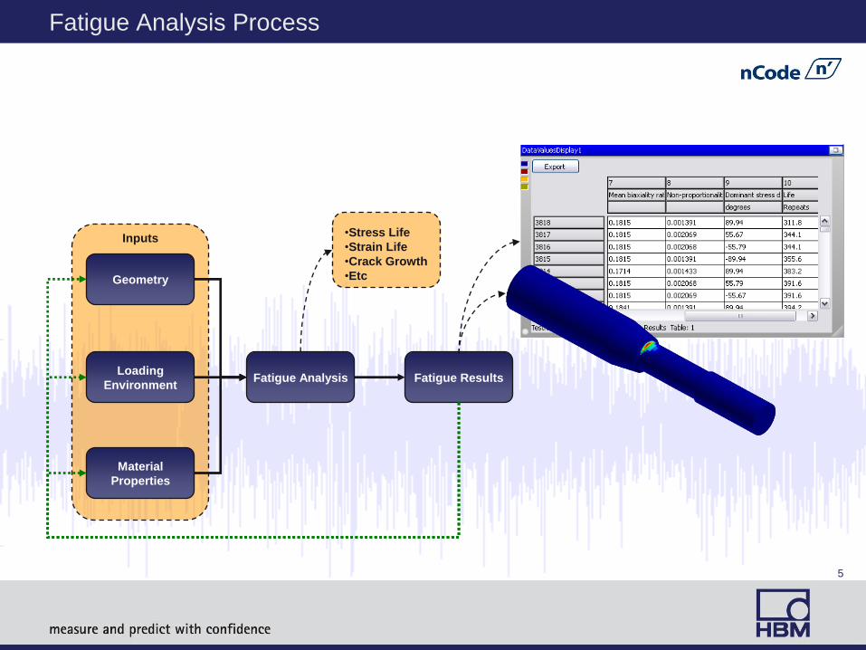
Inputs

Fatigue Analysis Process

Geometry

Loading

Environment

Material

Properties

Fatigue Analysis Fatigue Results

•Stress Life

•Strain Life

•Crack Growth

•Etc

6

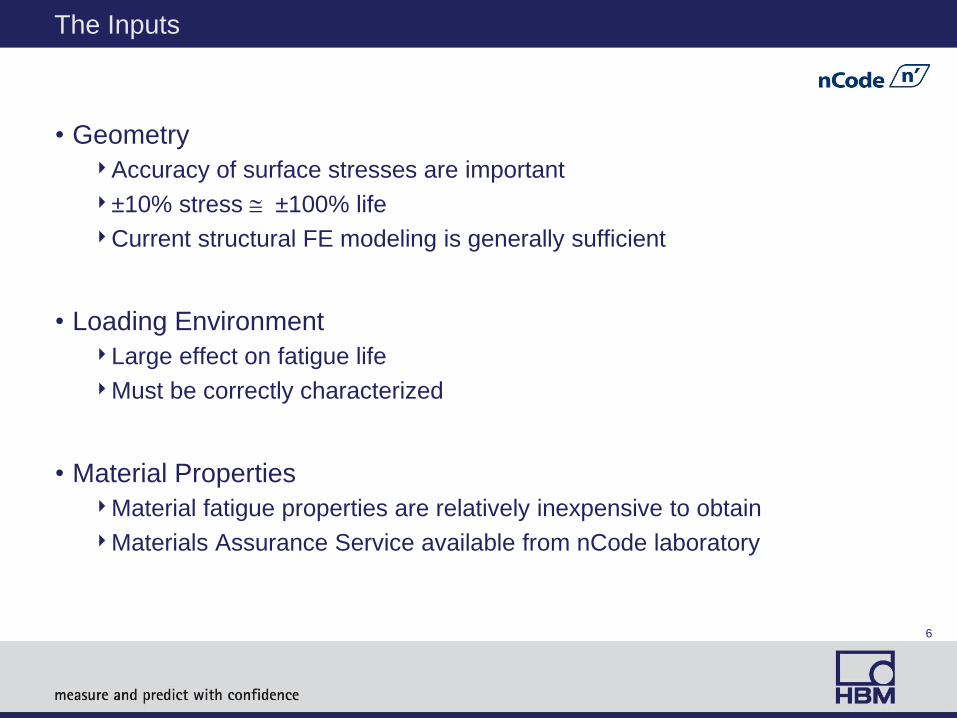
The Inputs

• Geometry

Accuracy of surface stresses are important

±10% stress @ ±100% life

Current structural FE modeling is generally sufficient

• Loading Environment

Large effect on fatigue life

Must be correctly characterized

• Material Properties

Material fatigue properties are relatively inexpensive to obtain

Materials Assurance Service available from nCode laboratory

7

Modeling Recommendations for FE Models

8

Modeling Recommendations for FE Models

• Fatigue cracks usually initiate at free surfaces

• Fatigue damage increases exponentially with stress

±10% stress @ ±100% life

• Recommend using node on element or averaged node on element

Check for convergence

OK for load path &

natural modes

Required for

Fatigue

9

Shell Model

• Stresses calculated at Gauss points and extrapolated to node

• Node has separate stress result from each element

• Most FEA uses average nodal stress

10

Solid Model

• Stresses calculated at Gauss points – but Gauss points are not on surface

• Option 1 – skim surface with membrane or thin shells

Resolves stresses to surface plane

Uses element stresses from the shells as before

• Option 2 – use surface node results

Resolves stresses to the surface

Uses node on element or averaged node on element on surface nodes only

x’

y’

z’

11

Defining the Loading Environment

12

Different Types of Loading Environments

• Linear static superposition

Linear static superposition is an efficient FE analysis technique

This process can also be used for modal superposition

• Time step

Time step is computationally intensive but allows for non-linear analysis and dynamic analysis

• Harmonic response

Harmonic analysis is very efficient for steady state random loading

12

13

Linear Static Superposition

C = FE Stress tensor for Unit

Load Cases

sA

L1=1

L2=1

C1

C2

C1 x

+

=

C2 x

Real Load L1

Real Load L2

Stress time signal at element

14

Modal Superposition

Geometry

Loading

Environment

Material

Properties

Fatigue

Analysis

Fatigue

Results

Modal

Transient

Loading

Histories

Modal Stresses

Modal

Coordinates

SN or EN

Curve

SN or EN

Analysis

Fatigue

Results

L2

L1 L1

L2

f1

f2

s1A* f1(t) + s2A* f2(t) + ... = sA(t)

Mode 1 Mode 2

sA

15

Time Step

Stress for combined loads

calculated by FE point by point

L2

sA L1

L1

L2

For long time histories, issues with solution time

and disk space requirements

Stress time signal at element

Load time signals processed by FE

16

Harmonic Response Transfer Function

C(f) = Complex transfer tensor for

unit Load Cases L(f)

sA

=

Real Load L1

Stress PSD at element

2

C f

C f

1L f

17

Non-linear Contact

L1

L2

Rea

l lo

ad L

1

Rea

l lo

ad L

2

Com

bin

ed l

oad

cas

e

t

t

t

• Non-linear contact is modeled as 2 linear static load cases

• Load cases scaled by real loads

• +ve loads applied to load case 1

• -ve loads applied to load case 2

18

Defining Material Properties

19

• The fatigue life is often described with a single regression curve through data points at which 50% of samples have failed

• More data points result in better confidence, but range of life is also important

• The distribution of points allows for different Certainty of Survival levels

• The distribution of points also allows for the comparison of different batches or supplier

Defining Material Properties

19 4 2 0 2 4 6 8

Supplier A

Supplier B

Supplier A Test Data

Supplier A Regress ion fit

2 s igma range

2 s igma range

Supplier A Des ign curve

Supplier B Tes t Data

SN Fatigue T est Analysis

Number of Cycles to failure N

Str

ess R

ang

e S

20

Conclusion

• Accuracy of damage results depends on accurate surface stresses

• There are three basic types of loading environments

Linear static superposition

Time step

Harmonic response

• Determine if the loading is dynamic or quasi-static

If max frequency in PSD < 1/3 f1 then use static analysis

• The fatigue life curve, certainty of survival, and range of life are all important when characterizing material properties

21

Thanks You

HBM GmbH

nCode Produkte

Carl-Zeiss-Ring 11-13

85737 Ismaning

Tel: +49 (0)89 960537218

Fax: +49 (0)89 960537221

Email: stephan.vervoort@hbmncode.com

www.hbm.com/ncode