Best one-sided approximation to the Heaviside and sign functions

Available online at www.sciencedirect.com

Journal of Approximation Theory 164 (2012) 791–802www.elsevier.com/locate/jat

Full length article

Best one-sided L1 approximation to the Heaviside andsign functions

Jorge Bustamantea, Jose M. Quesadab,∗, Reinaldo Martınez-Cruza

a Fac. Ciencias Fısico Matematicas, B. Universidad Autonoma de Puebla, Av. San Claudio y Rıo Verde, San Manuel,62570 Puebla, Puebla, Mexico

b Departamento de Matematicas, University of Jaen, 23071-Jaen, Spain

Received 4 October 2011; received in revised form 22 January 2012; accepted 22 February 2012Available online 3 March 2012

Communicated by Andras Kroo

Abstract

We find the polynomials of the best one-sided approximation to the Heaviside and sign functions. Thepolynomials are obtained by Hermite interpolation at the zeros of some Jacobi polynomials. Also we givean estimate of the error of approximation and characterize the extremal points of the convex set of the bestapproximants.c⃝ 2012 Elsevier Inc. All rights reserved.

Keywords: One-sided approximation; Jacobi polynomials; Hermite interpolation

1. Introduction

Let Pn denote the family of all algebraic polynomials of degree not greater than n. Forf ∈ L1[−1, 1] bounded from below (above) the error of the best one-sided approximation tof from below (above) of degree n is defined by

E−n ( f )1 = inf ∥ f − P∥1 : P ∈ Pn, P ≤ f E+

n ( f )1 = inf ∥ f − P∥1 : P ∈ Pn, f ≤ P .

∗ Corresponding author.E-mail address: [email protected] (J.M. Quesada).

0021-9045/$ - see front matter c⃝ 2012 Elsevier Inc. All rights reserved.doi:10.1016/j.jat.2012.02.006

http://www.elsevier.com/locate/jat

http://dx.doi.org/10.1016/j.jat.2012.02.006

http://www.elsevier.com/locate/jat

mailto:[email protected]

http://dx.doi.org/10.1016/j.jat.2012.02.006

792 J. Bustamante et al. / Journal of Approximation Theory 164 (2012) 791–802

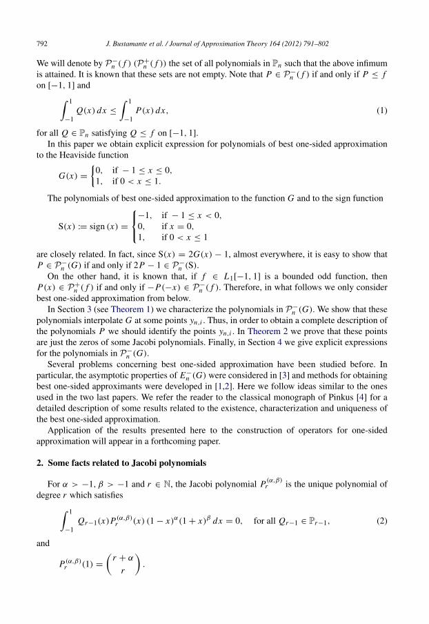
We will denote by P −n ( f ) (P +

n ( f )) the set of all polynomials in Pn such that the above infimumis attained. It is known that these sets are not empty. Note that P ∈ P −

n ( f ) if and only if P ≤ fon [−1, 1] and 1

−1Q(x) dx ≤

1

−1P(x) dx, (1)

for all Q ∈ Pn satisfying Q ≤ f on [−1, 1].In this paper we obtain explicit expression for polynomials of best one-sided approximation

to the Heaviside function

G(x) =

0, if − 1 ≤ x ≤ 0,

1, if 0 < x ≤ 1.

The polynomials of best one-sided approximation to the function G and to the sign function

S(x) := sign (x) =

−1, if − 1 ≤ x < 0,

0, if x = 0,

1, if 0 < x ≤ 1

are closely related. In fact, since S(x) = 2G(x) − 1, almost everywhere, it is easy to show thatP ∈ P −

n (G) if and only if 2P − 1 ∈ P −n (S).

On the other hand, it is known that, if f ∈ L1[−1, 1] is a bounded odd function, thenP(x) ∈ P +

n ( f ) if and only if −P(−x) ∈ P −n ( f ). Therefore, in what follows we only consider

best one-sided approximation from below.In Section 3 (see Theorem 1) we characterize the polynomials in P −

n (G). We show that thesepolynomials interpolate G at some points yn,i . Thus, in order to obtain a complete description ofthe polynomials P we should identify the points yn,i . In Theorem 2 we prove that these pointsare just the zeros of some Jacobi polynomials. Finally, in Section 4 we give explicit expressionsfor the polynomials in P −

n (G).Several problems concerning best one-sided approximation have been studied before. In

particular, the asymptotic properties of E−n (G) were considered in [3] and methods for obtaining

best one-sided approximants were developed in [1,2]. Here we follow ideas similar to the onesused in the two last papers. We refer the reader to the classical monograph of Pinkus [4] for adetailed description of some results related to the existence, characterization and uniqueness ofthe best one-sided approximation.

Application of the results presented here to the construction of operators for one-sidedapproximation will appear in a forthcoming paper.

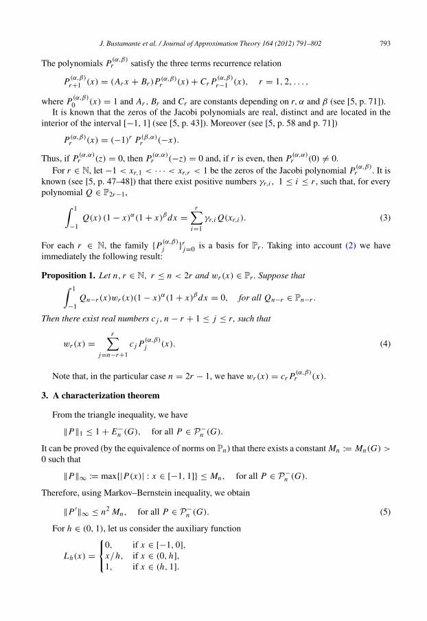
2. Some facts related to Jacobi polynomials

For α > −1, β > −1 and r ∈ N, the Jacobi polynomial P(α,β)r is the unique polynomial of

degree r which satisfies 1

−1Qr−1(x)P(α,β)

r (x) (1 − x)α(1 + x)β dx = 0, for all Qr−1 ∈ Pr−1, (2)

and

P(α,β)r (1) =

r + α

r

.

J. Bustamante et al. / Journal of Approximation Theory 164 (2012) 791–802 793

The polynomials P(α,β)r satisfy the three terms recurrence relation

P(α,β)

r+1 (x) = (Ar x + Br )P(α,β)r (x) + Cr P(α,β)

r−1 (x), r = 1, 2, . . . ,

where P(α,β)

0 (x) = 1 and Ar , Br and Cr are constants depending on r, α and β (see [5, p. 71]).It is known that the zeros of the Jacobi polynomials are real, distinct and are located in the

interior of the interval [−1, 1] (see [5, p. 43]). Moreover (see [5, p. 58 and p. 71])

P(α,β)r (x) = (−1)r P(β,α)

r (−x).

Thus, if P(α,α)r (z) = 0, then P(α,α)

r (−z) = 0 and, if r is even, then P(α,α)r (0) = 0.

For r ∈ N, let −1 < xr,1 < · · · < xr,r < 1 be the zeros of the Jacobi polynomial P(α,β)r . It is

known (see [5, p. 47–48]) that there exist positive numbers γr,i , 1 ≤ i ≤ r , such that, for everypolynomial Q ∈ P2r−1, 1

−1Q(x) (1 − x)α(1 + x)βdx =

ri=1

γr,i Q(xr,i ). (3)

For each r ∈ N, the family P(α,β)j

rj=0 is a basis for Pr . Taking into account (2) we have

immediately the following result:

Proposition 1. Let n, r ∈ N, r ≤ n < 2r and wr (x) ∈ Pr . Suppose that 1

−1Qn−r (x)wr (x)(1 − x)α(1 + x)βdx = 0, for all Qn−r ∈ Pn−r .

Then there exist real numbers c j , n − r + 1 ≤ j ≤ r , such that

wr (x) =

rj=n−r+1

c j P(α,β)j (x). (4)

Note that, in the particular case n = 2r − 1, we have wr (x) = cr P(α,β)r (x).

3. A characterization theorem

From the triangle inequality, we have

∥P∥1 ≤ 1 + E−n (G), for all P ∈ P −

n (G).

It can be proved (by the equivalence of norms on Pn) that there exists a constant Mn := Mn(G) >

0 such that

∥P∥∞ := max|P(x)| : x ∈ [−1, 1] ≤ Mn, for all P ∈ P −n (G).

Therefore, using Markov–Bernstein inequality, we obtain

∥P ′∥∞ ≤ n2 Mn, for all P ∈ P −

n (G). (5)

For h ∈ (0, 1), let us consider the auxiliary function

Lh(x) =

0, if x ∈ [−1, 0],

x/h, if x ∈ (0, h],

1, if x ∈ (h, 1].


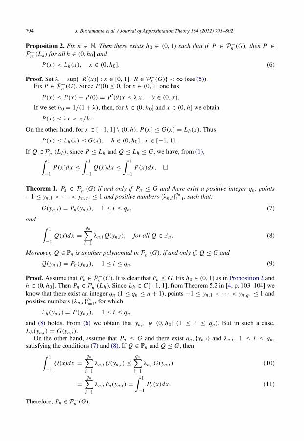
Proposition 2. Fix n ∈ N. Then there exists h0 ∈ (0, 1) such that if P ∈ P −n (G), then P ∈

P −n (Lh) for all h ∈ (0, h0] and

P(x) < Lh(x), x ∈ (0, h0]. (6)

Proof. Set λ = sup |R′(x)| : x ∈ [0, 1], R ∈ P −n (G) < ∞ (see (5)).

Fix P ∈ P −n (G). Since P(0) ≤ 0, for x ∈ (0, 1] one has

P(x) ≤ P(x) − P(0) = P ′(θ)x ≤ λ x, θ ∈ (0, x).

If we set h0 = 1/(1 + λ), then, for h ∈ (0, h0] and x ∈ (0, h] we obtain

P(x) ≤ λx < x/h.

On the other hand, for x ∈ [−1, 1] \ (0, h), P(x) ≤ G(x) = Lh(x). Thus

P(x) ≤ Lh(x) ≤ G(x), h ∈ (0, h0], x ∈ [−1, 1].

If Q ∈ P −n (Lh), since P ≤ Lh and Q ≤ Lh ≤ G, we have, from (1), 1

−1P(x)dx ≤

1

−1Q(x)dx ≤

1

−1P(x)dx .

Theorem 1. Pn ∈ P −n (G) if and only if Pn ≤ G and there exist a positive integer qn , points

−1 ≤ yn,1 < · · · < yn,qn ≤ 1 and positive numbers λn,i qni=1, such that:

G(yn,i ) = Pn(yn,i ), 1 ≤ i ≤ qn, (7)

and 1

−1Q(x)dx =

qni=1

λn,i Q(yn,i ), for all Q ∈ Pn . (8)

Moreover, Q ∈ Pn is another polynomial in P −n (G), if and only if, Q ≤ G and

Q(yn,i ) = Pn(yn,i ), 1 ≤ i ≤ qn . (9)

Proof. Assume that Pn ∈ P −n (G). It is clear that Pn ≤ G. Fix h0 ∈ (0, 1) as in Proposition 2 and

h ∈ (0, h0]. Then Pn ∈ P −n (Lh). Since Lh ∈ C[−1, 1], from Theorem 5.2 in [4, p. 103–104] we

know that there exist an integer qn (1 ≤ qn ≤ n + 1), points −1 ≤ yn,1 < · · · < yn,qn ≤ 1 andpositive numbers λn,i

qni=1, for which

Lh(yn,i ) = P(yn,i ), 1 ≤ i ≤ qn,

and (8) holds. From (6) we obtain that yn,i ∈ (0, h0] (1 ≤ i ≤ qn). But in such a case,Lh(yn,i ) = G(yn,i ).

On the other hand, assume that Pn ≤ G and there exist qn, yn,i and λn,i , 1 ≤ i ≤ qn ,satisfying the conditions (7) and (8). If Q ∈ Pn and Q ≤ G, then 1

−1Q(x)dx =

qni=1

λn,i Q(yn,i ) ≤

qni=1

λn,i G(yn,i ) (10)

=

qni=1

λn,i Pn(yn,i ) =

1

−1Pn(x)dx . (11)

Therefore, Pn ∈ P −n (G).


Finally, if Q ∈ P −n (G), then (9) follows immediately from (10) and (11).

As usual, we denote Z( f ) = x ∈ [−1, 1] : f (x) = 0. Fix n ∈ N and Pn ∈ P −n (G) (in

the case n = 1 we will assume Pn ≡ 0). Notice that Z(Pn − G) is a non-empty finite set. Let−1 ≤ zn,1 < · · · < zn,rn ≤ 1 be all the distinct zeros of the function Pn − G on [−1, 1]. Wedefine

wrn (x) =

rni=1

(x − zn,i ). (12)

Put a = 1, if wrn (1) = 0; else put a = 0. Analogously, put b = 1, if wrn (−1) = 0; else putb = 0. We define

w(a,b)rn−a−b(x) :=

wrn (x)

(1 − x)a(1 + x)b . (13)

Corollary 1. Fix n > 2 and Pn ∈ P −n (G). Let a, b, wrn and w

(a,b)rn−a−b be defined as above. Then

we have:

(i)

2rn − 2 − a − b ≤ deg(Pn) ≤ n ≤ 2rn − 1 − a − b (14)

and, in particular, rn ≤ n.(ii) 1

−1Qn−rn (x)wrn (x)dx = 0, for all Qn−rn ∈ Pn−rn . (15)

(iii) wrn (0) = 0.

Proof. Note that if zn,i ∈ (−1, 1), zn,i = 0, then P ′n(zn,i ) = 0. In fact, the function Pn − G

has a maximum at each one of these points. This gives at least rn − a − b − 1 zeros of P ′n on

Z(Pn − G) \ −1, 1, 0.On the other hand, if zn,i+1 ≤ 0 or 0 < zn,i < zn,rn , then Pn(zn,i ) = Pn(zn+1,i ). By the

Mean Value Theorem, there exists z∗

n,i ∈ (zn,i , zn+1,i ) such that P ′n(z∗

n,i ) = 0. This gives at leastanother rn −2 distinct zeros of P ′

n in (−1, 1). So, we conclude that P ′n has at least 2rn −a −b−3

zeros on (−1, 1) and then 2rn − a − b − 2 ≤ deg(Pn) ≤ n. In particular, we have 2rn ≤ n + 4and then, rn ≤ n for n > 2.

(i) Let qn, An := yn,i : 1 ≤ i ≤ qn and λn,i qni=1 be given as in Theorem 1. From (7) we have

An ⊆ Z(Pn − G). Then the orthogonal relation (15) follows from (8) because Qn−rn wrn ∈ Pnand wrn (yn,i ) = 0, 1 ≤ i ≤ qn .

Note that (15) can be written as 1

−1Qn−rn (x)w

(a,b)rn−a−b(x)(1 − x)a(1 + x)bdx = 0, for all Qn−rn ∈ Pn−rn . (16)

Since degw

(a,b)rn−a−b

= rn − a − b and 1

−1

w

(a,b)rn−a−b(x)

2(1 − x)a(1 + x)bdx = 0,


we conclude that w(a,b)rn−a−b ∈ Pn−rn and then n − rn < rn − a − b. This gives the last inequality

in (14).(ii) Assume Z(Pn − G) ∩ (−1, 0) = ∅ and Z(Pn − G) ∩ (0, 1) = ∅ and consider

zn, j = maxzn,i : zn,i ≤ 0. If zn, j = 0, then P ′n must have at least 2 j − 1 + b zeros in

(−1, 0), 2(rn − a − j − b) − 1 + a zeros in (0, 1) and an additional zero in (zn, j , zn, j+1).This gives 2rn − 1 − a − b distinct zeros in (−1, 1). Then deg(Pn) ≥ 2rn − a − b. Thiscontradicts (14). A similar argument is valid in the cases when Z(Pn − G) ∩ (−1, 0) = ∅ orZ(Pn − G) ∩ (0, 1) = ∅.

Theorem 2. Fix n ∈ N, n > 2, Pn ∈ P −n (G) and let wrn (x) be given by (12). Then, there exists

a constant Cn = 0 such that:

(i) If n = 4k (k ≥ 1), then

wrn (x) = Cn P(0,0)2k+1(x). (17)

(ii) If n = 4k + 1 (k ≥ 1), then

wrn (x) = Cn(1 − x)a(1 + x)b P(0,0)2k+1(x), a, b ∈ 0, 1 and a + b ≤ 1. (18)

(iii) If n = 4k − 1 or n = 4k − 2 (k ≥ 1), then

wrn (x) = Cn(1 − x2)P(1,1)2k−1(x). (19)

Proof. Let a, b and w(a,b)rn−a−b be defined as in Corollary 1. In the next we will use repeatedly the

inequality (14).(i) Assume n = 4k, k ≥ 1.(a) If a + b = 0, then, from (14), 2rn − 2 = 4k. Hence rn = 2k + 1 and n − rn = 2k − 1.

Applying (15) and Proposition 1 (α = β = 0, r = 2k + 1), we have

w2k+1(x) = C2k+1 P(0,0)2k+1(x) + C2k P(0,0)

2k (x).

Since w2k+1(0) = 0, we obtain C2k = 0. This gives (17).(b) If a + b = 1, then we have again 4k = 2rn − 2 and we can repeat the same argument as

in case (a) to obtain w2k+1(x) = C2k+1 P(0,0)2k+1(x), for some constant C2k+1. But in this case we

obtain a contradiction, because P(0,0)2k+1(1)P(0,0)

2k+1(−1) = 0 and w2k+1(1)w2k+1(−1) = 0.(c) If a + b = 2, then 2rn − 4 = 4k. This gives rn = 2k + 2 and n − rn = 2k − 2. Using (16)

and Proposition 1 (α = β = 1, r = 2k), we get

w(1,1)2k (x) = C2k P(1,1)

2k (x) + C2k−1 P(1,1)2k−1(x).

Since w(1,1)2k (0) = 0, we obtain C2k = 0. A contradiction.

(ii) Now, suppose n = 4k + 1. Again, we consider three cases:(a) If a + b = 0, then 4k + 1 = 2rn − 1. Thus, rn = 2k + 1 and n − rn = 2k. Applying (15)

and Proposition 1 (α = β = 0, r = 2k + 1), we get

w2k+1(x) = C2k+1 P(0,0)2k+1(x).

So, (18) holds with a = b = 0.(b) If a + b = 1, then 2rn − 3 = 4k + 1. Thus, rn = 2k + 2 and n − rn = 2k − 1. From (15)

and Proposition 1 (α = β = 0, r = 2k + 2), we have

w2k+2(x) = C2k+2 P(0,0)2k+2(x) + C2k+1 P(0,0)

2k+1(x) + C2k P(0,0)2k (x).


By the three term recurrence relation, we can write

w2k+2(x) = (a2k+1x + b2k+1)P(0,0)2k+1(x) + d2k P(0,0)

2k (x). (20)

To simplify, suppose a = 1 and b = 0. The case a = 0 and b = 1 is similar.The conditions w2k+2(0) = 0 and w2k+2(1) = 0 give d2k = 0 and a2k+1 = −b2k+1. So, we

have

w2k+2(x) = b2k+1(1 − x)P(0,0)2k+1(x),

ant this gives (18) with a = 1 and b = 0.(c) If a + b = 2, then 4k + 1 = 2rn − 3. Thus, rn = 2k + 2 and n − rm = 2k − 1. From (16)

and Proposition 1 (α = β = 1, r = 2k), we have

w(1,1)2k (x) = C2k P(1,1)

2k (x).

This is a contradiction, because w(1,1)2k (0) = 0.

(iii) The cases n = 4k − 1 and n = 4k − 2 can be analyzed using similar arguments to theone given above. We only explain the more difficult case: n = 4k − 1 and a + b = 1. In thiscase, 2rn − 3 = 4k − 1. So, rn = 2k + 1 and n − rn = 2k − 2. From (16) and Proposition 1(α = β = 0, r = 2k + 1), we have

w2k+1(x) = C2k+1 P(0,0)2k+1(x) + C2k P(0,0)

2k (x) + C2k−1 P(0,0)2k−1(x).

To simplify, suppose a = 1 and b = 0. Then the conditions w2k+1(0) = 0 and w2k+1(1) = 0imply C2k = 0 and C2k−1 = −C2k+1. Hence,

w2k+1(x) = C2k+1

P(0,0)

2k+1(x) − P(0,0)2k−1(x)

and we obtain a contradiction because, in such a case, w2k+1(−1) = 0 while b = 0.

Remark 1. It is easy to prove that P −

1 (G) = λx : λ ∈ [0, 1]. Thus (18) also holds for n = 1,whenever P1(x) = λx (with λ ∈ (0, 1]).

On the other hand, P−

2 (G) is a singleton. The only best one-sided approximation frombelow to G is the polynomial that interpolates G at the points (−1, 0), (0, 0) and (1, 1). Then,wr2(x) = x(1 − x)(1 + x). Hence, (19) also holds for n = 2.

4. The main results

Fix k ∈ N and let xi ki=−k be the zeros of the Jacobi polynomial P(0,0)

2k+1. Let M0 be the onlypolynomial in P4k satisfying the interpolating conditions

M0(xi ) = 1, M ′

0(xi ) = 0, 1 ≤ i ≤ k, (21)

M0(−xi ) = 0, M ′

0(−xi ) = 0, 1 ≤ i ≤ k, (22)

M0(0) = 0. (23)

For ρ ∈ R, define

Mρ(x) = M0(x) + ρ x ℓ20(x), (24)


where

ℓ0(x) =

ki=1

x2− x2

i

−x2i

.

Note that Mρ ∈ P4k+1 and satisfy the interpolating conditions (21)–(23). Moreover, everypolynomial in P4k+1 satisfying these interpolating conditions can be writing in the form given in(24) for some ρ ∈ R.

For every ρ ∈ R and x ∈ R, we have

Mρ(x) + Mρ(−x) = M0(x) + M0(−x) = 1 − ℓ20(x). (25)

Indeed, it is sufficient to note that Q(x) = Mρ(x) + Mρ(−x) + ℓ20(x) is the Hermite polynomial

of the function f (x) = 1 at the nodes xi ki=−k .

Proposition 3. For each ρ ∈ R, let Mρ be defined as above. Then we have

(i) M0 ≤ G on [−1, 1].

(ii) M0(1) < 1 and M0(−1) < 0.

(iii) Mρ ≤ G on [−1, 1] if, and only if,

M0(−1)

ℓ20(1)

≤ ρ ≤ 1 +M0(−1)

ℓ20(1)

. (26)

Proof. (i) From the interpolating conditions (21)–(23), we know that M ′ρ has zeros at xi and

−xi , 1 ≤ i ≤ k, and also at least one zero at some ti ∈ (xi , xi+1), 1 ≤ i ≤ k − 1, andanother one at some t∗i ∈ (−xi+1, −xi ), k − 1 ≤ i ≤ 0. That is, M ′

ρ has at least 4k − 1 distinctzeros on (−1, 1). In particular, for ρ = 0, M ′

0 has exactly 4k − 1 distinct zeros on (−1, 1). Thusthese zeros are simple and M ′

0 has not additional zeros. Therefore, the interpolating conditions(21)–(23) imply necessarily that M0(x) ≤ 0 on [−1, 0] and M0(x) ≤ 1 on [0, 1].

(ii) From (i) we know that M0(1) ≤ 1. If M0(1) = 1 then M ′

0 would have an additional zeroon (xk, 1), a contradiction. A similar argument is valid to prove that M0(−1) < 0.

(iii) Since Mρ(1) = M0(1)+ρ ℓ20(1) and Mρ(−1) = M0(−1)−ρ ℓ2

0(1), we have Mρ(1) ≤ 1and Mρ(−1) ≤ 0 if and only if (see (25))

M0(−1)

ℓ20(1)

≤ ρ ≤1 − M0(1)

ℓ20(1)

= 1 +M0(−1)

ℓ20(1)

.

Therefore (26) holds if Mρ ≤ G on [−1, 1].On the other hand, assume that (26) holds and put

ρm =M0(−1)

ℓ20(1)

and ρM = 1 +M0(−1)

ℓ20(1)

= 1 + ρm .

Note that Mρm (−1) = 0. Then M ′ρm

has an additional zero in (−1, −xk). Using (i) we deducethat M ′

ρmhas exactly 4k distinct zeros on (−1, 1) and we can proceed as above to conclude that

Mρm ≤ G on [−1, 1]. The same argument is valid for MρM since MρM (1) = 1 and this gives usan additional zero of M ′

ρMin (xk, 1).


Finally, for every ρ satisfying (26), we can write ρ = λ ρm + (1 − λ)ρM , for some λ ∈ [0, 1].Moreover, from (24), we have

Mρ = λMρm + (1 − λ)MρM . (27)

So Mρ ≤ G on [−1, 1].

Theorem 3. Fix k ∈ N and let xi ki=−k be the zeros of the Jacobi Polynomial P(0,0)

2k+1. Let Mρ bethe polynomial defined in (24). Then we have:

(i) If n = 4k, then M0 is the only polynomial in P−n (G).

(ii) If n = 4k + 1, then Pn ∈ P −n (G) if, and only if, Pn = Mρ for some ρ satisfying (26).

(iii) In both cases, we have

E−n (G) =

12

γ0 :=12

1

−1ℓ2

0(x) dx . (28)

Proof. Assume n = 4k or n = 4k + 1 and fix Pn ∈ P −n (G). From (17) and (18) in Theorem 2,

we have xi ki=−k ⊆ Z(Pn −G). Since Pn ≤ G on [−1, 1], then Pn must satisfy the interpolating

conditions (21)–(23). So, if n = 4k, then Pn = M0 and if n = 4k + 1, then Pn = Mρ for someρ satisfying (26).

On the other hand, assume that Mρ is given by (24) and ρ satisfies (26). It follows from (iii)in Proposition 3 that Mρ ≤ G on [−1, 1]. Moreover, from (21)–(23) we know that (7) holds, ifwe take yn,i = x−k+i−1, 1 ≤ i ≤ 2k + 1. Finally, taking into account (3), with α = β = 0, wehave that (8) also holds. Then, from Theorem 1, we conclude that Mρ ∈ P −

n (G).From (25) we obtain 1

−1Mρ(x)dx =

12

1

−1

Mρ(x) + Mρ(−x)

dx =

12

1

−1

1 − ℓ2

0(x)

dx = 1 −12

γ0.

Therefore,

E−

4k+1(G) = E−

4k(G) =

1

−1

G(x) − Mρ(x)

dx =

12

γ0.

Remark 2. For n = 4k + 1, P −n (G) is not a singleton. Moreover, it is known that P −

n (G) isa convex set. From (27) we conclude that Mρm and MρM are precisely the extremal points ofP −

n (G).

Remark 3. The value γ0 given in (28) is just the coefficient of the root 0 in the quadratureformula (3) for α = β = 0 and r = 2k + 1. In [5, page 353] it is shown that

γ0 ≍π

2k + 1as k → ∞.

In a similar way, according to (19), let xi k−1i=−k+1 be the zeros of the Jacobi polynomial P(1,1)

2k−1.Let N0 be the unique polynomial in P4k−2 satisfying the interpolating conditions

N0(xi ) = 1, N ′

0(xi ) = 0, 1 ≤ i ≤ k − 1, (29)

N0(−xi ) = 0, N ′

0(−xi ) = 0, 1 ≤ i ≤ k − 1, (30)

N0(0) = 0, N0(−1) = 0, N0(1) = 1. (31)


For ρ > 0 define,

Nρ(x) = N0(x) + ρ x(1 − x2)ℓ 20 (x), (32)

where

ℓ0(x) =

k−1i=1

x2− x2

i

−x2i

.

Note that Nρ ∈ P4k−1 and Nρ satisfy the interpolating conditions (29)–(31). Moreover, everypolynomial in P4k−1 satisfying these interpolating conditions can be written in the form given in(32) for some ρ ∈ R.

In this case, we have

Nρ(x) + Nρ(−x) = 1 − (1 − x2)ℓ 20 (x). (33)

Proposition 4. Let Nρ be defined as above. Then we have

(i) N0 ≤ G on [−1, 1].

(ii) N ′

0(1) > 0 and N ′

0(−1) < 0.

(iii) Nρ ≤ G on [−1, 1] if, and only if,

N ′

0(−1)

2ℓ 20 (1)

≤ ρ ≤ 1 +N ′

0(−1)

2ℓ 20 (1)

. (34)

Proof. (i) As in the proof of Proposition 3, the interpolating conditions (29)–(31) imply that N ′ρ

has at least 4k−4 distinct zeros in (−1, 1). In particular, for ρ = 0, N ′

0 has exactly 4k−4 distinctzeros on (−1, 1). This imply necessarily that N0(x) ≤ 0 on [−1, 0] and N0(x) ≤ 1 on [0, 1].

(ii) Since N0 ≤ G on [−1, 1] and N0(1) = 1, we have N ′

0(1) ≥ 0. If N ′

0(1) = 0, then N ′

0would have an additional zero at x = 1, a contradiction. A similar argument can be used to provethat N ′

0(−1) < 0.(iii) Suppose Nρ ≤ G on [−1, 1]. In particular, N ′

ρ(−1) ≤ 0 and N ′ρ(1) ≥ 0. Since

N ′ρ(1) = N ′

0(1) − 2ρ ℓ 20 (1) and N ′

ρ(−1) = N ′

0(−1) − 2ρ ℓ 20 (1), we obtain

N ′

0(−1)

2ℓ 20 (1)

≤ ρ ≤N ′

0(1)

2ℓ 20 (1)

.

But, from (33), N ′

0(1) = N ′

0(−1) + 2ℓ 20 (1). This gives (34).

On the other hand, assume that (34) holds and put

ρm =N ′

0(−1)

2ℓ 20 (1)

and ρM = 1 +N ′

0(−1)

2ℓ 20 (1)

= 1 + ρm .

Note that N ′ρm

(−1) = 0. Then M ′ρm

has an additional zero at x = −1. Using (i) we deduce thatN ′

ρmhas exactly 4k − 3 distinct zeros on (−1, 1) and we can proceed as above to conclude that

Nρm ≤ G on [−1, 1]. The same argument is valid for NρM since N ′ρM

(1) = 0 and this gives usan additional zero of M ′

ρMat x = 1.


Finally, for every ρ satisfying (34), we can write ρ = λ ρm + (1 − λ)ρM , for some λ ∈ [0, 1].Moreover, from (32), we have

Nρ = λNρm + (1 − λ)NρM . (35)

So Nρ ≤ G on [−1, 1].

Theorem 4. Fix k ∈ N and let xi k−1i=−k+1 be the zeros of the Jacobi Polynomial P(1,1)

2k−1. For eachρ ∈ R, let Nρ be the polynomial defined in (32). Then we have:

(i) If n = 4k − 2, then N0 is the only polynomial in P−n (G).

(ii) If n = 4k − 1, then Pn ∈ P −n (G) if, and only if, Pn = Nρ for some ρ satisfying (34).

(iii) In both cases, we have

E−n (G) =

12

γ0 :=12

1

−1(1 − x2)ℓ 2

0 (x) dx . (36)

Proof. Assume n = 4k − 2 or n = 4k − 1. Let Pn ∈ P −n (G). From (19) in Theorem 2, we

have xi ki=−k ∪ −1, 1 ⊆ Z(Pn − G). Since Pn ≤ G on [−1, 1], then Pn must satisfy the

interpolating conditions (29)–(31). So, if n = 4k − 2, then Pn = N0 and if n = 4k − 1, thenPn = Nρ for some ρ satisfying (34).

On the other hand, assume that Nρ is given by (32) and ρ satisfies (34). It follows from (iii)in Proposition 4 that Nρ ≤ G on [−1, 1]. Moreover, from (29)–(31) we know that (7) holds, ifwe take qn = 2k + 1, yn,1 = −1, yn,i = x−k+i−1, 2 ≤ i ≤ 2k, and yn,2k+1 = 1. Therefore,from Theorem 1 it is sufficient to prove that there exist λn,i , 1 ≤ i ≤ 2k + 1, such that (8) holds.Indeed, for all Q ∈ P4k−1 we can write

Q(x) = C(x)(1 − x2)Ω(x) + R(x),

where C(x) ∈ P2k−2,Ω(x) =k−1

i=−k+1(x − xi ) and R ∈ P2k is the Lagrange interpolatingpolynomial of Q(x) at the nodes xi

ki=−k with x−k = −1 and xk = 1. Using Lagrange formula

for R(x) and applying (3) with α = β = 1 and r = 2k − 1, it is easy to show that 1

−1Q(x)dx =

ki=−k

λi Q(xi ),

for some λi > 0.(iii) Let Nρ ∈ P −

4k−1(G). From (33), we obtain 1

−1Nρ(x)dx =

12

1

−1

1 − (1 − x2)ℓ 2

0 (x)dx = 1 −

12

γ0.

Therefore

E−

4k−1(G) = E−

4k−2(G) =

1

−1

G(x) − Nρ(x)

dx =

12

γ0.

Remark 4. For n = 4k − 1, P −n (G) is not a singleton. In this case, from (35) we conclude that

Nρm and NρM are precisely the extremal points of the convex set P −n (G).


Remark 5. The value γ0 given in (36) is just the coefficient of the root 0 in the quadratureformula (3) for α = β = 1 and r = 2k − 1. In [5, page 353] it is shown that

γ0 ≍π

2k − 1as k → ∞.

Taking into account the Remark 2, we conclude that E−n (G) ≍

πn .

Remark 6. It is easy to show that Pn ∈ P −n (G) if and only if Qn(x) = 1 − Pn(−x) ∈ P +

n (G).Moreover, from (25) and (33), we obtain

∥Qn − Pn∥1 =

1

−1

Qn(x) − Pn(x)

dx = 2E−

n (G).

Taking into account Remarks 2 and 4, we conclude that ∥Qn − Pn∥ ≍ 2π/n as n → ∞.

Acknowledgment

The second author was partially supported by Junta de Andalucıa. Research Group 0268.

References

[1] R. Bojanic, R. DeVore, On polynomials of best one sided approximation, Enseign. Math. (2) 12 (1966) 139–164.[2] J. Deng, Y. Feng, F. Chen, Best one-sided approximation of polynomials under L1 norm, J. Comput. Appl. Math.

144 (2002) 161–174.[3] V.P. Motornyi, O.V. Motornaya, P.K. Nitiema, One-sided approximation of a step by algebraic polynomial in the

mean, Ukrainian Math. J. 62 (3) (2010) 467–482.[4] A. Pinkus, On L1-Approximation, Cambridge University Press, Cambridge, 1989.[5] G. Szego, Orthogonal Polynomials, American Mathematical Society, Providence, Rhode Island, 1939.

Best one-sided approximation to the Heaviside and sign functions

Documents

Transcript of Best one-sided approximation to the Heaviside and sign functions