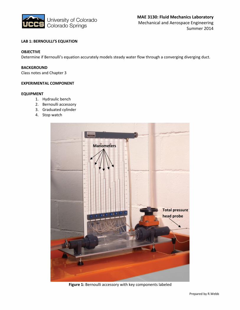
MAE 3130: Fluid Mechanics Laboratory Mechanical and Aerospace Engineering

Summer 2014

Prepared by R.Webb

LAB 1: BERNOULLI’S EQUATION OBJECTIVE Determine if Bernoulli’s equation accurately models steady water flow through a converging diverging duct. BACKGROUND Class notes and Chapter 3 EXPERIMENTAL COMPONENT EQUIPMENT

1. Hydraulic bench 2. Bernoulli accessory 3. Graduated cylinder 4. Stop watch

Figure 1: Bernoulli accessory with key components labeled

Manometers

Total pressure head probe

MAE 3130: Fluid Mechanics Laboratory Mechanical and Aerospace Engineering

Summer 2014

Prepared by R.Webb

PROCEDURE: • Crack the bench flow control valve (black knob located on the front of the hydraulic bench) • Turn on pump (pump power switch on front of the hydraulic bench) • Set the flow rate to 10 ml/s

o Slowly open the flow control valve o Measure the flow rate o Adjust the flow control valve up or down to achieve 10 ml/s o Measure the flow rate o Repeat until flow rate is 10 ml/s o Allow the flow to steady o Measure the flow rate once more to ensure it is 10 ml/s. Adjust if necessary.

• Measure the static pressure head at the different locations along the test section and record. Make sure the total pressure head probe is not in the test section* during this time. *The test section includes the throat, converging and diverging sections. Do NOT remove the total pressure head probe from the system.

• Measure the total pressure head distribution by moving the total pressure head probe along the test section centerline. Measurements should be made at 1 cm intervals. Record measurements.

• Repeat for a minimum of two additional laminar flow rates and three turbulent flow rates.

MAE 3130: Fluid Mechanics Laboratory Mechanical and Aerospace Engineering

Summer 2014

Prepared by R.Webb

COMPUTATIONAL COMPONENT SET-UP:

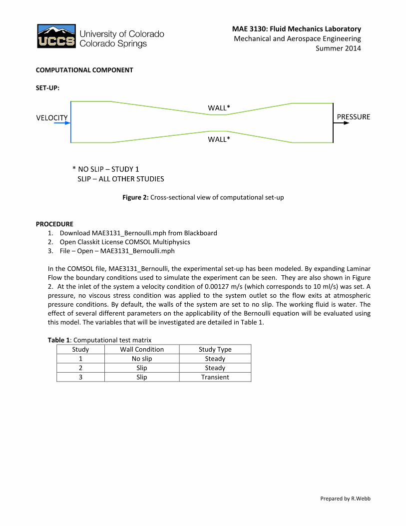
Figure 2: Cross-sectional view of computational set-up PROCEDURE

1. Download MAE3131_Bernoulli.mph from Blackboard 2. Open Classkit License COMSOL Multiphysics 3. File – Open – MAE3131_Bernoulli.mph

In the COMSOL file, MAE3131_Bernoulli, the experimental set-up has been modeled. By expanding Laminar Flow the boundary conditions used to simulate the experiment can be seen. They are also shown in Figure 2. At the inlet of the system a velocity condition of 0.00127 m/s (which corresponds to 10 ml/s) was set. A pressure, no viscous stress condition was applied to the system outlet so the flow exits at atmospheric pressure conditions. By default, the walls of the system are set to no slip. The working fluid is water. The effect of several different parameters on the applicability of the Bernoulli equation will be evaluated using this model. The variables that will be investigated are detailed in Table 1. Table 1: Computational test matrix

Study Wall Condition Study Type 1 No slip Steady 2 Slip Steady 3 Slip Transient

MAE 3130: Fluid Mechanics Laboratory Mechanical and Aerospace Engineering

Summer 2014

Prepared by R.Webb

Evaluation 1 Study 1 assumes a no slip condition at the wall. This study has been evaluated and the results are stored in Solution 1. Replace the no slip wall condition of Study 1 with a slip condition and compare the results of the two different studies. 1. Create a steady state study – see instructions in Appendix 1 2. Expand Laminar Flow

a. Wall 1 contains the no slip wall condition b. To replace the no slip condition with a slip condition, enable Wall 2

3. Mesh – Build All 4. Study 2 – Compute

The velocity along the centerline of the system can be extracted from the solution with a cut line placed along the system axis. The cut lines have already been generated, but the correct solution must be assigned to each line. 5. Follow the instructions for generating a 3D cut line in Appendix 2 for Runs 1 and 2. Plot velocity versus position for the different wall conditions. 6. Under Results – expand VelocityVsPosition-WallCondition 7. Follow the instructions for generating a 1D line graph in Appendix 3 for Runs 1 and 2. 8. Click on camera icon above plot, select include and leave color legend and axes selected, save your

figure to a file.

Generate a velocity contour plot to see a global picture of the flow. This requires creating a cut plane which is essentially a plane that cuts through the flow from top to bottom and side to side.

9. Create cut planes using the instructions in Appendix 2 for Runs 1 and 2. 10. Under Results – expand VelocityContour – No Slip 11. Plot the velocity in this plane using the instructions in Appendix 3 for generating a 2D plot group. 12. Click on camera icon above plot, save your figure to a file 13. Add streamlines to this plot.

a. Right click on VelocityContour – No Slip – Streamline. b. Data set: Cut Plane 1 c. Points: 40 d. Plot e. Zoom in on the diffuser exit and wall

14. Click on camera icon above plot, save your figure to a file 15. Repeat for VelocityContour – Slip 16. Click on camera icon above plot, save your figure to a file

Export the no slip and slip centerline velocity data for comparison with the experimental values.

17. Export the data from Study 1 using the instructions for exporting data in Appendix 4 18. Repeat for Study 2.

Evaluation 1 is complete. Save your file as MAE3131_Bernoulli_Eval1

MAE 3130: Fluid Mechanics Laboratory Mechanical and Aerospace Engineering

Summer 2014

Prepared by R.Webb

Evaluation 2 Study 2 assumes a slip condition at the wall and steady state conditions. Evaluate an unsteady flow and compare the results with those of Study 2. 1. Create a transient study – see instructions in Appendix 1 2. Study 3 – Compute

The velocity along the centerline of the system can be extracted from the data with a cut line. The cut line can be placed along the system axis and the data along that cut line evaluated. The cut lines have already been generated, but the correct solution must be assigned to each line. 3. Follow the instructions for generating a 3D cut line in Appendix 2 for Run 3. Plot velocity versus position as a function of time. 4. Under Results – expand VelocityVsPosition-Time 5. Follow the instructions for generating a 1D line graph (transient) in Appendix 3 for Run 3. 6. Click on camera icon above plot, save your figure to a file.

Evaluation 2 is complete. Save your file as MAE3131_Bernoulli_Eval2

MAE 3130: Fluid Mechanics Laboratory Mechanical and Aerospace Engineering

Summer 2014

Prepared by R.Webb

KEY POINTS Experimental data:

• Using the manometer and flow rate measurements calculate total pressure head along the tube for all flow rates evaluated.

• Plot total pressure head versus position for all flow rates evaluated. Use both the total pressure head that was calculated in the previous step and the values that were measured directly.

o Describe the pressure profiles. o Do the calculated and directly measured values for a given flow rate match everywhere? Why or

why not? o Do the calculated and directly measured values match better for some flow rates than others?

Why or why not? Computational data:

• Plot velocity versus position for the no slip and slip computational cases on the same chart as the experimental data for the 10 ml/s run.

o Describe the velocity profiles. o Do these results match expectations (e.g. Is the maximum velocity where you would expect it)?

Explain. o How are the profiles the same? How are they different? What are the reasons for these

differences? • Plot the velocity contours for the no slip and slip cases.

o Describe the contours. o How are the contours the same? How are they different? What are the reasons for these

differences? o Use the close-ups of the streamlines to strengthen your arguments.

• Plot velocity versus position as a function of time. o Describe the velocity profiles. o How do the profiles change with time?

MAE 3130: Fluid Mechanics Laboratory Mechanical and Aerospace Engineering

Summer 2014

Prepared by R.Webb

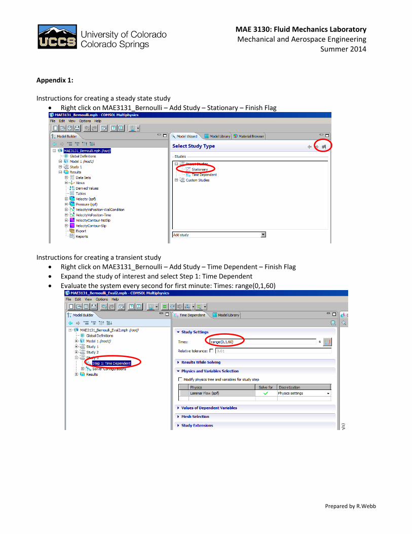
Appendix 1: Instructions for creating a steady state study

• Right click on MAE3131_Bernoulli – Add Study – Stationary – Finish Flag

Instructions for creating a transient study

• Right click on MAE3131_Bernoulli – Add Study – Time Dependent – Finish Flag • Expand the study of interest and select Step 1: Time Dependent • Evaluate the system every second for first minute: Times: range(0,1,60)

MAE 3130: Fluid Mechanics Laboratory Mechanical and Aerospace Engineering

Summer 2014

Prepared by R.Webb

Appendix 2: Instructions for creating a 3D cut line

• Expand Results and then expand Data Sets • Select Cut Line 3D X – Data set: Solution X – Plot (X will change with each study. For example, Study 2

will use Cut Line 3D 2 and Solution 2).

The cut line, shown in red in the graphics pane, runs along the axis of the test piece. The location of this line is dictated by the values input for Point 1 and 2.

MAE 3130: Fluid Mechanics Laboratory Mechanical and Aerospace Engineering

Summer 2014

Prepared by R.Webb

Instructions for creating a cut plane • Expand Results and then expand Data Sets • Select Cut Plane X – Data set: Solution X – Plot

MAE 3130: Fluid Mechanics Laboratory Mechanical and Aerospace Engineering

Summer 2014

Prepared by R.Webb

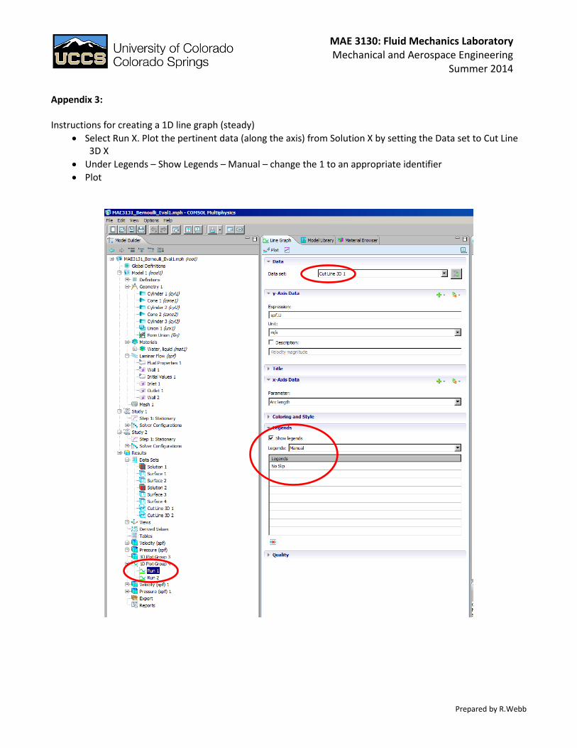
Appendix 3: Instructions for creating a 1D line graph (steady)

• Select Run X. Plot the pertinent data (along the axis) from Solution X by setting the Data set to Cut Line 3D X

• Under Legends – Show Legends – Manual – change the 1 to an appropriate identifier • Plot

MAE 3130: Fluid Mechanics Laboratory Mechanical and Aerospace Engineering

Summer 2014

Prepared by R.Webb

Instructions for creating a 1D line graph (transient) • Select Run X. Plot the pertinent data (along the axis) from Solution X by setting the Data set to Cut Line

3D X • Time selection: Manual • Time indices: range (1,5,60) • Under Legends – Show Legends – Automatic • Plot

Instructions for creating a 2D plot group

• Select Run X. Plot the pertinent data (along the axis) from Solution X by setting the Data set to Cut Plane X

• Plot

MAE 3130: Fluid Mechanics Laboratory Mechanical and Aerospace Engineering

Summer 2014

Prepared by R.Webb

Appendix 4: Instructions for exporting data

1. Right click Export – Data 2. Data set: Cutline 3D X 3. Filename: Descriptive file name 4. Points to evaluate in: Regular grid 5. Number of x points: 100 6. Export