BERNOULLI, RAMANUJAN, TOEPLITZ AND THE TRIANGULAR …difiore/BernoulliBis.pdf · BERNOULLI,...

BERNOULLI, RAMANUJAN, TOEPLITZ AND THE

TRIANGULAR MATRICES

CARMINE DI FIORE, FRANCESCO TUDISCO, AND PAOLO ZELLINI

Abstract. By using one of the definitions of the Bernoulli numbers, we provethat they solve particular odd and even lower triangular Toeplitz (l.t.T.) sys-tems of linear equations. In a paper Ramanujan writes down a sparse lowertriangular system solved by Bernoulli numbers; we observe that such systemis equivalent to a sparse l.t.T. system. The attempt to obtain the sparse l.t.T.Ramanujan system from the l.t.T. odd and even systems, has led us to studyefficient methods for solving generic l.t.T. systems. Such methods are hereexplained in detail in case n, the number of equations, is a power of a genericpositive integer.

1. Introduction

The j-th Bernoulli number, B2j(0), is a rational number defined for any j ∈ N,positive if j is odd and negative if j is even, whose denominator is known, in thesense that it is the product of all prime numbers p such that p−1 divides 2j [11], and,instead, only partial information are known about the numerator [44], [21], [38].Shortly, B2j(0), j ≥ 1, could be defined by the well known Euler formula B2j(0) =

(−1)j+1(2(2j)!/((2π)2j))∑+∞

k=1 1/k2j, involving the Zeta-Riemann function [3], [14].May be the latter formula alone is sufficient to justify the past and present interestin investigating Bernoulli numbers (B.n.). Note that an immediate consequence ofthe Euler formula is the fact that the B2j(0) go to infinite as j diverges.

In literature one finds several identities involving B.n., and also several “explicit”formulas for them, which may appear more explicit than Euler formula since involvefinite (instead of infinite) sums [16], [27], [20], [9], [42], [24], [8], [1]. Some of suchidentities/formulas have been used to define algorithms for the computation of thenumerators of the B.n.. It is however interesting to note that there are efficientalgorithms for such computations which exploit directly the expression of the B.n.in terms of the Zeta-Riemann function [10], [31], [38], [18]. See also [2], [20], [32].As it is noted in [27], the B.n. appear in several fields of mathematics; in particular,the numerators of the B.n. and their factors play an important role in advancednumber theory (see [28], [29], [44], [30], [21]). So, wider and wider lists of the“first” B.n. have been and are compiled, and also lists of the known factors of theirnumerators. The updating of these lists requires the implementation of efficientprimality-test/integer-factorization algorithms on powerful parallel computers. Forinstance, by this way the numerator of B200(0) first has been proved not prime, andthen has been factorized as the product of five prime integers. Two of such factors,respectively of 90 and 115 digits, have been found only very recently [45], [35].

A lower triangular Toeplitz (l.t.T.) matrix A is a square matrix such that aij = 0if i < j, and ai,j = ai+1,j+1, for all i, j. The product of two l.t.T. matrices whateverorder is used generates the same matrix, and such matrix is l.t.T.. If A l.t.T. is non

1991 Mathematics Subject Classification. 11B68, 11Y55, 15A06, 15A09, 15A24, 15B05, 15B99,65F05.

Key words and phrases. Bernoulli numbers; triangular Toeplitz matrices.

1

2 CARMINE DI FIORE, FRANCESCO TUDISCO, AND PAOLO ZELLINI

singular then its inverse is l.t.T., and thus is uniquely defined by its first column.Such remarks simply follow from the fact that the set of all l.t.T. matrices is nothingelse than the set {p(Z)} of all polynomials in the lower-shift matrix Z = (δi,j+1),and the fact that {p(X)} is, for any square matrixX , a commutative matrix algebraclosed under inversion.

Note that, given a n × n l.t.T. matrix A, multiplying A by a vector (M), orsolving a system whose coefficient matrix is A (S), are both operations that canbe performed in at most O(n log n) arithmetic operations, thus in an amount ofoperations significantly smaller than, for example, the n(n + 1)/2 multiplicativeoperations required by the standard algorithm for lower triangular (non Toeplitz)matrices. Such performances are possible by introducing alternative algorithmswhich exploit, first, the strict relationship between the Toeplitz structure and thediscrete Fourier transform – which can be resumed in circulant matrices [13] –,and second, the fast implementation, known as FFT, of the latter. However, for(M) and (S) it is not so clear what is the best possible alternative algorithm. Inparticular, two well known procedures performing the multiplication l.t.T. matrix× vector hold unchanged if the l.t.T. is replaced by a generic (full) Toeplitz matrix;so one guesses that better algorithms may be introduced, ad hoc for the l.t.T. case.Analogously, a widely known exact algorithm able to solve l.t.T. systems (or, moreprecisely, to compute the first column of the inverse of a l.t.T. matrix) in at mostO(n log n) a.o., has essentially a recursive character, which is not so convenient fromthe point of view of the space complexity [33]. In order to avoid such drawback,one could use approximation inverse algorithm [6], [25]. See also [41], [40], [39], [4],[26], [37], [25]. Note that improving the constant c in the complexity cn logn ofl.t.T. solvers is the subject of recent researches, see for example [17].

In this paper we emphasize the connection (may be also noted elsewhere, seef.i. [15]) between Bernoulli numbers and lower triangular Toeplitz matrices. Thisconnection will finally result into new possible algorithms for computing simulta-neously the first n Bernoulli numbers. More precisely, in Section 3 we prove thatthe vector z = (B2j(0)xj/(2j)! )+∞

j=0 , x ∈ R (B0(0) = 1), solves three type I l.t.T.semi-infinite linear systems Ax = f , named even, odd and Ramanujan, respectively.To such systems correspond other three systems, of type II, solved by the vectorZT z = (B2j(0)xj/(2j)! )+∞

j=1 . Type I ad II l.t.T. systems have been obtained asfollows:

- Introducing/considering three particular lower triangular systems solved byBernoulli numbers. The first two, which we may call almost-even and almost-

odd, are introduced by exploiting a well known power series expansion involvingBernoulli polynomials. It is interesting to note that the coefficient matrices of suchsystems are particular submatrices of the l.t. Tartaglia-Pascal matrix. The thirdone, the almost-Ramanujan system, is deduced from the 11 equations, solved bythe absolute values of the first 11 B.n., listed by Ramanujan in the paper [36].

- Noting that the almost-even, almost-odd, and almost-Ramanujan systems arestructured in such a way that their coefficient matrices can be forced to be Toeplitz.This result follows, for the first two systems, from the matrix series representationof the Tartaglia-Pascal matrix in terms of powers of a kind of regularly weightedlower shift matrix, and, for the third one, by a clever remark proved in the 11× 11case, and conjectured in the general case.

- Proving that each of the three l.t.T. systems so obtained – even, odd andRamanujan –, which is solved by z (or ZT z), can be manipulated so to define acorrespondent l.t.T. system whose solution is ZT z (or z).

BERNOULLI, RAMANUJAN, TOEPLITZ AND THE TRIANGULAR MATRICES 3

The lower triangular system written by Ramanujan in [36] has the remarkablepeculiarity to have two null diagonals alternating the nonnull ones. The samepeculiarity is inherited by its (lower triangular) Toeplitz version, obtained in thispaper (see (16), (18), (19)). The attempt to obtain the l.t.T. Ramanujan system,and, more in general, sparse and simple l.t.T. systems solved by Bernoulli numbers,directly from the odd and even l.t.T. systems, has led us to study, using a simplematrix formulation, fast direct (not recursive) solvers of generic l.t.T. systems. Infact, the process of making null two diagonals every one, can be repeated, so tofinally transform the initial l.t.T. into the identity matrix. Each step of such sort ofGaussian elimination procedure – where diagonals, instead of columns, are nullified– is realized by a left multiplication by a suitable l.t.T. matrix whose dimension is infact 2/3 smaller than in the previous step. This leads to a O(n log3 n) exact solverof l.t.T. systems Ax = f where A is n× n with n = 3s, the G3 algorithm, and thento a general exact low complexity Gb procedure, ad hoc for the case n = bs with bgeneric. The algorithm Gb, with b = 2, 3 and b generic, is illustrated in Section 4.Note that the first step of G3 can be skipped when solving the Ramanujan l.t.T.system, as, we may say, it has been already performed explicitly by Ramanujan.The simplicity of the algorithm Gb and, in particular, the clearness of its matrixformulation could suggest its consideration in the wide literature on low complexityl.t.T. solvers [6], [5], [25], [12], [7], [33], [34], [41], [22], [37], [17], [43].

2. Preliminaries on lower triangular Toeplitz (l.t.T.) matrices

Let Z be the following n× n matrix

Z =

01

1·

1 0

.

Z is usually called lower-shift due to the effect that its multiplication by a vectorv = [v0 v1 · · · vn−1]

T ∈ Cn produces: Zv = [0 v0 v1 · · · vn−2]T . Let L be the

subspace of Cn×n of those matrices which commute with Z. It is simple to observethat L is a matrix algebra closed under inversion, that is if A,B ∈ L then AB ∈ Land if A ∈ L is nonsingular then A−1 ∈ L. Let us investigate the structure of thematrices in L. Let A ∈ Cn×n. Then

AZ =

a12 · a1n 0...

......

an2 · ann 0

, ZA =

0 · · · 0a11 · · · a1n

· ·an−11 · · · an−1n

.

Forcing the equality between AZ and ZA we obtain the conditions a12 = a13 =. . . a1n = a2n = . . . an−1,n = 0 and ai,j+1 = ai−1,j , i = 2, . . . , n, j = 1, . . . , n − 1,from which one deduces the structure of A ∈ L: A must be a lower triangularToeplitz (l.t.T.) matrix, i.e. a matrix of the type

(1) A =

a11

a21 a11

a31 a21 a11

· · ·an1 · · a21 a11

.

It follows that dimL = n and that, by a well known general result [23], L can berepresented as the set of all polynomials in Z, i.e. L = {p(Z) : p = polynomials} .


Actually, by investigating the powers of Z one realizes that the matrix A in (1) isexactly the polynomial

∑nk=1 ak1Z

k−1.Note also that, as a consequence of the above arguments, the inverse of a l.t.T.

matrix is still l.t.T., thus it is completely determined as soon as its first column isknown. In Section 4 we will illustrate a low complexity exact algorithm Gb for thesolution of a l.t.T. linear system Ax = f , A ∈ L, A11 = 1, where n = bs with b = 2, 3and b generic. The implementation of Gb requires the availability of a procedureable to perform a matrix-vector product where the matrix is l.t.T. m × m withm = bj (j = 2, . . . , s). More efficient is such procedure, lower is the complexity ofthe algorithm. So, let us briefly discuss the complexity of the computation l.t.T.matrix×vector.

The product of a m × m l.t.T. matrix times a vector can be computed withmuch less than the m(m+ 1)/2 multiplications and (m− 1)m/2 additions requiredby the obvious algorithm. In fact, two alternative known procedures reduce therequired computation to a small number of FFT of order m or bm, i.e., if m = bj ,to no more than cbjb

j arithmetic operations, where cb is a constant. This resultis obtained by using a) two representations of a generic Toeplitz matrix involvingcirculant and (−1)-circulant matrix algebras and b) the fact that the matrices ofsuch algebras are simultaneously diagonalized by the discrete Fourier transform(DFT) or scalings of the DFT [13]. For the sake of completeness, here we brieflyrecall the two representations, by noting however that both do not improve at

all when the Toeplitz matrix is lower triangular. It follows that lower complexityprocedures, for the l.t.T. matrix by vector product computation, could exist andwould be welcome.

Let Π±1 be the m×m matrix Π±1 = ZT ± emeT1 , where Z is the m×m lower-

shift matrix. Given any vector aT = [a1 a2 · · ·am], the circulant and skew circulant

matrices whose first row is aT , are, respectively,

C(a) =

m∑

k=1

akΠk−11 and C−1(a) :=

m∑

k=1

akΠk−1−1

Let T = (ti−j)mi,j=1, tk ∈ C, be a Toeplitz matrix, and let v be any vector of Cm.

The matrix T is the upper left submatrix of a bm× bm circulant matrix C(a), i.e.

(2) T = {C(a)}m, aT = [t0 t−1 · t−m+1 0T(b−2)m+1 tm−1 · t1].

Thus

Tv = {C(a)

[

v0(b−1)m

]

}m,

where the symbol {z}m denotes the m × 1 vector whose entries are the first mcomponents of z. If, for example, m is a power of b (b = 2, 3, . . .), such equalityallows to perform very efficiently the product Tv, by the tool of FFT. The Toeplitzmatrix T can be alternatively represented as the sum of a circulant and a skewcirculant matrix. In fact,

T = C(a) + C−1(a′),(3)

ai =1

2(t−i+1 + tm−i+1), a

′i =

1

2(t−i+1 − tm−i+1), i = 1, . . . ,m

(tm = 0). Again, if m = bj (b = 2, 3, . . .), from this formula one immediatelydeduces a procedure computing Tv in no more than cbjb

j arithmetic operations.


3. Bernoulli numbers and triangular Toeplitz matrices

The following three conditions

B(x + 1) −B(x) = nxn−1,

∫ 1

0

B(x) dx = 0, B(x) polinomio

uniquely define the function B(x). It is a particular degree n monic polynomialcalled n-th Bernoulli polynomial and usually denoted by the symbol Bn(x). It issimple to compute the first Bernoulli polynomials:

B1(x) = x− 1

2, B2(x) = x(x− 1) +

1

6, B3(x) = x(x − 1

2)(x− 1), . . . .

B0(x) is assumed equal to 1.It can be proved that Bernoulli polynomials define the coefficients of the power

series representation of several functions, for instance to our aim it is useful to recallthat the following power series expansion holds:

(4)text

et − 1=

+∞∑

n=0

Bn(x)

n!tn.

Moreover, Bernoulli polynomials satisfy many identities. Among all we recall thefollowing ones, concerning the value of their derivatives and their property of sym-metry with respect to the line x = 1

2 :

B′n(x) = nBn−1(x), Bn(1 − x) = (−1)nBn(x).

It is simple to observe as a consequence of their definition and of the last identitythat all the Bernoulli polynomials with odd degree (except B1(x)) vanish for x = 0.On the contrary, the value that an even degree Bernoulli polynomial attains inthe origin is different from zero and especially important. In particular, recall thefollowing Euler formula

ζ(2j) =|B2j(0)|(2π)2j

2(2j)!, ζ(s) =

+∞∑

k=1

1

ks,

which shows the strict relation between the numbers B2j(0) and the values thatthe Riemann Zeta function ζ(s) attains over all even positive integer numbers 2j[14], [3]. For instance, from such relation and from the fact that ζ(2j) → 1 if j →+∞, one deduces that |B2j(0)| tends to +∞ almost the same way as 2(2j)!/(2π)2j

does. Another important formula involving the valuesB2j(0) is the Euler-Maclaurinformula [14], which is useful in particular for the computation of sums: if f is asmooth enough function over [m,n], m,n ∈ Z, then

n∑

r=m

f(r) =1

2[f(m) + f(n)] +

∫ n

m

f(x) dx(5)

+

k∑

j=1

B2j(0)

(2j)![f (2j−1)(n) − f (2j−1)(m)] + uk+1,

where

uk+1 =1

(2k + 1)!

∫ n

m

f (2k+1)(x)B2k+1(x) dx

= − 1

(2k)!

∫ n

m

f (2k)(x)B2k(x) dx

=1

(2k + 2)!

∫ n

m

f (2k+2)(x)[B2k+2(0) −B2k+2(x)] dx


and Bn is Bn|[0,1) extended periodically over R. Let us recall that the Euler-Maclaurin formula also leads to an important representation of the error of the

trapezoidal rule Ih = h[ 12g(a) +∑n−1

r=1 g(a+ rh) + 12g(b)], h = b−a

n , in the approx-

imation of the definite integral I =∫ b

a g(x) dx. Such representation, holding forfunctions g which are smooth enough in [a, b], is obtained by setting m = 0 andf(t) = g(a+ th) in (5):

Ih = I +

k∑

j=1

h2jB2j(0)

(2j)![g(2j−1)(b) − g(2j−1)(a)] + rk+1,(6)

rk+1 =g(2k+2)(ξ)h2k+2(b− a)B2k+2(0)

(2k + 2)!,

ξ ∈ (a, b). The representation in (6) of the error, in terms of even powers of h,shows the reason why the Romberg extrapolation method for estimating a definiteintegral is efficient, when combined with trapezoidal rule. From (6) it is indeed

clear that Ih/2 := (22Ih/2 − Ih)/(22 − 1) approximates I with an error of order

O(h4), whereas the error made by Ih and Ih/2 is of order O(h2).For these and other applications/theories where the Bernoulli numbers B2j(0)

are involved, see for instance [30], [28], [27], [14], [3].

3.1. Bernoulli numbers solve triangular Toeplitz systems. From (4) it fol-lows that Bernoulli numbers satisfy the following identity

t

et − 1= −1

2t+

+∞∑

k=0

B2k(0)

(2k)!t2k.

Multiplying the latter by et−1, expanding et in terms of powers of t, and setting tozero the coefficients of ti of the right hand side, i = 2, 3, 4, . . ., yields the followingequations:

(7) −1

2j +

[ j−1

2]

∑

k=0

(

j2k

)

B2k(0) = 0, j = 2, 3, 4, . . . .

Now, putting together equations (7) for j even and for j odd, we obtain two lowertriangular linear systems that uniquely define Bernoulli numbers:

(

20

)

(

40

) (

42

)

(

60

) (

62

) (

64

)

(

80

) (

82

) (

84

) (

86

)

· · · · ·

B0(0)B2(0)B4(0)B6(0)

·

=

1234·

,

(

10

)

(

30

) (

32

)

(

50

) (

52

) (

54

)

(

7

0

) (

7

2

) (

7

4

) (

7

6

)

· · · · ·

B0(0)B2(0)B4(0)B6(0)

·

=

13/25/27/2·

.

So, we can for instance easily compute the first Bernoulli numbers:

(8) 1,1

6, − 1

30,

1

42, − 1

30,

5

66, − 691

2730,

7

6, −3617

510.


The coefficients matrices We and Wo of such linear systems turn out to have ananalytic representation. In order to prove this fact, it is enough to observe that We

and Wo are suitable submatrices of the Tartaglia-Pascal matrix X , which can berepresented as a power series. More precisely, set

Y = Z · diag(

i : i = 1, 2, 3, . . .)

, φ = Z · diag(

(2i− 1)2i : i = 1, 2, 3, . . .)

where Z is the semi-infinite lower shift matrix Z = (δi,j+1)+∞i,j=1, and note that for

all i, j, 1 ≤ j ≤ i ≤ n, we have

[

+∞∑

k=0

1

k!Y k]ij =

1

(i− j)![Y i−j ]ij =

1

(i− j)!j · · · (i− 2)(i− 1) =

(

i − 1j − 1

)

,

or, equivalently,

X :=

(

00

)

(

1

0

) (

11

)

(

2

0

) (

21

) (

22

)

(

3

0

) (

31

) (

3

2

) (

33

)

(

4

0

) (

41

) (

4

2

) (

43

) (

44

)

(

5

0

) (

51

) (

5

2

) (

53

) (

5

4

) (

55

)

(

6

0

) (

61

) (

6

2

) (

63

) (

6

4

) (

65

) (

66

)

· · · · · · · ·

=

+∞∑

k=0

1

k!Y k.

Then, simple investigations allows one to observe that We and Wo, which are thel.t. matrices obtained by putting together, respectively, the bold and italic binomialentries of X , can be represented in terms of power series in the matrix φ, i.e.

We = ZTφ ·+∞∑

k=0

1

(2k + 2)!φk, Wo = ψ ·

+∞∑

k=0

1

(2k + 1)!φk ,

where ψ = diag(

2i− 1 : i = 1, 2, 3, . . .)

. We can therefore rewrite the two linearsystems solved by Bernoulli numbers as follows:

(9)

+∞∑

k=0

2

(2k + 2)!φkb = qe, b =

B0(0)B2(0)B4(0)B6(0)

·

, qe =

11/31/51/7·

,

(10)

+∞∑

k=0

1

(2k + 1)!φkb = qo, qo =

11/21/21/2·

.

Now, let us show that systems (9) and (10) are equivalent to two l.t.T. linear sys-tems. Our aim is to replace φ, a matrix whose subdiagonal entries are all different,by a matrix whose subdiagonal entries are all equal.

Set D = diag (d1, d2, d3, . . .), di 6= 0. By investigating the nonzero entries ofthe matrix DφD−1, it is easy to observe that it can be forced to be equal to a


matrix of the form xZ; just choose dk = xk−1d1/(2k − 2)!, k = 1, 2, 3, . . .. So, if

(11) D = diag(

1,x

2!,x2

4!, · , xn−1

(2n− 2)!, ·

)

,

we have the equality DφD−1 = xZ.Now, since DφkD−1 = (DφD−1)k = xkZk, it is easy to show the equivalence of

(9) and (10) with the following l.t.T. linear systems:

(12)

+∞∑

k=0

2xk

(2k + 2)!ZkDb = Dqe,

(13)

+∞∑

k=0

xk

(2k + 1)!ZkDb = Dqo.

Summarizing, let z be the vector Db. Then the vector {b}n whose entries are thefirst n Bernoulli numbers can be obtained by a two-phase procedure:

1. compute the first n components of the solution of the l.t.T. system (12)((13)), i.e. compute {z}n such that

{+∞∑

k=0

2xk

(2k + 2)!Zk }n{z}n = {Dqe}n

(

{+∞∑

k=0

xk

(2k + 1)!Zk }n{z}n = {Dqo}n

)

2. solve the linear system {D}n{b}n = {z}n over the rational field.

The computation in phase 1 can be done by means of the algorithm described inthe next Section 4 at a computational cost of O(n log n) arithmetic operations.It is important to note that such algorithm can be made numerically stable bya suitable choice of the parameter x. For instance, the choice x = (2π)2 wouldensure the sequence {zn} = {xnB2n(0)/(2n)!} to be bounded; indeed in this case|zn| → 2 if n → +∞, due to Euler formula. So, in phase 1, one obtains n machinenumbers which are good approximations in R of the quantities xiB2i(0)/(2i)!, i =0, 1, . . . , n−1. Then, in phase 2, one should find a way to deduce, from the machinenumbers obtained, the rational Bernoulli numbers B2i(0), i = 0, 1, . . . , n− 1.

3.2. The Ramanujan l.t.T. linear system solved by Bernoulli numbers. In[36] Ramanujan writes explicitly 11 sparse equations solved by the absolute valuesof the 11 Bernoulli numbers B2(0), B4(0), . . ., B22(0). They are the first of aninfinite set of sparse equations solved by the absolute values of all the Bernoullinumbers. The Ramanujan equations, written together and directly in terms of theB2i := B2i(0), i = 1, 2, . . . , 11, form the linear system displayed here below:

10 10 0 113 0 0 10 5

2 0 0 10 0 11 0 0 115 0 0 143

4 0 0 10 4 0 0 286

3 0 0 10 0 204

5 0 0 221 0 0 117 0 0 1938

7 0 0 32307 0 0 1

0 112 0 0 7106

5 0 0 35534 0 0 1

· · · · · · · · · · · ·

B2

B4

B6

B8

B10

B12

B14

B16

B18

B20

B22

·

=

16

− 130142145

− 11324

4551

120− 1

3063

6651

231− 1

552·

.


For example, by using the last but three of Ramanujan equations, from the Bernoullinumbers B2(0), . . . , B16(0) listed in (8), the following further Bernoulli numbers canbe easily obtained:

B18(0) =43867

798, B20(0) = −174611

330, B22(0) =

854513

138.

Let R be the semi-infinite coefficient matrix of the above Ramanujan system. Byrecalling the definition of the semi-infinite lower shift matrix Z and of the semi-infinite vector b = [B0(0)B2(0)B4(0) · ]T , the Ramanujan system can be shortlyindicated as

(14) R(ZT b) = ZT f ,

where ZT f , f = [f0 f1 f2 f3 · ]T , denotes the right hand side vector, i.e. f1 = 1/6,f2 = −1/30, f3 = 1/42, f4 = 1/45, . . ..

Apparently the non-zero entries of R are not related with each other, and itseems so also for the entries of f . That is, it seems to be not possible to guess,just by looking at the above 11 equations, the twelfth equation of the Ramanujansystem. We can only guess that the non-zero entries of R are in the same positionsas the non-zero entries of a l.t.T. matrix R of the form

∑+∞k=0 wkZ

3k, and, maybe,it is possible to guess the sign of the entries of f .

Actually, by a clever remark we noted that the following identity must hold

(15) RΛ−1 = Λ−1R, Λ = ZTDZ = diag( xi

(2i)!: i = 1, 2, 3, . . .

)

,

where D is defined in (11) and R is the following l.t.T. matrix:

R =

+∞∑

k=0

2x3k

(6k + 2)!(2k + 1)Z3k

=

10 10 0 1

2x3

8!3 0 0 1

0 2x3

8!3 0 0 1

0 0 2x3

8!3 0 0 12x6

14!5 0 0 2x3

8!3 0 0 1

0 2x6

14!5 0 0 2x3

8!3 0 0 1

0 0 2x6

14!5 0 0 2x3

8!3 0 0 12x9

20!7 0 0 2x6

14!5 0 0 2x3

8!3 0 0 1

0 2x9

20!7 0 0 2x6

14!5 0 0 2x3

8!3 0 0 1· · · · · · · · · · · ·

.

In fact, the 11× 11 upper left submatrix of RΛ−1 coincides with the 11× 11 upperleft submatrix of Λ−1R.

Assuming that the conjecture (15) is true, we have the equalities R(ZT b) =

RΛ−1(ΛZT b) = Λ−1R(ZTDb), and thus, by (14),

(16) R(ZTDb) = ZTDf .

Hence, the vector ZTDb solves a l.t.T. system which, differently from the l.t.T.systems (12), (13), is sparse, since in its coefficient matrix two null diagonals alter-nate the nonnull ones. Such Ramanujan l.t.T. system will be defined more preciselyin the following (see (18), (19)).


3.3. A unifying theorem with 6 l.t.T. linear systems solved by Bernoullinumbers. Now we collect in a Theorem three l.t.T. linear systems solved by thevector Dxb, say of type I, and the corresponding l.t.T. linear systems solved by thevector ZTDxb, say of type II (Dx is the matrix D in (11)). In fact, till now, wehave only found two systems of type I, the even and odd systems (12) and (13),and, partially, one system of type II, the Ramanujan l.t.T. system (16) (note thatfor the latter system only the coefficient matrix has been written explicitly).

In the following, first we state a Proposition which allows one to state a systemof type II from a system of type I, and viceversa. Then we state the Theorem,with the six l.t.T. linear systems solved by Bernoulli numbers, and we prove it byapplying the Proposition to the even, odd, and Ramanujan l.t.T. systems found tillnow, and, in the same time, by completing the definition of the Ramanujan l.t.T.system.

Proposition 3.1 Let Zn−1 and Zn be the upper-left (n− 1)× (n− 1) and n× nsubmatrices of the semi-infinite lower-shift matrix Z, respectively. Set β = B0(0).Assume that, for some αj and fj (or wj), the following equality holds:

n−1∑

j=0

αjZjn{Dxb}n =

ηx

2!f1

x2

4!f2

·xn−1

(2(n−1))!fn−1

+ β

µ

α1

α2

·αn−1

(

=

w0x

2!w1

x2

4!w2

·xn−1

(2(n−1))!wn−1

)

,

where η and µ are arbitrary parameters. Then we have

n−2∑

j=0

αjZjn−1{Z

TDxb}n−1 =

x

2!f1

x2

4!f2

·xn−1

(2(n−1))!fn−1

(

=

x

2!w1

x2

4!w2

·xn−1

(2(n−1))!wn−1

−β

α1

α2

·αn−1

)

.

Also the converse is true provided that α0β = η + βµ (or α0β = w0).

Proof. Exploit the equality Zn =

[

0 0T

e1 Zn−1

]

. The details are left to the reader.

�

Theorem 3.2 Set Z = (δi,j+1)+∞i,j=1, a = (ai)

+∞i=0 , and L(a) =

∑+∞i=0 ai Z

i. Let

d(w) be the diagonal matrix with wi as diagonal entries. Set

b = [B0(0) B2(0) B4(0) · ]T , Dx = diag( xi

(2i)!: i = 0, 1, 2, . . .

)

, x ∈ R,

where B2i(0), i = 0, 1, 2, . . ., are the Bernoulli numbers. Then the vectors Dxb and

ZTDxb solve the following l.t.T. linear systems

(17) L(a) (Dxb) = Dxq,

(18) L(a) (ZTDxb) = d(w)ZTDxq,

where the vectors a = (ai)+∞i=0 , q = (qi)

+∞i=0 , and w = (wi)

+∞i=1 , can assume respec-

tively the values:

(19)

aRi = δi=0 mod 3

2xi

(2i+ 2)!( 23 i+ 1)

, i = 0, 1, 2, 3, . . .

qRi =

1

(2i+ 1)(i+ 1)(1 − δi=2 mod 3

3

2), i = 0, 1, 2, 3, . . .

wRi = 1 − δi=0 mod 3

123 i+ 1

, i = 1, 2, 3, . . . ,


(20)ae

i =2xi

(2i+ 2)!, i = 0, 1, 2, 3, . . . , qe

i =1

2i+ 1, i = 0, 1, 2, 3, . . .

wei =

i

i+ 1, i = 1, 2, 3, . . . ,

(21)ao

i =xi

(2i+ 1)!, i = 0, 1, 2, 3, . . . , qo

0 = 1, qoi =

1

2, i = 1, 2, 3, . . .

woi =

2i− 1

2i+ 1, i = 1, 2, 3, . . . .

Proof. From the Ramanujan semi-infinite l.t.T. linear system (16), we obtain thefollowing finite linear system

(22)

∑n−2j=0 αjZ

jn−1{ZTDxb}n−1 =

x2!f1x2

4! f2·

xn−1

(2(n−1))!fn−1

,

αj = δj=0 mod 32xj

(2j+2)!( 23j+1)

,

f1 = 16 , f2 = − 1

30 , f3 = 142 , f4 = 1

45 , f5 = − 1132 , f6 = 4

455 ,f7 = 1

120 , f8 =,− 1306 f9 = 3

665 , f10 = 1231 , f11 = − 1

552 , . . . .

Then, by Proposition 3.1, if η +B0(0)µ = α0B0(0), we have that

n−1∑

j=0

αjZjn{Dxb}n =

ηx2!f1x2

4! f2·

xn−1

(2(n−1))!fn−1

+B0(0)

µα1

α2

·αn−1

,

or, more precisely, that

(I +2

8!3x3Z3 +

2

14!5x6Z6 +

2

20!7x9Z9 + . . .)

[

(

xi

(2i)!B2i(0))11

i=0

·

]

=

1x2!

16

x2

4! (− 130 )

x3

6!142 + 2x3

8!3x4

8!145

x5

10! (− 1132 )

x6

12!4

455 + 2x6

14!5x7

14!1

120x8

16! (− 1306 )

x9

18!3

665 + 2x9

20!7x10

20!1

231x11

22! (− 1552 )

·

=

10!(

11·1 )

x2!(

13·2 )

x2

4! (1

5·3 − 15·2 )

x3

6! (1

7·4 )x4

8! (1

9·5 )x5

10! (1

11·6 − 111·4 )

x6

12! (1

13·7 )x7

14! (1

15·8 )x8

16! (1

17·9 − 117·6 )

x9

18! (1

19·10 )x10

20! (1

21·11 )x11

22! (1

23·12 − 123·8 )

·

.

The latter equality is a clever remark that allows us to guess that Dxb must solvethe following Ramanujan l.t.T. system of type I:

(23)

+∞∑

i=0

αiZiDxb = Dxq

R, αi = aRi ,


with aRi and qR

i , i = 0, 1, 2, 3, . . ., defined as in (19). Note that from the explicitexpression of qR just obtained, it follows an explicit expression for all the entriesfi of the original Ramanujan system (14), i.e. also for the fi with i ≥ 12

fi =1

(2i+ 1)(i+ 1)(1 − δi=2 mod 3

3

2− δi=0 mod 3

123 i+ 1

), i = 1, 2, 3, . . . .

Note also that (22) can be rewritten as

n−2∑

j=0

αjZjn−1{ZTDxb}n−1 = diag (wi, i = 1, 2, . . . , n− 1){ZTDxq

R}n−1

for suitable wi. Such wi are easily obtained by imposing the equality

(1 − δi=2 mod 3

3

2− δi=0 mod 3

123 i+ 1

) = wi(1 − δi=2 mod 3

3

2),

which leads to the formula:

wi = 1 −δi=0 mod 3

123i+1

1 − δi=2 mod 332

= 1 − δi=0 mod 3

123 i+ 1

.

So, the l.t.T. type I and type II systems (17), (18) and (19) hold.Now let us consider the finite versions of the even and odd systems (12) and (13),

n−1∑

j=0

2xj

(2j + 2)!Zj

n{Dxb}n = {Dxqe}n,

n−1∑

j=0

xj

(2j + 1)!Zj

n{Dxb}n = {Dxqo}n,

and apply to them Proposition 3.1:

n−2∑

j=0

2xj

(2j + 2)!Zj

n−1{ZTDxb}n−1

=

x2!

13

x2

4!15·

xn−1

(2(n−1))!1

2n−1

−B0(0)

2x4!

2x2

6!·

2xn−1

(2n)!

=

x 24!

x2 46!

x3 68!·

xn−1 2(n−1)(2n)!

,

n−2∑

j=0

xj

(2j + 1)!Zj

n−1{ZTDxb}n−1

=

x2!

12

x2

4!12·

xn−1

(2(n−1))!12

−B0(0)

x3!x2

5!·

xn−1

(2n−1)!

=

x 13!2

x2 35!2

x3 57!2·

xn−1 2n−3(2n−1)!2

.

From the above identities it follows that

n−2∑

j=0

2xj

(2j + 2)!Zj

n−1{ZTDxb}n−1 = 2

x2!

14·3

x2

4!2

6·5x3

6!3

8·7·

xn−1

(2(n−1))!n−1

2n(2n−1)

= diag (i

i+ 1, i = 1 . . . n− 1){ZTDxq

e}n−1,


n−2∑

j=0

xj

(2j + 1)!Zj

n−1{ZTDxb}n−1 =

x2!

12·3

x2

4!3

2·5x3

6!5

2·7·

xn−1

(2(n−1))!2n−3

2(2n−1)

= diag (2i− 1

2i+ 1, i = 1 . . . n− 1){ZTDxq

o}n−1.

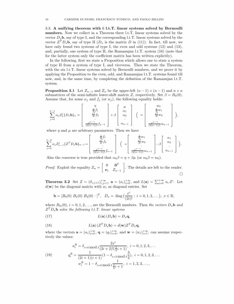
So, also even and odd type II linear systems (18), (20) and (21) hold. �

Remark. From (17) of Theorem 3.2 we have the following formula for B2n(0):

(24) B2n(0) =(2n)!

xn(J{L(a)}−1

n+1e1)T {Dq}n+1,

where J = (δi,n+2−j)n+1i,j=1 is the anti-identity. So, the computation of {L(a)}−1

n+1e1

(for example via the Gb procedure in subsection 4.5) yields B2n(0).

Now it is clear that the first n Bernoulli numbers B2i(0), unless the factorsxi/(2i)!, solve l.t.T. systems Ax = f , where A is the n× n upper left submatrix ofthe semi-infinite matrix L(a) in (17) (or (18)). Throughout the next Section 4 wedescribe an algorithm that can be used to compute the products (xi/(2i)!)B2i(0).

4. An algorithm for the solution of l.t.T. linear systems

In this section we first present an algorithm G2 of complexity O(n log2 n) forthe computation of x such that Ax = f , where A is a n × n l.t.T. matrix, with[A]11 = 1 (which of course is not restrictive) and n = 2s for some s ∈ N. Then, insubsection 4.5, we illustrate the algorithm Gb, which solves the more general casen = bs, where b is a generic positive integer.

4.1. Preliminary Lemmas. Given a vector v = [v0 v1 v2 · · · ]T , vi ∈ C (brieflyv ∈ CN), let L(v) be the semi-infinite l.t.T. matrix whose first column is v, i.e.

L(v) =

+∞∑

k=0

vkZk, Z =

01 0

1 0· ·

.

Lemma 4.1 Let a,b, c ∈ CN. Then L(a)L(b) = L(c) if and only if L(a)b = c.

Proof. If L(a)L(b) = L(c), then the first column of L(a)L(b) must be equal to thefirst column of L(c), and these are the vectorsL(a)b and c, respectively. Conversely,assume that L(a)b = c and consider the matrix L(a)L(b). It is l.t.T., being aproduct of l.t.T matrices, and, by hypothesis, its first column, L(a)b, coincideswith the vector c, which in turn is the first column of the l.t.T. matrix L(c). Thethesis follows from the fact that l.t.T. matrices are uniquely defined by their firstcolumns. �

Given a vector v = [v0 v1 v2 · · · ]T ∈ CN, let E be the semi-infinite matrix withentries 0 or 1, which maps v into the vector Ev = [v0 0 v1 0 v2 0 · · · ]T :

E =

100 10 00 0 1· · · ·

.


In other words, the application of E to v has the effect of inserting a zero betweentwo consecutive components of v. It is easy to observe that

E2 =

10000 10 00 00 00 0 1· · · ·

, Ek =

100 10 00 0 1· · · ·

, 0 = 02k−1,

that is the application of Ek to v has the effect of inserting 2k − 1 zeros betweentwo consecutive components of v.

Lemma 4.2 Let u,v ∈ CN with u0 = v0 = 1. Then L(Eu)Ev = EL(u)v, and,more in general, for each k ∈ N, L(Eku)Ekv = EkL(u)v.

Proof. By inspecting the vectors L(Eu)Ev and EL(u)v one observes that they areequal. By multiplying E on the left of the identity L(Eu)Ev = EL(u)v and usingthe same identity also for the vectors Eu and Ev, in place of u and v respectively,one observes that it also holds L(E2u)E2v = E2L(u)v. And so on. �

4.2. The algorithm G2. Let A be a n×n l.t.T. matrix, with n = 2s and [A]11 = 1.Assume we want to solve the system Ax = f , f ∈ Cn. The algorithm presentedbelow exploits the fact that A−1 is still a n× n l.t.T. matrix.

1. Compute the first column of the l.t.T. matrix A−1 by solving the particularlinear system Ax = e1 via the G2 procedure of complexity O(n log2 n)described in the next subsection 4.3, based upon Lemmas 4.1, 4.2 and theirrepeated application.

2. Use one of the representations (2), (3) (with b = 2) for the l.t.T. matrix A−1

to compute the matrix-vector product A−1f with no more than O(n log2 n)arithmetic operations.

4.3. The computation of the first column of the inverse of a n × n l.t.T.matrix (n = 2s). The G2 procedure for the computation of x such that Ax = e1

consists of two parts. In the first one, certain particular l.t.T. matrices, with theproperty that their successive left multiplication by the matrix A transforms Ainto the the identity matrix, are introduced and computed. In the second partsuch matrices are successively left multiplied by the vector e1. As it will be clearthroughout what follows, the method is nothing more than a kind of Gaussianelimination, where diagonals are nullified instead of columns. The overall costO(n log2 n) comes from the fact that at each step of the first part a half of theremaining non null diagonals are nullified, and from the fact that in the secondpart the computations can be simplified by exploiting the fact that e1 has only onenonzero component.

The G2 procedure is shown in the particular case n = 8. When suitable it isbriefly discussed what changes in the case n = 2s, s ∈ N; nevertheless such casecan be easily deduced from the considered one, or by setting b = 2 in the generalGb procedure, reported in subsection 4.5.

First of all observe that the 8 × 8 matrix A can be thought as the upper-leftsubmatrix of a semi-infinite l.t.T. matrix L(a), whose first column is [1 a1 a2 ·a7 a8 · ]T . The matrix A is transformed into the identity by three steps:


Step 1. Look for a such that

L(a)a =

1a1 1a2 a1 1a3 a2 a1 1a4 a3 a2 a1 1a5 a4 a3 a2 a1 1a6 a5 a4 a3 a2 a1 1a7 a6 a5 a4 a3 a2 a1 1· · · · · · · · ·

1a1

a2

a3

a4

a5

a6

a7

·

=

10

a(1)1

0

a(1)2

0

a(1)3

0

·

= Ea(1)

for some a(1)i ∈ C, and compute such a

(1)i . The computation of a

(1)i requires, once

a is known, one matrix-vector product where the matrix is l.t.T. 8 × 8 (2s × 2s),or, more precisely, two matrix-vector products where the matrices are l.t.T. 4 × 4(2s−1 × 2s−1). We will see that a is available with no computations.

Note that, due to Lemma 4.1, we have L(a)L(a) = L(Ea(1)), that is the l.t.T.matrix L(a) is transformed into a l.t.T. matrix which alternates a null diagonal toeach nonnull diagonal.

Step 2. Look for a(1) such that

L(Ea(1))Ea

(1)

=

10 1

a(1)1 0 1

0 a(1)1 0 1

a(1)2 0 a

(1)1 0 1

0 a(1)2 0 a

(1)1 0 1

a(1)3 0 a

(1)2 0 a

(1)1 0 1

0 a(1)3 0 a

(1)2 0 a

(1)1 0 1

· · · · · · · · ·

10

a(1)1

0

a(1)2

0

a(1)3

0·

=

100

0

a(2)1

00

0·

= E2a

(2)


(2)i . Note that, due to Lemma 4.2, if

L(a(1))a(1) = Ea(2) then L(Ea(1))Ea(1) = E2a(2). So, the computation of a(2)i

requires, once a(1) is known, one matrix-vector product where the matrix is l.t.T.4×4 (2s−1×2s−1), or, more precisely, two matrix-vector products where the matri-ces are l.t.T. 2×2 (2s−2×2s−2). We will see that a(1) such that L(a(1))a(1) = Ea(2)

is available with no computations.Also note that, due to Lemma 4.1, we have L(Ea(1))L(Ea(1)) = L(E2a(2)), that

is the l.t.T. matrix L(a) is transformed into a l.t.T. matrix which alternates threenull diagonals to each nonnull diagonal.

Step 3. Look for a(2) such that

L(E2a

(2))E2a

(2)

=

10 10 0 10 0 0 1

a(2)1 0 0 0 1

0 a(2)1 0 0 0 1

0 0 a(2)1 0 0 0 1

0 0 0 a(2)1 0 0 0 1

· · · · · · · · ·

1000

a(2)1

000·

=

10000

000·

= E3a

(3)



(3)i . Note that, due to Lemma 4.2, if

L(a(2))a(2) = Ea(3) then L(E2a(2))E2a(2) = E3a(3). So, the computation of a(3)i

requires, once a(2) is known, one matrix-vector product where the matrix is l.t.T.2 × 2 (2s−2 × 2s−2), or, more precisely, two matrix-vector products where the ma-trices are l.t.T. 1× 1 (2s−3 × 2s−3). That is, no operation in our case n = 8, where

no entry a(3)i , i ≥ 1, is needed. We will see that a(2) such that L(a(2))a(2) = Ea(3)

is available with no computations.Also note that, due to Lemma 4.1, we have L(E2a(2))L(E2a(2)) = L(E3a(3)),

that is the l.t.T. matrix L(a) is transformed into a l.t.T. matrix which alternatesseven null diagonals to each nonnull diagonal.

If n = 2s > 8, then proceed this way, until the Step s = log2 n. If otherwisen = 23 = 8, then stop, since the first part of the G2 procedure is complete.

Summarizing, we have proved that

(25) L(E2a(2))L(Ea(1))L(a)L(a) = L(E3a(3))

where the upper left 8×8 submatrices of L(a) and of L(E3a(3)) are the initial l.t.T.matrix A and the identity matrix, respectively:

L(a) =

1a1 1· · ·a7 · a1 1a8 a7 · a1 1· · · · · ·

, L(E3a(3)) =

10 1· · ·0 · 0 1

a(3)1 0 · 0 1· · · · · ·

.

The operations we did so far are: one product l.t.T. 8× 8 · vector plus one productl.t.T. 4 × 4 · vector (if A were n × n with n = 2s the operations required wouldhave been: one product l.t.T. 2s × 2s · vector plus . . . plus one product l.t.T. 4× 4· vector).

Now let us move to our main purpose, compute the first column of A−1, and thuslet us show the second part of the G2 procedure. Consider the following semi-infinitelinear system:

(26) L(a)z = E2v

where v is a generic semi-infinite vector in CN (if A is n× n with n = 2s, then thematrix E in (26) must be raised to the power s − 1 rather than 2). Such systemcan be rewritten as follows

A 0 O

a8 · · · a1 1 0T

· · ·

{z}8

z8·

=

v0000v1000v2·

that is, pointing out the upper part of the system, which consists of only 8 equa-tions. Before proceeding further, let us note that {z}8 is such that A{z}8 =[v0 0 0 0 v1 0 0 0]T , v0, v1 ∈ C. Therefore the choices v0 = 1 and v1 = 0, wouldmake {z}8 equal to the vector we are looking for, A−1e1.


By using the identity (25) and Lemma 4.2 one observes that the system L(a)z =E2v is equivalent to the following one[

I8 O...

. . .

] [

{z}8

...

]

= L(E3a(3))z = L(a)L(Ea(1))L(E2a(2))E2v

= L(a)L(Ea(1))E2L(a(2))v = L(a)EL(a(1))EL(a(2))v.

The matrices involved in the vector L(a)EL(a(1))EL(a(2))v on the right hand sideare lower triangular. Moreover, the upper left square submatrices of E of dimensions8 × 8, 4 × 4 have the second half of their columns null, in fact

{E}8 =

1 0 0 0 0 0 0 00 0 0 0 0 0 0 00 1 0 0 0 0 0 00 0 0 0 0 0 0 00 0 1 0 0 0 0 00 0 0 0 0 0 0 00 0 0 1 0 0 0 00 0 0 0 0 0 0 0

, {E}4 =

1 0 0 00 0 0 00 1 0 00 0 0 0

.

These two observations let us obtain an effective representation of {z}8:

{z}8 = {L(a)}8{E}8{L(a(1))}8{E}8{L(a(2))}8{v}8(27)

= {L(a)}8{E}8,4{L(a(1))}4{E}4,2{L(a(2))}2{v}2.

By using such formula, when v0 = 1, v1 = 0, the vector {z}8 can be computed byperforming the operations: one product l.t.T. 4× 4 · vector plus one product l.t.T.8 × 8 · vector (if A is n× n with n = 2s the operations required would have been:one product l.t.T. 4 × 4 · vector plus . . . plus one product l.t.T. 2s × 2s · vector),that is, as many operations as in the first part of the G2 procedure.

Theorem 4.3 If cj2j is an upper bound for the cost of the product l.t.T. 2j × 2j

· vector, then the overall cost of the G2 procedure for the computation of A−1e1,where A is l.t.T. n × n with n = 2s and A11 = 1, is bounded by c

∑sj=2 j2

j =

O(s2s) = O(n log2 n).

We still have to prove that a vector a such that L(a)a = Ea(1) is indeed availablewith no computations. To this aim it is sufficient to observe that

(28) L(a)(

e1 +

+∞∑

i=1

(−1)iaiei+1

)

= e1 +

+∞∑

i=1

δi=0 mod 2

(

2ai +

i−1∑

j=1

(−1)jajai−j

)

ei+1.

This can be verified by a direct calculation.

4.4. Observations on the algorithm’s core. Given the vector a ∈ CN, theproblem of the computation of a ∈ C

N such that L(a)a = Ea(1), for some a(1) ∈ CN

can also be seen as a polynomial arithmetic problem. In fact, due to Lemma 4.1,the identity L(a)a = Ea(1) is equivalent to the equality L(a)L(a) = L(Ea(1)), i.e.

(

+∞∑

k=0

akZk )(

+∞∑

k=0

akZk ) =

+∞∑

k=0

a(1)k Z2k.

Therefore the polynomial arithmetic problem can be stated as follows:

given a(z) =∑+∞

k=0 akzk, find a polynomial a(z) =

∑+∞k=0 akz

k such that

a(z)a(z) = a(1)0 + a

(1)1 z2 + a

(1)2 z4 + . . . =: a(1)(z)

for some coefficients a(1)i .


Such problem is a particular case of the more general problem: transform a full

polynomial a(z) into a sparse polynomial a(1)(z) =∑+∞

k=0 a(1)k zrk, for a fixed r ∈ N.

It is possible to describe explicitly a polynomial a(z) that realizes such transforma-tion, in fact the following result holds

Proposition 4.4 Given a(z) =∑+∞

k=0 akzk, set a(z) = a(zt)a(zt2) · · · a(ztr−1)

where t is a r-th principal root of the unity (t ∈ C, tr = 1, ti 6= 1 for 0 < i < r).Then

(29) a(z)a(z) = a(1)0 + a

(1)1 zr + a

(1)2 z2r + . . . =: a(1)(z)

for some a(1)i . Moreover, if the coefficients of a are real, then the coefficients of a

are real.

Let us consider two corollaries of Proposition 4.4. For r = 2 we have a(z) =

a(−z), that is we regain the result (28). It is clear that a(−z)a(z) = a(1)0 +a

(1)1 z2 +

a(1)2 z4 + . . . (compare with the Graeffe root-squaring method [19]). In this case the

coefficients of a are available with no computations, we only need to compute the

new coefficients a(1)i .

For r = 3 we have a(z) = a(zt)a(zt2), t = ei2π3 . By Proposition 4.4 the following

equalities a(z)a(zt)a(zt2) = a(1)0 + a

(1)1 z3 + a

(1)2 z6 + . . . and

(30) L(a)L(a) = L(Ea(1)), E =

1000 10 00 00 0 1· · · ·

,

hold for some vector a(1), and the coefficients of a(z) = a(zt)a(zt2) are real, pro-vided that the coefficients of a are. This time, the coefficients of a are not eas-ily readable from the coefficients of a. In order to calculate them, observe thatthe polynomial equality a(z) = a(zt)a(zt2) is equivalent to the matrix identityL(a) = L(p)L(q), where p and q are the vectors of the coefficients of the polyno-mials in z a(zt) and a(zt2), and therefore we get the following formula

(31) a = L(p)q, pi = aiti, qi = ait

2i,

which, taking into account that t = ei2π3 , becomes

(32) a = L(p)p + L(q)q,

pi =

{

ai i = 3j− 1

2ai i 6= 3j, qi =

0 i = 3j

−√

3ai/2 i = 3j + 1√3ai/2 i = 3j + 2

, j = 0, 1, 2, . . . .

Remark. There are infinite possible choices of a for which L(a)a = Ea(1) for somevector a(1). Looking for the simplest among them, i.e. for the simplest vector asuch that (L(a)a)i = 0, i = 2, 3, 5, 6, 8, 9, . . ., we have guessed the following optimalchoice for the ai:(33)

aopti = −

b i−1

2c

∑

r=0

arai−r + δi=0 mod 2a2i2

+ 3

{

∑0s≥ 3−i

6

a i−3

2+3sa i+3

2−3s i odd

∑0s≥ 6−i

6

a i−6

2+3sa i+6

2−3s i even

.


After that, when we have known about the result in Proposition 4.4, we checked ifour optimal aopt

i were equal to the ai obtained by setting r = 3 in the result, i.e.to the ai defined by (31)-(32). As the reader can verify, the answer to our checkwas yes. May be the statement of Proposition 4.4 could be completed with theassertion that the polynomial a(z) proposed as solution of problem (29) is optimal.But is such assertion true in general?

So, a vector a satisfying (30) is computable by one l.t.T. matrix-vector product,and therefore (choose b = 3 in (3),(2) of Section 2) the first 3j entries of such vectorcan be obtained with O(j3j) arithmetic operations. This remark allows to statethat O(s3s) arithmetic operations are sufficient to implement the algorithm G3 forthe computation of A−1f , where A is l.t.T. 3s × 3s (set b = 3 in the next section).Note that, in the G3 algorithm, the l.t.T. matrix A is transformed into the identityby s steps, each consisting in nullifying 2/3 of the remaining non null diagonals. Ofcourse it is convenient to use G3 instead of G2 when solving the Ramanujan l.t.T.systems (17), (18), (19), where the coefficient matrix has two null diagonals whichalternate the non null ones.

4.5. The case n = bs, b generic. Let A be a n × n l.t.T. matrix with A11 = 1and n = bs, where b is a fixed integer greater than 1. We know that if the firstcolumn of the l.t.T. A−1 is known then any system Az = f , f ∈ Cn, can be solvedin O(sbs) arithmetic operations (see Section 2). In this section it is described theGb procedure for the computation of A−1e1.

The Gb procedure is structured in two parts and is very similar to the G2 proce-dure, described in detail in subsection 4.3. The main difference is in the fact that ateach of the s steps of the first part, where A is transformed in the identity matrix,(b − 1)/b (instead of 1/2) of the remaining non null diagonals are nullified. Suchoperation is done by applying Lemma 4.1 and an extension of Lemma 4.2, which isnow stated (its proof is left to the reader).

Let E be the matrix with entries equal to zero or one which, applied to u ∈ CN,has the effect of inserting b − 1 zeros between two consecutive components of u.Thus

E =

1 0 0 · ·0 0 0 · ·0 1 0 · ·0 0 0 · ·0 0 1 0 ·· · · · ·

, 0 = 0b−1, Ek =

1 0 0 · ·0 0 0 · ·0 1 0 · ·0 0 0 · ·0 0 1 0 ·· · · · ·

, 0 = 0bk−1,

u =

1u1

u2

·

, Eu=

10u1

0u2

·

, L(Eu)=

10 Iu1 0T 10 u1I 0 Iu2 0T u1 0T 1· · · · · ·

, 0 = 0b−1.

Lemma 4.5 If u,v ∈ CN and u0 = v0 = 1, then L(Eu)Ev = EL(u)v. Moreover,L(Eku)Ekv = EkL(u)v, ∀ k ∈ N.

The given n×n matrix A can be thought as the upper-left submatrix of a semi-infinite l.t.T. matrix L(a), whose first column is [1 a1 a2 · abs−1 abs · ]T . The twoparts of the Gb procedure are described here below.


Part I. Set a(0) := a, and find a(0), a(1) such that

L(a(0))a(0) = Ea(1) =

10

a(1)1

·

, 0 = 0b−1

(

thus L(a(0))L(a(0)) = L(Ea(1)))

.

Then, for k = 2, . . . , s find a(k−1), a(k) such that

L(a(k−1))a(k−1) = Ea(k) =

10

a(k)1

·

, 0 = 0b−1

(

thus L(Ek−1a(k−1))Ek−1a(k−1) = Eka(k) =

10

a(k)1

·

, 0 = 0bk−1,

and L(Ek−1a(k−1))L(Ek−1a(k−1)) = L(Eka(k)))

.

After the above s steps, we obtain the following identity

(34) L(Es−1a(s−1))L(Es−2a(s−2)) · · · L(Ea(1))L(a(0))L(a(0)) = L(Esa(s))

where the upper left bs×bs submatrices of L(a(0)) and of L(Esa(s)) are, respectively,the initial l.t.T. matrix A and the identity matrix,

L(a(0)) =

A 0 O

abs · · · a1 1 0T

· · · · ·

, L(Esa(s)) =

Ibs 0 O

a(s)1 eT

1 1 0T

· · · · ·

.

Part II. By (34), any system of type L(a(0))z = Es−1v, v ∈ CN, is equivalent tothe following linear system

L(Esa(s))z = L(a(0))L(Ea(1)) · · · L(Es−2a(s−2))L(Es−1a(s−1))Es−1v

= L(a(0))EL(a(1))E · · · EL(a(s−2))EL(a(s−1))v.

Thus any vector{

z}

n, n = bs, such that

A{z}n = {L(a)}n{z}n =

v00v10·

vb−1

0

, 0 = 0bs−1−1

(for example, the vector A−1e1 we are looking for), can be represented as follows

{z}n = {L(a(0))}n{E}n{L(a(1))}n{E}n

· · · {E}n{L(a(s−2))}n{E}n{L(a(s−1))}n{v}n

= {L(a(0))}n{E}n,nb{L(a(1))}n

b{E}n

b, n

b2(35)

· · · {E}b3,b2{L(a(s−2))}b2{E}b2,b{L(a(s−1))}b{v}b,

where {M}j,k denotes the j × k upper left submatrix of M . The latter formulaallows to compute {z}n efficiently.


Let us resume and count the operations required to implement the Gb procedure.In the following, n is equal to bs and 0 denotes 0b−1. In the first part, for k = 1, . . . , sone has to compute, by performing ϕn/bk−1 arithmetic operations, the vectors

{a(k−1)}n/bk−1 and {a(k)}n/bk , i.e. scalars a(k−1)i and a

(k)i such that

1

a(k−1)1 1

a(k−1)2 a

(k−1)1 1

· · · ·a(k−1)

n

bk−1−1 · a

(k−1)2 a

(k−1)1 1

1

a(k−1)1

a(k−1)2

·a(k−1)

n

bk−1−1

=

10

a(k)1

0·

a(k)n

bk−1

0

,

k = 1, . . . , s (note that there is no a(s)i to be computed).

Remark. The n/bk−1 × n/bk−1 l.t.T. by vector products, k = 1, . . . , s− 1, that onehas to perform in order to compute the vector {a(k)}n/bk (once {a(k−1)}n/bk−1 is

available), can be in fact replaced with a number b of n/bk × n/bk l.t.T. by vectorproducts, k = 1, . . . , s− 1. The proof of this fact is left to the reader.

In the second part, when applying (35), one has to compute the b × b l.t.T. byvector product {L(a(s−1))}b{v}b (which requires no operation if v0 = 1, vi = 0,i ≥ 1), and bj × bj l.t.T. by vector products of type

{L(a(s−j))}bj

10•1

0·

•bj−1−1

0

, j = 2, . . . , s− 1, s.

Now, assume the number ϕbj and the number of arithmetic operations requiredby a bj × bj l.t.T. by vector product both bounded by cbjb

j for some constant cb.(As we have seen, such assumption is satisfied if b = 2, 3; however, by Proposition4.4, one easily realize that it is satisfied for any larger value of b, it is enough tochoose a larger constant cb). Then the total amount of the above operations issmaller than O(sbs) = O(n logb n). In particular, if v0 = 1, vi = 0, i ≥ 1, by suchamount of operations one obtains the first column of A−1, and therefore the Gb

algorithm defines a l.t.T. linear system solver of complexity O(n logb n).

5. Concluding remarks

We have introduced three semi-infinite l.t.T. linear systems, named odd, even andRamanujan, whose solution involves Bernoulli numbers. Each of them is presentedin two versions, see Theorem 3.2 in Section 3. Moreover, by using a simple matrixformulation, we have described in detail a low complexity solver of generic l.t.T.systems of linear equations, see Section 4. Such solver has been conceived whenstudying how to transform the “full” l.t.T. odd or even systems (12), (13) intothe sparse lower triangular (Toeplitz) Ramanujan system (14) ((17)-(18)-(19)), or,possibly, into more sparse l.t.T. systems, solved by Bernoulli numbers and withcoefficients as simple as those of the Ramanujan one. In fact, the required operation,i.e. nullifying the second, third, fifth, sixth, eighth, ninth, and so on, diagonals ofthe even and odd systems, could be applied to generic full l.t.T. systems Ax = f ,and, moreover, could be repeated log3 n times, so to finally transform the l.t.T.


coefficient matrix A into the identity. This remark has naturally led to the l.t.T.system solver G3, particularly suitable to solve the l.t.T. Ramanujan system (17)-(18)-(19), and then to the general Gb algorithm, where at each step are nullified(b − 1)/b of the remaining non null diagonals of the coefficient matrix. Note thatour original aim, i.e. find vectors zeR, zoR ∈ CN such that L(ae)zeR and L(ao)zoR

are equal to or more sparse than and as simple as the vector aR – with aR, ae, ao

defined in (19), (20), (21)) –, has not been reached in this work. Moreover, sincethe solutions of the three (six) l.t.T. linear systems listed in Theorem 3.2 are notexactly the Bernoulli numbers, it also remains to study an efficient way to extractthem from such solutions.

Note. Some of the contents of this work have been the subject of a communicationheld at the 2012–edition of the annual Italian meeting “Due Giorni di AlgebraLineare Numerica” (Genova, 16–17 Febbraio 2012; speaker: Carmine Di Fiore). Seewww.dima.unige.it/∼dibenede/2gg/home.html . There the authors have known ofthe result in Proposition 4.4.

Acknowledgements. Thanks to professor Wolf Gross who taught to the first authorBernoulli numbers and their beautiful properties, and to the Rome-Moscow school2012 which gave the authors the opportunity to teach, and then to write, in thepresent form, their studies on the numerical linear algebra of Bernoulli numbers.

References

[1] Agoh Takashi, Dilcher Karl, Higher-order recurrences for Bernoulli numbers, J. Number The-

ory, 129 (2009), 1837–1847[2] S. Akiyama, Y. Tanigawa, Multiple zeta values at non-positive integers, The Ramanujan

Journal, 5 (2001), pp.327–351[3] T. M. Apostol, Another elementary proof of Euler’s formula for ζ(2n), The American Math-

ematical Monthly, Vol. 80, No. 4 (Apr., 1973), pp.425–431[4] K. S. Berenhaut, D. C. Morton, P. T. Fletcher, Bounds for inverses of triangular Toeplitz

matrices, SIAM J. Matrix Analysis Applications, 27 (2005), pp.212–217[5] D. Bini, Relations between ES-algorithms and APA-algorithms, Applications, Calcolo, XVII

(1980), pp.87–97[6] D. Bini, Parallel solution of certain Toeplitz linear systems, SIAM J. Comput., 13 (1984),

pp.268–276[7] D. Bini, V. Pan, Polynomial division and its computational complexity, J. Complexity, 2

(1986), pp.179–203[8] R. P. Brent, D. Harvey, Fast computation of Bernoulli, Tangent and Secant numbers, in Com-

putational and Analytican Mathematics, Springer Proceedings in Mathematics, Workshop inhonour of Jonathan Borwein’60th birthday, May 2011, to appear

[9] A. Bucur, A note on the Namias identity for Bernoulli numbers, J. of Scientific Research, 56(2012), pp.117–120

[10] Calcbn 2.0 (software for computing B.n. via Zeta-Riemann), http://www.bernoulli.org[11] T. S. Caley, A review of the von Staudt Clausen theorem, Master in Science thesis, Dalhousie

University, Halifax, Nova Scotia, 2007[12] D. Commenges, M. Monsion, Fast inversion of triangular Toeplitz matrices, IEEE Trans.

Automat. Control, AC-29 (1984), pp.250–251[13] P. J. Davis, Circulant matrices, Wiley, New York, 1979[14] Edwards H. M., Riemann’s Zeta Function, Pure and Applied Mathematics (series), Academic

Press, New York, 1974

[15] G. Fera, V. Talamini, Explicit formulas using partitions of integers for numbers defined byrecursion, http://arxiv.org/pdf/1211.1440.pdf, 2012

[16] H. W. Gould, Explicit formulas for Bernoulli numbers, Amer. Math. Monthly, 79 (1972),pp.44–51

[17] D. Harvey, Faster algorithms for the square root and reciprocal of power series, Mathematics

of Computation, 80 (2011), pp.387–394[18] D. Harvey, A subquadratic algorithm for computing Bernoulli numbers,

http://arxiv.org/pdf/1209.0533v2.pdf, 2012[19] F. B. Hildebrand, Introduction to Numerical Analysis, McGraw-Hill, 2nd edition, 1974


[20] M. Kaneko, The Akiyama-Tanigawa algorithm for Bernoulli numbers, Journal of Integer

Sequences, 3 (2000), Article 00.2.9[21] B. C. Kellner, On a conjecture about numerators of the Bernoulli numbers,

http://arxiv.org/pdf/math/0410297.pdf, 2004[22] H. T. Kung, On computing reciprocals of power series, Numerische Mathematik, 22 (1974),

pp.341–348[23] P. Lancaster, M. Tismenetsky, The Theory of Matrices, second edition with applications,

Computer Science and Applied Mathematics, Academic Press, Orlando, Florida, 1985 (pp.416–420)

[24] Fekih-Ahmed Lazhar, On some explicit formulas for Bernoulli numbers and polynomials,http://arxiv.org/pdf/1106.5247.pdf, 2012

[25] F. R. Lin, W. K. Ching, M. K. Ng, Fast inversion of triangular Toeplitz matrices, Theoretical

Computer Science, 315 (2004), pp.511–523[26] Liu, X.; McKee, S., Yuan, J. Y., Yuan, Y. X., Uniform bounds on the 1-norm of the inverse

of lower triangular Toeplitz matrices, Linear Algebra Appl., 435 (2011), pp.1157–1170[27] B. Mazur, Bernoulli numbers and the unity of mathematics, March 2008, very rough notes

for the Bartlett lecturehttp://wiki.wstein.org/2008/480a?action=AttachFile&do=get&target=Bernoulli.pdf

[28] B. Mazur, How can we construct abelian Galois extensions of basic number fields, Bullettin

of the American Mathematical Society, 48 (2011), pp.155–209[29] B. Mazur, Corrections to my article “How can we construct abelian Galois extensions of basic

number fields?” and comments, June 16, 2011http://www.math.harvard.edu/∼mazur/papers/Ribet typos.pdf

[30] B. Mazur, W. Stein, What is Riemann’s Hypothesis?, March 2012, http://wstein.org/rh/[31] K. J. McGown, Computing Bernoulli numbers quickly,

http://modular.math.washington.edu/projects/168/kevin mcgown/bernproj.pdf, 2005[32] D. Merlini, R. Sprugnoli, M. C. Verri, The Akiyama-Tanigawa transformation, Integers:

Electron. J. of Combinatorial Number Theory, 5 (2005), #A05[33] M. Morf, Doubling algorithms for Toeplitz and related equations, Acoustics, Speech, and

Signal Processing, IEEE International Conference on ICASSP ’80 (April 1980, Stanford Univ.,California), 5, pp.954–959

[34] B. J. Murthy, Acceleration of the inversion of triangular Toeplitz matrices and polynomialdivision, in Computer Algebra in Scientific Computing, Lecture Notes in Computer Science,6885, Springer, 2011, pp.321–332.

[35] NSF home Fullerton, a web page where to cooperate in factoring big integers,http://escatter11.fullerton.edu/nfs/

[36] S. Ramanujan, Some properties of Bernoulli numbers (J. Indian Math. Soc. 3 (1911), 219–234), in Collected Papers of Srinivasa Ramanujan, (Edited by G. H. Hardy, P. V. SeshuAiyar, and B. M. Wilson), New York, Chelsea, 1962

[37] A. Schonhage, Variations on computing reciprocals of power series. Inform. Process. Lett.,74 (2000), pp.41–46

[38] W. Stein, K. McGown, Computing Bernoulli numbers,http://modular.math.washington.edu/talks/bernoulli/current.pdf, 2006

[39] W. F. Trench, Explicit inversion formulas for Toeplitz band matrices, SIAM J. Alg. Disc.

Meth., 6 (1985), pp.546–554[40] W. F. Trench, A note on solving nearly triangular Toeplitz systems, Linear Algebra Appl.,

93 (1987), pp.56–65[41] W. F. Trench, Inverses of lower triangular Toeplitz matrices,

http://ramanujan.math.trinity.edu/wtrench/research/papers/TN-6.pdf[42] D. C. Vella, Explicit formulas for Bernoulli and Euler numbers, Integers: Electronic J. of

Combinatorial Number Theory, 8 (2008), #A01[43] L. Verde-Star, Infinite triangular matrices, q-Pascal matrices, and determinantal representa-

tions, Linear Algebra Appl., 434 (2011), pp.307–318[44] S. S. Wagstaff Jr., Prime divisors of the Bernoulli and Euler numbers, in Number theory for

the millennium, III (Urbana, IL, 2000), pages 357-374. A K Peters, Natick, MA, 2002[45] S. S. Wagstaff, Web-site on Bernoulli numbers, http://homes.cerias.purdue.edu/∼ssw/bernoulli

http://homes.cerias.purdue.edu/∼ssw/cun/

Dipartimento di Matematica, Universita di Roma “Tor Vergata”, Via della ricercascientifica, 00133, Rome, Italy

E-mail address: [email protected]

BERNOULLI, RAMANUJAN, TOEPLITZ AND THE TRIANGULAR …difiore/BernoulliBis.pdf · BERNOULLI,...

Documents

Transcript of BERNOULLI, RAMANUJAN, TOEPLITZ AND THE TRIANGULAR …difiore/BernoulliBis.pdf · BERNOULLI,...