Bernardo Kulnig Pagnoncelli

Sample average approximation for chanceconstrained programming

TESE DE DOUTORADO

Thesis presented to the Postgraduate Program in Mathemtics ofthe Departamento de Matematica, PUC-Rio as partial fulfillmentof the requirements for the degree of Doutor em Matematica

Adviser : Prof. Carlos TomeiCo–Adviser: Prof. Shabbir AhmedCo–Adviser: Prof. Alexander ShapiroCo–Adviser: Prof. Humberto Jose Bortolossi

Rio de JaneiroFebruary 2009

Livros Grátis

http://www.livrosgratis.com.br

Milhares de livros grátis para download.

Bernardo Kulnig Pagnoncelli

Sample average approximation for chanceconstrained programming

Thesis presented to the Postgraduate Program in Mathema-tics, of the Departamento de Matematica do Centro TecnicoCientıfico da PUC-Rio, as partial fulfillment of the requirementsfor the degree of Doutor.

Prof. Carlos Tomei

AdviserDepartamento de Matematica — PUC-Rio

Prof. Shabbir Ahmed

Co–AdviserH. Milton Stewart School of Industrial & Systems Engineering

— Georgia Institute of Technology

Prof. Alexander Shapiro

Co–AdviserH. Milton Stewart School of Industrial & Systems Engineering

— Georgia Institute of Technology

Prof. Humberto Jose Bortolossi

Co–AdviserInstituto de Matematica — UFF

Prof. Helio Cortes Vieira Lopes

Departamento de Matematica — PUC-Rio

Prof. Cristiano Fernandes

Departamento de Engenharia Eletrica — PUC-Rio

Prof. Alexandre Street

Departamento de Engenharia Eletrica — PUC-Rio

Prof. Helio dos Santos Migon

Instituto de Matematica — UFRJ

Prof. Beatriz Vaz de Melo Mendes

Instituto de Matematica — UFRJ

Prof. Roberto Imbuzeiro

IMPA

Prof. Jose Eugenio Leal

Coordenador Setorial do Centro Tecnico Cientıfico — PUC–Rio

Rio de Janeiro — February 3, 2009

All rights reserved.

Bernardo Kulnig Pagnoncelli

Bernardo Kulnig Pagnoncelli obtained his B.Sc. diploma inpure mathematics from PUC-Rio in 2002 and his M.Sc. titlein applied mathematics in 2004, with the dissertation “Ap-plications of the tensor product in numerical analysis”, underthe supervision of Carlos Tomei. He joined the Ph.D. programat PUC-Rio in March 2005 and was invited to spend 2007 atH. Milton Stewart School of Industrial Systems & EngineeringDepartment at the Georgia Institute of Technology (Atlanta,U.S.A.) by Professor Shabbir Ahmed, one of his co-advisers.

Bibliographic data

Pagnoncelli, Bernardo K.

Sample average approximation for chance constrainedprogramming / Bernardo Kulnig Pagnoncelli; adviser: CarlosTomei; co–adviser: Shabbir Ahmed et.al. – 2009.

53 f: il. ; 30 cm

Tese (Doutorado em Matematica) – Pontifıcia Universi-dade Catolica do Rio de Janeiro, Rio de Janeiro, 2009.

Inclui bibliografia.

1. Matematica – Teses. 2. Stochastic Programming. 3.Chance Constraints. 4. Sampling Methods. 5. Provisioningproblem. I. Tomei, Carlos. II. Ahmed, S.. III. PontifıciaUniversidade Catolica do Rio de Janeiro. Departamento deMatematica. IV. Tıtulo.

CDD: 510

A minha mulher Daniela e aos meus pais Dante e Zuza

Acknowledgments

To my Adviser Carlos Tomei for the constant help and friendship during

those four years and for always challenging me to do my best. Thank you for

placing your bets on a different project and for believing in my potential.

To Shabbir Ahmed for the invitation to spend one year at Georgia

Tech under his supervision. Thank you for showing me how to do research

in stochastic programming and for all the support during my stay in Atlanta.

To Alexander Shapiro for participating so lively in my research project

and for always being available to answer my questions with infinite patience.

To Humberto Bortolossi for inviting me to join a series of weekly seminars

during my PhD, which were my very first contact with stochastic programming.

Thank you for all the collaboration we had during those four years and I hope

we will continue to work together for a long time.

To the members of my committee for the careful reading of the manus-

cript and for the the suggestions that certainly made the text clearer.

To Helder Inacio for helping me with computational issues on the thesis

that made my life a lot easier. Many thanks for listening carefully to me while

I spoke about my work and for the suggestions of improvement of the text.

Thank you for the friendship during my stay at Georgia Tech and for the

uncountable soccer matches.

To Ricardo, Marta and Felipe Fukasawa for everything they did for me

and for my wife during our stay in Atlanta. Your help, advice and friendship

were very important to us and without them our life at Georgia Tech would

have been harder and less funny.

To Felipe Pina and Marcos Lage for the help and suggestions that

contributed directly to the improvement of the thesis.

To all the great friends I made in Atlanta: Yao-Hsuan Chen, Claudio

Santiago, Daniel Faissol, Eliana & Jim, Luiz & Diana, Roberto & Mariana,

Luciano & Denise, Danny & Johnny, Daniel & Lıvia and Lili.

To all my friends at PUC for the support and friendship, in particular

Miguel Schnoor, Aldo Ferreira da Silva, Renato Zanforlin (in memoriam),

Eduardo Teles, Guilherme Frederico Lima, Regina Fukuda, Joao Romanelli,

Jose Cal Neto, Yuri Ki, Jessica Kubrusly, Juliana Valerio, Kennedy Pedroso,

Renato Adelino, Andre Carneiro, Marina Dias, Debora Mondaini, Carlos

Penafiel, Ines de Oliveira, Fabio de Souza, Joao Domingos, Lhaylla Crissaff,

Luiz Felipe Franca.

To all the Professors of the Mathematics Department at PUC-Rio for the

inestimable contribution to my education, specially Fred Palmeira.

To my friends Diogo Haddad, Diogo Montes, Paula Abreu, Leandro

& Tatiana, Flavia Cordeiro, Beatriz Malajovich, Tania Vasconcelos, Sergio

Almaraz, Lucas Sigaud and Priscila Almeida.

To my grandmother Deliza Pagnoncelli and to my brother Eduardo

Pagnoncelli for always thinking I was doing something important.

To Neia for tolerating me all those years and for providing me my every

day food.

To my family and my wife’s family for the constant support.

To the staff of the Mathematics Department at PUC-Rio Katia, Creuza,

Ana, Orlando and Otavio for always being so nice to me.

To PUC-Rio, FUNENSEG and CAPES for the financial support.

Abstract

Pagnoncelli, Bernardo K.; Tomei, Carlos; Ahmed, S.; Shapiro,A.; Bortolossi, Humberto Jose. Sample average approximation

for chance constrained programming. Rio de Janeiro, 2009.53p. TESE DE DOUTORADO — Department of Mathematics,Pontifıcia Universidade Catolica do Rio de Janeiro.

We study sample approximations of chance constrained problems through

the sample average approximation (SAA) approach and prove the related

convergence properties. We discuss how to use the SAA method to obtain

good candidate solutions and bounds for the optimal value of the original

problem. In order to tune the parameters of SAA, we apply the method

to two chance constrained problems. The first is a linear portfolio selection

problem with returns following a multivariate lognormal distribution. The

second is a joint chance constrained version of a simple blending problem.

We conclude with a more demanding application of SAA methodology to

the determination of the minimum provision an economic agent must have

in order to meet a series of future payment obligations with sufficiently high

probability.

Keywords

Stochastic Programming. Chance Constraints. Sampling Methods.

Provisioning problem.

Resumo

Pagnoncelli, Bernardo K.; Tomei, Carlos; Ahmed, S.; Shapiro, A.;Bortolossi, Humberto Jose. Metodo da aproximacao amostral

para restricoes probabilısticas. Rio de Janeiro, 2009. 53p.Tese de Doutorado — Departamento de Matematica, PontifıciaUniversidade Catolica do Rio de Janeiro.

Estudamos aproximacoes amostrais de problemas com restricoes proba-

bilısticas atraves da aproximacao pela media amostral (SAA) e demons-

tramos as propriedades de convergencia relacionadas. Utilizamos SAA para

obter bons candidatos a solucao e cotas estatısticas para o valor otimo

do problema original. Para ajustar corretamente parametros, aplicamos o

metodo a dois problemas com restricoes probabilısticas. O primeiro e um

problema de selecao de portfolio linear com retornos seguindo uma distri-

buicao lognormal multivariada. O segundo e uma versao com restricoes pro-

babilısticas conjuntas de um problema da mistura simplificado. Concluımos

com uma aplicacao mais exigente ao problema de se determinar a provisao

mınima que um agente economico deve ter de forma a satisfazer uma serie

de obrigacoes futuras com probabilidade suficientemente alta.

Palavras–chave

Otimizacao Estocastica. Restricoes Probabilısticas. Metodos Amos-

trais. Problema de Reserva.

Contents

1 Introduction 11

2 Chance constrained programming 15

2.1 An example 152.2 Single and joint constraints 162.3 Some properties and special cases 18

3 Sample Average Approximation 21

3.1 Theoretical background for SAA 21

4 Two applications of SAA 27

4.1 Portfolio problem 274.2 A blending problem 35

5 From separated to joint variables: the hurdle-race problem 39

5.1 The hurdle-race problem and comonotonicity 405.2 The joint hurdle-race problem 415.3 Stochastic hurdles 44

6 Conclusion 47

Ah! Doutor! Doutor!... Era magico o tıtulo,

tinha poderes e alcances multiplos, varios, po-

liformicos... Era um pallium, era alguma coisa

como clamide sagrada, tecida com um fio

tenue e quase imponderavel, mas a cujo en-

contro os elementos, os maus olhares, os exor-

cismos se quebravam. De posse dela, as go-

tas de chuva afastar-se-iam transidas do meu

corpo, nao se animariam a tocar-me nas rou-

pas, no calado sequer. O invisvel distribui-

dor dos raios solares escolheria os mais mei-

gos para me aquecer, e gastaria os fortes, os

inexoraveis, com o comum dos homens que

nao e doutor. Oh! Ser formado, de anel no

dedo, sobrecasaca e cartola, inflado e grosso,

como um sapo antes de ferir a martelada a

beira do brejo; andar assim pelas ruas, pelas

pracas, pelas estradas, pelas salas, recebendo

cumprimentos: Doutor, como passou? Como

esta, doutor? Era sobre-humano!...

Lima Barreto, Recordacoes do Escrivao Isaıas Caminha.

1

Introduction

The field of stochastic programming is mainly concerned with the deve-

lopment of models and algorithms for optimization problems with uncertainty.

More often than not the constants of an optimization problem are only ap-

proximations of measured quantities that could hardly be known to high ac-

curacy. For instance in [BN], the authors analyze the set of problems of the

well-known NETLIB library and perform their sensitivity analysis. Using robust

optimization techniques, they show that feasibility of the usual optimal solu-

tion of linear programs can indeed be heavily affected by small perturbations

in problem data.

The first publications in the field of stochastic programming appeared

in the 1950’s [BEA], [DAN], [CCS]. The subject received moderate attention

until the early nineties, when an explosion in the number of publications took

place. Stochastic programming is a powerful tool to deal with uncertainty and,

unlike other approaches such as robust optimization, models the coefficients

as random variables with known joint distribution. From the point of view

of applications, such assumption may be quite demanding, specially if there

is not enough data to correctly approximate the distribution of parameters.

However, in some cases one does not need to have a complete knowledge

of the distribution of the parameters. It is enough, instead, to have an

algorithm which generates samples from the random variables in the problem.

Furthermore, we believe that in most situations even a subjective choice of the

joint distribution serves the decision maker well.

There are two main approaches to stochastic programming: two-stage

problems with recourse and chance constrained programming. In two-stage

models, the decision maker chooses an action in the present without knowing

the outcome of future events. After the uncertainty is revealed, he then

takes the best possible recourse action to (possibly) correct the unwanted

consequences of his first decision. Deviations from the goals are penalized

by the objective function. Such framework has applications in several fields

such as finance [AHM], electricity generation [LS],[PP], hospital budgeting

[KQ], production planning [PBK], etc. We refer the reader to [SR] for a

detailed discussion of the theoretical properties and more examples of two-

stage problems. Among the efficient algorithms which deal with two-stage

problems, one of the most popular is the L-shaped method, which is essentially

Benders decompositions applied to the so-called extensive form of a two-stage

problem (see [HV], [BP]). Other important methods based on sampling are

the Stochastic Decomposition ([HS]) and the sample average approximation

for two-stage problems ([LSW]).

The second approach, which is the focus of this thesis, is chance cons-

trained programming, sometimes referred to as probabilistic programming. The

subject was introduced by Charnes, Cooper and Symmonds [CCS] and have

been extensively studied since. For a theoretical background we may refer to

Prekopa [PREb] where an extensive list of references can be found. Applica-

tions include, e.g., water management [DGKS], soil management [ZTSK] and

optimization of chemical processes [HLMS],[HM].

In chance constrained programming, the decision maker is interested in

satisfying his goal “most of the time”, that is, he admits constraint violation

for some realizations of the random events. While two-stage problems penalize

deviations from goals, chance constrained programming considers only the

possibility of infeasibility, regardless of the amount by which the constraints

are violated. In other words, the former approach measures risk quantitatively

while the latter does it qualitatively. We consider problems of the form

Minx∈X

f(x)

s.t. Prob{

G(x, ξ) ≤ 0}

≥ 1 − ε,(1-1)

where X ⊂ Rn, ξ is a random vector1 with probability distribution P supported

on a set Ξ ⊂ Rd, constraints are expressed through G : R

n × Ξ → Rm,

f : Rn → R is the objective function and ε ∈ (0, 1) is the reliability level.

Although chance constraints were introduced almost 50 years ago, little

progress was made until recently. Even for simple functions G(·, ξ), e.g., linear,

problem (1-1) may be extremely difficult to solve numerically. One of the

reasons is that for a given x ∈ X the quantity Prob {G(x, ξ) ≤ 0} requires

a multi-dimensional integration. Thus, it may happen that the only way to

check feasibility of a point x ∈ X is by Monte-Carlo simulation. Moreover,

convexity of X and of G(·, ξ) does not imply the convexity of the feasible set

of problem (1-1).

That led to two somewhat different directions of research. One consists of

discretizing the probability distribution P and solving the related combinato-

1We use the same notation ξ to denote a random vector and its particular realization.

Which of these two meanings will be used will be clear from the context.

rial problem (see, e.g., [DPR], [LAN]). Another approach is to employ convex

approximations of chance constraints ([NS]). As active members in this lines

of research, A. Shapiro and S. Ahmed have been working recently in the the-

ory of sampling and simulation applied to chance constrained programming.

The sample average approximation (SAA) studied in this thesis is a sampling

method for joint chance constrained problems or problems with a single chance

constraint. The approach is natural, and, as will be seen, it is a flexible tool

which can alleviate several difficulties such as non-convexity and the intracta-

bility of the probabilistic constraint.

In the third year of my doctorate in Atlanta, Ahmed and Shapiro

introduced me to some theoretical aspects of SAA, and we proceeded to clarify

foundations in order to advance to interesting applications. Ahmed’s previous

supervision of J. Luedtke [LA] gave rise to convergence results of SAA on

specific scenarios, which were then used on probabilistic versions of the set

covering and transportation problems. In this text we continue this path with

the following contributions: first, the theoretical results vindicate the numerical

approximations; then we provide further empirical evidence on how to choose

the parameters involved in SAA and how to use it to solve chance constrained

problems. Part of this material may be found in [PAS].

Chapter 2 contains some basic results about chance constrained pro-

blems, with emphasis on hypotheses leading to the convexity of the feasible

set. In Chapter 3 we provide theoretical background and present the main re-

sults about sample approximations of (1-1). We state and prove convergence

results and describe how to construct bounds for the optimal value of chance

constrained programs.

In Chapter 4, we apply SAA to two rather simple problems, which

allow for verification of our methods. The first is a linear portfolio selection

problem with 10 assets, in the spirit of Markowitz ([MAR]). We consider two

very distinct situations: the distribution of the returns of the assets is either

multivariate normal or lognormal. In the first case, the explicit solution is well

known: we use it as a benchmark to our numerics. The second problem is a

simple blending problem modeled as a joint chance constrained problem, for

which, again, the explicit solution is known.

In Chapter 5 we turn our attention to a more realistic problem arising

from actuarial sciences, the hurdle-race problem, proposed in [VDGK]. It

consists of a decision maker who needs to determine the current capital

(provision) required to meet future obligations. Furthermore, for each period

separately he needs to keep his capital above given thresholds, the hurdles,

with high probability. In [VDGK], the authors make use of comonotonicity

([DDGa], [DDGb]) to obtain candidate solutions to the problem.

I contacted S. Vanduffel, the corresponding author of [VDGK], and

proposed a variant of the hurdle-race problem, the joint hurdle-race problem.

Instead of separate hurdles, the decision maker has to pass the whole collection

of hurdles with high probability. This phrasing is clearly more adequate from

an actuarial point of view. Comonotonicity cannot be easily applied to the joint

version, but SAA yields good candidate solutions to the problem. Both models

are compared in the original hurdle-race format, and numerical evidence of the

robustness of the joint formulation is provided in Section 5.2.1.

In addition, we extend the formulation to include stochastic hurdles, so

that the hurdles itself are not known at (known) future times and depend on

discounted values of futures obligations at the risk free rate. Although the

model becomes more involved, SAA handles the extension by essentially the

same computational cost.

Chapter 6 concludes the thesis with a summary of the results and future

directions of research.

We use the following notation throughout the text. The integer part of

number a ∈ R is denoted by ⌊a⌋. By Φ(z) we denote the cumulative distribution

function (cdf) of standard normal random variable and by zε the corresponding

ε−quantile, i.e., Φ(zε) = 1−ε, for ε ∈ (0, 1). The cdf B(k; p, N) of the binomial

distribution is

B(k; p, N) :=∑

k

i=0

(

N

i

)

pi(1 − p)N−i, k = 0, ..., N. (1-2)

For sets A, B ⊂ Rn we denote by

D(A, B) := supx∈A dist(x, B) (1-3)

the deviation of set A from set B.

2

Chance constrained programming

In this Chapter we give a brief introduction to chance constrained

programming. The goals are to motivate the subject and to give the reader an

idea of the related difficulties. All proofs are omitted: we indicate references

where rigorous deductions can be found.

2.1

An example

At the risk of being repetitive, we start giving an example from [HV] of a

simple chance constraint that illustrates one of the difficulties associated with

this formulation. The simplicity of the example makes it essentially unique.

For x1, x2 ∈ R, ε ∈ [0, 1], let

p(x) = Prob{ξx1 + x2 ≥ 7} ≥ 1 − ε

be a chance constraint, where ξ is uniformly distributed in [0, 1], with cumu-

lative distribution

F (t) =

0, if t ∈ (−∞, 0),

t, if t ∈ [0, 1],

1 otherwise.

In the general framework defined in (1-1), we have

G(x, ξ) = −ξx1 − x2 + 7. (2-1)

We are interested in an explicit representation of the set

C(ε) = {(x1, x2) ∈ R2 : p(x) ≥ 1 − ε}. (2-2)

If x1 = 0, we clearly need to have x2 ≥ 7. If x1 > 0,

p(x) = P (ωx1 + x2 ≥ 7) = P

(

ω ≥7 − x2

x1

)

= 1 − F

(

7 − x2

x1

)

. (2-3)

Thus,

p(x) ≥ 1 − ε ⇔ F−1(ε)x1 + x2 ≥ 7.

0 10-10

α = 0.3

10

14

5

Figure 2.1: The set C(0.3).

5

10

0 10-10

α = 0.7

Figure 2.2: The set C(0.7).

Proceeding in an analogous way for the case x1 < 0, we end up with

C(ε) = C+(ε)⋃

C0(ε)⋃

C−(ε), where

C+(ε) ={

x ∈ R2 | x1 > 0, F−1(ε)x1 + x2 ≥ 7

}

,

C0(ε) ={

(0, x2) ∈ R2 | x2 ≥ 7

}

,

C−(ε) ={

x ∈ R2 | x1 < 0, x1F

−1(1 − ε) + x2 ≥ 7}

.

Figures 2.1 and 2.2 show the sets C(0.3) and C(0.7).

Clearly, from Figure 2.2, one cannot expect to have convex feasible sets

for chance constrained programs even for linear functions G. Convexity is

restored by requiring additional hypothesis, as shown below.

2.2

Single and joint constraints

There are essentially two ways of writing a chance constrained model. We

can have several separated constraints, each one representing one goal. Formu-

lation (1-1) represent the situation of a single separated chance constraint,

which is amenable to the SAA approach we discuss later. A general separated

chance constrained problem can be written as follows.

minx∈X

f(x)

s.t. pi(x) := Prob{

Gi(x, ξ) ≤ 0}

≥ 1 − εi, i = 1, . . . , m,(2-4)

where εi ∈ [0, 1]. A point x is feasible to problem (2-4) if it belongs to the set

C(ε1, ε2, . . . , εm) =

m⋂

i=1

Ci(εi),

where

Ci(εi) ={

x ∈ Rn | pi(x) ≥ 1 − εi

}

.

Another possibility is having a number of constraints modeled as a single

one as follows.

Minx∈X

f(x)

s.t. p(x) := Prob{

G1(x, ξ) ≤ 0, G2(x, ξ) ≤ 0, . . . , Gm(x, ξ) ≤ 0}

≥ 1 − ε,

(2-5)with ε ∈ [0, 1]. Formulation (2-5) is refereed to as a joint chance constrained

problem since all the constraints Gi(x, ξ) ≤ 0 are taken jointly. A point x is

feasible to problem (2-5) if it belongs to the set

C(ε) ={

x ∈ Rn | p(x) ≥ 1 − ε

}

.

From a modeling point of view, sometimes it makes sense to model all the

constraints jointly if they together describe one goal. In [HEN], the author

presents a cash matching problem using both separated and joint chance

constraints. He compares the robustness of both formulations in the financial

context and performs experiments showing the difference between the two

approaches. We will have the opportunity to compare both formulations when

we discuss the joint hurdle-race problem in Chapter 5.

Joint chance constrained problems are usually hard to solve because

the joint expression in (2-5) requires a multidimensional integration to be

computed. Even checking feasibility for a given candidate solution cannot be

done easily and Monte-Carlo is required. There are some algorithms available

for those problems such as Szantai’s method ([HV]) or the solvers PCSPIOR,

PROCON and PROBALL [KM], but they are restricted to multivariate normal

distributions. Furthermore, they only deal with linear chance constraints with

constant technology matrix [HV]. Other examples of algorithms are the SUMT

and the supporting hyperplane method, described in detail in Chapter 5 of

[PREa].

There is an interesting result linking the two formulations.

Theorem 1 Let (2-5) be a joint chance constrained problem with reliability

level ε. If we choose reliability levels εi = 1 − (1 − ε)/m, i = 1, . . . , m for the

separated problem (2-4), then

m⋂

i=1

Ci

(

1 −1 − ε

m

)

⊂ C(ε),

that is, any feasible solution to the separated problem is feasible for the joint

problem for a suitable choice of reliability levels εi.

Proof. The result follows directly from Bonferroni inequality [HV].

We can convert any joint chance constrained problem such as (2-5) into

the form (1-1) by using the max-function as follows.

Minx∈X

f(x)

s.t. Prob{

maxi=1...,n

{

Gi(x, ξ)}

≤ 0}

≥ 1 − ε.(2-6)

It is straightforward to check that problems (2-6) and (2-5) are equivalent.

Of course in some cases desired properties of the considered functions may be

destroyed, but convexity is preserved and if the functions Gi(·, ξ) are linear we

still can write (2-6) as a linear program. We will see an explicit example of

such operation when we discuss the blending problem.

2.3

Some properties and special cases

The following result gives basic properties of feasible sets of chance

constrained problems.

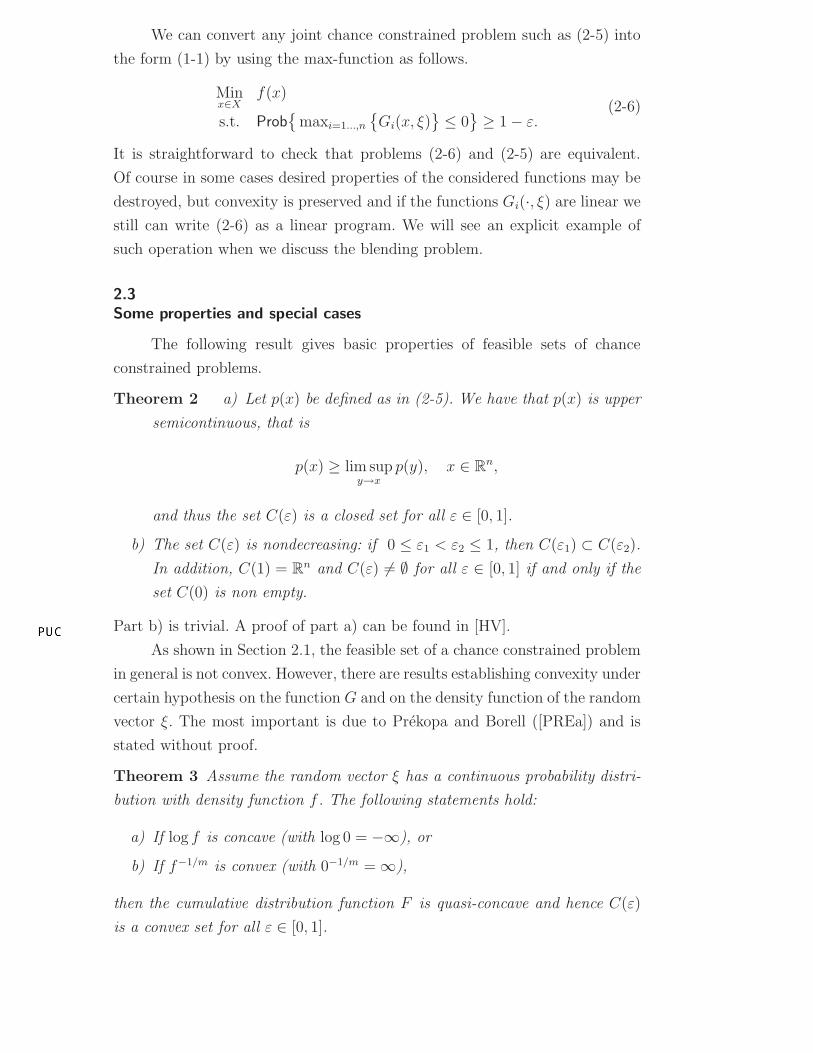
Theorem 2 a) Let p(x) be defined as in (2-5). We have that p(x) is upper

semicontinuous, that is

p(x) ≥ lim supy→x

p(y), x ∈ Rn,

and thus the set C(ε) is a closed set for all ε ∈ [0, 1].

b) The set C(ε) is nondecreasing: if 0 ≤ ε1 < ε2 ≤ 1, then C(ε1) ⊂ C(ε2).

In addition, C(1) = Rn and C(ε) 6= ∅ for all ε ∈ [0, 1] if and only if the

set C(0) is non empty.

Part b) is trivial. A proof of part a) can be found in [HV].

As shown in Section 2.1, the feasible set of a chance constrained problem

in general is not convex. However, there are results establishing convexity under

certain hypothesis on the function G and on the density function of the random

vector ξ. The most important is due to Prekopa and Borell ([PREa]) and is

stated without proof.

Theorem 3 Assume the random vector ξ has a continuous probability distri-

bution with density function f . The following statements hold:

a) If log f is concave (with log 0 = −∞), or

b) If f−1/m is convex (with 0−1/m = ∞),

then the cumulative distribution function F is quasi-concave and hence C(ε)

is a convex set for all ε ∈ [0, 1].

Fortunately, there are several important distributions that satisfy the hypothe-

sis of Theorem 3. We give two examples:

– Uniform distribution. Let D be a convex subset of Rn with finite measure

|D|. The probability density function is given by

f(x) =

{

1|D|

if x ∈ D,

0 if x /∈ D.

– Normal distribution. The probability density function is defined by

f(x) =1

√

|Σ|(2π)n

2

exp− 1

2(x−µ)T Σ−1(x−µ), x ∈ R

n,

where µ is the expectation vector, Σ the covariance matrix of the

distribution and |Σ| is the determinant of Σ.

Other examples are the (multivariate) Beta and Gamma distributions. More

examples can be found in [PREa].

In the case the random variable ξ is discretely distributed, we can

formulate problem (1-1) as a mixed-integer linear program. Let us assume

Prob{ξ = ξk} = pk, k = 1, . . . , K. Problem (1-1) becomes

Minx∈X

f(x)

s.t.∑K

k=1 pk1l(−∞,0)(G(x, ξk)) ≥ 1 − ε,(2-7)

or, equivalently,

Minx∈X

f(x)

s.t.∑K

k=1 pk1l(0,∞)(G(x, ξk)) ≤ ε,(2-8)

Consider the following mixed-integer program.

Minx∈X

f(x)

s.t. G(x, ξk) − Mzk ≤ 0, k = 1, . . . , K,∑K

k=1 pkzk ≤ ε,

z ∈ {0, 1}K,

(2-9)

where M is a sufficiently large constant. We claim that (2-8) and (2-9) are

equivalent. Indeed, let (x, z1, . . . , zk) be a solution of problem (2-9). The

first constraint of (2-9) tells us that zk ≥ 1l(0,∞)(G(x, ξk)). From the second

constraint of (2-9) we have

ε ≥K

∑

k=1

pkzk ≥K

∑

k=1

pk1l(0,∞)(G(x, ξk)),

which implies that x is feasible for (2-8), with same objective value. Conversely,

let x be feasible for problem (2-8) and define zk := 1l(0,∞)(G(x, ξk)). We have

that (x, z1, . . . , zk) is feasible for (2-9) with same objective value, and thus both

problems are equivalent.

We conclude with a convexity result for discrete distributions. A proof

can be found in [KW].

Proposition 4 Consider problem (2-5) with discrete distribution, that is, let

pk = Prob{ξ = ξk}, k = 1, . . . , K. Then for

ε < mink=1...,K

{pk}

the feasible set C(ε) is convex.

3

Sample Average Approximation

We have seen in Chapter 2 that chance constrained problems are usually

hard to solve and explicit solutions are only available in very particular cases.

The main idea of SAA is to replace the original problem by an approximate

problem obtained via sampling from the distribution of the original problem.

We claim that good candidate solutions and bounds on the true optimal

value can be obtained by solving such approximations. We start with the

theoretical background for the method, stating and proving consistency results.

The discussion follows [PAS].

3.1

Theoretical background for SAA

As stated in Chapter 1, we consider chance constrained problems

Minx∈X

f(x)

s.t. Prob{

G(x, ξ) ≤ 0}

≥ 1 − ε.(3-1)

In order to simplify the presentation we assume in this section that the

constraint function G : Rn × Ξ → R is real valued. Of course, a number

of constraints Gi(x, ξ) ≤ 0, i = 1, . . . , m, can be equivalently replaced by one

constraint with the max-function as discussed in (2-6). We assume that the

set X is closed, the function f(x) is continuous and the function G(x, ξ) is a

Caratheodory function, i.e., G(x, ·) is measurable for every x ∈ Rn and G(·, ξ)

continuous for a.e. ξ ∈ Ξ.

Problem (3-1) can be written in the following equivalent form

Minx∈X

f(x) s.t. p(x) ≤ ε, (3-2)

where

p(x) := P{G(x, ξ) > 0}.

Now let ξ1, . . . , ξN be an independent identically distributed (iid) sample of N

realizations of random vector ξ and PN := N−1∑N

j=1 ∆(ξj) be the respective

empirical measure. Here ∆(ξ) denotes measure of mass one at point ξ, and

hence PN is a discrete measure assigning probability 1/N to each point ξj,

j = 1, . . . , N . The sample average approximation pN(x) of function p(x) is

obtained by replacing the ‘true’ distribution P by the empirical measure PN .

That is, pN(x) := PN{G(x, ξ) > 0}. Let 1l(0,∞) : R → R be the indicator

function of (0,∞), i.e.,

1l(0,∞)(t) :=

{

1, if t > 0,

0, if t ≤ 0.

Then we can write that p(x) = EP [1l(0,∞)(G(x, ξ))] and

pN(x) = EPN[1l(0,∞)(G(x, ξ))] =

1

N

N∑

j=1

1l(0,∞)

(

G(x, ξj))

.

That is, pN(x) is equal to the proportion of times that G(x, ξj) > 0. The

problem, associated with the generated sample ξ1, . . . , ξN , is

Minx∈X

f(x) s.t. pN(x) ≤ γ. (3-3)

We refer to problems (3-2) and (3-3) as the true and SAA problems, respec-

tively, at the respective significance levels ε and γ. Note that, following [LA]

and [PAS], we allow the significance level γ ≥ 0 of the approximate problem to

be different from the significance level ε of the true problem. Next we discuss

the convergence of a solution of the SAA problem (3-3) to that of the true

problem (3-2) with respect to the sample size N and the significance level γ. A

convergence analysis of problem (3-3) has been given in [LA]. Here we present

complementary results under slightly different assumptions.

Recall that a sequence fk(x) of extended real valued functions is said to

epiconverge to a function f(x), written fke→ f , if for any point x the following

two conditions hold: (i) for any sequence xk converging to x one has

lim infk→∞

fk(xk) ≥ f(x), (3-4)

(ii) there exists a sequence xk converging to x such that

lim supk→∞

fk(xk) ≤ f(x). (3-5)

Note that by the (strong) Law of Large Numbers (LLN) we have that for any

x, pN(x) converges w.p.1 to p(x).

Proposition 5 Let G(x, ξ) be a Caratheodory function. Then the functions

p(x) and pN(x) are lower semicontinuous, and pNe→ p w.p.1. Moreover,

suppose that for every x ∈ X the set {ξ ∈ Ξ : G(x, ξ) = 0} has P -measure zero,

i.e., G(x, ξ) 6= 0 w.p.1. Then the function p(x) is continuous at every x ∈ X

and pN(x) converges to p(x) w.p.1 uniformly on any compact set C ⊂ X, i.e.,

supx∈C

|pN(x) − p(x)| → 0 w.p.1 as N → ∞. (3-6)

Proof. Consider function ψ(x, ξ) := 1l(0,∞)

(

G(x, ξ))

. Recall that p(x) =

EP [ψ(x, ξ)] and pN(x) = EPN[ψ(x, ξ)]. Since the function 1l(0,∞)(·) is lower

semicontinuous and G(·, ξ) is a Caratheodory function, it follows that the

function ψ(x, ξ) is random lower semicontinuous1 (see, e.g., [RW, Proposition

14.45]). Then by Fatou’s lemma we have for any x ∈ Rn,

lim infx→x p(x) = lim infx→x

∫

Ξψ(x, ξ)dP (ξ)

≥∫

Ξlim infx→x ψ(x, ξ)dP (ξ) ≥

∫

Ξψ(x, ξ)dP (ξ) = p(x).

This shows lower semicontinuity of p(x). Lower semicontinuity of pN (x) can

be shown in the same way.

The epiconvergence pNe→ p w.p.1 is a direct implication of Artstein and

Wets [AW, Theorem 2.3]. Note that, of course, |ψ(x, ξ)| is dominated by an

integrable function since |ψ(x, ξ)| ≤ 1.

Suppose, further, that for every x ∈ X, G(x, ξ) 6= 0 w.p.1, which

implies that ψ(·, ξ) is continuous at x w.p.1. Then by the Lebesgue Dominated

Convergence Theorem we have for any x ∈ X,

limx→x p(x) = limx→x

∫

Ξψ(x, ξ)dP (ξ)

=∫

Ξlimx→x ψ(x, ξ)dP (ξ) =

∫

Ξψ(x, ξ)dP (ξ) = p(x).

This shows that p(x) is continuous at x = x. Finally, the uniform convergence

(3-6) follows by a version of the uniform Law of Large Numbers (see, e.g.,

[SHA, Proposition 7, p.363]).

By lower semicontinuity of p(x) and pN(x) we have that the feasible

sets of the ‘true’ problem (3-2) and its SAA counterpart (3-3) are closed sets.

Therefore, if the set X is bounded (i.e., compact), then problems (3-2) and (3-

3) have nonempty sets of optimal solutions denoted, respectively, as S and SN ,

provided that these problems have nonempty feasible sets. We also denote by

ϑ∗ and ϑN the optimal values of the true and the SAA problems, respectively.

The following result shows that for γ = ε, under mild regularity conditions,

ϑN and SN converge w.p.1 to their counterparts of the true problem.

We make the following assumption.

(A) There is an optimal solution x of the true problem (3-2) such that for

any ε > 0 there is x ∈ X with ‖x− x‖ ≤ ε and p(x) < ε.

1Random lower semicontinuous functions are called normal integrands in [RW].

In other words the above condition (A) assumes existence of a sequence

{xk} ⊂ X converging to an optimal solution x ∈ S such that p(xk) < ε

for all k, i.e., x is an accumulation point of the set {x ∈ X : p(x) < ε}.

Proposition 6 Suppose that the significance levels of the true and SAA

problems are the same, i.e., γ = ε, the set X is compact, the function f(x) is

continuous, G(x, ξ) is a Caratheodory function, and condition (A) holds. Then

ϑN → ϑ∗ and D(SN , S) → 0 w.p.1 as N → ∞.

Proof. By the condition (A), the set S is nonempty and there is x ∈ X

such that p(x) < ε. We have that pN(x) converges to p(x) w.p.1. Consequently

pN(x) < ε, and hence the SAA problem has a feasible solution, w.p.1 for N

large enough. Since pN(·) is lower semicontinuous, the feasible set of the SAA

problem is compact, and hence SN is nonempty w.p.1 for N large enough. Of

course, if x is a feasible solution of an SAA problem, then f(x) ≥ ϑN . Since

we can take such point x arbitrary close to x and f(·) is continuous, we obtain

thatlim sup

N→∞

ϑN ≤ f(x) = ϑ∗ w.p.1. (3-7)

Now let xN ∈ SN , i.e., xN ∈ X, pN(xN ) ≤ ε and ϑN = f(xN). Since the

set X is compact, we can assume by passing to a subsequence if necessary that

xN converges to a point x ∈ X w.p.1. Also we have that pNe→ p w.p.1, and

hence

lim infN→∞

pN(xN ) ≥ p(x) w.p.1.

It follows that p(x) ≤ ε and hence x is a feasible point of the true problem,

and thus f(x) ≥ ϑ∗. Also f(xN ) → f(x) w.p.1, and hence

lim infN→∞

ϑN ≥ ϑ∗ w.p.1. (3-8)

It follows from (3-7) and (3-8) that ϑN → ϑ∗ w.p.1. It also follows that the

point x is an optimal solution of the true problem and consequently we obtain

that D(SN , S) → 0 w.p.1.

Condition (A) is essential for the consistency of ϑN and SN . Think, for

example, about a situation where the constraint p(x) ≤ ε defines just one

feasible point x such that p(x) = ε. Then arbitrary small changes in the

constraint pN(x) ≤ ε may result in that the feasible set of the corresponding

SAA problem becomes empty. Note also that condition (A) was not used in

the proof of inequality (3-8). Verification of condition (A) can be done by ad

hoc methods.

Suppose now that γ > ε. Then by Proposition 6 we may expect that with

increase of the sample size N , an optimal solution of the SAA problem will

approach an optimal solution of the true problem with the significance level

γ rather than ε. Of course, increasing the significance level leads to enlarging

the feasible set of the true problem, which in turn may result in decreasing

of the optimal value of the true problem. For a point x ∈ X we have that

pN(x) ≤ γ, i.e., x is a feasible point of the SAA problem, iff no more than γN

times the event “G(x, ξj) > 0” happens in N trials. Since probability of the

event “G(x, ξj) > 0” is p(x), it follows that

Prob{

pN(x) ≤ γ}

= B(

⌊γN⌋; p(x), N)

. (3-9)

Recall that by Chernoff inequality [CHE], for k > Np,

B(k; p,N) ≥ 1 − exp{

−N(k/N − p)2/(2p)}

.

It follows that if p(x) ≤ ε and γ > ε, then 1 − Prob{

pN (x) ≤ γ}

approaches

zero at a rate of exp(−κN), where κ := (γ − ε)2/(2ε). Of course, if x is an

optimal solution of the true problem and x is a feasible point of the SAA

problem, then ϑN ≤ ϑ∗. That is, if γ > ε, then the probability of the event

“ϑN ≤ ϑ∗” approaches one exponentially fast. By similar analysis we have

that if p(x) = ε and γ < ε, then probability that x is a feasible point of the

corresponding SAA problem approaches zero exponentially fast (cf., [LA]).

The above is a qualitative analysis. For a given candidate point x ∈ X,

say obtained as a solution of a SAA problem, we would like to validate its

quality as a solution of the true problem. This involves two questions, namely

whether x is a feasible point of the true problem, and if so, then what is the

optimality gap f(x)−ϑ∗. Of course, if x is a feasible point of the true problem,

then f(x) − ϑ∗ is nonnegative and is zero iff x is an optimal solution of the

true problem.

Let us start with verification of feasibility of x. For that we need to

estimate the probability p(x). We proceed by employing again the Monte Carlo

sampling techniques. Generate an iid sample ξ1, ..., ξN and estimate p(x) by

pN(x). Note that this random sample should be generated independently of

a random procedure which produced the candidate solution x, and that we

can use a very large sample since we do not need to solve any optimization

problem here. The estimator pN(x) of p(x) is unbiased and for large N and

not “too small” p(x) its distribution can be approximated reasonably well by

the normal distribution with mean p(x) and variance p(x)(1 − p(x))/N . This

leads to the following approximate (1 − β)-confidence upper bound on p(x):

Uβ,N(x) := pN(x) + zβ

√

pN(x)(1 − pN(x))/N. (3-10)

A more accurate (1 − β)-confidence upper bound is given by (cf., [NS]):

U∗

β,N(x) := supρ∈[0,1]

{ρ : B(k; ρ,N) ≥ β} , (3-11)

where k := NpN (x) =∑N

j=1 1l(0,∞) (G(x, ξj)).

In order to get a lower bound for the optimal value ϑ∗ we proceed as

follows. Let us choose two positive integers M and N , and let

θN := B(

⌊γN⌋; ε,N)

and L be the largest integer such that

B(L− 1; θN ,M) ≤ β. (3-12)

Next generate M independent samples ξ1,m, . . . , ξN,m, m = 1, . . . ,M , each of

size N , of random vector ξ. For each sample solve the associated optimization

problemMinx∈X

f(x)

s.t.∑N

j=1 1l(0,∞) (G(x, ξj,m)) ≤ γN,(3-13)

and hence calculate its optimal value ϑmN ,m = 1, . . . ,M . That is, solve M times

the corresponding SAA problem at the significance level γ. It may happen

that problem (3-13) is either infeasible or unbounded from below, in which

case we assign its optimal value as +∞ or −∞, respectively. We can view

ϑmN , m = 1, . . . ,M , as an iid sample of the random variable ϑN , where ϑN

is the optimal value of the respective SAA problem at significance level γ.

Next we rearrange the calculated optimal values in the nondecreasing order as

follows ϑ(1)N ≤ · · · ≤ ϑ

(M)N , i.e., ϑ

(1)N is the smallest, ϑ

(2)N is the second smallest

etc, among the values ϑmN , m = 1, . . . ,M . We use the random quantity ϑ

(L)N

as a lower bound of the true optimal value ϑ∗. It is possible to show that

with probability at least 1 − β, the random quantity ϑ(L)N is below the true

optimal value ϑ∗, i.e., ϑ(L)N is indeed a lower bound of the true optimal value

with confidence at least 1− β (see2 [NS]). We will discuss later how to choose

the constants M,N and γ based on numerical experiments.

2In [NS] this lower bound was derived for γ = 0. It is straightforward to extend thederivations to the case of γ > 0.

4

Two applications of SAA

In this Chapter we apply SAA to a portfolio problem and to a blending

problem. In the first the decision maker must choose the composition of a

portfolio of assets such that the expected return is maximized. Due to the

chance constraint, the total gain has to be greater than a pre-specified return

level v with high probability. When returns follow a multivariate normal

distribution, we compute the solution explicitly and compare it with the

results of SAA. When returns are lognormally distributed, we have to rely

on approximations.

The second problem is a joint version of a two dimensional blending

problem. We show that SAA can be readily applied to this situation at no

extra cost. Due to the independence assumption, we compute explicit answers

for this problem and use them as benchmarks to tune the parameters of SAA.

4.1

Portfolio problem

Consider the following maximization problem subject to a single chance

constraint:Maxx∈X

E[

rT x]

s.t. Prob{

rT x ≥ v}

≥ 1 − ε.(4-1)

Here x ∈ Rn is vector of decision variables, r ∈ R

n is a random vector

with known probability distribution, v ∈ R, ε ∈ (0, 1), e is a vector whose

components are all equal to 1 and

X := {x ∈ Rn : eT x = 1, x ≥ 0}.

Note that, of course, E[

rT x]

= µT x, where µ := E[r] is the corresponding

mean vector. That is, the objective function of problem (4-1) is linear and

deterministic.

The motivation to study (4-1) is the portfolio selection problem going

back to Markowitz [MAR]. The vector x represents the percentage of a total

wealth of one dollar invested in each of n available assets, r is the vector of

random returns of these assets and the decision agent wants to maximize the

mean return subject to having a return greater or equal to a desired level v,

with probability at least 1 − ε. In terms of risk measures, this requirement is

equivalent to a Value-at-Risk constraint. We note that problem (4-1) is not

realistic because it does not incorporate crucial features of real markets such

as cost of transactions, short sales, lower and upper bounds on the holdings,

etc. However, it will serve to our purposes as an example of an application

of the SAA method. For a more realistic model we can refer the reader, e.g.,

to [WCZ], where the authors include market frictions and discuss the best

distribution function for asset returns.

A very similar version of problem (4-1) was analyzed in [ZTSK], where the

authors obtained important information about the different policies available

in soil management as well as the trade off between net returns and soil loss.

We consider two different situations, namely when the vector of random

returns r follows multivariate normal and multivariate lognormal distributions.

The two cases are very distinct; on the former one can solve explicitly the

chance constraint, while in the latter no explicit formula is known. Under

normality, we can compare the quality of the approximations with the true

optimal value, while in the lognormal case we have to rely on approximations.

4.1.1

SAA of the portfolio problem

First assume that r follows a multivariate normal distribution with

mean vector µ and covariance matrix Σ, written r ∼ N (µ, Σ). In that case

rTx ∼ N(

µT x, xT Σ x)

, and hence (as it is well known) the chance constraint

in (4-1) can be written as a convex second order conic constraint (SOCC) as

follows.

Prob{

rTx ≥ v}

≥ 1 − ε ⇔

Prob

{

rT x − µT x√xT Σx

≥ v − µTx√xT Σx

}

≥ 1 − ε ⇔

1 − Prob

{

rT x − µT x√xT Σx

≤ v − µTx√xT Σx

}

≥ 1 − ε ⇔

1 − Φ

(

v − µT x√xT Σx

)

≥ 1 − ε ⇔

v − µT x√xT Σx

≤ z1−ε ⇔

v − µTx + z1−ε

√xT Σx ≤ 0. (4-2)

Using the explicit form (4-2) of the chance constraint, one can efficiently solve

the convex problem (4-1) for different values of ε. An efficient frontier of

portfolios can be constructed in an objective function value versus confidence

level plot, that is, for every confidence level ε we associate the optimal value

of problem (4-1). The efficient frontier dates back to Markowitz [MAR]. A

discussion of the subject can be found, e.g., in [CM].

If r follows a multivariate lognormal distribution, then no closed form

solution for the chance constrained problem (4-1) is available. The related

SAA problem (4-1) can be written as

Maxx∈X

µT x

s.t. pN(x) ≤ γ,(4-3)

where pN(x) := N−1∑N

i=1 1l(0,∞)(v − rTi x) and γ ∈ [0, 1). The reason we use γ

instead of ε is to suggest that for a fixed ε, a different choice of the parameter

γ in (4-3) might be suitable. For instance, if γ = 0, then the SAA problem

(4-3) becomes the linear program

Maxx∈X

µT x

s.t. rTi x ≥ v, i = 1, . . . , N .

(4-4)

A recent paper by Campi and Garatti [CG], building on the work of Calafiore

and Campi [CC], provides an expression for the probability of an optimal

solution xN of the SAA problem (3-3), with γ = 0, to be infeasible for the true

problem (3-2). That is, under the assumptions that the set X and functions

f(·) and G(·, ξ), ξ ∈ Ξ, are convex and that w.p.1 the SAA problem attains

unique optimal solution, we have that for N ≥ n,

Prob {p(xN) > ε} ≤ B(n − 1; ε, N), (4-5)

and the above bound is tight. We apply this bound to the considered portfolio

selection problem to conclude that for a confidence parameter β ∈ (0, 1) and

a sample size N∗ such that

B(n − 1; ε, N∗) ≤ β, (4-6)

the optimal solution of problem (4-4) is feasible for the corresponding true

problem (4-1) with probability at least 1 − β.

For γ > 0, problem (4-3) can be written as the mixed-integer linear

programMax

x,zµTx

s.t. rTi x + vzi ≥ v,

∑N

i=1 zi ≤ Nγ,

x ∈ X, z ∈ {0, 1}N ,

(4-7)

The equivalence of problems (4-3) and (4-7) was already proved when we

showed the equivalence of problems (2-8) and (2-9) in Chapter 2, Section 2.3.

Given a fixed ε in (4-1), it is not clear what are the best choices of γ and

N for approximation (4-7). We believe it is problem dependent and numerical

investigations will be performed with different values for both parameters. We

know from Proposition 6 that, for γ = ε the larger the N the closer we are to

the original problem (4-1). However, the number of samples N must be chosen

carefully because problem (4-7) is a binary problem. Even moderate values of

N can generate instances that are very hard to solve.

4.1.2

Obtaining candidate solutions

First we perform numerical experiments applying SAA to the portfolio

problem (4-1) assuming that r ∼ N (µ, Σ). We considered 10 assets (n = 10)

and the data for the estimation of the parameters was taken from historical

monthly returns adjusted for dividends from 1997 to 2007 of 10 US major

companies1. The sample was generated by the Triangular Factorization Method

[BS]. We wrote the codes in GAMS and solved the linear and binary problems

using CPLEX 9.0. The computer was a PC with an Intel Core 2 processor and

2GB of RAM.

Let us fix ε = 0.10 and β = 0.01. For these values, the sample size

suggested by (4-6) is N∗ = 183. We ran 10 independent replications of (4-4)

for each of the sample sizes N = 30, 40, . . . , 200 and for N∗ = 183. We also

build an efficient frontier plot of optimal portfolios with an objective value

versus Prob{rT xε ≥ v} axes, where xε is the optimal solution of problem (4-

1) for a given ε. We show in the same plot (Figure 4.1) the corresponding

objective function values and Prob{rT xN ≥ v} for each optimal solution xN

found for the problem (4-4). To identify each point with a sample size, we

used a gray scale that attributes light tones of gray to smaller sample sizes

and darker ones to larger samples. The efficient frontier curve is calculated for

ε = 0.8, 0.81, . . . , 0.99 and then connected by lines. The vertical and horizontal

lines are for reference only: they represent the optimal value for problem (4-1)

with ε = 0.10 and the 90% reliability level, respectively.

Figure 4.1 shows interesting features of the SAA problem (4-4). Although

larger sample sizes always generate feasible points, the value of the objective

function, in general, is quite small if compared with the optimal value 1.004311

of problem (4-1) with ε = 0.10. We also observe the absence of a convergence

property: if we increase the sample size, the feasible region of problem (4-4)

1JP Morgan, Oracle, Intel, Exxon, Wal-Mart, Apple, Sun Microsystems, Microsoft, Yahooand Procter & Gamble

0.80

0.85

0.90

0.95

1.00

0.998 1.004 1.010

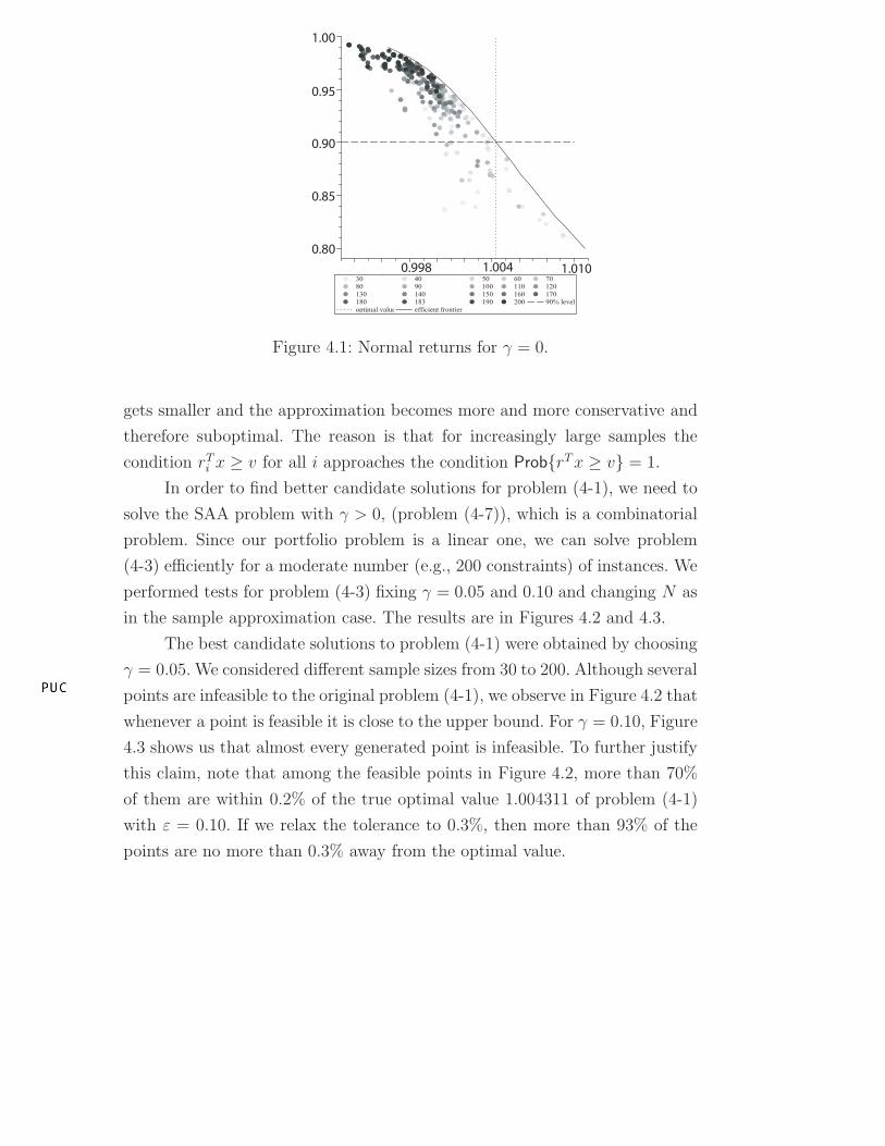
Figure 4.1: Normal returns for γ = 0.

gets smaller and the approximation becomes more and more conservative and

therefore suboptimal. The reason is that for increasingly large samples the

condition rTi x ≥ v for all i approaches the condition Prob{rT x ≥ v} = 1.

In order to find better candidate solutions for problem (4-1), we need to

solve the SAA problem with γ > 0, (problem (4-7)), which is a combinatorial

problem. Since our portfolio problem is a linear one, we can solve problem

(4-3) efficiently for a moderate number (e.g., 200 constraints) of instances. We

performed tests for problem (4-3) fixing γ = 0.05 and 0.10 and changing N as

in the sample approximation case. The results are in Figures 4.2 and 4.3.

The best candidate solutions to problem (4-1) were obtained by choosing

γ = 0.05. We considered different sample sizes from 30 to 200. Although several

points are infeasible to the original problem (4-1), we observe in Figure 4.2 that

whenever a point is feasible it is close to the upper bound. For γ = 0.10, Figure

4.3 shows us that almost every generated point is infeasible. To further justify

this claim, note that among the feasible points in Figure 4.2, more than 70%

of them are within 0.2% of the true optimal value 1.004311 of problem (4-1)

with ε = 0.10. If we relax the tolerance to 0.3%, then more than 93% of the

points are no more than 0.3% away from the optimal value.

0.80

0.85

0.90

0.95

1.00

1.000 1.005 1.0100.995

Figure 4.2: Normal with γ = 0.05.

0.80

0.85

0.90

0.95

1.00

1.000 1.0101.0050.995

Figure 4.3: Normal with γ = 0.10.

To investigate the possible choices of γ and N in problem (4-7), we

created a three dimensional representation which we call γN -plot. The domain

is a discretization of values of γ and N , forming a grid with pairs (γ, N). For

each pair we solve an instance of problem (4-7) with these parameters and

stored the optimal value and the approximate probability of being feasible to

the original problem (4-1). The z-axis represents the optimal value associated

to each point in the domain in the grid. Finally, we created a surface of triangles

based on this grid as follows. Let i be the index for the values of γ and j for the

values of N . If candidate points associated with grid members (i, j), (i + 1, j)

and (i, j + 1) or (i + 1, j + 1), (i + 1, j) and (i, j + 1) are feasible to problem

(4-1) (with probability greater than or equal to (1− ε)), then we draw a dark

gray triangle connecting the three points in the space. Otherwise, we draw a

light gray triangle.

We created a γN -plot for problem (4-1) with normal returns. The result

can be seen in Figure 4.4, where we also included the plane corresponding

to the optimal solution with ε = 0.10. The values for parameter γ were

0, 0.01, . . . , 0.10 and for N = 30, 40, . . . , 200. From Figure 4.4 we see that

for any fixed γ small sample sizes tend to generate infeasible solutions and

large samples feasible ones. As predicted by the results of Campi and Garatti,

when γ = 0, large sample sizes generate feasible solutions, although they can

be seen to be of poor quality judging by the low peaks observed in this region.

The concentration of high peaks corresponds to γ values around ε/2 = 0.05 for

almost all sample sizes, including small ones (varying from 50 until 120). We

generated different instances of Figure 4.4 and the output followed the pattern

described here.

1.005

1.0

0.995

30 80 130 1800.0

0.025

0.05

0.075

0.1

1.01

g

N

Figure 4.4: γN -plot for the portfolio problem with normal returns.

Even though there are peaks in other regions, Figure 4.4 suggests a

strategy to obtain good candidates for chance constrained problems: choose

γ close to ε/2, solve instances of SAA problems with small sizes of N (e.g. one

third of the Campi-Garatti estimate (4-6)) and keep the best solution. This

is fortunate because SAA problems with γ > 0 are binary problems that can

be hard to solve. Our experience with the portfolio problem and with others

suggest this strategy works better than trying to solve SAA problems with

large sample sizes. The choice γ = ε/2 came from our empirical experience.

We believe in general the choice of γ is problem dependent.

4.1.3

Upper bounds

A method to compute lower bounds of chance constrained problems of

the form (3-1) was suggested in [NS]. We summarized their procedure at the

end of Section 3.1, leaving the question of how to choose the constants L, M

and N . Given β, M and N , it is straightforward to specify L: it is the largest

integer that satisfies (3-12). For a given N , the larger M the better because we

are approximating the L-th order statistic of the random variable ϑN . However,

note that M represents the number of problems to be solved and this value is

often constrained by computational limitations.

In [NS] an indication of how N should be chosen is not given. It is possible

to gain some insight on the magnitude of N by doing some algebra in inequality

(3-12). With γ = 0, the first term (i = 0) of the sum (3-12) is

[

1 − (1 − ε)N]M ≈

[

1 − e−Nε]M

. (4-8)

Approximation (4-8) suggests that for small values of ε we should take N of

order O(ε−1). If N is much bigger than 1/ε then we would have to choose a very

large M in order to honor inequality (3-12). For instance if ε = 0.10, β = 0.01

and N = 100 instead of N = 1/ε = 10 or N = 2/ε = 20, we need M to be

greater than 100 000 in order to satisfy (3-12), which can be computationally

intractable for some problems. If N = 200 then M has to be grater then 109,

which is impractical for most applications.

In [LA], the authors applied the same technique to generate bounds on

probabilistic versions of the set cover problem and the transportation problem.

To construct the bounds they varied N and used M = 10 and L = 1. For many

instances they obtained lower bounds slightly smaller (less than 2%) or even

equal to the best optimal values generated by SAA. In the portfolio problem,

the choice L = 1 generated poor bounds as we will see.

We performed experiments for the portfolio problem with returns now

following a lognormal distribution. Figure 4.5 shows the sample points obtained

by SAA with γ = 0 and with the corresponding probability estimated by

Monte-Carlo. The reader is referred to [LK] for detailed instructions of how

to generate samples from a multivariate lognormal distribution. Since in the

lognormal case one cannot compute the efficient frontier, we also included in

Figure 4.5 upper bounds2 for ε = 0.02, . . . , 0.20, calculated according to (3-

12). We fixed β = 0.01 for all cases and chose three different values for the

constants L, M and N .

First we fixed L = 1 and N = ⌈1/ε⌉ (solid line in Figure 4.5, upper bound

A). The constant M was chosen to satisfy the inequality (3-12). The results

were not satisfactory, mainly because M ended up being too small. Since the

constant M defines the number of samples from vN and since our problem is

a linear one, we decided to fix M = 1 000. Then we chose N = ⌈1/ε⌉ (dashed

line in Figure 4.5, upper bound B) and defined L to be the largest integer such

that (3-12) is satisfied. Finally, we generated an upper bound with M = 1 000

and N = ⌈2/ε⌉ (dotted line in Figure 4.5, upper bound C).

It is harder to construct upper bounds with γ > 0. The difficulty lies

in solving integer problems and it is hard to find an appropriate choice of

the parameters M or N in order to keep the problem size manageable. Based

on experiments, a good choice for this problem is M = 500, N = 50 and

γ = ε/2 = 0.05, which originated the dotted upper bound in Figure 4.5.

Although it is slightly better than the bounds obtained with γ = 0, in many

situations one often wants an upper bound without much computational effort.

If that is the case, it might be appropriate to use equation (3-12) for γ = 0

2The portfolio problem (4-1) is a maximization problem.

0.80

0.85

0.90

0.95

1.00

1.021.011.00

Figure 4.5: Lognormal with γ = 0.

since the corresponding problems are easier to solve.

0.80

0.85

0.90

0.95

1.00

1.010 1.0301.020

Figure 4.6: Lognormal with γ =

0.05.

0.80

0.85

0.90

0.95

1.00

1.010 1.020 1.030

Figure 4.7: Lognormal with γ =

0.10.

Following the normal case, we performed similar experiments with γ =

ε/2 and γ = ε. The results are in Figures 4.6 and 4.7 respectively, where we

only included the dashed upper bound. The experiments for the lognormal

case confirmed the tendency observed in the normal case: γ = ε generated

infeasible points, γ = 0 generated feasible points of poor quality if measured

by the distance to the upper bound curves and γ = ε/2 yielded the best

candidate solutions.

4.2

A blending problem

Let us consider a second example of a chance constrained problem.

Suppose a farmer has some crop and wants to use fertilizers to increase the

production. He hires an agronomy engineer who recommends 7 g of nutrient

A and 4 g of nutrient B. He has two kinds of fertilizers available: the first has

ω1 g of nutrient A and ω2 g of nutrient B per kilogram. The second has 1 g of

each nutrient per kilogram. The quantities ω1 and ω2 are uncertain: we assume

they are (independent) continuous uniform random variables with support in

the intervals [1, 4] and [1/3, 1] respectively. Furthermore, each fertilizer has a

unitary cost per kilogram.

There are several ways to model this blending problem. A detailed

discussion can be found in [HV], where the authors use this problem to motivate

the field of stochastic programming. We consider a joint chance constrained

formulation as follows:

Minx1,x2

x1 + x2

s.t. Prob{ω1x1 + x2 ≥ 7, ω2x1 + x2 ≥ 4} ≥ 1 − ε,

x1, x2 ≥ 0,

(4-9)

where xi represents the quantity of fertilizer i purchased, i = 1, 2, and ε ∈ [0, 1]

is the reliability level. The independence assumption allows us to convert the

joint probability in (4-9) into a product of probabilities. After some tedious

calculations, one can explicitly solve (4-9) for all values of ε. For ε ∈ [1/2, 1]

the solution (x∗

1, x∗

2) and the optimal value v∗ = x∗

1 + x∗

2 are

x∗

1 =18

9 + 8(1 − ε), x∗

2 =2(9 + 28(1 − ε))

9 + 8(1 − ε), v∗ =

4(9 + 14(1 − ε))

9 + 8(1 − ε).

For ε ∈ [0, 1/2], v∗ is

v∗ =2(25 − 18(1 − ε))

11 − 9(1 − ε). (4-10)

Our goal is to exemplify the use of SAA to joint chance constrained

problems. In addition, we use problem (4-9) as a benchmark to gain more

understanding of tuning of the underlying parameters of the SAA approach

since an explicit solution is available in this case. As mentioned in Section

2.3 of Chapter 2, we can convert a joint chance constrained problem into a

problem of the form (3-1) using the min (or max) operators. Problem (4-9)

becomes

Minx1,x2

x1 + x2

s.t. Prob {min{ω1x1 + x2 − 7, ω2x1 + x2 − 4} ≥ 0} ≥ 1 − ε,

x1, x2 ≥ 0.

(4-11)

Introducing one auxiliary variable zi per scenario, it is possible to formulate the

SAA method to problem (4-11) as a mixed integer linear program as follows.

0.90

0.95

1.00

6.05.5 7.06.5 7.5

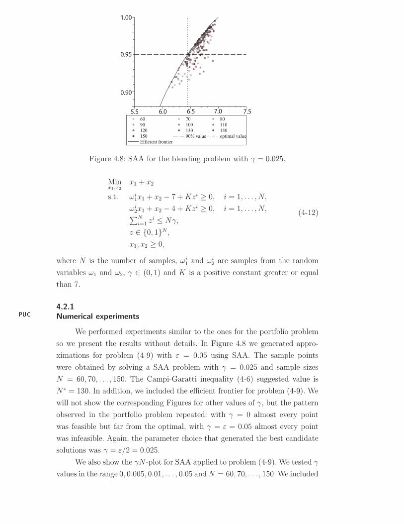
Figure 4.8: SAA for the blending problem with γ = 0.025.

Minx1,x2

x1 + x2

s.t. ωi1x1 + x2 − 7 + Kzi ≥ 0, i = 1, . . . , N,

ωi2x1 + x2 − 4 + Kzi ≥ 0, i = 1, . . . , N,

∑N

i=1 zi ≤ Nγ,

z ∈ {0, 1}N ,

x1, x2 ≥ 0,

(4-12)

where N is the number of samples, ωi1 and ωi

2 are samples from the random

variables ω1 and ω2, γ ∈ (0, 1) and K is a positive constant greater or equal

than 7.

4.2.1

Numerical experiments

We performed experiments similar to the ones for the portfolio problem

so we present the results without details. In Figure 4.8 we generated appro-

ximations for problem (4-9) with ε = 0.05 using SAA. The sample points

were obtained by solving a SAA problem with γ = 0.025 and sample sizes

N = 60, 70, . . . , 150. The Campi-Garatti inequality (4-6) suggested value is

N∗ = 130. In addition, we included the efficient frontier for problem (4-9). We

will not show the corresponding Figures for other values of γ, but the pattern

observed in the portfolio problem repeated: with γ = 0 almost every point

was feasible but far from the optimal, with γ = ε = 0.05 almost every point

was infeasible. Again, the parameter choice that generated the best candidate

solutions was γ = ε/2 = 0.025.

We also show the γN -plot for SAA applied to problem (4-9). We tested γ

values in the range 0, 0.005, 0.01, . . . , 0.05 and N = 60, 70, . . . , 150. We included

6.95

5.45

6.45

5.95

0.025

0.05

0.075

0.1

120

100

60

140

80

N

g

Figure 4.9: γN -plot for the blending problem.

a plane representing the optimal value of problem (4-9) for ε = 0.05, which is

readily obtained by applying formula (4-10).

In accordance with Figure 4.4, we note that in Figure 4.9 the best

candidate solutions are the ones with γ around 0.025. Even for very small

sample sizes we have feasible solutions (dark gray triangles) relatively close to

the optimal plane. On the other hand, this experiment gives more evidence that

SAA with γ = 0 is excellent to generate feasible solutions (dark gray triangles)

but the quality of the solutions is poor. As shown in Figure 4.9, the high peaks

associated with γ = 0 persist for any sample size, generating points far form

the optimal plane. In agreement with Figure 4.4, the candidates obtained for

γ close to ε were mostly infeasible.

5

From separated to joint variables: the hurdle-race problem

We consider a general provisioning problem, where an economic agent

aims to determine an initial amount that would be needed in order to meet

a series of future payment obligations with a sufficiently large probability. We

assume a “hold-to-maturity” (actuarial) approach: the initial provision is such

that upon investing it in a portfolio one is always able in the future to pay-

off the cash flows. In contrast, the “available-for-sales” (financial) framework

admits the possible fall in the arbitrage-free price of the series of cash flows

over a given time period and use it as means of assessing risk and establishing

buffers. Although the latter approach is at the core of the latest regulatory

documents such as Basel II and Solvency II, it can induce crashes when they

would not otherwise occur. Furthermore, we believe better risk measures are

available, such as the so-called coherent risk measures [ADEH]. This does not

mean that the financial approach is wrong but the actuarial framework is at

least a complementing alternative. For a detailed criticism of those regulatory

documents we refer the reader to [DEGK].

In [VDGK], the authors study the provisioning problem and impose

minimum requirements of available capital at each period, called hurdles. In

their framework, hurdles are modeled as separated chance constraints with

given reliability levels, one for each period of time. They coined the term hurdle-

race problem to describe the provisioning problem with hurdles. We start by

summarizing the approach proposed in [VDGK] and stating their main result.

Then we propose an alternative chance constrained model which requires that

all the obligations should be met jointly with a given reliability level. To this

end we make use of a joint chance constraint and refer to the problem as

the joint hurdle-race problem. We propose to solve the corresponding problem

using SAA and to compare the results with [VDGK]. In addition, we consider

another generalization in which the hurdles are not determined by the model

builder but are defined as discounted values of future obligations by stochastic

risk-free rates.

5.1

The hurdle-race problem and comonotonicity

An insurer wants to determine the initial provision R0 required to meet

n future obligations, of costs α1, . . . , αn at fixed, prescribed times t1, . . . , tn, for

t ∈ [0, tn]. Among obligations, the insurer may invest his capital, with random

returns. More precisely, the stochastic return process (Y1, . . . , Yn) such that 1

unit at time 0 grows to exp(Y1 + · · ·+ Yj) at time tj determines the evolution

of capital Rj in time,

Rj = Rj−1 exp(Yj) − αj , j = 1, . . . , n. (5-1)

In [VDGK], the authors impose probabilistic constraints (the hurdles) that

have to be met every time tj, that is, provision Rj has to be larger than a

deterministic value Vj with high probability 1−εj. They formulate the hurdle-

race problem as follows:

R0 = MinR0≥V0

R0 (5-2)

Prob{Rj ≥ Vj |R0} ≥ 1 − εj , j = 1, . . . , n

for given hurdles V0, V1, . . . , Vn and given tolerances ε1, ε2, . . . , εn ∈ [0, 1].

To determine the optimal provision R0 in (5-2) set

S[0,j] =

j−1∑

i=1

αi exp(−Y1 − · · · − Yi) + (Vj + αj) exp(−Y1 − · · · − Yj), (5-3)

the stochastically discounted value of the future obligations in the restricted

time period [0, j]. Theorem 1 in [VDGK], below, gives the optimal solution of

problem (5-2) in terms of the quantiles of the distributions of S[0,j].

Theorem 7 The optimal initial provision R0 defined in (5-2) is given by

R0 = Max{V0, F−1S[0,1]

(1 − ε1), F−1S[0,2]

(1 − ε2), . . . , F−1S[0,n]

(1 − εn)},

where FS[0,j]is the cumulative distribution function of S[0,j], j = 1, . . . , n.

A basic ingredient in the proof is the simple fact that

Prob {Rj ≥ Vj | R0} = Prob{

S[0,j] ≤ R0

}

, j = 1, . . . , n.

Thus, in order to determine the optimal R0 we are led to compute the quan-

tiles of the random variables S[0,j], which is very hard in most relevant cases.

For instance, if the random return process (Y1, . . . , Yn) follows a multivariate

normal distribution, we have that S[0,j] is a sum of lognormal distributions, a

random variable with no known distribution. The approach in [VDGK] repla-

ces the random variables S[0,j] by simpler random variables using comonotonic

approximations, whose quantiles can be calculated explicitly. Such approxima-

tions assume the random vector is strongly correlated, with all the components

depending on the same univariate random variable. A detailed description of

the theory of comonotonicity can be found in [DDGa]. For examples and ap-

plications we refer the reader to [DDGb].

In [VDGK], numerical experiments are performed for the case in which

the random variables (5-3) are sums of lognormals, and hence the return

process (Y1, . . . , Yn) follows a multivariate normal distribution. They compare

their results with the values obtained from the empirical distribution of S[0,j].

In the next section, in the more general joint hurdle-race problem, we apply

SAA to obtain good candidate solutions. We compare the results for the joint

hurdle-race to the ones obtained in [VDGK]. From now on we refer to this

model (5-2) as the separated hurdle-race problem.

5.2

The joint hurdle-race problem

The definition of R0 in (5-2) does not reflect the proper safety requi-

rements: for each fixed time tj the probability of not satisfying a hurdle is

small, but the probability of having missed one of the hurdles may remain

high. Indeed, there is no guarantee that the optimal provision keeps the joint

probability of missing at least one hurdle low. In [HEN], the author exempli-

fies the contrast between both models in a cash matching problem somewhat

similar to the separated hurdle race problem (5-2).

We then consider the joint hurdle-race problem,

R0 = MinR0≥V0

R0 (5-4)

Prob{Rj ≥ Vj, j = 1, . . . , n |R0} ≥ 1 − ε (5-5)

for ε ∈ [0, 1]. As opposed to problem (5-2), the optimal provision R0 in problem

(5-4) is the smallest value such that with high probability no hurdle is violated.

Although we have a single constraint in (5-4) opposed to n constraints

in (5-2), problem (5-4) is harder to solve: the joint probability calculation in

(5-4) involves the computation of a quantile of the cumulative distribution

of the random vector (S[0,1], S[0,2], . . . , S[0,n]), an extremely difficult task. Even

checking feasibility for a given candidate R0 is usually hard.

We use SAA to obtain good candidate solutions of (5-4) and lower bounds

for the optimal value. Indeed, (5-4) is a joint chance constrained problem so

the techniques of the previous Chapters apply.

The joint hurdle-race problem is not explicitly written in format (1-1),

but it can be easily converted by employing the max-function

Prob {R1 ≥ V1, . . . , Rn ≥ Vn|R0} = Prob{

S[0,1] ≤ R0, . . . , S[0,n] ≤ R0

}

= Prob

{

maxj=1,...,n

{S[0,j]} ≤ R0

}

= Prob

{

maxj=1,...,n

{S[0,j]} − R0 ≤ 0

}

. (5-6)

Using (5-6) we have that problem (5-4) is a particular case of (1-1):

MinR0≥V0

R0

s.t. Prob

{

maxj=1,...,n

{S[0,j]} − R0 ≤ 0

}

≥ 1 − ε.(5-7)

But how do we solve (5-7) with SAA? Given a sample size N and a reliability

level γ, the SAA formulation becomes a MILP as follows.

MinR0≥V0

R0

s.t. (V1 + α1) exp(−Y s1 ) − R0 − Kzs ≤ 0, s = 1, . . . , N,

...∑j

i=1 αi(j) exp(−Y s1 − · · · − Y s

i ) − R0 − Kzs ≤ 0, s = 1, . . . , N,...

∑n

i=1 αi(n) exp(−Y s1 − · · · − Y s

n ) − R0 − Kzs ≤ 0, s = 1, . . . , N,∑N

s=1 zs ≤ Nγ,

zs ∈ {0, 1}N ,

(5-8)where K is a sufficiently large positive constant, Y s

i are samples from the return

process (Y1, . . . , Yn) and

αi(j) =

{

αi, i 6= j,

Vj + αj , i = j.

The feasibility check cannot be performed exactly and uses Monte-Carlo

methods.

5.2.1

Numerical experiments

We compare separated and the joint hurdle-race problems. Following

[VDGK], we performed experiments with n = 40 periods of investment and

with normal iid returns Yi with mean µ = log 1.10 and standard deviation

σ = 0.10. The hurdles and the liabilities are equal to 10 and 0.8 respectively for

all time periods. For the separated hurdles we choose εj = 0.05 for all periods

and for the joint case we take ε = 0.05. Our numerical experiments showed that

the stochastic lower bound approximation in [VDGK] is extremely accurate

for the separated hurdle-race problem, and we obtained R0 = 13.56411337.

An (stochastic) upper bound, obtained by the comonotonic approximation, is

14.48125099.

For the joint hurdle-race problem, we first choose values of γ and N .

Following the empirical findings for the portfolio problem and the blending

problem of the previous Chapter, we set γ = ε/2 = 0.025. We then compute

the value of N for which the optimal solution of the SAA problem is feasible

for the original problem with probability greater than 99% (see [CG]), which

in this case is N = 90. This estimate is usually too conservative and should

be regarded as an upper bound for the actual value of N to be used in the

experiments. The best result was obtained for N = 50 and the smallest initial

provision was R0 = 15.81238194. A Monte-Carlo experiment with 100 000

samples estimated the true probability of this candidate as 0.9527 and it is

thus feasible for the original problem.

We compute statistical lower bounds for the optimal value of the joint

hurdle-race problem following section 4.1.3. Fixing M = 1 000 and L according

to (3-12), the 99%-confidence lower bound for the optimal value is 15.302594.

Obviously, the candidate solution obtained by SAA can be regarded as an

upper bound for the true optimal value (if feasible).

Similar experiments were performed with εj = 0.01. The techniques in

[VDGK] give 16.34858684 for the solution of the separated problem, with

comonotonic upper bound1 equal to 18.37208466. It is not clear how these

methods should be extended to the joint hurdle problem. In this case, applying

SAA with N = 150 and γ = ε/2 = 0.005, the new method obtained

18.21640345. The true probability was estimated by Monte-Carlo and was

equal to exactly 1, with 100 000 samples. The 99%-confident lower bound

obtained was 17.515987.

It is interesting to compare the solution for the joint case (5-4) with the

one for the separate case (5-2). The best provisions obtained for the latter were

less than those for the former in both experiments. One might be tempted to

adopt the separated version as the best model since smaller provisions are

usually preferred. However, the solution of the joint problem is obviously more

robust. We proceed to substantiate this claim with some simulations.

The separated case was treated as in [VDGK], whereas we used SAA

for the joint problem. For illustration, we first present small size simulation

1The comonotonic upper bound is constructed using conditional expectations of como-

notonic random variables.

experiments that show the differences between the two approaches. Figures

5.1 and 5.2 show the estimated probability of violating each hurdle for the

separated problem. The values in the y-axis are close to 0.05 and 0.01

respectively, in accordance with the chosen reliability levels. Figures 5.3 and

5.4 show 100 sample paths for each choice of ε in the separated case. In Figure

5.3, 12 paths violated one of the hurdles at least once, giving a violation

probability of 0.12, significantly higher than the original 0.05 confidence level.

In Figure 5.4, the probability of violation was 0.06, also higher than the original

significance level 0.01. In the joint case, Figures 5.5 and 5.6 indicate that at

least one constraint was violated only 3% and 1% of the time, in accordance

with the joint reliability levels ε = 0.05 and ε = 0.01, a much more robust

situation.

In order improve numerical accuracy, we ran the same experiments for

10 000 paths. For εj = ε = 0.05, the estimated probability of violation of

at least one hurdle for the separated hurdle-race problem was 0.1173, much

higher than the corresponding value 0.0328 for the joint version with the same

reliability level. For εj = ε = 0.01, the estimated values were 0.0247 for the

separated formulation and 0.0094 for the joint counterpart. In both cases the

separated hurdle-race problem misses the joint reliability level by roughly twice

the pre-determined reliability level, substantially underestimating the more

robust provision given by SAA for the joint case.

0 5 10 15 20 25 30 35 40 450

0.01

0.02

0.03

0.04

0.05

0.06

0.07

0.08

Figure 5.1: ε = 0.05.

0 5 10 15 20 25 30 35 40 450

0.005

0.01

0.015

0.02

0.025

0.03

0.035

0.04

Figure 5.2: ε = 0.01.

5.3

Stochastic hurdles

We now consider a joint hurdle-race model with the possibility of mo-

deling stochastic hurdles. Now we define the hurdles as the market consistent

value of future liabilities when evaluating the portfolio at period j, i.e., the

0 5 10 15 20 25 30 35 40 45−200

0

200

400

600

800

1000

1200

Figure 5.3: Sample paths for ε =0.05, SHR.

0 5 10 15 20 25 30 35 40 45

0

500

1000

1500

2000

2500

3000

Figure 5.4: Sample paths for ε =0.01, SHR.

0 5 10 15 20 25 30 35 40 45

0

500

1000

1500

2000

2500

Figure 5.5: Sample paths for ε =0.05, JHR.

0 5 10 15 20 25 30 35 40 45

0

200

400

600

800

1000

1200

1400

1600

1800

Figure 5.6: Sample paths for ε =0.01, JHR.

hurdles will be the discounted cash flows at the stochastic risk-free rate. In

particular, the hurdles Vj are not known at period j.

In addition to the stochastic return process (Y1, . . . , Yn), the model will

have a risk-free rate process (r1, . . . , rn) that will determine the (stochastic)

hurdles as follows.

V0 = α1 exp(−r1) + α2 exp(−r1 − r2) + · · ·+ αn exp(−r1 − · · · − rn),

V1 = α1 + α2 exp(−r2) + · · ·+ αn exp(−r2 − · · · − rn),

... (5-9)

Vn = αn.

SAA obtains candidate solutions with no additional computational effort.

In the numerics, the risk-free rate process was composed of iid normal random

variables with mean µr = 0.04 and standard deviation σr = 0.05. The

stochastic return process is the same as described in section (5.2.1). For

ε = 0.05, the best solution was 21.68791898, with N = 60 and γ = ε/2 = 0.025.

The estimated probability was 0.95275, using 20 000 samples. For ε = 0.01,

the best solution was 25.17916015, with N = 120 and γ = ε/2 = 0.005. The

estimated probability was exactly 1, with 20 000 samples.

6

Conclusion

We believe that the SAA method is a valuable tool to obtain good

candidate solutions for chance constrained problems. An important advantage

of the method is the fairly general assumption on the underlying distribution

of the random variables of the problem: SAA only requires the ability to

sample from the given distribution. The related numerical analysis is tractable

and stable, allowing for practical implementations. The thesis bridges the

gap between theory and application, by presenting theoretical foundations,

techniques for parameter calibration and a collection of applications, which

exemplify as benchmarks and as new amenable problems.

SAA was used in a portfolio chance constrained problem with random

returns. In the normal case, the efficient frontier can be computed explicitly

and we used it as a benchmark solution. Fixing the parameters ε = 0.10 and

γ = 0 in the method, we concluded that the sample size suggested by Campi-

Garatti inequality (4-6) was too conservative for our problem: a much smaller

sample gave rise to better feasible solutions. Similar results were obtained

for the lognormal case, where upper bounds were computed using a method

developed in [NS].

As another illustration of the SAA method, we modeled a two dimen-

sional blending problem as a joint chance constrained problem. Due to the

independence assumption, one can again solve the problem explicitly and find

the optimal solution for any given reliability level. This served as a benchmark

for SAA on the class of approximate joint chance constrained problems.

In both examples, the choice γ = ε/2 obtains very good candidate

solutions. Even though it generated more infeasible points if compared to the

choice γ = 0, the feasible ones were of better quality. Using the γN -plot

(Figures (4.4) and (4.9)) we were able to confirm these empirical findings for

our two test problems. Relatively small sample sizes (e.g., if compared to (4-6)

estimates) can yield good candidate solutions, which is crucial since for γ > 0

the SAA problem is an integer program. Upper bounds were constructed for

the portfolio problem with γ = 0 and continuous linear programs were solved

to obtain the estimates. According to approximation (4-8), the number of

samples N should be of order 1/ε. Since no closed solution is available for

the portfolio problem with lognormal returns, having an upper bound is an

important information about the variability of the solution.

Finally we described the hurdle-race problem, proposed in [VDGK]. We

proposed a more adequate formulation in which the hurdles were taken jointly.

We obtained good candidate solutions and lower bounds for the true optimal

value using SAA. An additional extension, assuming stochastic hurdles instead

of deterministic ones, is handled by SAA at almost no extra cost.

Future work will include writing a SAA solver. For this goal, the empirical

findings in this text are crucial. Together with H. Bortolossi, we started to write

a program in C++ using Osi, a uniform API for interacting with callable solver

libraries. At present, we handle SAA problems with SYMPHONY, an open-

source generic MILP developed by T.K. Ralphs. Both Osi and SYMPHONY

can be freely downloaded at www.coin-or.org. The idea is to make our solver

freely available for use with SLP-IOR1, a user-friendly interface for stochastic

programs developed by P. Kall and J. Mayer. As of yet, problems such as

the portfolio problem of Chapter 4, where the uncertainty is multiplying the

decision variables, cannot be solved by any solver available at SLP-IOR.

The first Chapters of the thesis, in a condensed form, are the content

to [PAS]. A text with S. Vanduffel about the hurdle-race problem is in prepa-

ration. We plan to extend the results described here by assuming stochastic

liabilities of the type

αi = ai + fi(Ei), i = 1, . . . , n,

where ai are constants, (E1, . . . , En) is a multivariate normal vector and fi

are given functions. Such a setting may be appropriate in the context of life

insurance activities. The ai would be the total amount of fixed guaranteed

benefits to be paid to the policy holders. The insurance company may also

provide a profit sharing mechanism linked to some return process (E1, . . . , En)

of an external benchmark (e.g a stock index).

1 www.ior.uzh.ch/Pages/English/Research/StochOpt/index en.php

Bibliography

[AHM] AHMED, S. Convexity and decomposition of mean-risk sto-

chastic programs. Mathematical Progamming, v. 106, p. 433–446,

2006.

[AW] ARTSTEIN, Z.; WETS, R.J.-B. Consistency of minimizers and

the slln for stochastic programs. Journal of Convex Analysis,

v. 2, p. 1–17, 1996.

[ADEH] ARTZNER, P.; DELBAEN, F.; EBER, J-.M.; HEATH, D. Cohe-

rent measures of risk. Mathematical Finance, v. 9, p. 203–228,

1999.

[BS] BARR, D.R.; SLEZAK, N.L. A comparison of multivariate

normal generators. Communications of the ACM, v. 15, p. 1048–

1049, 1972.

[BEA] BEALE, E.M.L. On minimizing a convex function subject to

linear inequalities. Journal of the Royal statistical Society, Series

B, v. 17, p. 173–184, 1955.

[BN] BEN-TAL, A.; NEMIROVSKI, A. Robust optmization –

methodology and applications. Mathematical Programming, v.

93, p. 453–480, 2002.

[BP] BORTOLOSSI, H.J.; PAGNONCELLI, B. Uma

introducao a otimizacao sob incerteza. III

Bienal da SBM, Goiania, Brazil. Available at

http://www.mat.puc-rio.br/∼hjbortol/seminarios

/2006.1/soe/arquivos/iii-bienal-sbm-texto.pdf, 2006.

[CC] CALAFIORE, G.; CAMPI, M.C. The scenario approach to

robust control design. IEEE Transactions on Automatic Control,

v. 51, p. 742–753, 2006.

[CCS] CHARNES, A.; COOPER, W. W.; SYMMONDS, G.H. Cost ho-

rizons and certainty equivalents: an approach to stochastic

programming of heating oil. Management Science, v. 4, p. 235–

263, 1958.

[CG] CAMPI, M.C.; GARATTI, S. The exact feasibility of rando-

mized solutions of robust convex programs. Available at Op-

timization online (www.optimization-online.org), 2007.

[CHE] CHERNOFF, H. A measure of asymptotic efficiency for tests

of a hypothesis based on the sum observations. Annals of

Mathematical Statistics, v. 23, p. 493–507, 1952.

[CM] CONSTANTINIDES, G.; MALLIARIS, A.G. Portfolio theory. In

R.A. Jarrow, V. Maksimovic, and W.T. Ziemba, editors, Finance, v.

9 of Handbooks in OR & MS, North-Holland Publishing Company,

p. 1–30, 1995.

[DEGK] DANIELSSON, J. et al. An academic response to Basel II.

LSE Financial Markets Group, Special Paper Series, number 130,

2001.

[DAN] DANTZIG, G.B. Linear programming under uncertainty.

Management science, vol. 1, 197–206, 1955.

[DPR] DENTCHEVA, D.; PREKOPA, A.; RUSZCZYNSKI, A. Conca-

vity and efficient points of discrete distributions in pro-

babilistic programming. Mathematical Programming, v. 89, p.

55–77, 2000.

[DDGa] DHAENE, J. et al. The concept of comonotonicity in actu-

arial science and finance: theory. Insurance: Mathematics and

Economics, v. 31, p. 3–33, 2002.

[DDGb] DHAENE, J. et al. The concept of comonotonicity in actua-

rial science and finance: applications. Insurance: Mathematics

and Economics, v. 31, p. 133–161, 2002.

[DGKS] DUPACOVA, J.; GAIVORONSKI, A.; KOS, Z.; SZANTAI, T. Sto-

chastic programming in water management: a case study

and a comparison of solution techniques. European Journal

of Operational Research, v. 52, p. 28–44, 1991.

[HV] KLEIN HANEVELD, W.K.; VAN DER VLERK, M.H. Stochastic

Programming (lecture notes). 2007.

[HEN] HENRION, R. Introduction to chance constrained program-

ming. Available at http://www.stoprog.org/.

[HM] HENRION, R.; MOLLER, A. Optimization of a continuous

distillation process under random inflow rate. Computers &

Mathematics with Applications, v. 45, p. 247–262, 2003.

[HLMS] HENRION, R. et al. Stochastic optimization for opera-

ting chemical processes under uncertainty. In Grtschel, M.,

Krunke, S., Rambau, J., (editors), Online optimization of large scale

systems, Springer, p. 457–478, 2001.

[HS] HIGLE, J.; SEN, S. Stochastic Decomposition: A Statistical

Method for Large Scale Stochastic Linear Programming.

Springer, Berlin, 1996.

[KM] KALL, P.; MAYER, J. Stochastic Linear Programming. Sprin-

ger, 2005.

[KW] KALL, P.; WALLACE, S. Stochastic Programming. Wiley John

& Sons, 1995. Freely available at http://www.stoprog.org/.

[KQ] KAO, E.P.C.; QUEYRANNE, M. Budgeting cost of nursing in

a hospital. Management Science, v. 31, p. 608–621, 1985.

[LSW] LINDEROTH, J.; SHAPIRO, A.; WRIGHT, S. The empirical

behavior of sampling methods for stochastic programming,

Annals of Operations Research, v. 142, p. 215–241, 2006.

[LS] LOUVEAUX, F.V.; SMEERS, Y. Optimal investments for elec-

tricity generation: a stochastic model and a test problem.

In Yu. Ermoliev and R.J.-B. Wets, editors, Numerical techniques for

stochastci optimization, chapter 24, Springer-Verlag, Berlin, 1988.

[LA] LUEDTKE, J.; AHMED, S. A sample approximation approach

for optimization with probabilistic constraints SIAM Journal of

Optimization, v. 19, p. 674–699, 2008.

[LAN] LUEDTKE, J.; AHMED, S.; NEMHAUSER, G.L. An integer

programming approach for linear programs with proba-

bilistic constraints. To appear in Mathematical Programming,

2007.

[LK] LAW, A.; KELTON, W.D. Simulation Modeling and Analysis.

Industrial Engineering and Management Science Series. McGraw-

Hill Science/Engineering/Math, 1999.

[MAR] MARKOWITZ, H. Portfolio selection. Journal of Finance, v. 7,

p. 77–97, 1952.

[NS] NEMIROVSKI, A.; SHAPIRO, A.: Convex approximations of

chance constrained programs. SIAM Journal on Optimization,

v. 17, 969–996, 2006.

[PAS] PAGNONCELLI, B.K.; AHMED, S.; SHAPIRO, A. The Sample

Average Approximation method for chance constrained

programming: theory and applications. To appear in Journal

of Optimization Theory and Appplications, 2009.

[PP] PEREIRA, M.V.F.; PINTO, L.M.V.G. Multi-stage stochastic

optimization applied to energy planning. Mathematical Pro-

gramming, v. 52, p. 359–375, 1991.

[PBK] PETERS, R.J.; BOSKMA, K.; KUPPER, H.A.E. Stochastic pro-

gramming in production planning: a case with non-simple

recourse. Statistica Neerlandica, v. 31, p. 113–126, 1977.

[PREa] PREKOPA, A. Probabilistic programming. In A. Ruszczynski

and A. Shapiro, editors, Stochastic Programming, volume 10 of

Handbooks in OR & MS, North-Holland Publishing Company, p.

267-351, 2003.

[PREb] PREKOPA, A. Stochastic Programming. Kluwer Acad. Publ.,

Dordrecht, Boston, 1995.

[RW] ROCKAFELLAR, R.T.; WETS,R.J.-B. Variational Analysis.

Springer, Berlin, 1998.

[SHA] SHAPIRO, A. Monte carlo sampling methods. In

A. Ruszczynski and A. Shapiro, editors, Stochastic Program-

ming, volume 10 of Handbooks in OR & MS, North-Holland

Publishing Company, p. 353–425, 2003.

[SR] SHAPIRO, A.; RUSZCZYNSKI, A. Lectu-

res on stochastic programming. Available at

http://www2.isye.gatech.edu/~ashapiro/publications.html,

2008.

[VAN] VANDUFFEL, S. Comonotonicity: from risk measurement to

risk management. PhD thesis, University of Amsterdam, 2005.

[VDGK] VANDUFFEL, S., DHAENE, J., GOOVAERTS, M., KASS, R. The

hurdle-race problem. Insurance: Mathematics and Economics, v.

33, p. 405–413, 2003.

[WCZ] WANG, Y.; CHEN, Z.; ZHANG, K. A chance-constrained port-

folio selection problem under t-distrbution. Asia Pacific Jour-

nal of Operational Research, v. 24, p. 535–556, 2007.

[ZTSK] ZHU, M.; TAYLOR, D.B.; S. C. SARIN, S.C.; KRAMER, R.A.

Chance constrained programming models for risk-based

economic and policy analysis of soil conservation. Agricul-

tural and Resource Economics Review, v. 23, p. 58–65, 1994.

Livros Grátis( http://www.livrosgratis.com.br )

Milhares de Livros para Download: Baixar livros de AdministraçãoBaixar livros de AgronomiaBaixar livros de ArquiteturaBaixar livros de ArtesBaixar livros de AstronomiaBaixar livros de Biologia GeralBaixar livros de Ciência da ComputaçãoBaixar livros de Ciência da InformaçãoBaixar livros de Ciência PolíticaBaixar livros de Ciências da SaúdeBaixar livros de ComunicaçãoBaixar livros do Conselho Nacional de Educação - CNEBaixar livros de Defesa civilBaixar livros de DireitoBaixar livros de Direitos humanosBaixar livros de EconomiaBaixar livros de Economia DomésticaBaixar livros de EducaçãoBaixar livros de Educação - TrânsitoBaixar livros de Educação FísicaBaixar livros de Engenharia AeroespacialBaixar livros de FarmáciaBaixar livros de FilosofiaBaixar livros de FísicaBaixar livros de GeociênciasBaixar livros de GeografiaBaixar livros de HistóriaBaixar livros de Línguas

Baixar livros de LiteraturaBaixar livros de Literatura de CordelBaixar livros de Literatura InfantilBaixar livros de MatemáticaBaixar livros de MedicinaBaixar livros de Medicina VeterináriaBaixar livros de Meio AmbienteBaixar livros de MeteorologiaBaixar Monografias e TCCBaixar livros MultidisciplinarBaixar livros de MúsicaBaixar livros de PsicologiaBaixar livros de QuímicaBaixar livros de Saúde ColetivaBaixar livros de Serviço SocialBaixar livros de SociologiaBaixar livros de TeologiaBaixar livros de TrabalhoBaixar livros de Turismo