Bermudan Option Pricing using Binomial Models

Seminar in Analytical Finance I

Jessica Radeschnig, Hossein Nohrouzian, Amir Kazempour Esmati

HT 2012

Contents

1 Introduction 1

2 Probability Theory 22.1 Random Walks ∈ Z . . . . . . . . . . . . . . . . . . . . . . . . . . . . . . . . . . . . . . . 22.2 Binomial Probability Distribution . . . . . . . . . . . . . . . . . . . . . . . . . . . . . . . 22.3 The Binomial Tree . . . . . . . . . . . . . . . . . . . . . . . . . . . . . . . . . . . . . . . 3

3 Option Pricing 53.1 Fair price of financial derivative . . . . . . . . . . . . . . . . . . . . . . . . . . . . . . . . 5

4 Three Different Types of Options 64.1 European Options . . . . . . . . . . . . . . . . . . . . . . . . . . . . . . . . . . . . . . . 64.2 American Options . . . . . . . . . . . . . . . . . . . . . . . . . . . . . . . . . . . . . . . 74.3 Bermudan Options . . . . . . . . . . . . . . . . . . . . . . . . . . . . . . . . . . . . . . . 7

5 MATLAB Implementation 8

6 Conclusion 9

A Appendix I: MATLAB Codes 11

Abstract

This paper aims at giving an overview of the binomial option pricing model. Further, the modelis used to find the fair price for three different financial derivatives,namely, American, Europeanand Bermudan. Moreover, binomial option pricing is implemented in MATLAB. The examplesprovided, will show that the price of the Bermudan option, lies between the one of American andEuropean.

1 Introduction

Binomial option pricing is a simple but powerful technique that can be used to solve many complexoption-pricing problems. In contrast to the Black-Scholes and other complex option-pricing modelsthat require solutions to stochastic differential equations, the binomial option-pricing model (two stateoption-pricing model) is mathematically simple. It is based on the assumption of no arbitrage. (Conroy2003) First, the assumptions and characteristics of the binomial model are explained. Second, the modelis utilized to price an option. At last, a MATLAB application is proposed to perform the calculationsand give the prices for three different types of options. The MATLAB codes are provided as an appendixto this paper.

1

2 Probability Theory

Since the future price of a financial security are unknown at time t = 0, the price represent a StochasticVariable. With the use of Probability Theory, one is able to estimate the expected future prices. Oncehaving these prices, one can price different derivatives with the financial security as the underlyingasset.

2.1 Random Walks ∈ ZIf the random variables, Xi, i ∈ 1, 2, ..., n are independent and identically distributed(IID), a partialsum process is defined through

Wn =

0, n = 0X1 +X2 + · · ·+Xn, n ≥ 1.

The random walk in Z space is a walk that moves along a line, either up (u) or down (d) andis defined to be a partial sum process, where PX1 = ω,where ω ∈ u, d, denotes the probabilitydistribution of X1 at time t=1. The possible outcomes for the first three steps are illustrated in Table1, where possible values of Wi is denoted by ωi.(Kijima 2002, p.95)

P∅ = 0 PΩωi = 1

F1 = ∅,Ωω1, ω2 n(Ω) = 2i = 2 =⇒ ωi ∈u, d

F2 = ∅,Ωω1, ..., ω4 n(Ω) = 2i = 4 =⇒ ωi ∈uu, ud, dd, du

F3 = ∅,Ωω1, ..., ω8 n(Ω) = 3i = 8 =⇒ ωi ∈uuu, uud, udu, udd, ddd, ddu, duu, dud

Table 1: Random Walks - Information at Time t The table is a summery of the known informationat the probability space for the first t=3 time-periods.

Section 2.2 will further describe how the probability is distributed over these values of Wn ∈ Ω.

2.2 Binomial Probability Distribution

The probability P (Wn = ωi), is defined to be the sum of probabilities of all the sample points ∈ Ωthat are assigned the value ωi = x. Since the Z space has only two directions, it is consistent with the

binomial probability distribution, hence, the probability function of Wn is PWn = x =

(nx

)px(1−

p)n−x

Probability Distribution Function

PWn = x =

(nx

)px(1− p)n−x (1)

where, (nk

)=

n!

k!(n− k)!(2)

is the Binomial Coefficient. This coefficient can either be calculated through (2) or read from atable such as Pascal’s Triangle. This triangle is illustrated in Figure 1. From now on, P (Wn = ωi) will

2

Figure 1: Pascal’sTriangle The tablegives the correspond-ing binomial coeffi-cient for (the first 15)different values of n.

be denoted as P (x).(Wackerly, Mendenhall, and Scheaffer 2007)

Further, let X be a discrete random variable, then the expected value of X is

E[Wn] =

n∑i

XiP (Xi) (3)

The following properties will also be consistent with the binomial probability distribution:

Mean:µ = np (4)

Variance:σ2 = np(1− p) (5)

Moment Generating Function:

m(t) = [pet + (1− p)]n (6)

2.3 The Binomial Tree

The information from section 2.1 - 2.2 is now used in order to construct the Binomial Tree. LetWn = S(t) be the spot price of the financial security at t = 0 with the initial value, S(0) = S0. Let’sbegin by assuming that the stock price follows a multiplicative binomial process over discrete periods,the price can have two possible values at time t: uSt−1 with probability p, or dSt−1 with probability1−p. Evolution of such process can be seen in Figure 2. The probability that the security price be equalto the value of a specific node in the binomial tree at time t = n, can be calculated by equation (2).

Since, an up move, followed by a down move and a down move followed by an up move have exactlythe same effect on the price, the binomial tree, as characterized above, is called a recombining tree.The recombining property, assures that expanding the tree with one more step, will results in one extranode in the final values.

Figure 2 illustrates all possible paths the random walk can take and also the equations denoting thevalue of the underlying stock at each node, all from the information known at time 0 alone.

Example 1: Constructing the Binomial Tree Let the Current Stock Price, S0 = $40, the Default-Free Interest-Rate, r = 0.12, and u = 1.1, d = 0.1. Using the values given in Figure 2, Figure 3 representsthe Binomial Tree of this example.

3

S0

S0u

S0d

S0u2

S0ud

S0d2

S0u3

S0u2d

S0ud2

S0d3

∆T ∆T ∆T

t0 t1 t2 TFigure 2: The Binomial Tree The possiblepaths of the random walk, each node havingthe probability found by (1).

$40

$44

$36

$48.4

$39.6

$32.4

$53.24

$43.56

$35.64

$29.16∆T ∆T ∆T

t0 t1 t2 T Figure 3: The Binomial Tree The stockprice at time t, S0 = $40, u = 1.1 and d = 0.9.

4

3 Option Pricing

An option is a financial derivative that gives the holder the right - but not the obligation, to exercise at- or - before maturity at a specified price. A Put-Option gives the holder the right to sell the underlyingasset while a Call-Option gives the right to buy it, and each agreement usually involves the trade of100 shares of the underlying security. The holder of a contract is said to have a Long Position if sheis the buyer of the option and a Short Position if she is the seller. In other words, the seller in anagreement has the short position while the buyer has the long position. There exist many differentkinds of options, some examples would be European, American, Asian, Bermudan, and Currency -Options.

3.1 Fair price of financial derivative

The basic idea behind fair pricing is that the price of an option is martingale, meaning that the pricetoday is equal the expected price of tomorrow. If all options are priced according to this theory, thereare no arbitrage opportunities; there are no free lunch.

The Pay-Off Depending on if the option is a put or a call an the position held is long or short, thereare different functions giving the pay-off for each participant:

Short Call:−maxST −K, 0 (7)

Long Call:maxST −K, 0 (8)

Short Put:−maxK − ST , 0 (9)

Long Put:maxK − ST , 0 (10)

Where ST represent the price of the underlying at maturity, and K is the Strike Price (the pricespecified in the contract). These functions are summarized in Table 2.

Matching Volatility with u and d In practice, the volatility of a financial security can be estimatedby the historical market data. Thus, one should calculate the u and d which are matched to suchvolatility. The corresponding values are calculated by (Cox, Ross, and Rubinstein 1979) and are givenby

u = eσ√

∆t d = e−σ√

∆t. (11)

Risk-Neutral Probability According to the risk-neutral valuation principle, one can with completeimpunity assume the world is risk neutral when pricing options. In a risk neutral world all individualsare indifferent to risk, and the expected return on all securities is the risk free interest rate. Given theup and down factor by eq.(11) the risk neutral probability is given by (ibid.), and is given by

p∗ =er∆T − du− d

, (12)

where r is the risk-free interest rate.

5

f0

fu

fd

fu2

fud

fd2

fu3

fu2d

fud2

fd3∆T ∆T ∆T

t0 t1 t2 T Figure 4: The Binomial Tree-OptionValue

Pricing the option The option price at each node is given by

f(t) = e−r∆T [p∗fu(t+ 1) +(

1− p∗)fd(t+ 1)], 0 ≤ t ≤ T − 1. (13)

Equation (13) is simply the expected pay-off under the risk neutral probability measure, discounted atthe risk-free interest rate. Analogously, one can trace back through the nodes in the tree, which givesthe option’s price at time 0.(Hull 2009)

Because it is the holder of the long position that has the option to exercise or not, the fair value ofthe option at each node is given by (8) and (13), t = T for Call- and Put- options respectively.

The remaining nodes are priced through (13),where f represents the pay-off for the option in question. The use of this formula is through finding

the latest values first, and then work backwards until the initial time 0.

4 Three Different Types of Options

In this section, European, American and Bermudan - Options will be described one by one. Everyoption-class will also be priced in an example; by the methods of Section 3, in order to demonstratethe differences between them.

4.1 European Options

A European option, is an option that may only be exercised on expiration date. Therefore, pricing suchan option, using the binomial model, requires only the pay-off values of the last period’s nodes in thebinomial tree.

Example 2: European Option Pricing Let the stock in Example 1 be the underlying asset, whilethe Strike Price, K = $42. Since ∆T = 3/12, using (12), the risk-neutral probability is found to be≈ 0.65. The values of fT are found through (10) and all ft 6= FT is found using (13)1

1Since the option is European with only possible exercise at maturity, the price of the option could be calculateddirectly from f0 = e−3r∆T [p∗3fu3 + 3p∗2(1− p∗)fu2d + 3p∗(1− p∗)2fud2 + (1− p∗)3fd3 ] (in this example) which wouldmake the calculation more simple. But for demonstration purposes, we stick to the recursive process through the binomialtree. The pay-off at each node for a European put-option are illustrated in Figure 4. The result is that the investortaking the long position pays $1.8687 at time 0.

6

1.8687

0.7242

4.1792

0

2.1462

8.3587

0

0

6.36

12.84∆T ∆T ∆T

t0 t1 t2 T

Figure 5: European Put-Option WithS0 = 40, u = 1.1, d = 0.9, K = 42, andT = 3, the holder of the long position pays$1.8687 at time 0, to have the option to exer-cise after 3 months.

2.5374

0.8099

6

0

2.4

9.6

0

0

6.36

12.84∆T ∆T ∆T

t0 t1 t2 T

Figure 6: American Put-Option WithS0 = 40, u = 1.1, d = 0.9, K = 42, andT = 3, the holder of the long position pays$2.5374 at time 0, to have the option to exer-cise after 1, 2, or 3 months.

4.2 American Options

The American option, is an option which gives the holder the right to exercise at any time on or beforethe maturity date. In other words, the option can be exercised at every node in the tree, thus it shouldbe decided at each time step, if the holder wants to exercise the option or keep it until the next period.The decision is made by comparing the expected pay-off of the two successive nodes and the pay-off toan early exercise.2

Example 3: American Option Pricing With the same settings as for Example 2 and 3, anAmerican put-option will be priced. The results are displayed in Figure 6.

4.3 Bermudan Options

Bermudan options take an intermediate place between American and European options. In Americanoptions exercise is permitted at any time, while, a Bermudan option has finite set dates at which theoption can be exercised,e.g., annually, quarterly, or monthly. (Schweizer 2012)

2For instance, the value of the option at node, dd, is determined by fd2 = maxk−St, e−r∆T [p∗fud2 + (1− p∗)fd3 ].

7

2.4831

0.7242

6

0

2.1462

8.3587

0

0

6.36

12.84∆T ∆T ∆T

t0 t1 t2 T

Figure 7: Bermudan Put-Option WithS0 = 40, u = 1.1, d = 0.9, K = 42, andT = 3, the holder of the long position pays$2.4831 at time 0, to have the option to exer-cise after 1 or 3 months.

(a) European Put (b) American Put (c) Bermudan Put

Figure 8: Bermudan Vs. European & American Options

Example 4: Bermudan Option Pricing With the same settings as previous examples, an Bermu-dan put-option will now be priced3. The results are displayed in Figure 7.

5 MATLAB Implementation

Purpose The aim here is to develop an application, which calculates the fair price for three types offinancial derivatives considered in Section 4. The application, consists of a function, which returns theprices and a graphical user interface that read the option parameters from the user input.

Method The binCalculator function takes in the parameters of the option(e.g., Stock price, Strikeprice). Then, it creates the binomial tree, using the risk neutral probability and the up and down fac-tor proposed by the CRR model. Using the binomial tree, American, European and Bermudan pay-offtrees are created.

There is one condition applied to the exercise frequency per year for the Bermudan option, itshould be chosen in a way that makes the NumberofSteps/(T ×ExerciseFrequency) an integer. Thismakes sure that is possible to exercise the option at the chosen nodes. Otherwise, theoretically, theBermudan option cannot be exercised in any of the intermediate nodes.

The focus in this application was not on the efficiency of the codes, therefore, the pricing processwill consume a significant amount of system resources. This is partly due to the purpose that we wantedto store all the nodes in the binomial tree, which can be used later to understand the mechanisms ofthe pricing the model.

3As with the European option, there is a short-cut formula for finding the value between the non-exercisable nodes.In this particular example, it would not make the calculations easier thus.

8

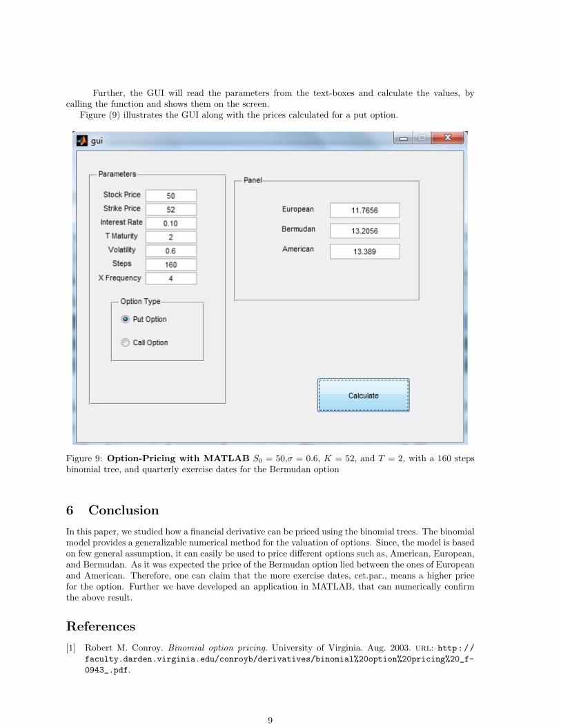
Further, the GUI will read the parameters from the text-boxes and calculate the values, bycalling the function and shows them on the screen.

Figure (9) illustrates the GUI along with the prices calculated for a put option.

Figure 9: Option-Pricing with MATLAB S0 = 50,σ = 0.6, K = 52, and T = 2, with a 160 stepsbinomial tree, and quarterly exercise dates for the Bermudan option

6 Conclusion

In this paper, we studied how a financial derivative can be priced using the binomial trees. The binomialmodel provides a generalizable numerical method for the valuation of options. Since, the model is basedon few general assumption, it can easily be used to price different options such as, American, European,and Bermudan. As it was expected the price of the Bermudan option lied between the ones of Europeanand American. Therefore, one can claim that the more exercise dates, cet.par., means a higher pricefor the option. Further we have developed an application in MATLAB, that can numerically confirmthe above result.

References

[1] Robert M. Conroy. Binomial option pricing. University of Virginia. Aug. 2003. url: http://

faculty.darden.virginia.edu/conroyb/derivatives/binomial%20option%20pricing%20_f-

0943_.pdf.

9

[2] John C. Cox, Stephen A. Ross, and Mark Rubinstein. “Option pricing: A simplified approach”.In: Journal of Financial Economics 7.3 (1979), pp. 229–263. issn: 0304-405X. doi: 10.1016/

0304- 405X(79)90015- 1. url: http://www.sciencedirect.com/science/article/pii/

0304405X79900151.

[3] John Hull. “Options, futures, and other derivatives”. In: Options, futures, and other derivatives.2009.

[4] Masaaki Kijima. Stochastic Processes with Applications to Finance. Chapman and Hall/CRC,2002. isbn: 1584882247. url: http://www.amazon.com/Stochastic-Processes-Applications-Finance - Masaaki / dp / 1584882247 % 3FSubscriptionId % 3D0JYN1NVW651KCA56C102 % 26tag %

3Dtechkie-20%26linkCode%3Dxm2%26camp%3D2025%26creative%3D165953%26creativeASIN%

3D1584882247.

[5] Martin Schweizer. On Bermudan Options. ETH Zurich. Aug. 2012. url: http://www.math.ethz.ch/~mschweiz/Files/bermuda_final.pdf.

[6] Dennis Wackerly, William Mendenhall, and Richard L. Scheaffer. Mathematical Statistics with Ap-plications. Duxbury Press, 2007. isbn: 0495110817. url: http://www.amazon.com/Mathematical-Statistics-Applications-Dennis-Wackerly/dp/0495110817%3FSubscriptionId%3D0JYN1NVW651KCA56C102%

26tag%3Dtechkie-20%26linkCode%3Dxm2%26camp%3D2025%26creative%3D165953%26creativeASIN%

3D0495110817.

10

A Appendix I: MATLAB Codes

f unc t i on [ euPrice , amPrice , brPr i ce ] =b inCa l cu la to r (S ,K, r , sigma ,T,N, exerc i s e Frequency , put True )% Course : MMA707 Ana ly t i c a l Finance I%Seminar in Ana ly t i c a l Finance I%Group : J e s s i c a Radeschnic , Hosse in Nohrouzian ,

Amir KazempourEsmati

%%%%%%%%%%%%% binCa l cu la to r%%%%%%%%%%%%%%%%binCa l cu l a to r implements the CRR binomial t r e e to c a l c u l a t e the f a i r p r i c e%% f o r American , European , and Bermudan opt ions . P lease r e f e r to the seminar% repor t f o r the c a l c u l a t i o n d e t a i l s . %%%%%%%%%%%%%%%%%%%%%%%%%%%%%%%%%%%%%%%%%%%% Parameters Guide%%%%%%%%%%%%%%%%%%%%%%%%%%%%%%%%%%%%%%%%%%%% S : Spot pr i ce , e . g . , 50 .% K: S t r i k e pricem , e . g . , 50 .% r : Risk−f r e e i n t e r e s t r a t e e . g . , 0 . 1 f o r 10%.% sigma : V o l a t i l i t y , e . g . , 0 . 3 f o r 30%.% T: Years to maturity , e . g . , 1 f o r 1 year .% N: Number o f s t ep s in the binomial t r e e .% Exerc i se Frequency : Number o f t imes that the Bermudan opt ion can be% e x e r c i s e d in a year , e . g . , 12 f o r the monthly e x e r c i s e .% put True : 1 f o r put option , 0 f o r a c a l l .%%%%%%%%%%%%%%%%%%%%%%%%%%%%%%%%%%%%%%%%%%%%%%%%%%%%%%%%%%%%%%%%%%%%%%%Author : Amir Kazempour , akr10001@student .mdh. se%%%%%%%%%%%%%%%%%%%%%%%%%%%%%%%%%%%%%%%%%%%%%%%%%%%%%%%%%%%%%%%%%%%%%%%%%%%%%%%

dt= T/N;d = exp(−sigma∗ s q r t ( dt ) ) ; u = exp ( sigma∗ s q r t ( dt ) ) ;p = ( exp ( r ∗dt)−d )/( u−d ) ;d i s count Facto r = exp(−r ∗dt ) ;s tep Length = T/N;e x e r c i s e T r u e= ze ro s (1 ,N) ; %This i s used l a t e r ,%to check i f the e x e r c i s e i s p o s s i b l e at a c e r t a i n node ( in Bermudan t r e e )mCoeff = N / (T∗ exe r c i s e Frequency ) ;

f o r i = mCoeff : mCoeff : Ne x e r c i s e T r u e ( i ) = 1 ;

end

%Creat ing the binomial t r e e from the l a s t node to the f i r s t nodef o r j = N: −1:1

f o r i = j +1: −1 : 1binTree ( i , j ) = S ∗ (u ˆ ( j −2∗( i −1) ) ) ;

endend

%binTreeEE c a l c u l a t e s the payof f , tak ing in to c o n s i d e r a t i o n% only the spot p r i c e s at each node .i f put True

f o r j = N: −1:1f o r i = j +1: −1 : 1

binTreeEE ( i , j ) = max(0 ,K− binTree ( i , j , 1 ) ) ;end

11

ende l s e

f o r j = N: −1:1f o r i = j +1: −1 : 1

binTreeEE ( i , j ) = max(0 , binTree ( i , j ,1)− K ) ;end

endend

%binTreeNE g i v e s the pay−o f f s in case that the opt ion can not be e x e r c i s e d%u n t i l the l a s t node .binTreeNE ( : ,N) = binTreeEE ( : ,N) ;f o r j = N−1: −1:1

f o r i = j +1: −1 : 1binTreeNE ( i , j ) = d i s count Facto r ∗ ( binTreeNE ( i , j +1)∗p +

binTreeNE ( i +1, j +1)∗(1−p) ) ;end

end

binTreeAm ( : ,N) = binTreeEE ( : ,N) ;%Code f o r the American t r e ef o r j = N−1: −1:1

f o r i = j +1: −1 : 1binTreeAm ( i , j ) = max ( binTreeEE ( i , j ) ,

d i s count Facto r ∗ ( binTreeAm ( i , j +1)∗p + binTreeAm ( i +1, j +1)∗(1−p ) ) ) ;end

end

%Code f o r the Bermudan option ,binTreeBr ( : ,N) = binTreeEE ( : ,N) ;f o r j = N−1: −1:1

f o r i = j +1: −1 : 1i f e x e r c i s e T r u e ( j )

binTreeBr ( i , j ) = max ( binTreeEE ( i , j ) ,d i s count Facto r ∗ ( binTreeBr ( i , j +1)∗p + binTreeBr ( i +1, j +1)∗(1−p ) ) ) ;

e l s ebinTreeBr ( i , j ) = d i s count Facto r ∗( binTreeBr ( i , j +1)∗p + binTreeBr ( i +1, j +1)∗(1−p ) ) ;

endend

end

%Options p r i c e s are s to r ed in the c e l l ( 4 , 1 ) o f the r e s p e c t i v e t r e e .euPr ice = d i s count Facto r ∗ ( binTreeNE (1 ,1 )∗p + binTreeNE (2 ,1)∗(1−p) ) ;

amPrice = d i s count Facto r ∗ ( binTreeAm (1 ,1 )∗p + binTreeAm (2 ,1)∗(1−p) ) ;

b rPr i ce = d i s count Facto r ∗ ( binTreeBr (1 ,1 )∗p + binTreeBr (2 ,1)∗(1−p) ) ;%Exporting a l l the p r i c e s to the Pr i c e s vec to r to be used f o r i l l u s t r a t i o n .% P r i c e s = [ binTreeNE ( 4 , 1 ) ; binTreeBr ( 4 , 1 ) ; binTreeAm ( 4 , 1 ) ] ;% bar3 ( Pr i c e s ) ;end

12