Berkeley: Sept 15, 1999 1 Physical Design Challenges of Reconfigurable Computing Systems Majid...
48
Berkeley: Sept 1 5, 1999 1 Physical Design Challenges of Reconfigurable Computing Systems Majid Sarrafzadeh NuCAD Department of ECE Northwestern University Ryan Kastner, Todd Haverkos, Kia Bazargan, Seda Ogrenci, Eli Bozorgzadeh, Candice McGrew Sponsored: DARPA, Motorola, AT&T, NSF
-
date post
21-Dec-2015 -
Category
Documents
-
view
214 -
download
1
Transcript of Berkeley: Sept 15, 1999 1 Physical Design Challenges of Reconfigurable Computing Systems Majid...

Berkeley: Sept 15, 1999 1
Physical Design Challenges of Reconfigurable Computing Systems
Majid SarrafzadehNuCAD
Department of ECENorthwestern University
Ryan Kastner, Todd Haverkos, Kia Bazargan, Seda Ogrenci, Eli Bozorgzadeh, Candice McGrew
Sponsored: DARPA, Motorola, AT&T, NSF

Berkeley: Sept 15, 1999 2
Faculty Position
• In VLSI Design & CAD (1-2 openings)
• VLSI Design & CAD: One of the six focused research areas in the department
• Assistant/Associate/Full Professor– (Northwestern rank: top 10; – ECE: top 20 (top 10 in 5 years)
• Contact: [email protected]

Berkeley: Sept 15, 1999 3
Field Programmable Gate Array: FPGA

Berkeley: Sept 15, 1999 4
FPGA(Xilinx)

Berkeley: Sept 15, 1999 5
Degraded Image Restored Image
Berkeley: Sept 15, 1999 6
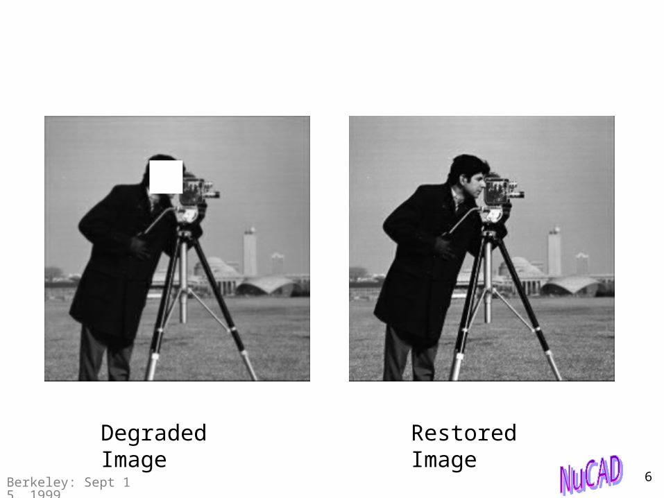
Degraded Image Restored Image

Berkeley: Sept 15, 1999 7
Image stored in on-chip memory
Circuit to process the image
residing on the rest of the chipFPGA chip On-board memory,
where the image is stored
FPGA chip
Host processor
( image is stored here)
System A System B System C

Berkeley: Sept 15, 1999 8
CPU
Data Memory
Control
Data
Data Data
Instruction Memory (Program)
RFUOPs CPU instructions
The Architecture of a Reconfigurable System
RFU

Berkeley: Sept 15, 1999 9
RFU
Programmable logic
Programmable connections
Field Programmable Gate Array: FPGA• SRAM cells used in configuration
– Reconfigurable (runtime)– Static vs. dynamic configuration
• Hardware functions implemented as rectangular areas on the FPGA
SRAM cells

Berkeley: Sept 15, 1999 10
System Components
Configuration Memory
Config. Bits RFUOPs
RFU Manager
PlacementEngine
CacheManager
Prefetch/BranchPrediction Unit
Control
Program Manager
InstructionMem. (Prog.)
CPU instructions
Data
CPU
RFU
Data Memory
Data
Data

Berkeley: Sept 15, 1999 11
System Behavior
• Two kind of instructions– CPU instructions => always run on CPU
• Assume known runtime
– RFUOPs, might be performed on CPU if not enough room on RFU• Assume known runtime and reconfiguration time
• Runtime profiles and RFU status are used to decide between CPU and RFU

Berkeley: Sept 15, 1999 12
PD Challenges• Problem: Given RFUOPs to be performed on RFU and
DFG constraints, schedule them in time assign them physical location.
• Must be very fast: (mtools achieve 1000 cells per minute). Existing tools/techniques are very slow. Quality is less important.
• New PD algorithm/paradigms are needed.
• In this presentation: – placement, – routing, – an application on reconfigurable systems.

Berkeley: Sept 15, 1999 13
Firm Macros• Not hard (too rigid), not soft (takes too
much time to utilize the flexibility)
• Each unit is 80%-100% pre-designed: Can “break” the macros in limited ways
• We have defined a network algebra for combining circuits (based on parameterization using VHDL generics): combine a fast and a slow adder in multiple ways

Berkeley: Sept 15, 1999 14
Faculty Position
• In VLSI Design & CAD (1-2 openings)
• VLSI Design & CAD: One of the six focused research areas in the department
• Assistant/Associate/Full Professor– (Northwestern rank: top 10; – ECE: top 20 (top 10 in 5 years)– Contact: [email protected]

Berkeley: Sept 15, 1999 15
Execution of a Sample Program
RFU
t y
x
x = 3*a - b;…
C = RFUOP1(x,5);
y = 4*x - c;
for (i=0;i<3;i++){
x += RFUOP2(y);
++y;
}
z = RFUOP1(x,3);
a = z - y;
b = RFUOP3(a,b);
c = a - b;
…
CodeCode DFGDFG
=> (on CPU)
(on RFU)=>
=>
=>
No room on RFU to run allin parallel ==> run in sequence
=>
=>
(in parallel)=>
=>
=>

Berkeley: Sept 15, 1999 16
Placement
• On-line placement– RFU calls needs to be executed as the program
proceeds
• off-line placement– Have a complete or partial profile of the
operation

Berkeley: Sept 15, 1999 17
Online Placement• When a new RFUOP arrives
– Is there enough space to place the RFUOP?– If yes, Which location is best to place it?
• Decision 1: Managing the empty space– Fast but sub-optimal
• Keep only O(n) empty rectangles– Shorter Seg. (SSEG), Square Empty Rects. (SQR), ...
– Efficient use of RFU real estate• KAMER: Keep all O(n2) maximal empty rectangles
• Decision 2: Packing rule– Best Fit, Bottom Left, First Fit

Berkeley: Sept 15, 1999 18
Keeping All Empty Rectangles
Keeping O(n) Empty Rectangles - SSEG
Cannotfit
this

Berkeley: Sept 15, 1999 19Area( ) < Area( ) Choose A
Heuristics for Choosing an Empty Rectangle
AB
CurrentPlacement New module
to be inserted
+ = ?
BF (Best Fit) FF (First Fit) BL (Bottom Left)
Places the new module in the empty rectangle which causes less wasted space.
Any of A or B could be chosen for placing the new module.
P1
P2Places the new module in rect w/ lower bottom-left corner, breaking the tie by picking leftmost one. y(P2) < y(P1) Choose B

Berkeley: Sept 15, 1999 20
Heuristics for Choosing a Segment
SSEG (Shorter Seg) BER (Balanced Empty Rects) LSQR (Larger Rect Square)
SQR (Square Rects)LER (Large Empty Rects)LSEG (Longer Seg)
S1
S2
Chooses the shorter of the twosegments.
Chooses the longer of the twosegments.
AB
C
D
S1
S2
AB
C
D
A
B
C
D
A
B
C
D
Chooses the segment which creates less area difference.
Chooses the segment which creates the larger rectangle closer to square.
S1 < S2
S1 < S2
Area(B) - Area(A) > Area(D) - Area(C) AspectRatio(B) > AspectRatio(D)
Chooses the segment which creates the larger empty rectangle.
Chooses the segment which creates empty rectangles closer to squares.
Area(B) > Area(D)
Max{AR(A),AR(B)} < Max{AR(C),AR(D)}AR = AspectRatio

Berkeley: Sept 15, 1999 21
Online Placement Results
Bin-Pack
Data set KAMER SSEG BER LSQR LSEG LER SQR
ra2048 79.25 74.26 61.52 70.36 52.83 73.87 70.36ra4096 84.59 79.1 66.84 74.39 58.37 79.49 74.73ra8192 79.71 73.39 63.23 69.87 55.87 74.88 68.11
FF
ra16384 81.35 75.08 63.59 70.42 55.73 76.13 69.38 Avg(FF) 81.23 75.46 63.80 71.26 55.70 76.09 70.65
ra2048 82.52 77.49 67.18 75.05 58.93 76.46 74.66ra4096 87.06 81.76 73.22 80.32 64.57 81.66 79.78ra8192 82.28 77.57 67.85 73.91 59.04 76.12 73.77
BF
ra16384 84.04 78.81 68.5 75.36 60.92 78.25 75.44 Avg(BF) 83.97 78.91 69.19 76.16 60.86 78.12 75.91
ra2048 81.84 76.22 61.72 73.29 55.57 76.07 71.83ra4096 86.18 81.93 70.29 78.56 62.33 81.42 78.54ra8192 81.17 75.71 65.04 72.9 59.71 76.54 72.18
BL
ra16384 83.46 77.39 64.97 74.53 58.23 78.29 73.25 Avg(BL) 83.16 77.81 65.50 74.82 58.96 78.08 73.95
Table 1. Percentage of accepted modules using different bin-packing and empty space partitioning rules

Berkeley: Sept 15, 1999 22
Online Placement Results
Penalties for different partitioning heuristics when BF is used
0.0E+00
2.0E+07
4.0E+07
6.0E+07
8.0E+07
1.0E+08
1.2E+08
1.4E+08
1.6E+08
1.8E+08
KAMER SSEG BER LSQR LSEG LER SQRPartitioning heuristic
Pen
alty
A2048 A4096 A8192 A16384
Volume that does
not fitBEST

Berkeley: Sept 15, 1999 23
Online Placement Results (cont.)
Running Time Comparison(Time to place "A16384" file)
35.77 34.27 34.74
2.23 2.12 2.24
0
5
10
15
20
25
30
35
40
KAMER SSEG
Tim
e (s
ec.)
BF
FF
BL

Berkeley: Sept 15, 1999 24
ty
x
Off-line placement: 3-D Floorplanning
RFU
DFGDFG ScheduleSchedule
RFU CPU
RFU area
time

Berkeley: Sept 15, 1999 25
ty
x
3-D Floorplanning
RFU
By deleting this RFUOP(CPU performs theoperation)...
DFGDFG ScheduleSchedule
RFU CPU

Berkeley: Sept 15, 1999 26
ty
x
3-D Floorplanning
RFU
DFGDFG ScheduleSchedule
RFU CPU

Berkeley: Sept 15, 1999 27
Our 3-D Floorplanner: No change in the schedule
• Pure annealing– Move set
• Move operation from CPU set to RFU set
• Move operation from RFU set to CPU set
• Displace an already placed RFUOP on the RFU
– Cost function: Volume– Very poor results
• Start with an ASAP schedule, use on-line to get an initial solution, then low-temperature annealing

Berkeley: Sept 15, 1999 28
OfflinePenalty
OnlinePenalty
Ratio
147287 213153 69.10%253566 307879 82.36%464049 508923 91.18%539435 612623 88.05%
Algorithm DatasetT50T100S100S200
LTSAX=100%
A1024 427761 456627 93.68%
T50T100S100S200
LTSAX=20%
A1024
148975 213153 69.89%225603 307879 73.28%287153 508923 56.42%359980 612623 58.76%213036 456627 46.65%
Offline Placement Results
Place X% of the largest-volume modules using on-line placement

Berkeley: Sept 15, 1999 29
Flexibility of the Modules• Library of modules have different
implementations for each RFUOP– Experimental results with our online algorithms
show about 60% reduction in penalty.
• 3-4 Implementations are enough

Berkeley: Sept 15, 1999 30
Faster Routing: mostly offline
Technology-Mapped netlist
ArchitectureDescription File
VPR
Place Circuit or Read in Existing Placement
Perform either Global or Combined Global/Detailed Routing
Placement and Routing Output Files
VP
RC
AD
flo
w

Berkeley: Sept 15, 1999 31
Routing Algorithm (VPR)
Call the VPR’s Router by an arbitrary channel width • Based on PathFinder negotiated congestion algorithm
Step1: Each net routed by the shortest path
which can be found. (Regardless of any overuse of wiring segments)
Step2: Sequentially ripping-up and re-routing
every net in the circuit (by the lowest cost path found)

Berkeley: Sept 15, 1999 32
Fast Pattern Routing
• Maze-based routing algorithm has a good performance but it’s very slow.
So,• Speed-up the router by partially using pattern
routing
if an arbitrary net picked and routed differently, it would not change the result effectively.

Berkeley: Sept 15, 1999 33
Independent subset of nets
Two geometrical independent sets of nets
- Class 1
- Class 2

Berkeley: Sept 15, 1999 34
Routing Patterns
2 terminal net patterns Multi terminal net patterns (MST & RSTs)
Cos
t = L
+ c
onst
/ F
lexi
bili t
y

Berkeley: Sept 15, 1999 35
Implementation of Algorithm• First choose the 2 terminal nets to route - More than 50% of the nets are 2 terminal nets.
- In order to get the maximum independent sets, sort the two terminal nets in terms of their bounding boxes.
- Classify the 2 terminal nets in geometrical independent classes
- Route the classes, sequentially by pattern routing.
• Next choose the multi terminal nets ( low fan-out) - Route them in their corresponding RST patterns
• Finally, let the rest of the nets be routed by traditional router

Berkeley: Sept 15, 1999 36
Experimental Results
Router VPR PATTERN ROUTER
MCNCbenchmark
channelwidth
WL run time channel width
WL run time speed- up%
alu4 10 18601 334.49 10 19188 273.87 23%apex2 10 28410 830.32 11 29056 459.8 80%apex4 11 20503 443.15 12 20137 424.6 4.4%ex5p 12 17585 459.68 13 18020 357.65 28.5%frisc 11 49799 1920 11 50919 1870 2.7%diffeq 7 13796 155.45 8 13684 102.36 51.8%dsip 7 13128 113.19 7 13363 49.24 130%misex3 10 19557 345.59 10 20184 194.7 77.5%pdc 15 92249 6700 17 90988 2430 175%s298 7 19018 207.710 8 18794 74.69 178%s3841 7 55885 1110 8 55573 332.6 234%s38584.1 8 51658 1110 8 52610 603.74 84%seq 10 26130 939.84 11 26694 437.84 114.5%spla 12 59290 4030 12 60874 2350 71.5%tseng 6 8531 96.45 6 8780 39.63 143.4%des 8 20305 479.56 10 20439 311.62 54%ex1010 10 63699 2400 12 62662 914.67 162.4%bigkey 7 15808 135.94 7 16158 113.64 19.6%
average 9.3 30310.11 1122.57 10 33229 630 82.46%

Berkeley: Sept 15, 1999 37
Faculty Position
• In VLSI Design & CAD (1-2 openings)
• VLSI Design & CAD: One of the six focused research areas in the department
• Assistant/Associate/Full Professor– (Northwestern rank: top 10; – ECE: top 20 (top 10 in 5 years)– Contact: [email protected]

Berkeley: Sept 15, 1999 38
r0
r1
Image Restoration
The value of the center pixel in the next iteration:
xk+1 = *y + xk - * (d**xk)
r1r1
r1 r1 r1
r1
y: the pixel value from the original degraded image
xk: the pixel value from the previous iteration
d**xk denotes the weighted sumr1* (eight neighbor pixels) + r0 * center
pixel

Berkeley: Sept 15, 1999 39
Incentive : Processing of large sized images
using FPGA’s with limited resources
1. Segmentation of the image into smaller
sized images suitable for the FPGA
Segments of size m x n are surrounded
by an overlap of o.
m
o
n

Berkeley: Sept 15, 1999 40
. Pixels of individual segments are restored in parallel by hardware
. Restored segments are written back after the overlap is discarded
MEMORY
m
o
nRFU

Berkeley: Sept 15, 1999 41
How bad is the segmentation?• Theorem: The error introduces is about (w)**O example: (1/16) ** 2 = (1/264)
• Proof: By induction
m
o
n

Berkeley: Sept 15, 1999 42
Comparison of Image Qualities
1.6
1.8
2
2.2
2.4
2.6
2.8
3
3.2
8 16 32 64 128
Segment Sizes
ISN
R (d
B)
Cameraman(segmented)
Cameraman(sequential)
Moon (sequential)
Moon (segmented)

Berkeley: Sept 15, 1999 43
Degraded Image Restored Image

Berkeley: Sept 15, 1999 44
Degraded Image Restored Image

Berkeley: Sept 15, 1999 45
Image stored in on-chip memory
Circuit to process the image
residing on the rest of the chipFPGA chip On-board memory,
where the image is stored
FPGA chip
Host processor
( image is stored here)
System A System B System C

Berkeley: Sept 15, 1999 46
Image Software RunningTime (sec)
Running Timefor System A
(msec)
Running Time for System C
(msec)cameraman 4.772 9.157 91.960
moon 2.812 5.725 54.494
circle 2.987 4.254 42.722
animals 6.761 8.826 88.628
fish 7.029 14.026 140.850
barbara 21.741 36.630 367.840
yacht 12.367 34.079 342.227
soccer 12.360 34.079 342.227
announcer 13.462 34.079 342.227
bluegirl 10.158 34.079 342.227
cablecar 12.354 34.079 342.227
cornfield 13.458 34.079 342.227
Running Times of the Application on Software and on Different Systems
(ignoring reconfiguration)

Berkeley: Sept 15, 1999 47
Conclusions• Need radical departure (new algorithm, etc)
from traditional PD algorithms.
• Fast (and lower quality) place & route tools
• Do as much as possible (building complex libraries, hierarchical routing, …) before compilation
• All of the above (and more) needed to make reconfigurable computing a reality.

Berkeley: Sept 15, 1999 48
Faculty Position
• In VLSI Design & CAD (1-2 openings)
• VLSI Design & CAD: One of the six focused research areas in the department
• Assistant/Associate/Full Professor– (Northwestern rank: top 10; – ECE: top 20 (top 10 in 5 years)
• Contact: [email protected]