Bentley MicroStation Workshop 2017 FLUG Fall Training...
25
Bentley MicroStation Workshop 2017 FLUG Fall Training Event F-2E - Modeling Designing 2D/3D Curves in MicroStation CONNECT Edition Bentley Systems, Incorporated 685 Stockton Drive Exton, PA 19341 www.bentley.com
-
Upload
truongngoc -
Category
Documents
-
view
234 -
download
3
Transcript of Bentley MicroStation Workshop 2017 FLUG Fall Training...

Bentley MicroStation Workshop
2017 FLUG Fall Training Event
F-2E - Modeling Designing 2D/3D Curves in MicroStation CONNECT Edition
Bentley Systems, Incorporated 685 Stockton Drive Exton, PA 19341 www.bentley.com
Copyright © Bentley Systems, Incorporated DO NOT DISTRIBUTE – Printing for student use is permitted 1
Practice Workbook This workbook is designed for use in Live instructor-led training and for OnDemand self-study. The explanations
and demonstrations are provided by the instructor in the classroom, or in the OnDemand eLectures of this course
available on the Bentley LEARNserver (learn.bentley.com).
This practice workbook is formatted for on-screen viewing using a PDF reader. It is also available as a PDF
document in the dataset for this course.
Modeling and Designing 2D/3D Curves in
MicroStation CONNECT Edition
This workbook contains exercises to help you learn how to create, evaluate, and modify B-spline curves and their
special cases like parabola to meet specific engineering design goals.
TRNC02417-1/0001
Copyright © Bentley Systems, Incorporated DO NOT DISTRIBUTE – Printing for student use is permitted 2
Modeling and Designing 2D/3D Curves
This course covers -
Helices – Conical and Cylindrical Hands on Exercise
Spirals Hands on Exercise
Logarithmic Spiral – Approximation with Lines Hands on Exercise
Archimedes Spirals – Approximation with Arcs Hands on Exercise
Creation of a Curve from its Equation/ Formula Hands on Exercise
Related Math concepts (offer more powerful and flexible usage of the tools, but could be skipped)
How to use this course?
This course can be undertaken to accomplish two goals.
1. Learn the Workflow – A procedural track, where tools and steps are learned using hands on exercises. With intermediate MicroStation
skills, this track can be completed in about 2 hours.
2. Understand the Formulation – Mathematical concepts and calculations needed when the data or goal does not directly relate to
MicroStation tool settings. E.g. slope of a helical ramp of a parking structure is an important design aspect, but it cannot be directly specified.
So knowing the formulae to convert it into pitch and radius (available in the Tool Setting), helps plot desired helix. Concepts are presented in
an intuitive form rather than abstract rigor and based on familiarity, this part would take an additional hour.
How to navigate?
A purely procedural track can be followed by skipping the mathematical formulations marked [Optional] or by clicking the skip links. Following the
entire course sequentially would cover the procedural track along with the theoretical background.
Copyright © Bentley Systems, Incorporated DO NOT DISTRIBUTE – Printing for student use is permitted 3
Helix Back to Index
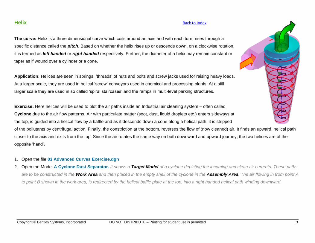
The curve: Helix is a three dimensional curve which coils around an axis and with each turn, rises through a
specific distance called the pitch. Based on whether the helix rises up or descends down, on a clockwise rotation,
it is termed as left handed or right handed respectively. Further, the diameter of a helix may remain constant or
taper as if wound over a cylinder or a cone.
Application: Helices are seen in springs, ‘threads’ of nuts and bolts and screw jacks used for raising heavy loads.
At a larger scale, they are used in helical ‘screw’ conveyors used in chemical and processing plants. At a still
larger scale they are used in so called ‘spiral staircases’ and the ramps in multi-level parking structures.
Exercise: Here helices will be used to plot the air paths inside an Industrial air cleaning system – often called
Cyclone due to the air flow patterns. Air with particulate matter (soot, dust, liquid droplets etc.) enters sideways at
the top, is guided into a helical flow by a baffle and as it descends down a cone along a helical path, it is stripped
of the pollutants by centrifugal action. Finally, the constriction at the bottom, reverses the flow of (now cleaned) air. It finds an upward, helical path
closer to the axis and exits from the top. Since the air rotates the same way on both downward and upward journey, the two helices are of the
opposite ‘hand’.
1. Open the file 03 Advanced Curves Exercise.dgn
2. Open the Model A Cyclone Dust Separator. It shows a Target Model of a cyclone depicting the incoming and clean air currents. These paths
are to be constructed in the Work Area and then placed in the empty shell of the cyclone in the Assembly Area. The air flowing in from point A
to point B shown in the work area, is redirected by the helical baffle plate at the top, into a right handed helical path winding downward.
Copyright © Bentley Systems, Incorporated DO NOT DISTRIBUTE – Printing for student use is permitted 4
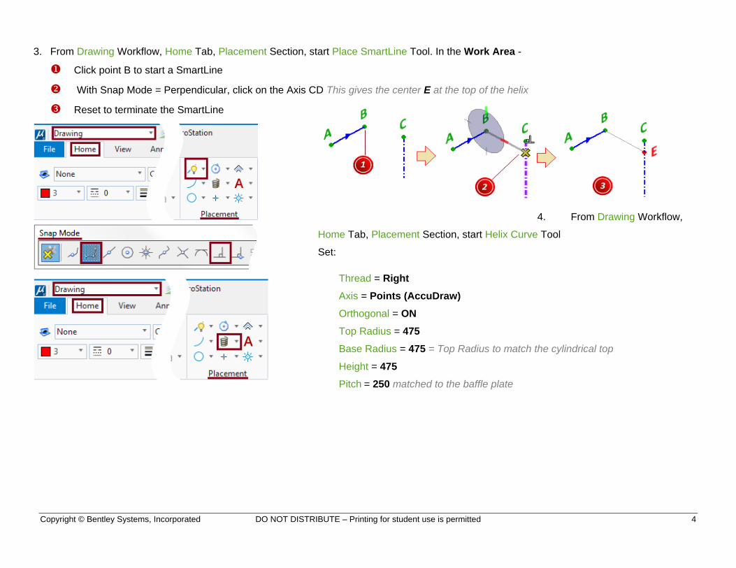
3. From Drawing Workflow, Home Tab, Placement Section, start Place SmartLine Tool. In the Work Area -
Click point B to start a SmartLine
With Snap Mode = Perpendicular, click on the Axis CD This gives the center E at the top of the helix
Reset to terminate the SmartLine
4. From Drawing Workflow,
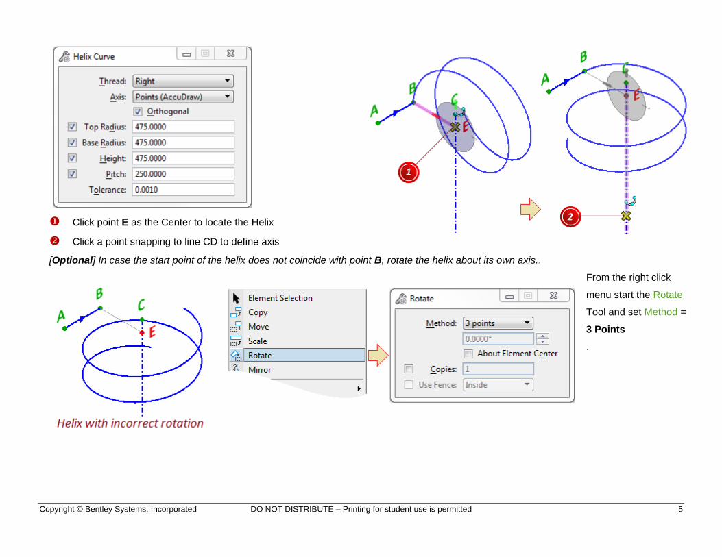
Home Tab, Placement Section, start Helix Curve Tool
Set:
Thread = Right
Axis = Points (AccuDraw)
Orthogonal = ON
Top Radius = 475
Base Radius = 475 = Top Radius to match the cylindrical top
Height = 475
Pitch = 250 matched to the baffle plate
Copyright © Bentley Systems, Incorporated DO NOT DISTRIBUTE – Printing for student use is permitted 5
Click point E as the Center to locate the Helix
Click a point snapping to line CD to define axis
[Optional] In case the start point of the helix does not coincide with point B, rotate the helix about its own axis..
From the right click
menu start the Rotate
Tool and set Method =
3 Points
.
Copyright © Bentley Systems, Incorporated DO NOT DISTRIBUTE – Printing for student use is permitted 6
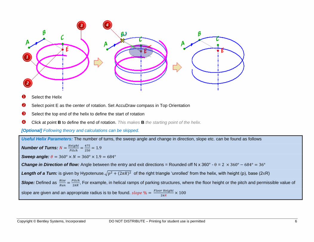
Select the Helix
Select point E as the center of rotation. Set AccuDraw compass in Top Orientation
Select the top end of the helix to define the start of rotation
Click at point B to define the end of rotation. This makes B the starting point of the helix.
[Optional] Following theory and calculations can be skipped.
Useful Helix Parameters: The number of turns, the sweep angle and change in direction, slope etc. can be found as follows
Number of Turns: 𝑁 =𝐻𝑒𝑖𝑔ℎ𝑡
𝑃𝑖𝑡𝑐ℎ=
475
250= 1.9
Sweep angle: 𝜃 = 360° × 𝑁 = 360° × 1.9 = 684°
Change in Direction of flow: Angle between the entry and exit directions = Rounded off N x 360° - = 2 × 360° − 684° = 36°
Length of a Turn: is given by Hypotenuse.√𝑝2 + (2𝜋𝑅)2 of the right triangle ‘unrolled’ from the helix, with height (p), base (2R)
Slope: Defined as 𝑅𝑖𝑠𝑒
𝑅𝑢𝑛=
𝑃𝑖𝑡𝑐ℎ
2𝜋𝑅, For example, in helical ramps of parking structures, where the floor height or the pitch and permissible value of
slope are given and an appropriate radius is to be found. 𝑠𝑙𝑜𝑝𝑒 % = 𝐹𝑙𝑜𝑜𝑟 𝐻𝑒𝑖𝑔ℎ𝑡
2𝜋𝑅× 100
Copyright © Bentley Systems, Incorporated DO NOT DISTRIBUTE – Printing for student use is permitted 7
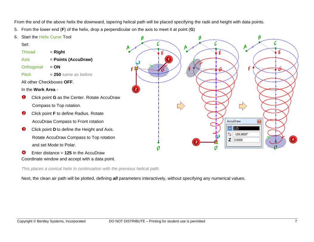
From the end of the above helix the downward, tapering helical path will be placed specifying the radii and height with data points.
5. From the lower end (F) of the helix, drop a perpendicular on the axis to meet it at point (G)
6. Start the Helix Curve Tool
Set:
Thread = Right
Axis = Points (AccuDraw)
Orthogonal = ON
Pitch = 250 same as before
All other Checkboxes OFF.
In the Work Area -
Click point G as the Center. Rotate AccuDraw
Compass to Top rotation.
Click point F to define Radius. Rotate
AccuDraw Compass to Front rotation
Click point D to define the Height and Axis.
Rotate AccuDraw Compass to Top rotation
and set Mode to Polar.
Enter distance = 125 in the AccuDraw
Coordinate window and accept with a data point.
This places a conical helix in continuation with the previous helical path.
Next, the clean air path will be plotted, defining all parameters interactively, without specifying any numerical values.
Copyright © Bentley Systems, Incorporated DO NOT DISTRIBUTE – Printing for student use is permitted 8
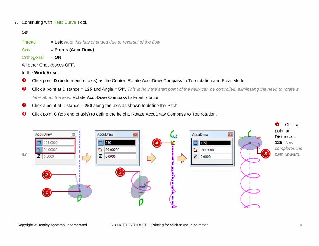
7. Continuing with Helix Curve Tool,
Set
Thread = Left Note this has changed due to reversal of the flow
Axis = Points (AccuDraw)
Orthogonal = ON
All other Checkboxes OFF.
In the Work Area -
Click point D (bottom end of axis) as the Center. Rotate AccuDraw Compass to Top rotation and Polar Mode.
Click a point at Distance = 125 and Angle = 54°. This is how the start point of the helix can be controlled, eliminating the need to rotate it
later about the axis. Rotate AccuDraw Compass to Front rotation
Click a point at Distance = 250 along the axis as shown to define the Pitch.
Click point C (top end of axis) to define the height. Rotate AccuDraw Compass to Top rotation.
Click a
point at
Distance =
125. This
completes the
air path upward.
Copyright © Bentley Systems, Incorporated DO NOT DISTRIBUTE – Printing for student use is permitted 9
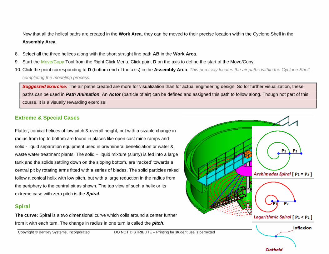
Now that all the helical paths are created in the Work Area, they can be moved to their precise location within the Cyclone Shell in the
Assembly Area.
8. Select all the three helices along with the short straight line path AB in the Work Area.
9. Start the Move/Copy Tool from the Right Click Menu. Click point D on the axis to define the start of the Move/Copy.
10. Click the point corresponding to D (bottom end of the axis) in the Assembly Area. This precisely locates the air paths within the Cyclone Shell,
completing the modeling process.
Suggested Exercise: The air paths created are more for visualization than for actual engineering design. So for further visualization, these
paths can be used in Path Animation. An Actor (particle of air) can be defined and assigned this path to follow along. Though not part of this
course, it is a visually rewarding exercise!
Extreme & Special Cases
Flatter, conical helices of low pitch & overall height, but with a sizable change in
radius from top to bottom are found in places like open cast mine ramps and
solid - liquid separation equipment used in ore/mineral beneficiation or water &
waste water treatment plants. The solid – liquid mixture (slurry) is fed into a large
tank and the solids settling down on the sloping bottom, are ‘racked’ towards a
central pit by rotating arms fitted with a series of blades. The solid particles raked
follow a conical helix with low pitch, but with a large reduction in the radius from
the periphery to the central pit as shown. The top view of such a helix or its
extreme case with zero pitch is the Spiral.
Spiral Back to Index
The curve: Spiral is a two dimensional curve which coils around a center further
from it with each turn. The change in radius in one turn is called the pitch.
Copyright © Bentley Systems, Incorporated DO NOT DISTRIBUTE – Printing for student use is permitted 10
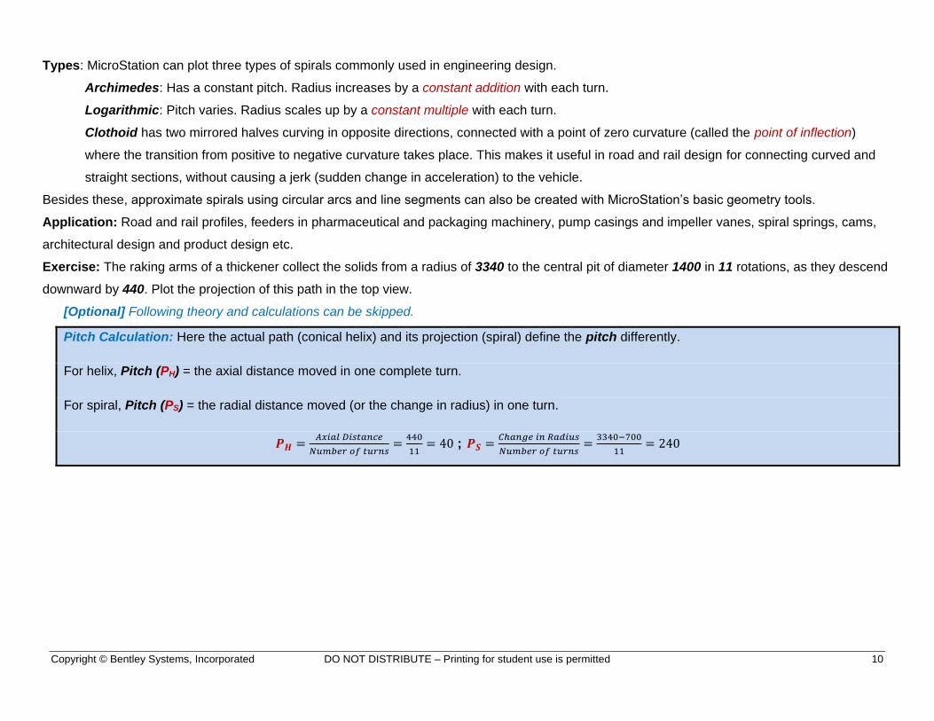
Types: MicroStation can plot three types of spirals commonly used in engineering design.
Archimedes: Has a constant pitch. Radius increases by a constant addition with each turn.
Logarithmic: Pitch varies. Radius scales up by a constant multiple with each turn.
Clothoid has two mirrored halves curving in opposite directions, connected with a point of zero curvature (called the point of inflection)
where the transition from positive to negative curvature takes place. This makes it useful in road and rail design for connecting curved and
straight sections, without causing a jerk (sudden change in acceleration) to the vehicle.
Besides these, approximate spirals using circular arcs and line segments can also be created with MicroStation’s basic geometry tools.
Application: Road and rail profiles, feeders in pharmaceutical and packaging machinery, pump casings and impeller vanes, spiral springs, cams,
architectural design and product design etc.
Exercise: The raking arms of a thickener collect the solids from a radius of 3340 to the central pit of diameter 1400 in 11 rotations, as they descend
downward by 440. Plot the projection of this path in the top view.
[Optional] Following theory and calculations can be skipped.
Pitch Calculation: Here the actual path (conical helix) and its projection (spiral) define the pitch differently.
For helix, Pitch (PH) = the axial distance moved in one complete turn.
For spiral, Pitch (PS) = the radial distance moved (or the change in radius) in one turn.
𝑷𝑯 =𝐴𝑥𝑖𝑎𝑙 𝐷𝑖𝑠𝑡𝑎𝑛𝑐𝑒
𝑁𝑢𝑚𝑏𝑒𝑟 𝑜𝑓 𝑡𝑢𝑟𝑛𝑠=
440
11= 40 ; 𝑷𝑺 =
𝐶ℎ𝑎𝑛𝑔𝑒 𝑖𝑛 𝑅𝑎𝑑𝑖𝑢𝑠
𝑁𝑢𝑚𝑏𝑒𝑟 𝑜𝑓 𝑡𝑢𝑟𝑛𝑠=
3340−700
11= 240
Copyright © Bentley Systems, Incorporated DO NOT DISTRIBUTE – Printing for student use is permitted 11
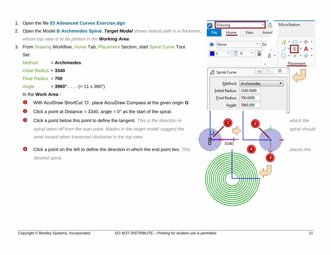
1. Open the file 03 Advanced Curves Exercise.dgn
2. Open the Model B Archimedes Spiral. Target Model shows helical path in a thickener,
whose top view is to be plotted in the Working Area.
3. From Drawing Workflow, Home Tab, Placement Section, start Spiral Curve Tool.
Set
Method = Archimedes
Initial Radius = 3340
Final Radius = 700
Angle = 3960° . . . . (= 11 x 360°)
In the Work Area -
With AcciDraw ShortCut ‘O’, place AccuDraw Compass at the given origin O.
Click a point at Distance = 3340, angle = 0° as the start of the spiral.
Click a point below this point to define the tangent. This is the direction in which the
spiral takes off from the start point. Blades in the target model suggest the spiral should
wind inward when traversed clockwise in the top view.
Click a point on the left to define the direction in which the end point lies. This places the
desired spiral.
Copyright © Bentley Systems, Incorporated DO NOT DISTRIBUTE – Printing for student use is permitted 12
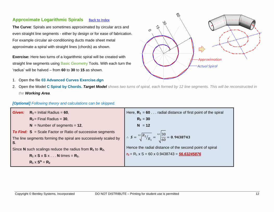
Approximate Logarithmic Spirals Back to Index
The Curve: Spirals are sometimes approximated by circular arcs and
even straight line segments - either by design or for ease of fabrication.
For example circular air-conditioning ducts made sheet metal
approximate a spiral with straight lines (chords) as shown.
Exercise: Here two turns of a logarithmic spiral will be created with
straight line segments using Basic Geometry Tools. With each turn the
‘radius’ will be halved – from 60 to 30 to 15 as shown.
1. Open the file 03 Advanced Curves Exercise.dgn
2. Open the Model C Spiral by Chords. Target Model shows two turns of spiral, each formed by 12 line segments. This will be reconstructed in
the Working Area.
[Optional] Following theory and calculations can be skipped.
Given: R1 = Initial Radius = 60,
R2 = Final Radius = 30,
N = Number of segments = 12,
To Find: S = Scale Factor or Ratio of successive segments
The line segments forming the spiral are successively scaled by S.
Since N such scalings reduce the radius from R1 to R2,
R1 x S x S x . . . N times = R2,
R1 x SN = R2
Here, R1 = 60 . . . radial distance of first point of the spiral
R2 = 30
N = 12
∴ 𝑺 = √𝑅2𝑅1
⁄12
= √30
60
12
= 𝟎. 𝟗𝟒𝟑𝟖𝟕𝟒𝟑
Hence the radial distance of the second point of spiral
r2 = R1 x S = 60 x 0.9438743 = 56.63245876
Copyright © Bentley Systems, Incorporated DO NOT DISTRIBUTE – Printing for student use is permitted 13
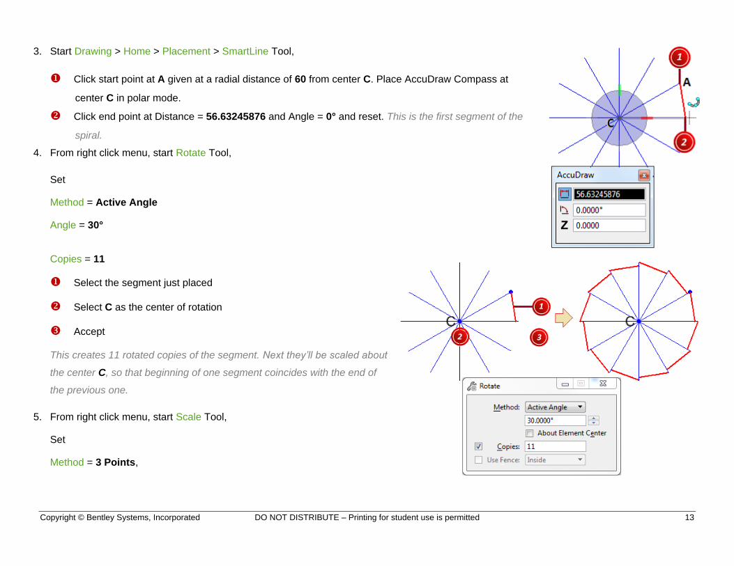
3. Start Drawing > Home > Placement > SmartLine Tool,
Click start point at A given at a radial distance of 60 from center C. Place AccuDraw Compass at
center C in polar mode.
Click end point at Distance = 56.63245876 and Angle = 0° and reset. This is the first segment of the
spiral.
4. From right click menu, start Rotate Tool,
Set
Method = Active Angle
Angle = 30°
Copies = 11
Select the segment just placed
Select C as the center of rotation
Accept
This creates 11 rotated copies of the segment. Next they’ll be scaled about
the center C, so that beginning of one segment coincides with the end of
the previous one.
5. From right click menu, start Scale Tool,
Set
Method = 3 Points,
Copyright © Bentley Systems, Incorporated DO NOT DISTRIBUTE – Printing for student use is permitted 14
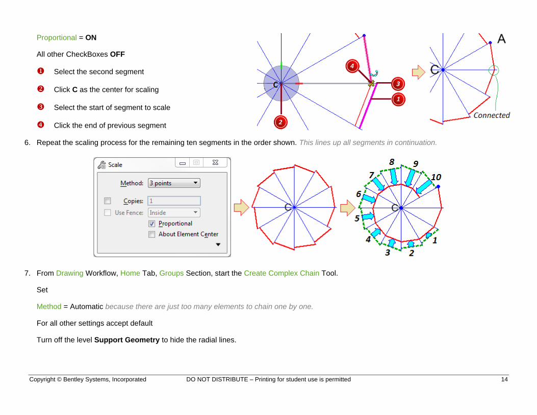
Proportional = ON
All other CheckBoxes OFF
Select the second segment
Click C as the center for scaling
Select the start of segment to scale
Click the end of previous segment
6. Repeat the scaling process for the remaining ten segments in the order shown. This lines up all segments in continuation.
7. From Drawing Workflow, Home Tab, Groups Section, start the Create Complex Chain Tool.
Set
Method = Automatic because there are just too many elements to chain one by one.
For all other settings accept default
Turn off the level Support Geometry to hide the radial lines.
Copyright © Bentley Systems, Incorporated DO NOT DISTRIBUTE – Printing for student use is permitted 15
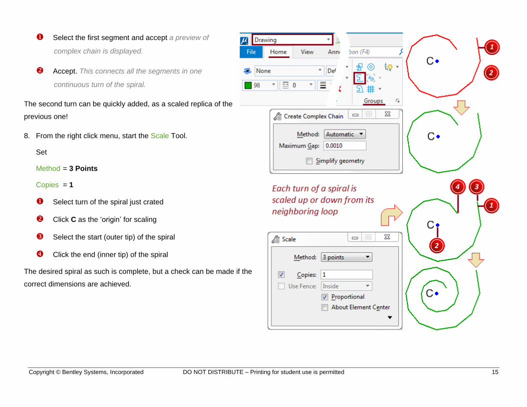
Select the first segment and accept a preview of
complex chain is displayed.
Accept. This connects all the segments in one
continuous turn of the spiral.
The second turn can be quickly added, as a scaled replica of the
previous one!
8. From the right click menu, start the Scale Tool.
Set
Method = 3 Points
Copies = 1
Select turn of the spiral just crated
Click C as the ‘origin’ for scaling
Select the start (outer tip) of the spiral
Click the end (inner tip) of the spiral
The desired spiral as such is complete, but a check can be made if the
correct dimensions are achieved.
Copyright © Bentley Systems, Incorporated DO NOT DISTRIBUTE – Printing for student use is permitted 16
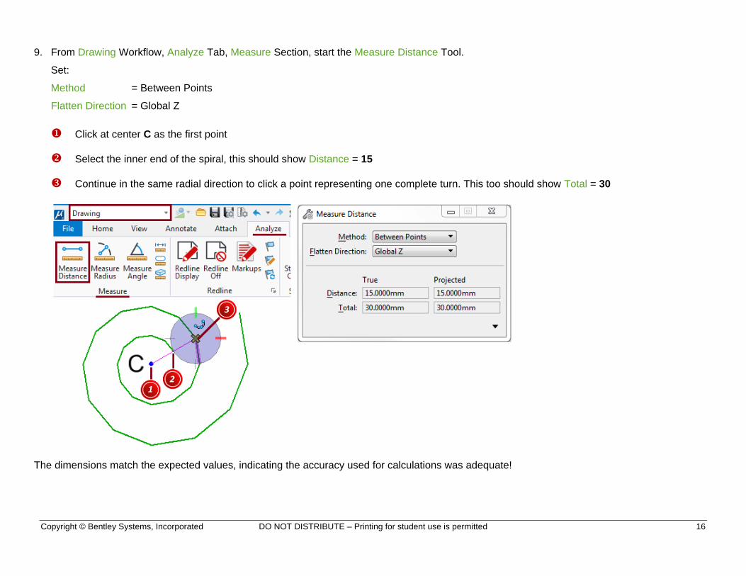
9. From Drawing Workflow, Analyze Tab, Measure Section, start the Measure Distance Tool.
Set:
Method = Between Points
Flatten Direction = Global Z
Click at center C as the first point
Select the inner end of the spiral, this should show Distance = 15
Continue in the same radial direction to click a point representing one complete turn. This too should show Total = 30
The dimensions match the expected values, indicating the accuracy used for calculations was adequate!
Copyright © Bentley Systems, Incorporated DO NOT DISTRIBUTE – Printing for student use is permitted 17
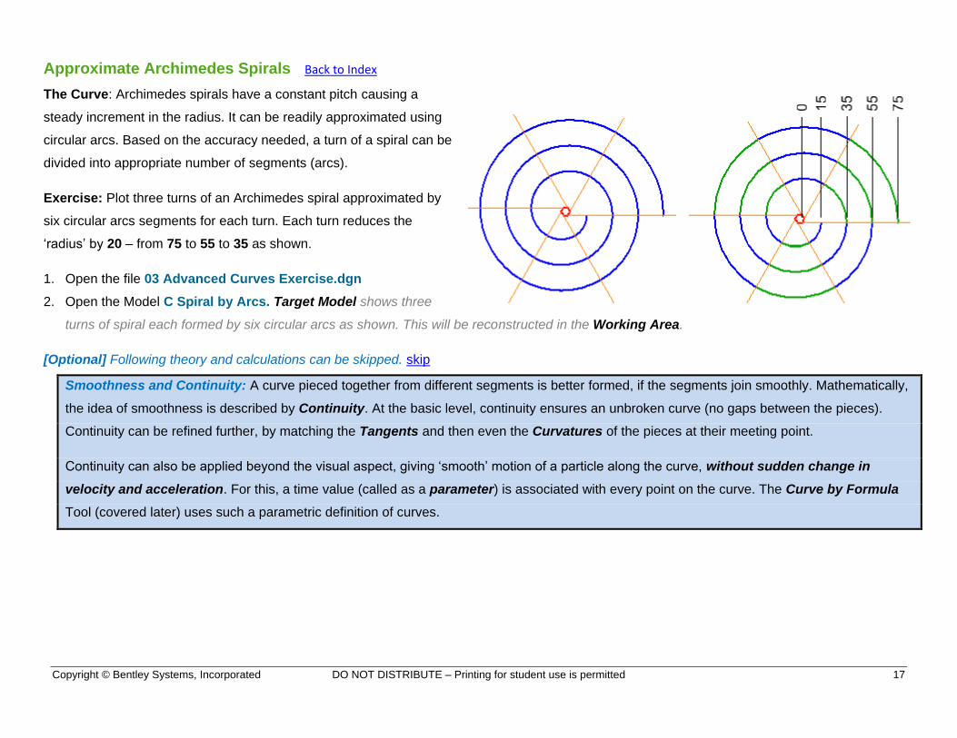
Approximate Archimedes Spirals Back to Index
The Curve: Archimedes spirals have a constant pitch causing a
steady increment in the radius. It can be readily approximated using
circular arcs. Based on the accuracy needed, a turn of a spiral can be
divided into appropriate number of segments (arcs).
Exercise: Plot three turns of an Archimedes spiral approximated by
six circular arcs segments for each turn. Each turn reduces the
‘radius’ by 20 – from 75 to 55 to 35 as shown.
1. Open the file 03 Advanced Curves Exercise.dgn
2. Open the Model C Spiral by Arcs. Target Model shows three
turns of spiral each formed by six circular arcs as shown. This will be reconstructed in the Working Area.
[Optional] Following theory and calculations can be skipped. skip
Smoothness and Continuity: A curve pieced together from different segments is better formed, if the segments join smoothly. Mathematically,
the idea of smoothness is described by Continuity. At the basic level, continuity ensures an unbroken curve (no gaps between the pieces).
Continuity can be refined further, by matching the Tangents and then even the Curvatures of the pieces at their meeting point.
Continuity can also be applied beyond the visual aspect, giving ‘smooth’ motion of a particle along the curve, without sudden change in
velocity and acceleration. For this, a time value (called as a parameter) is associated with every point on the curve. The Curve by Formula
Tool (covered later) uses such a parametric definition of curves.
Copyright © Bentley Systems, Incorporated DO NOT DISTRIBUTE – Printing for student use is permitted 18
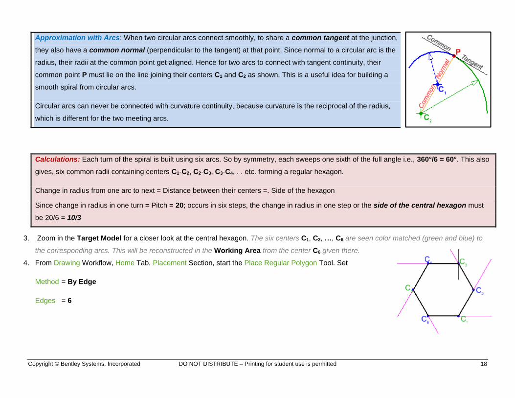
Approximation with Arcs: When two circular arcs connect smoothly, to share a common tangent at the junction,
they also have a common normal (perpendicular to the tangent) at that point. Since normal to a circular arc is the
radius, their radii at the common point get aligned. Hence for two arcs to connect with tangent continuity, their
common point P must lie on the line joining their centers C1 and C2 as shown. This is a useful idea for building a
smooth spiral from circular arcs.
Circular arcs can never be connected with curvature continuity, because curvature is the reciprocal of the radius,
which is different for the two meeting arcs.
Calculations: Each turn of the spiral is built using six arcs. So by symmetry, each sweeps one sixth of the full angle i.e., 360°/6 = 60°. This also
gives, six common radii containing centers C1-C2, C2-C3, C3-C4, . . etc. forming a regular hexagon.
Change in radius from one arc to next = Distance between their centers =. Side of the hexagon
Since change in radius in one turn = Pitch = 20; occurs in six steps, the change in radius in one step or the side of the central hexagon must
be 20/6 = 10/3
3. Zoom in the Target Model for a closer look at the central hexagon. The six centers C1, C2, …, C6 are seen color matched (green and blue) to
the corresponding arcs. This will be reconstructed in the Working Area from the center C6 given there.
4. From Drawing Workflow, Home Tab, Placement Section, start the Place Regular Polygon Tool. Set
Method = By Edge
Edges = 6
Copyright © Bentley Systems, Incorporated DO NOT DISTRIBUTE – Printing for student use is permitted 19
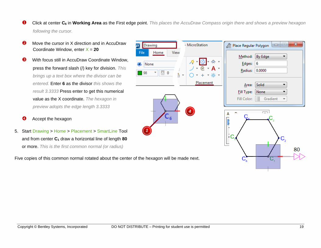
Click at center C6 in Working Area as the First edge point. This places the AccuDraw Compass origin there and shows a preview hexagon
following the cursor.
Move the cursor in X direction and in AccuDraw
Coordinate Window, enter X = 20
With focus still in AccuDraw Coordinate Window,
press the forward slash (/) key for division. This
brings up a text box where the divisor can be
entered. Enter 6 as the divisor this shows the
result 3.3333 Press enter to get this numerical
value as the X coordinate. The hexagon in
preview adopts the edge length 3.3333
Accept the hexagon
5. Start Drawing > Home > Placement > SmartLine Tool
and from center C1 draw a horizontal line of length 80
or more. This is the first common normal (or radius)
Five copies of this common normal rotated about the center of the hexagon will be made next.
Copyright © Bentley Systems, Incorporated DO NOT DISTRIBUTE – Printing for student use is permitted 20
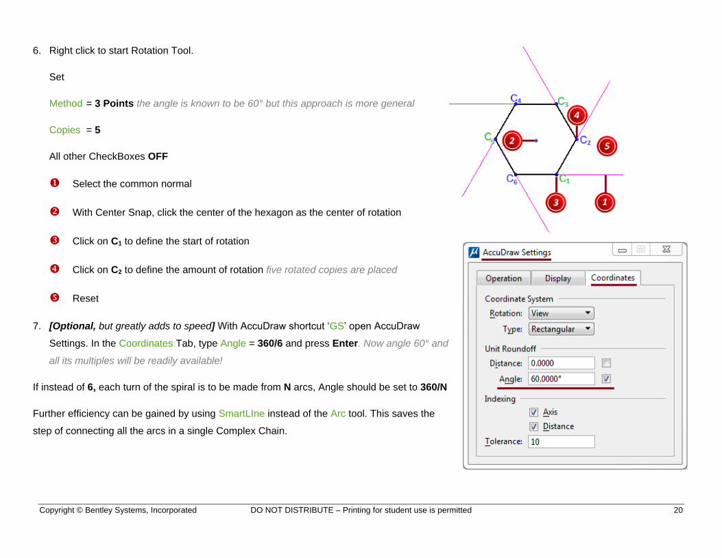
6. Right click to start Rotation Tool.
Set
Method = 3 Points the angle is known to be 60° but this approach is more general
Copies = 5
All other CheckBoxes OFF
Select the common normal
With Center Snap, click the center of the hexagon as the center of rotation
Click on C1 to define the start of rotation
Click on C2 to define the amount of rotation five rotated copies are placed
Reset
7. [Optional, but greatly adds to speed] With AccuDraw shortcut ‘GS’ open AccuDraw
Settings. In the Coordinates Tab, type Angle = 360/6 and press Enter. Now angle 60° and
all its multiples will be readily available!
If instead of 6, each turn of the spiral is to be made from N arcs, Angle should be set to 360/N
Further efficiency can be gained by using SmartLIne instead of the Arc tool. This saves the
step of connecting all the arcs in a single Complex Chain.
Copyright © Bentley Systems, Incorporated DO NOT DISTRIBUTE – Printing for student use is permitted 21
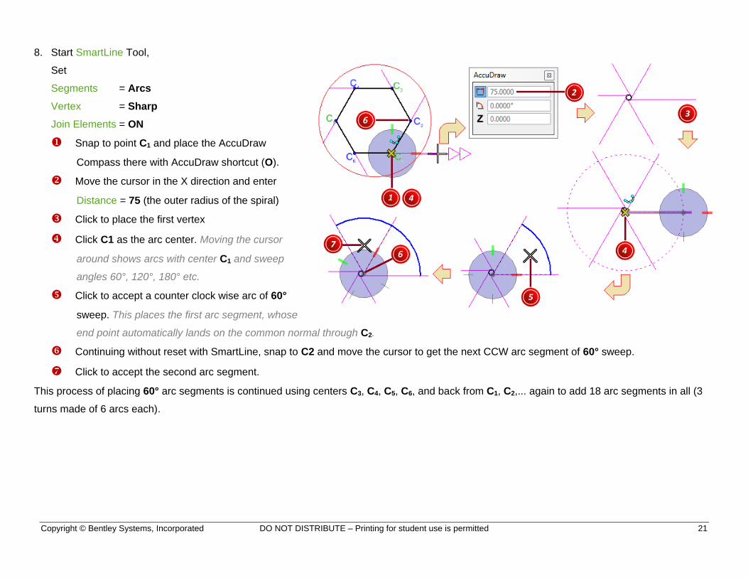
8. Start SmartLine Tool,
Set
Segments = Arcs
Vertex = Sharp
Join Elements = ON
Snap to point C1 and place the AccuDraw
Compass there with AccuDraw shortcut (O).
Move the cursor in the X direction and enter
Distance = 75 (the outer radius of the spiral)
Click to place the first vertex
Click C1 as the arc center. Moving the cursor
around shows arcs with center C1 and sweep
angles 60°, 120°, 180° etc.
Click to accept a counter clock wise arc of 60°
sweep. This places the first arc segment, whose
end point automatically lands on the common normal through C2.
Continuing without reset with SmartLine, snap to C2 and move the cursor to get the next CCW arc segment of 60° sweep.
Click to accept the second arc segment.
This process of placing 60° arc segments is continued using centers C3, C4, C5, C6, and back from C1, C2,... again to add 18 arc segments in all (3
turns made of 6 arcs each).
Copyright © Bentley Systems, Incorporated DO NOT DISTRIBUTE – Printing for student use is permitted 22
Curve by Formula Back to Index
MicroStation’s Curve by Formula Tool can plot virtually any curve (2D or 3D), given in a Parametric form, which expresses the coordinates (x, y,
z) of a point on the curve in terms of a parameter (t). The curve is then plotted as a Bspline.
[Optional] Following theory and calculations can be skipped.
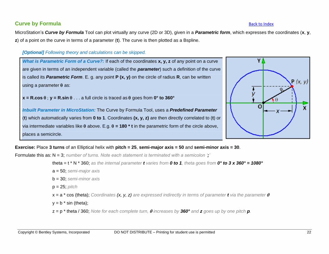
What is Parametric Form of a Curve?: If each of the coordinates x, y, z of any point on a curve
are given in terms of an independent variable (called the parameter) such a definition of the curve
is called its Parametric Form. E. g. any point P (x, y) on the circle of radius R, can be written
using a parameter as:
x = R.cos y = R.sin . . . a full circle is traced as goes from 0° to 360°
Inbuilt Parameter in MicroStation: The Curve by Formula Tool, uses a Predefined Parameter
(t) which automatically varies from 0 to 1. Coordinates (x, y, z) are then directly correlated to (t) or
via intermediate variables like above. E.g. = 180 * t in the parametric form of the circle above,
places a semicircle.
Exercise: Place 3 turns of an Elliptical helix with pitch = 25, semi-major axis = 50 and semi-minor axis = 30.
Formulate this as: N = 3; number of turns. Note each statement is terminated with a semicolon ‘;’
theta = t * N * 360; as the internal parameter t varies from 0 to 1, theta goes from 0° to 3 x 360° = 1080°
a = 50; semi-major axis
b = 30; semi-minor axis
p = 25; pitch
x = a * cos (theta); Coordinates (x, y, z) are expressed indirectly in terms of parameter t via the parameter
y = b * sin (theta);
z = p * theta / 360; Note for each complete turn, increases by 360° and z goes up by one pitch p.
Copyright © Bentley Systems, Incorporated DO NOT DISTRIBUTE – Printing for student use is permitted 23
Note a semicolon (;) at end of each line. Operators (*) & (/) stand for multiplication and division. Trigonometric Functions like Sin and Cos can be
directly used.
1. Open the file 03 Advanced Curves Exercise.dgn
2. Open the Model E Curve by Formula. Target Model shows three turns of an elliptical spiral. This is to be reconstructed in the Working Area.
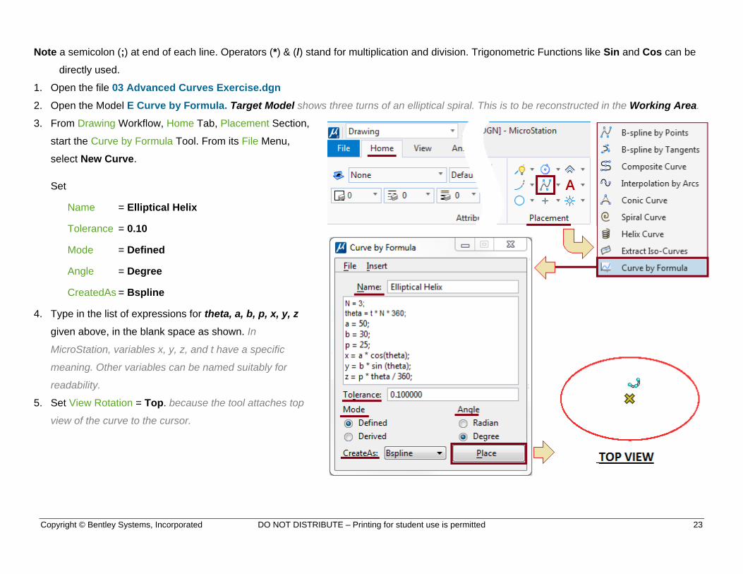
3. From Drawing Workflow, Home Tab, Placement Section,
start the Curve by Formula Tool. From its File Menu,
select New Curve.
Set
Name = Elliptical Helix
Tolerance = 0.10
Mode = Defined
Angle = Degree
CreatedAs = Bspline
4. Type in the list of expressions for theta, a, b, p, x, y, z
given above, in the blank space as shown. In
MicroStation, variables x, y, z, and t have a specific
meaning. Other variables can be named suitably for
readability.
5. Set View Rotation = Top. because the tool attaches top
view of the curve to the cursor.
Copyright © Bentley Systems, Incorporated DO NOT DISTRIBUTE – Printing for student use is permitted 24
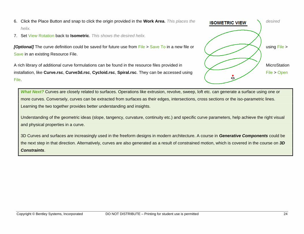
6. Click the Place Button and snap to click the origin provided in the Work Area. This places the desired
helix.
7. Set View Rotation back to Isometric. This shows the desired helix.
[Optional] The curve definition could be saved for future use from File > Save To in a new file or using File >
Save in an existing Resource File.
A rich library of additional curve formulations can be found in the resource files provided in MicroStation
installation, like Curve.rsc, Curve3d.rsc, Cycloid.rsc, Spiral.rsc. They can be accessed using File > Open
File.
What Next? Curves are closely related to surfaces. Operations like extrusion, revolve, sweep, loft etc. can generate a surface using one or
more curves. Conversely, curves can be extracted from surfaces as their edges, intersections, cross sections or the iso-parametric lines.
Learning the two together provides better understanding and insights.
Understanding of the geometric ideas (slope, tangency, curvature, continuity etc.) and specific curve parameters, help achieve the right visual
and physical properties in a curve.
3D Curves and surfaces are increasingly used in the freeform designs in modern architecture. A course in Generative Components could be
the next step in that direction. Alternatively, curves are also generated as a result of constrained motion, which is covered in the course on 3D
Constraints.