1

Benefits and Challenges of Over-Actuated Excitation Systems

Norman Fitz-Coy and Vivek Nagabhushan Michael T. Hale Department of Mechanical and Dynamic Test Branch Aerospace Engineering Redstone Technical Test Center University of Florida U.S. Army Developmental Test Command

This paper provides a comprehensive discussion on the benefits and technical challenges of controlling over-determined and over-actuated excitation systems ranging from 1-DOF to 6-DOF. The primary challenges of over-actuated systems result from the physical constraints imposed when the number of exciters exceeds the number of mechanical degree-of-freedom. This issue is less critical for electro-dynamic exciters which tend to be more compliant than servo-hydraulic exciters. To facilitate the technical challenges discussion, generalized methods for determining the drive output commands and the actuator input transform is presented. To further provide insights into the problem, over-actuated 1-DOF and 6-DOF examples are provided. Results are presented to support the discussions.

INTRODUCTION

Dynamic testing in a laboratory environment has long been a successful method of experimentally determining the mechanical properties of a structure as well as a technique for providing a degree of confidence that the unit under test (UUT) can structurally and functionally withstand a specified deployment environment. The simplest and most common laboratory vibration test consists of a single exciter providing motion in a single mechanical degree-of-freedom. However, there are many circumstances that will require use of multiple exciters to meet test objectives. A multiple exciter test (MET) is required whenever more than one mechanical degree-of freedom is required simultaneously, when a single actuator is not capable of addressing the test requirement, or possibly a combination of both scenarios. Clearly, one could envision unlimited combinations of actuator placements, actuator performance, and payload combinations. The use of MET has overlap into different disciplines including the automotive, aerospace, defense, and seismic communities [1-21]. Much of the early application of over-actuated 6-DOF excitation systems can be traced back to the seismic community. The designs were typically addressing very large payloads such as buildings or bridge structures with test bandwidths of interest generally in the DC to 50 Hz range. In recent years, the application of MET has become more wide-spread in the general dynamic test community yielding numerous systems with widely varying size and operational bandwidths. Many existing MET configurations are not over-actuated and control of these systems has been successful using a variety of commercially available control systems. Of primary interest, and the basis for the discussions within this paper, are the challenges associated with high bandwidth over-actuated MET configurations. Particular attention will be paid to the unique issues presented when designing and controlling wide bandwidth (up to 500 Hz) over-actuated servo-hydraulic systems. This paper is outlined as follows. First we motivate the need for over-actuated METs which is followed by an analysis of the kinematic constraints that are imposed by such systems. These discussions are followed by specific examples to highlight the characteristics of these systems. Finally we close with some recommendations for the community to consider.

2

PERFORMANCE CHARACTERISTICS OF SERVO-HYDRAULIC ACTUATORS

Essential performance parameters required to size a hydraulic exciter are peak velocity, displacement, peak force, and frequency response. Sizing a hydraulic exciter is also dependent upon the type of test to be conducted (i.e. sinusoidal, random, or shock). To illustrate how these performance parameters affect the sizing of a hydraulic exciter, an example is provided in terms of a sinusoidal test requirement. The example is intended to illustrate the significant effect in frequency response incurred as force requirements are increased. Refer to Table 1 as an example of actuator performance parameters associated with configuring an excitation system with a single vertical actuator vs. dual actuators.

Table 1 Hydraulic Exciter Performance Vert-1 Actuator Vert-2 Actuators

Force Required per Actuator 100% 66000 33000 lbfDynamic Pressure (Static *0.667) 4500 3000 3000 psi

Piston Diameter 5.3 3.7 inPiston Area 22.0 11.0 in^2Platform + Fixture 4000 4000 4000 lbsPayload 2000 2000 2000 lbsG-Peak 100% 10.00 10.00 G-PkVelocity Required 100% 35.00 35.00 ipsNumber of Actuators 1 2 eaMax Stroke 3.00 3.00 inDashpot Length 5% 0.30 0.30 inBulk Modulus of Oil (Beta) 175000 175000 175000 lb/in^2Volume Trapped Oil (includes dashpots) 73 36 in^3Oil Column Resonance 87.2 87.2 Hz

Peak FLOW REQUIRED per Actuator 200 GPM 100 GPMRMS FLOW REQUIRED per Actuator 67 GPM 33 GPM

V2 V1 LEGEND:Inches PK-PK 3.00 3.00 VARIABLE

G's PEAK 10.00 10.00 CALCULATEDV's PEAK 35.00 35.00 REFERENCE

Note: 1G added ot acceleration reference in all calculations to account for Gravity.

Reference Criteria Used in Calculations

The various fields in Table 1 are color coded in terms of desired reference values (orange), user defined variables (green), or calculated values (yellow). Observe that the displacement criteria is 3.0 inch DA, the peak velocity criteria is 35 in/sec, and the peak acceleration rating is 10G which for a user defined total mass of 6000 lb (4000 lb platform and fixture plus 2000 lb payload) yields a vertical axis force rating of 66000 lbf when considering gravity. There are two dominant factors that limit the frequency response of a servo-hydraulic exciter. The first factor is the natural frequency of the oil column. A good approximation of the oil column resonance is computed as:

π

=_

12oil columnn

oil

Tf

KM

where, β=

24oil

T

AK

V is the stiffness of the oil column, TV is the actuator volume including dashpots, β is the bulk

modulus of oil (default 175,000 lb/in2) and A is the piston area.

Physically, compression of the oil column can be viewed as a second order mechanical system which implies a -12 db/oct roll-off in performance at frequencies above the oil column resonance. In this example, for the dual actuator

3

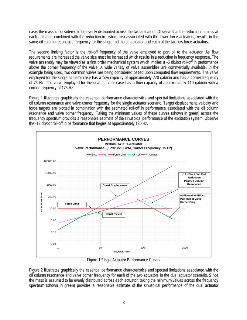
case, the mass is considered to be evenly distributed across the two actuators. Observe that the reduction in mass at each actuator, combined with the reduction in piston area associated with the lower force actuators, results in the same oil column resonance frequency for the single high force actuator and each of the two low force actuators. The second limiting factor is the roll-off frequency of the valve employed to port oil to the actuator. As flow requirements are increased the valve size must be increased which results in a reduction in frequency response. The valve assembly may be viewed as a first order mechanical system which implies a -6 db/oct roll-off in performance above the corner frequency of the valve. A wide variety of valve assemblies are commercially available. In the example being used, two common valves are being considered based upon computed flow requirements. The valve employed for the single actuator case has a flow capacity of approximately 220 gal/min and has a corner frequency of 75 Hz. The valve employed for the dual actuator case has a flow capacity of approximately 110 gal/min with a corner frequency of 175 Hz. Figure 1 illustrates graphically the essential performance characteristics and spectral limitations associated with the oil column resonance and valve corner frequency for the single actuator scenario. Target displacement, velocity and force targets are plotted in combination with the estimated roll-off in performance associated with the oil column resonance and valve corner frequency. Taking the minimum values of these curves (shown in green) across the frequency spectrum provides a reasonable estimate of the sinusoidal performance of the excitation system. Observe the -12 db/oct roll-off in performance that begins at approximately 180 Hz.

PERFORMANCE CURVESVertical Axis: 1-Actuator

Valve Performance: (Flow: 220 GPM, Corner Frequency: 75 Hz)

0.01

0.10

1.00

10.00

100.00

1000.00

10000.00

100000.00

1 10 100 1000FREQUENCY (Hz)

AC

CEL

ERA

TIO

N (G

)

Disp Vel Force Limit Oil Col V_Corner

Const Displacement

Const Pk Vel

-12 dB/oct Vel Perf Reduction

Past Oil ColumnResonance

Force Limit

Additional -6 dB/oct Perf Red at Valve Corner Freq .

Figure 1 Single Actuator Performance Curves

Figure 2 illustrates graphically the essential performance characteristics and spectral limitations associated with the oil column resonance and valve corner frequency for each of the two actuators in the dual actuator scenario. Since the mass is assumed to be evenly distributed across each actuator, taking the minimum values across the frequency spectrum (shown in green) provides a reasonable estimate of the sinusoidal performance of the dual actuator

4

configuration. Observe the -12 db/oct roll-off in performance for the lower force exciters employed in the dual actuator scenario begins at approximately 280 Hz. The use of dual actuators illustrated in this example result in a significant increase in bandwidth performance relative to the single actuator case.

PERFORMANCE CURVESVertical Axis: 2-Actuators

Valve Performance: (Flow: 110 GPM, Corner Frequency: 175 Hz)

0.01

0.10

1.00

10.00

100.00

1000.00

10000.00

100000.00

1 10 100 1000FREQUENCY (Hz)

AC

CEL

ERA

TIO

N (G

)

Disp Vel Force Limit Oil Col V_Corner

Const Displacement

Const Pk Vel

-12 dB/oct Vel Perf Reduction

past oil columnresonance

Force LimitAdditional -6 dB Perf Reduction at Valve Corner Freq .

Figure 2 Dual Actuator Performance Curves

The discussion within this section has been limited strictly to actuator performance. Omitted thus far are the details as to how multiple exciters may be configured. In the simple example provided, the two actuators could be configured, with proper mechanical constraints, such that either one or two mechanical degrees of freedom are possible. For the case in which two mechanical degrees-of-freedom are possible, control is readily achievable via multiple commercially available MDOF vibration control software products. The over-actuated cases in which the two hydraulic actuators are configured to obtain a single mechanical degree-of freedom introduce additional control concerns. It is the general over-actuated case employing hydraulic actuators that is the main subject of the sections that follow.

IMPLEMENTATION CONSIDERATIONS FOR OVER-DETERMINED AND OVER-ACTUATED EXCITATION SYSTEMS

Consider a typical MET vibration system with d actuators, n measurements, and m motion degrees-of-freedom (DOFs). A block diagram of a typical MET vibration system is shown in Figure 3. For the traditional single-degree-of-freedom system, blocks A and B would simply be unity and not exist. For the over-determined case, the number of measurements (accelerometer output channels) exceeds the number of motion DOFs of the system (i.e., >n m ) and thus requires a method for extracting the motion information from the measurements. This process is shown in Block A and is referred to as “input” transform” in the literature [4]. Similarly for the over-actuated case, the excitation system contains more actuators that motion DOF (i.e. >d m ), implying the need for coordination between the

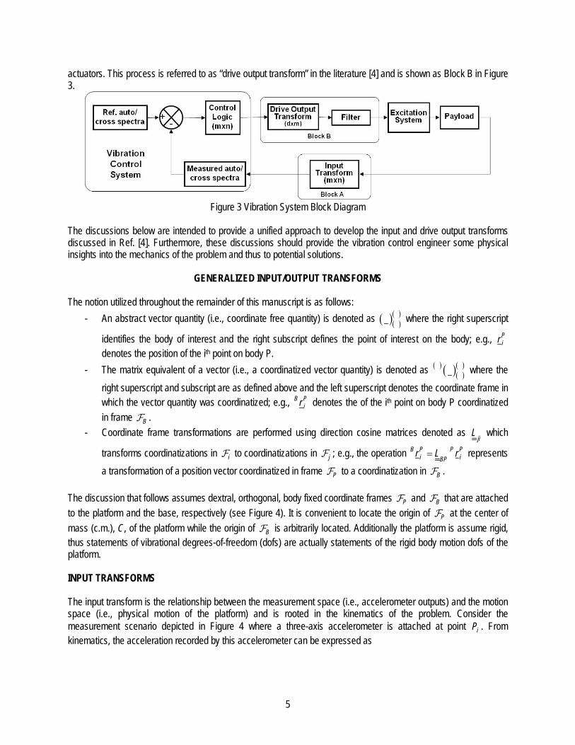
5

actuators. This process is referred to as “drive output transform” in the literature [4] and is shown as Block B in Figure 3.

Figure 3 Vibration System Block Diagram

The discussions below are intended to provide a unified approach to develop the input and drive output transforms discussed in Ref. [4]. Furthermore, these discussions should provide the vibration control engineer some physical insights into the mechanics of the problem and thus to potential solutions.

GENERALIZED INPUT/OUTPUT TRANSFORMS The notion utilized throughout the remainder of this manuscript is as follows:

- An abstract vector quantity (i.e., coordinate free quantity) is denoted as ( )( )( ) where the right superscript

identifies the body of interest and the right subscript defines the point of interest on the body; e.g., Pir

denotes the position of the ith point on body P. - The matrix equivalent of a vector (i.e., a coordinatized vector quantity) is denoted as ( ) ( )( )

( ) where the right superscript and subscript are as defined above and the left superscript denotes the coordinate frame in which the vector quantity was coordinatized; e.g., B P

ir denotes the of the ith point on body P coordinatized in frame B .

- Coordinate frame transformations are performed using direction cosine matrices denoted as ji

L which

transforms coordinatizations in i to coordinatizations in j ; e.g., the operation =B P P Pi iBP

r L r represents a transformation of a position vector coordinatized in frame P to a coordinatization in B .

The discussion that follows assumes dextral, orthogonal, body fixed coordinate frames P and B that are attached to the platform and the base, respectively (see Figure 4). It is convenient to locate the origin of P at the center of mass (c.m.), C, of the platform while the origin of B is arbitrarily located. Additionally the platform is assume rigid, thus statements of vibrational degrees-of-freedom (dofs) are actually statements of the rigid body motion dofs of the platform. INPUT TRANSFORMS The input transform is the relationship between the measurement space (i.e., accelerometer outputs) and the motion space (i.e., physical motion of the platform) and is rooted in the kinematics of the problem. Consider the measurement scenario depicted in Figure 4 where a three-axis accelerometer is attached at point iP . From kinematics, the acceleration recorded by this accelerometer can be expressed as

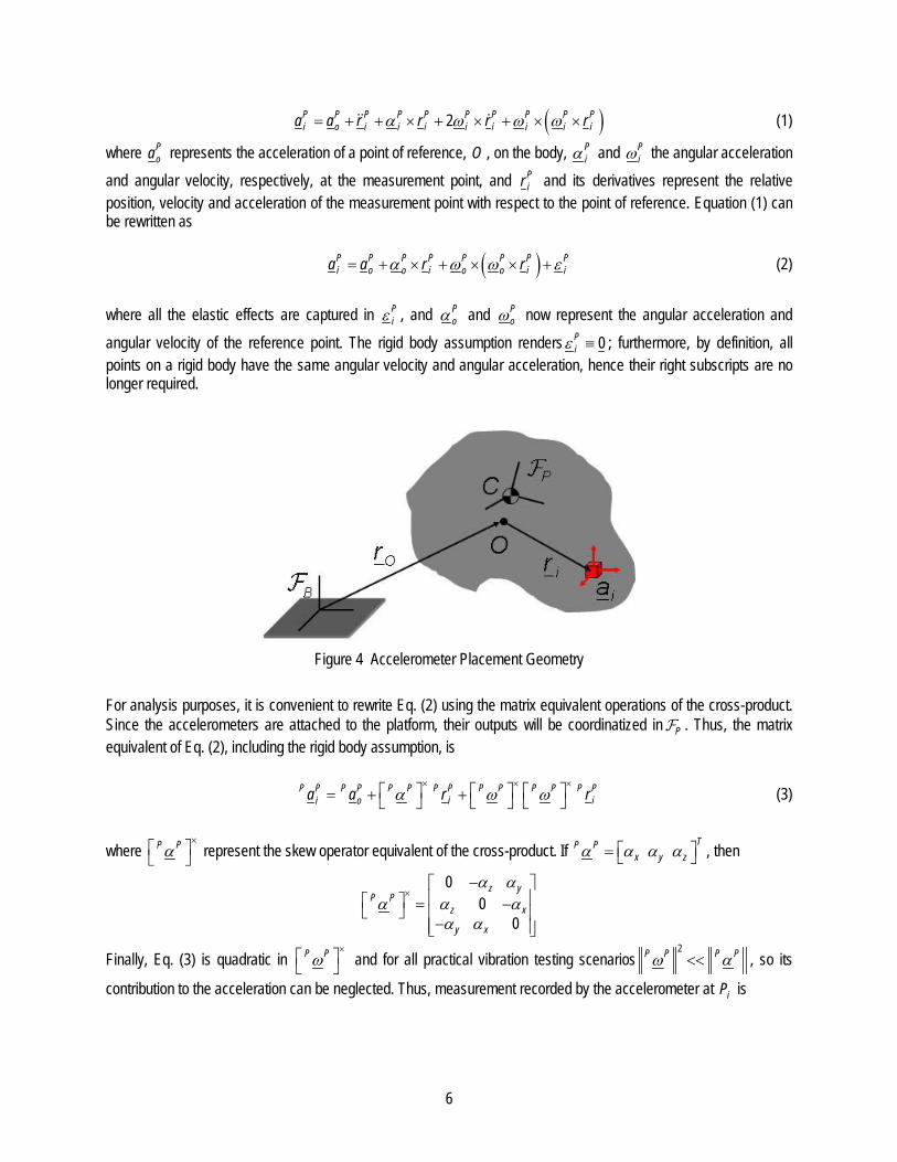
6

( )α ω ω ω= + + × + × + × × 2P P P P P P P P P Pi i i ii o i i i ia a r r r r (1)

where Poa represents the acceleration of a point of reference, O , on the body, α P

i and ωPi the angular acceleration

and angular velocity, respectively, at the measurement point, and Pir and its derivatives represent the relative

position, velocity and acceleration of the measurement point with respect to the point of reference. Equation (1) can be rewritten as ( )α ω ω ε= + × + × × +P P P P P P P P

i ii o o o o ia a r r (2) where all the elastic effects are captured in ε P

i , and α Po and ωP

o now represent the angular acceleration and angular velocity of the reference point. The rigid body assumption rendersε ≡ 0P

i ; furthermore, by definition, all points on a rigid body have the same angular velocity and angular acceleration, hence their right subscripts are no longer required.

Figure 4 Accelerometer Placement Geometry

For analysis purposes, it is convenient to rewrite Eq. (2) using the matrix equivalent operations of the cross-product. Since the accelerometers are attached to the platform, their outputs will be coordinatized in P . Thus, the matrix equivalent of Eq. (2), including the rigid body assumption, is

α ω ω× × ×

= + + P P P P P P P P P P P P P P

i ii oa a r r (3)

where α×

P P represent the skew operator equivalent of the cross-product. If α α α α = TP P

x y z , then

α α

α α αα α

×−

= − −

00

0

z yP P

z x

y x

Finally, Eq. (3) is quadratic in ω×

P P and for all practical vibration testing scenarios ω α<<2P P P P , so its

contribution to the acceleration can be neglected. Thus, measurement recorded by the accelerometer at iP is

7

α α× ×

= + = − P P P P P P P P P P P P P P

i ii o oa a r a r (4) Equation (4) is an expression for the three components of the acceleration at the measurement point. In practice only select components of the measurement are utilized. To extract this information from Eq. (4) we define the following row selection matrices: [ ]= 1 0 0T

xe , [ ]= 0 1 0Tye , and [ ]= 0 0 1T

ze . For example, the kth accelerometer measurement representing the y-component of acceleration at iP is

α

α

×

×

= −

= −

yT P P P P P P

ik y o

P PoT T P P

iy yP P

a e a r

ae e r

In general, the measurement components are

α

× = −

j

P PoT T P P

ik j jP P

aa e e r (5)

where ( )∈ 1, 2, ...,k n , ( )∗∈ 1, 2, ...,i n and ( )∈ , ,j x y z . Parameter n represents the number of accelerometer

measurements (as previously defined) and ∗ ≤n n the number of measurement location; e.g., utilization of multi-axis accelerometers results in ∗ <n n . Equation (5) represents one equation in six unknowns, the three components of the acceleration of the reference point and the three components of the rigid body angular acceleration. In order to determine these quantities, at least six measurements are needed. These requirements are not as stringent as that reported in Ref [24] because of the assumptions above (i.e., small angular velocities and rigid body). Let’s consider the most general case of n-measurements from n* locations. In this case, Equation(5) becomes

( )( )

( )α

∗

×

×

× ×

××

− − = =

−

11

2

6 11

6

j

jj

j

T T P Pj j

P PT T P P o

ij jk

P P

n T T P Pj jn n

n

e e raaa e e ra

ae e r

, ( ) ( ) ∗∈ ∈1, 2, ..., , , ,i n j x y z

which is of the form [ ]

( ) ( )[ ]( )× ××

= 1 6 16

meas motionn n

(6)

Equation (6) can be rewritten as [ ] [ ][ ]=motion meas (7) where [ ]motion is a 6x1 matrix of unknown linear and angular accelerations, [ ]meas is an nx1 matrix of measurements (known), and [ ] is a 6xn matrix referred to in the literature as the “Input Transform”.

8

Observe that is entirely defined by knowledge of (i) placement, (ii) orientation, and (iii) utilized signals of the

accelerometers. Since [ ] ( )− = 1T T

, the Input Transform can always be determined provided

has full column rank, which is entirely dependent on the placement of the accelerometers. For example, will be rank deficient if accelerometers providing z-axis outputs are positioned such that the x- and y-components of their position vectors are identical. This is apparent by observing the rows of corresponding to these measurements

are [ ]×

= − 0 0 1 0T T P Pi i iz ze e r y x , implying that no additional information is provided by addition of these

rows. Similar arguments exist for the x-axis and y-axis measurements. In practice care must be taken when positioning the accelerometers since misalignments in their orientation and imprecise knowledge of their locations will affect the elements of the input transform matrix. For small angular misalignments (< °10 ), the effect can be ignored as is shown in below. Denoting the small angular misalignments as θx , θy , and θz , then the transformation matrix from the “perfectly” aligned (ideal) frame to the misaligned (actual)

frame is approximated [] as ( )θ ×= −1L where ( )θ θ θ θ=T

x y z . Thus, for example, a row selection to extract the x-component of acceleration, becomes

θ θ

θ θ θθ θ θ

− = − = − −

1 1 11 0

01act

z y

z x zx

y x y

e

which shows that the actual and ideal selected rows are identical. Similar arguments can be made for the other two directions. However, the angular misalignment effect must be included for large angles since the approximation for the transformation matrix becomes invalid and a cosine relationship ensues. The effects of errors in the knowledge of the accelerometer’s position can be seen from Eq. (5). Let the position be δ+P P P P

i ir r , then the measured (meas) and computed (comp) are related by

δα

δα α

×

× ×

= − +

= − + −

= +

0

jmeas

j jcomp error

P PoT T P P P P

ik j j iP P

P P P Po oT T P P T P P

ij j j iP P P P

k k

aa e e r r

a ae e r e r

a a

DRIVE OUTPUT TRANSFORMS Over-actuated MET scenarios occur if the use of more than one exciter is required to address a single rigid body DOF. Such a situation may occur when either (i) a single exciter may not be of sufficient power to address the test specifications, (ii) the size of the UUT may require multiple attachment points, or (iii) possibly existence of both conditions. Figure 5 shows the geometry of the problem under consideration. Each actuator has one end attached to the platform and the other attached to the base (see Fig. 5a). iP denotes the attachment point of the ith actuator in the platform and iB the attachment point of the same actuator in the base. Dextral, orthogonal, body fixed coordinate

9

frames P and B are defined in the platform and the base, respectively (see Fig. 5b). It is convenient to locate the origin of P at the center of mass (c.m.), PC , of the platform while the origin, O, of B can be arbitrarily located.

CB

CP

B1B2

B3

Br

P1

P2 P3 Pr

Base

Platform

1F

2F

3FrFW

(a)

CB

CP

Bi

O

R

Pi

Base

Platform

ˆ ii uσ

Bir

Pir

iF

iM

P

B

(b) Figure 5 Generalized Multi-Axis Vibration System

The force exerted on the platform by the ith actuator can be expressed as = ˆi i iF f u (8) where if is the magnitude of the exerted force and ˆ iu is a unit vector in the direction of the line of action (LOA) of the force (also known as line coordinates [26, 27]). As shown in Fig. 5b, the unit LOA vector is

( )σ= − +

1ˆ P Bi ii

iu r r R

where Pir and B

ir are the position vectors of iP and iB , respectively; R specifies the location of the origin of B relative to the origin of P and σ i is the magnitude of the LOA vector. It is convenient to coordinatize ˆ iu in B , thus

( )σ= − +

1ˆB P P B B Bi ii BP

iu L r r R (9)

where = TP P P P P

i i i ir x y z , = TB B B B B

i i i ir x y z and [ ]= TB R X Y Z . The convenience of coordinatizing in B

is based on the fact that for most vibration test systems utilize fixed LOA actuators and thus ˆBiu can be determined

from inspection (see examples discussed below). However, the expression in Eq. (9) is applicable for both fixed and variable (e.g., Stewart platform configurations) LOA systems. From Newton’s second law, the translational motion of the platform is governed by

( ) = = + +∑P PC i EC

i

d mv ma F W Fdt

(10)

10

=W mg in Eq. (10) represents the weight and EF represents all other external forces that act on the platform. For most vibrational systems, the external forces can be assumed to be zero and since the translation motion represents the linear motion of the platform relative to the base, it is convenient to coordinatize Eq. (10) in B and rewrite as ( )= −∑ B B P B

i Ci

F m a g (11)

Equation (11) can be rewritten in terms of the LOA vectors as

( )

= −

1

21 2ˆ ˆ ˆB B B B P B

d C

d

ffu u u m a g

f

(12)

In general iP does not coincide with the platform’s c.m., thus the actuator generates a moment (torque) about the platform's c.m. given by = × = × =ˆP P P

i i i i ii iiM r F r f u m f (13)

Pim is known as the moment arm of if and is the normal to the plane containing the LOA of the ith force and the

vector from the origin to the point of application of the force. It is convenient to coordinatize Eq. (13) in P as =P P P

i i iM m f , with the column matrix P Pim obtained from the skew matrix equivalent of the vector cross product

×

− = = − −

0ˆ ˆ0

0

P Pi i

B BP P P P P Pi i i ii iPB PB

P Pi i

z ym r L u z x L u

y x (14)

Here PB

L represents the transformation (direction cosine matrix) from the base coordinates ( B ) to the platform coordinates ( P ). Euler’s equations provide the governing equations for rotational motion. When applied about the cm of the platform (or an inertial point), Euler’s equations are

( ) = +∑PC i E

i

d H M Mdt

(15)

where ω= ⋅P P P

C CH I is the angular momentum of the platform about its c.m. and EM is the external torque

associated with EF (assumed zero). The weight acts through the c.m. and therefore produces no moment about that point. Since we are interested in the attitude (orientation) of the platform with respect to the base, it is convenient to coordinatize Eq. (15) in P . Substituting the expression for angular momentum into Eq. (15), neglecting the external moments and coordinatizing the resulting expression in P yields

11

( )ω ω ω×

= + −

1

21 2

P P P P P P P P P P P P P P P Pd EC C

d

ffm m m I I M

f

(16)

The translational and rotational motions of the platform are combined using Eqs. (12) and (16) to obtain a relationship between the actuator forces and the ensuing motion

( )

( )ω ω ω×

− − = + −

1

1 2 2

1 2

ˆ ˆ ˆB P B BB B B ECd

P P P P P P P P P P P P P P P Pd EC C

d

fm a g Fu u u f

m m m I I Mf

(17)

Equation (17) is of the form [ ][ ] [ ]

× × ×

=(6 d) (d 1) (6 1)P F C (18)

where [ ]P is a matrix of line coordinates and moment arms which is referred to as the matrix of Plucker coordinates [26, 27], [ ]F is a matrix of actuator force magnitudes, and [ ]C is the matrix of the desired motion command (i.e., the generalized inertia force). Equation (18) can be interpreted in the following manner – given the desired motion [ ]C , determine the actuator force commands [ ]F required to generate that motion. There are two cases of interest, under-actuated ( ≤d m ) and over-actuated ( >d m ) systems where ≤ 6m in both cases. We examine each case separately. Under-actuated System: In Ref. [23] a singular value decomposition (SVD) analysis was used to show that the under-actuated case < ≤ 6d m actuators have, at most, control authority over d dofs (i.e., d actuators can at best excite d dofs in a

controllable manner). The analysis is repeated here for completeness. Via the SVD, [ ]P can be represented as [ ] = Σ TP U V , where U and V are respectively, (6x6) and (dxd) unitary matrices. Assuming that [ ]P has full column rank (i.e., there are no redundant actuators), then Σ has the form

( )σ σ

Σ = −−−−−−−− −

1, , }

0 6}

ddiag d

d

Substituting [ ] = Σ TP U V into Eq. (18) and premultiplying both sides by TU yields

( )

[ ] [ ]σ σ

− −−−−−−− =

1, ,

0

r T Tdiag

V F U C (19)

where one observes that the lower ( )−6 d rows of Eq. (19) are zero. This suggests Eq. (19) can be partitioned as

12

[ ] − − = −−

U U

L R

P CF

P C (20)

where the desired motion is given by [ ][ ] [ ]=U UP F C and the actuator commands are uniquely determined since [ ]UP is full rank. The lower partition, [ ][ ] [ ]=L RP F C , describes residual motion that may occur; typically this motion is zero, but if it does occur, it is NOT controllable. Since the actuator commands are linearly independent, the required input transform is the identity matrix. It should be noted that if [ ]P does not have full column rank, then the system is over-actuated (i.e., the input commands are not linearly independent) and those cases are discussed below. Over-Actuated System: For an over-actuated system ( >d m ), the partitioning of the Plucker matrix as discussed above does not occur since its rank is now based on row rather than columns. For these systems, the drive commands for the d actuator force inputs are not linearly independent and are related to a linearly independent set of m drive commands by [ ] [ ] [ ]

× × ×

=( 1) ( ) ( 1)

T

d d m mF P D (21)

Here [ ]D is the ( )≤ 6m independent drive commands, [ ]F is the >d m dependent drive commands, and [ ]TP is referred to in the literature as the “drive output transform” [4]. Substituting into Eq. (18), the independent drive command can be determined from the motion command as

[ ] [ ][ ]( ) [ ]−

=1TD P P C (22)

which can then be substituted into Eq. (21) to determine the dependent actuation force levels from

[ ] [ ] [ ] [ ] [ ][ ]( ) [ ]−

= =1T T TF P D P P P C (23)

Of course, Eq. (23) represents the Moore-Penrose pseudo inverse of Eq. (18), but the development presented above highlights the physical intuition that a set of linearly independent drive commands exists. Such insights would have been foreshadowed if the pseudo inverse had been directly applied. The drive output transform matrix contains a wealth of information regarding the system’s performance. First, if [ ]P

is of full row rank, [ ][ ]TP P is a full ranked ×m m matrix, thus its inverse exits; i.e., the independent drive command [ ]D can always be determined. Second, the mechanical advantage provided by the configuration can be gleamed from this matrix. Third, the conditioning of [ ]P (i.e., the ratio of largest to smallest singular value) is an indication of the ability of the actuators to produce the desired motion. A lower condition number is an indication of a better actuator placement design. Finally, the null space of [ ]P describes the actuation combinations that will produce no rigid body motion of the platform. However, it is possible that combinations of motion defined by the null space still have the potential to excite flexible body modes. These properties will be discussed, from a rigid body perspective, in the examples that follow.

13

CASE STUDIES

Case 1: One Mechanical Degree-of-Freedom ( = = =2, 2, 1d n m ) Consider the over-actuated system shown in Figure 6. The mechanical degree of freedom of the system is a rotation θ about an axis out of the paper passing through the pivot point O . This degree of freedom is actuated by two hydraulic actuators at distances 1l and 2l from O along the length of the beam. There are two accelerometers that are placed on the beam for feedback at distances 1r and 2r from the pivot point along the length of the beam.

Actuator 2 Actuator 1

Pivot

Accelerometer 1 Accelerometer 2

Beam

x

X

Y

Z

y

z

O

1( )l

2( )l

1f 2f

θ 1r

2r

Figure 6 Single degree of freedom over-actuated system

Input Transform For this problem, the accelerometers are located by [ ]=1 1 0 0 TP Pr r and [ ]=2 2 0 0 TP Pr r with both recording

measurements in the y-direction. Thus α× = −

0y

T T P Pii y y

aa e e r from which Eq. (6) yields

α =

1 1 0

2 2

0 1 0 0 00 1 0 0 0

y

y

a r aa r

By choosing the reference point as the pivot point, then ≡0 0a and thus the first three columns of the coefficient

matrix can be eliminated. Further, since [ ]α α= 0 0 Tz , columns four and five of the coefficient matrix can also be

eliminated which results in

α =

1 1

2 2

y

yz

a ra r

Thus, = 1

2

rr from which the Input Transform matrix is determined as

[ ] ( )− = = + +

11 2

2 2 2 21 2 1 2

T T r rr r r r

Drive Output Transform For this problem, the relevant geometric properties for the input forces are: [ ]=1 1 0 0 TP Pr l , [ ]=2 2 0 0 TP Pr l ,

[ ]=1ˆ 0 1 0 TB u , [ ]=2ˆ 0 1 0 TB u . The moment arm of each actuator about the pivot point (a fixed point) is

14

θ θθ θ

θ

× = = − − =

0 0 0 cos sin 0 0 0 0ˆ 0 0 sin cos 0 1 0 0

0 0 1 0 cos0 0

BP P P Pi i iiPB

i ii

m r L u ll ll

Since only rotational motion exists, the translational components of Eq. (17) can be neglected to get

ω ω ω× × = = + +

1 11 2

2 21 2

0 00 0P P P P P P P P P P P P P P

cO Of fm m J J m r gf fl l

where P Pcr defines the position of the platform’s c.m. with respect to the pivot point and [ ]θ θ= sin cos 0 TP g g is

the gravity vector coordinatized in P . The third term on the right represents the contribution of the platform’s mass to the angular momentum about point ‘O’. In the previous developments this term was zero because the moments were computed about the c.m thus eliminating its contributions. However, in this example the moments were determined about the pivot point (an inertial point), the contribution of the weight to the moment about that point must be included. Observe that the first two rows of the Plucker matrix are associated with the x- and y-rotational dofs and can be ignored since such motions are constrained (as shown by the equation). Thus, [ ] [ ]= 1 2P l l from which the drive command is

[ ] [ ][ ]( ) [ ] [ ]

[ ]

θ θ

ω θ

−− = = + = +

+

111

1 22

2 21 2

cos

1 cos

Tz c

z z c

lD P P C l l J mgll

J mgll l

The Drive Output transform [ ] = 1

2

T lP l and the actuation level is

[ ] [ ] [ ] θ θ = = = + + 1 1

2 22 21 2

1 cosTz c

f lF P D J mglf ll l (24)

The mechanical advantage of the configuration is +2 21 2l l and is inferred from [ ][ ]TP P .

Case 2: Six Mechanical Degrees-of-Freedom The example below is from Ref [4]. The geometry for the example is shown in Figure 5 from which the following definitions were extracted. [ ]= = −1 8 0 TP P P Pr r l l , [ ]= = −2 6 0 TP P P Pr r l l , [ ]= =3 5 0 TP P P Pr r l l , [ ]= = − −4 7 0 TP P P Pr r l l

[ ]=1ˆ 1 0 0 TB u , [ ]= −2ˆ 1 0 0 TB u , [ ]= −3ˆ 0 1 0 TB u , [ ]=4ˆ 0 1 0 TB u

[ ]= = = =5 6 7 8ˆ ˆ ˆ ˆ 0 0 1 TB B B Bu u u u

15

Figure 5 Geometry: (a) Actuator and sensor positions [4], (b) Position vectors

It should be noted that while this example discusses co-located actuation and measurement points, co-location is not a requirement of the formulation. By this we mean the positions vectors for the accelerometer locations do not have to be the same as that define the actuator positions. In practice co-located sensors and actuators maybe helpful in trouble-shooting but is not required. Input Transform In this configuration, single axis accelerometers are aligned with the actuators; e.g., at the upper right corner defined by vector 1

Pr has accelerometers that record measurements in negative y-direction and the positive z-direction. Using the formulation of Eq. (5) the following component definitions are obtained:

[ ]α α

× = − = −

11 1 0 0 0 0

x

P P P Po oT T P P

x xP P P P

a aa e e r l

[ ]α α

× = − = − −

22 1 0 0 0 0

x

P P P Po oT T P P

x xP P P P

a aa e e r l

[ ]α α

× = − = − −

33 0 1 0 0 0

y

P P P Po oT T P P

y yP P P P

a aa e e r l

[ ]α α

× = − = −

44 0 1 0 0 0

y

P P P Po oT T P P

y yP P P P

a aa e e r l

[ ]α α

× = − = −

55 0 0 1 0

z

P P P Po oT T P P

z zP P P P

a aa e e r l l

[ ]α α

× = − = − −

66 0 0 1 0

z

P P P Po oT T P P

z zP P P P

a aa e e r l l

16

[ ]α α

× = − = −

77 0 0 1 0

z

P P P Po oT T P P

z zP P P P

a aa e e r l l

[ ]α α

× = − =

88 0 0 1 0

z

P P P Po oT T P P

z zP P P P

a aa e e r l l

Combining these components as shown in Eq. (6) gives an which yields the input transform upon inversion

[ ]

− − =

− − − −

− − − −

.5 .5 0 0 0 0 0 00 0 .5 .5 0 0 0 00 0 0 0 .25 .25 .25 .250 0 0 0 .25 .25 .25 .250 0 0 0 .25 .25 .25 .25

.25 .25 .25 .25 0 0 0 0

l l l ll l l l

l l l l

where the first three rows are associated with the x-, y-, and z-translational accelerations, and the last three rows are associated with the x-, y-, and z-angular accelerations. Drive Output Transform The corresponding input is [ ] [ ]= 1 2 3 4 5 6 7 8

TF f f f f f f f f where 1f and 2f are in the x-direction forces at diagonally opposing corners, 3f and 4f are the y-direction forces applied at the corners of the other diagonal, and −5 8f f are vertical (z-direction) forces. Assuming small angular displacements of the platform, Eq. (14) can be used to obtain ( )θ θ ψ= − − 1 1 TP Pm l l l , ( )θ θ ψ= − − 2 1 TP Pm l l l , ( )φ φ ψ= − − 3 1 TP Pm l l l ,

( )φ φ ψ= − − 4 1 TP Pm l l l , ( )θ φ= − + 5TP Pm l l l , ( )θ φ= − − − − 6

TP Pm l l l ,

( )θ φ= − − + 7TP Pm l l l , ( )θ φ= − 8

TP Pm l l l Thus, the matrix of Plucker coordinates is

[ ] θ θ φ φθ θ φ φψ ψ ψ ψ θ φ θ φ θ φ θ φ

− − =

− − − − − −

− − − − − − − − + − − − + −

1 1 0 0 0 0 0 00 0 1 1 0 0 0 00 0 0 0 1 1 1 1

(1 ) (1 ) (1 ) (1 ) ( ) ( ) ( ) ( )

P l l l l l l l ll l l l l l l l

l l l l l l l l

The results of Ref [4] assumes the angular displacements are zero, so to be consistent we apply the same conditions to reduce the matrix of Plucker coordinates to

[ ]

− − =

− − − −

− − − −

1 1 0 0 0 0 0 00 0 1 1 0 0 0 00 0 0 0 1 1 1 10 0 0 00 0 0 0

0 0 0 0

P l l l ll l l l

l l l l

from which the Drive Output transform is determined as

17

[ ]

− − − − −

− =−

− − −

1 0 0 0 01 0 0 0 0

0 1 0 0 00 1 0 0 00 0 1 00 0 1 00 0 1 00 0 1 0

T

llllP l l

l ll l

l l

For the drive output transform shown above, the first three columns are associated, respectively, with the x-, y-, and z-translational dofs and the last three columns are associated with the x-, y-, and z-rotational dofs of the platform. With considerations for the appropriate physical degrees of freedom, the drive output transform shown in Eq. (3) of Ref. [4] is identical to that shown above. The mechanical advantage provided by the configuration is obtained from an evaluation of [ ][ ]TP P . For this example, we have [ ][ ] diag =

2 2 22 2 4 4 4 4TP P l l l which indicates that there is a mechanical advantage of 2 for the x- and y-translational dofs and an advantage of 4 for the z-translation and all three rotational dofs. Of course this result could have been discerned from careful examination of the actuator configuration. For this example, the null space of [ ]P contains the following two vectors:

[ ] [ ]= − −1

0 0 0 0 0.5 0.5 0.5 0.5 TnullF [ ] [ ]= − −

20.5 0.5 0.5 0.5 0 0 0 0 T

nullF In terms of rigid body motion, the scenario defined by the first null vector results in the four base actuators producing zero vertical force, pitch, and roll moments. Similarly, that of the second null vector involves the planar actuators producing no net horizontal forces and no yaw moment. Again, it is important to recognize that null space excitation has the potential to excite flexible body DOFs. Specific to this example, [ ]

1nullF corresponds to vertical actuators that are 180 degrees out of phase with respect to each other which may result in torsional deformation of the platform and [ ]

2nullF corresponds to out of phase horizontal exciters which may result in shear deformation of the table, as discussed in [4]. . Case 3: One Mechanical Degree-of-Freedom with Phase Difference The purpose of this example is to highlight the effects of actuator phase difference on the performance of the system. This is demonstrated by considering sinusoidal inputs 1f and 2f which cause displacements 1y and 2y at the actuator attachment points of example Case 1. To further highlight these effects, we consider two different actuation systems: (i) electrodynamic actuation and (ii) hydraulic actuation (Fig. 6). In the case of ideal actuators that can be phase matched, it is possible that the forces are in phase and follow the relationship as given by Eq. (24), Equation (25) provide the actuation conditions for rigid body motion (neglecting inertia effects).

ω

ω

=

=

1 1

2 2

sin( )

sin( )

f

f

f F t

f F t

ω

ω

=

=

1 1

2 2

sin( )

sin( )

y Y t

y Y t (25)

18

where ωf is the frequency of actuation, 1Y and 2Y are the peak displacements consistent with the motion. However, for realizable systems, it is difficult to phase match the actuators and thus the imparted forces will have some phase, differences and produce displacements which may not be consistent with rigid body motion. The motion of the attachment points become functions of generalized displacement functions 1q and 2q given by ω

ω φ=

= +1 1

2 2

sin( )sin( )

ff

f F tf F t ω φ

ω φ==

1 1 1 22 2 1 2

( , , , , , )( , , , , , )

ff

y q E I F Fy q E I F F (26)

where φ represents the actuation phase difference, E and I are the beam’s Young’s modulus and its second moment of the cross-sectional area. This difference in displacement will cause structural deformations in the beam leading to high actuator forces and excitation of some modes of the beam. Figure 6 in considers two cases of actuation of a beam – one by an electrodynamic actuator and the other by a hydraulic shaker. In the common case let the forces by actuators 1 and 2 at distances 1l and 2l cause displacements 1y and 2y at the attachment points. If ( )≠1 1 2 2y l l y , which is the condition for rigid body motion then the beam has to flex to comply with the displacements. For the electrodynamic actuator case, the magnet field/armature acts as a compliant spring that would compensate for the displacement difference and does not let the beam to deform. Due to the compliance of the spring, 1y will now be equal to ( ) ( )( )= + ∆ = −∆1 1 1 2 2/E Ey y s l l y s . The additional force on the beam would be only ( )∆k s where k is the stiffness of the beam.

(A) (B) Figure 6 Comparison between (a) Electrodynamic and (b) Hydraulic actuators

For the case of the hydraulic oil column is stiff and not compliant enough to avoid considerable beam deformations. This causes the beam to deflect by the difference in displacements between the rigid body motion to the actual displacement. The additional force now is considerable as the bending stiffness of the beam is high. This additional force on the actuator may also damage the valves in the hydraulic circuit. A test case with the following specifications of the beam was simulated in ADAMS software [28].

Beam length: 1m Beam cross-section: 0.05m X 0.05m Beam material: steel Density of the beam: 7800 Kg/m3

Actuator 1 Actuator 2

1Ey s+ ∆ 2Ey s− ∆

19

Young modulus: 210 Gpa Position of the actuators: =1 0.4ml and =2 0.8ml

In the first case the actuator was modeled with a spring in series to simulate the electrodynamic actuator. The stiffness of the spring used was 10N/mm with a damping ratio of 0.1. Figure 7 shows the plot of the forces at the electrodynamic actuator joints when the actuators are (a) in phase and (b) out of phase by π radians. The simulation was repeated with the springs replaced by a rigid member to represent the hydraulic actuator. Figure 8 shows the plot of the forces at the hydraulic actuator joints when the actuators are (a) in phase and (b) out of phase by π radians.

Figure 7 Electrodynamic actuator simulation

20

Figure 8 Hydraulic actuator simulation

It is evident from the above plots that there is an enormous increase in the forces at the actuator joints due to the flexure of the beam in case of a hydraulic actuator. This problem does not occur in case of an electrodynamic actuator due to the compliance by the actuator springs.

DISCUSSIONS AND CONCLUSIONS In this paper we have motivated the need for over-actuated vibration control systems and discussed the challenges that are present in multi-axis vibration systems. The relationships between the desired vibrational motion and the actuation required to generate that motion is developed from a mechanics perspective and used to highlight the challenges that exist for these systems. Based on these relationships, we have shown that a drive output transform is not required for under-actuated systems but is essential for over-actuated. Due to the use of electro-dynamic actuators, the need for drive output transforms in over-actuated systems were not as critical since the actuator itself provide the compliance required if the drives were not synchronized. However, as the use of hydraulic actuators become more prevalent in these over-actuated systems, it will be imperative that such transforms be integrated into the development of the control systems since these actuators will not provide the necessary compliance. Actuator developers are currently investigating passive methods for providing some compliance (e.g., TEAM’s delta-P valve),

21

however, such devices will not in principle provide the necessary compliance required for over-actuated systems. Such devices would provide the necessary compliance associated with proper drive commands sent to excites with slightly different response characteristics. Furthermore, the use of drive output transforms to provide the correct drive signals will mitigate the excitation of the platform’s vibratory modes during a test. While employing the information obtained from the input and output transformations provides the foundation for controlling rigid body motion, it is also important to recognize that the mechanical impedance of a laboratory system will generally not be exactly the same as the field conditions from which the original measurements were acquired. Generally, there will be some spectral smoothing associated with over-determined feedback. It may also be necessary to include additional measurement points to be used as notching channels in the event the laboratory impedance mismatch results in undesired response dynamics.

22

References 1. K. A. Edge, “The control of fluid power systems - responding to the challenges,” Proc. Institution of Mechanical.

Engineers, Part I: J. Systems and Control Engineering, 1996, 211, 91-110. 2. M Tochizawa, K A Edge, “A comparison of some control strategies for a hydraulic manipulator,” Proc. Of the

American Controls Conference, San Diego, California June 1999, pp. 744-748 3. T. Davis, “Multiple-Input, Multiple-Output (MIMO) Control Systems - A New Era in Shaker Control,” Sound and

Vibration, Jan. 2006. 4. M. Underwood and T. Keller, “Applying Coordinate Transformations to Multi-DOF Shaker Control,” Sound and

Vibration, Jan. 2006, pp 22-27. 5. F. De Coninck, W. Desmet, P. Sas, “Increasing the Accuracy of MDOF Road Reproduction Experiments:

Calibration, Tuning and a Modified TWR Approach,” Proc. of the International Conference on Noise and Vibration Engineering, Sept. 2004, pp.709-722

6. J. Zhao, C. French, C. Shield, and T. Posbergh, “Considerations for the development of real-time dynamic testing using servo-hydraulic actuation,” Earthquake Engineering Structural Dynamics, 2003; 32, pp. 1773–1794.

7. J. Zhao, C. Shield, C. French, and T. Posbergh, “Effect of Servo Valve/Actuator Dynamics on Displacement Controlled Testing,” Presented at the 13th World Conference on Earthquake Engineering, Vancouver, B.C., Canada, August 1-6, 2004, Paper No. 267

8. H. Hahn, K.-D. Leimbach, “Nonlinear Control and Sensitivity Analysis of A Spatial Multi-Axis Servo-Hydraulic Test Facility,” Proc. Of the 32nd Conference on Decision and Control, San Antonio TX, Dec. 1993; Pp 116-1123

9. Y. Uchiyama, M. Mukai, and M. Fujita, “Robust Control of Multi-Axis Shaking System Using μ-Synthesis,” Proc. of the 16th IFAC World Congress on Automatic Control, Prague, Czech, July 2005.

10. J. N. Fletcher, H. Vold, and M. D. Hansen, “Enhanced Multiaxis Vibration Control Using a Robust Generalized Inverse System Matrix,” J. of the IES, Vol. 38, No. 2, March-April, 1995; pp. 36-42.

11. M. Chen and D. R. Wilson, “The New Triaxial Shock and Vibration Test System at Hill Air Force Base,” J. of the IEST, Vol. 41, No. 2, March-April, 1998. pp. 27 – 32.

12. N. Uchiyama, S. Takagi, S. Sano, K. Yamazaki, “Robust Contouring Control for Multi-Axis Feed Drive Systems,” 2006, pp. 840-845.

13. A. Steinwolf and W. H. Connon III, “Limitations of the Fourier Transform for Describing Test Course Profiles”, Sound and Vibration, Feb. 2005 (Instrumentation Reference Issue), pp. 12-17.

14. A. R. Plummer, “Control techniques for structural testing: a review,” Proc. of the Institute of Mechanical Engineering Part I Journal of Systems & Control Engineering, Vol. 221, No. 2, 2007, pp. 139-169.

15. A O Gizatullin and K A Edge, “Adaptive control for a multi-axis hydraulic test rig,” Proc. of the Institute of Mechanical Engineering Part I Journal of Systems & Control Engineering, Vol. 221, No. 2, 2007, pp. 183-198.

16. Y. Tagawa and K. Kajiwara, K, “Controller development for the E-Defense shaking table,” Proc. of the Institute of Mechanical Engineering Part I Journal of Systems & Control Engineering, Vol. 221, No. 2, 2007, pp. 171-181.

17. A. R. Plummer, “Modal control for a class of multi-axis vibration table,” Proc. Of the UKACC Control 2004 Mini Symposia, Bath, UK, Sept. 2004. pp. 111-115

18. D. O. Smallwood, “Multiple Shaker Random Vibration Control – An Update”, Proc. of the IEST, 1999. 19. J.J. Dougherty, and H. El-Sherief, “Modeling and identification of a triaxial shaker control system,” Proceedings

of the 4th IEEE Conference on Control Applications, Sept. 1995. pp. 884-889 20. B. Peters and J. Debille, “MIMO Random Vibration Control Algorithms and Simulations,” 72nd Shock and

Vibration Symposium 21. M. Underwood, T. Keller, “Recent System Developments for Multi-Actuator Vibration Control,” Sound &

Vibration, Oct. 2001 22. Team Corporation, “Technical Note on Sizing a Hydraulic Shaker,” 1990. 23. N. Fitz-Coy and D. McDaniel, “An Analysis of Multi-Axis Vibration Simulators,” Presented at the 64th Shock &

Vibration Symposium, Ft. Walton Beach, Nov. 1993. 24. Hale and N. Fitz-Coy, “On the Use of Linear Accelerometers in Six-DOF Laboratory Motion Replication: A

Unified Time-Domain Analysis, presented at the 76th Shock & Vibration Symposium, Destin FL, 2005 25. P. Hughes, Spacecraft Attitude Dynamics, John Wiley, and Sons, 1986. pp. 27-29

23

26. Fitcher, E. F., 1986. “A Stewart Platform-Based Manipulator: General Theory and Practical Considerations,” The International Journal of Robotics Research, 5(2). Pp. 157 – 182

27. Hunt, K. H., 1978. Kinematic Geometry of Mechanisms, Oxford University Press, Oxford 28. http://www.mscsoftware.com/assets/Adams_DS.pdf