Benchmarking and Currency Risk - Tsinghua University
44
1 Benchmarking and Currency Risk Massimo Massa * INSEAD and CEPR Yanbo Wang ** INSEAD Hong Zhang † INSEAD and PBCSF * INSEAD, Boulevard de Constance, 77305 Fontainebleau Cedex, France; E-mail: [email protected] ** INSEAD, 1 Ayer Rajah Avenue, 138676, Singapore; E-mail: [email protected] † INSEAD and PBC School of Finance at Tsinghua University, 1 Ayer Rajah Avenue, 138676, Singapore; E-mail: [email protected] The authors thank Stephen Brown (the editor), an anonymous referee, Yakov Amihud, William Goetzmann, Jennifer Huang, Sergei Sarkissian, and Matthew Spiegel for their helpful comments.
Transcript of Benchmarking and Currency Risk - Tsinghua University

1
Benchmarking and Currency Risk
Massimo Massa*
INSEAD and CEPR
Yanbo Wang**
INSEAD
Hong Zhang†
INSEAD and PBCSF
* INSEAD, Boulevard de Constance, 77305 Fontainebleau Cedex, France; E-mail: [email protected]
** INSEAD, 1 Ayer Rajah Avenue, 138676, Singapore; E-mail: [email protected]
† INSEAD and PBC School of Finance at Tsinghua University, 1 Ayer Rajah Avenue, 138676, Singapore; E-mail: [email protected]
The authors thank Stephen Brown (the editor), an anonymous referee, Yakov Amihud, William Goetzmann, Jennifer Huang, Sergei
Sarkissian, and Matthew Spiegel for their helpful comments.

2
Benchmarking and Currency Risk
Abstract
We show that the currency risk embedded in the benchmarks of international mutual funds negatively
affects fund performance. More specifically, a high benchmark-implied currency risk induces funds to
invest in markets with less volatile currencies, leading to a higher degree of currency concentration in
portfolio holdings. This currency concentration, however, departs from the optimal equity allocation
strategy across countries and reduces fund performance. We document that funds resorting to high
currency concentrations underperform funds with low currency concentrations by as much as 1% to 2%
per year.
Key Words: Benchmarking, Currency Concentration, Mutual Fund Performance
JEL classification: G20, G23

1
I. Introduction
One of the major trends in the global financial market during the 21st century is the dramatic growth in
cross-border investments. This unprecedented wave of international investment has been accompanied
by large swings in currency movements. While the impact of currencies on asset prices is widely
recognized in the literature and in the public media, little is known about how currency risk affects the
investment decisions of portfolio managers in the global mutual fund industry. This ignorance is
unfortunate because the common practice of “benchmarking”—the need to follow the investments of the
indexes (i.e., benchmarks)—may subject mutual funds to tremendous currency risk. More specifically,
the base currency of a fund may differ from the base currencies of the stocks of its benchmark. This
mismatch results in an embedded currency risk for international funds that invest in overseas assets
according to their benchmarks.1
Perhaps the reason for the scarce attention devoted to this issue is that, if priced correctly, the
embedded currency risk should not matter for risk-adjusted fund performance.2 In this case, funds can
stay with whichever embedded currency risk they face without any real performance impact.
Alternatively, funds may use derivatives to financially hedge the risk. In either case, we may expect the
embedded currency risk to limit itself to the currency component of the portfolio and to disappear after
the relevant risk premium is netted out. The data, however, tell a very different story. The currency risk
embedded in the benchmark of an international fund—i.e., the implied currency volatility risk (ICVR)
1 For example, a “US” fund (i.e., a fund catering to US investors and with the US dollar as its base currency) tracking the Asian market is
exposed to the fluctuations between the US dollar and Asian currencies in proportion to the weights imposed by the Asian benchmark. This
exposure posits a pure burden for the US fund compared with an Asia-based fund tracking the same benchmark.
2 E.g., Solnik (1974), Adler and Dumas (1983), Harvey (1991), and Dumas and Solnik (1995), among others, provide asset pricing models
that include currencies. Currency exposure may also enhance the ability of a fund to generate returns when it diversifies to reduce equity
risk. Campbell et al. (2010) show that in the last two decades, equity investors would have been better off investing in several currencies,
including the US dollar (USD), the Euro (EUR), and the Swiss franc (CHF), that have negative correlations with the equity market. This
benefit, of course, should also be priced in a perfect market.
2
that a fund will face when it strictly follows its benchmark in investing in foreign stocks—significantly
negatively affects the fund performance in general and equity selection/performance in particular. Based
on various models of risk adjustment, as we will specify shortly, we find that funds with high ICVR
underperform funds with low ICVR by 88-120 basis points per year in general and by 80-94 basis points
in terms of equity performance in particular. The equity impact is especially puzzling because, in
principle, equity selection should be orthogonal to embedded currency risk if the risk is fairly priced or
easy to hedge.
To explore the possible economic grounds for this puzzling observation, we hypothesize that a high
benchmark-implied embedded currency risk may induce funds to tilt their equity portfolio to reduce this
risk. For example, to reduce exposure to currency volatility, a fund can withdraw investments from high
volatile currencies and revert to less volatile currencies, leading to excess currency concentration in the
portfolio holdings. In the global mutual fund industry, this “operational hedge” (for the lack of a better
term) provides an important substitute to derivative-based financial hedges due to regulatory reasons, for
instance, because the use of derivatives by mutual funds is restricted in many countries. In addition,
operational hedges also have the advantage of the “hedging” effect becoming permanent if the market
conditions do not change. By contrast, derivative hedging requires positions to be rolled over
periodically. Hence, we expect funds to be more concentrated when their implied currency risk is higher.
However, operational hedges, unlike derivative hedges, may affect equity selection and real
performance. Because shifting currency weights may inevitably lead to changes in equity weights, tilting
the currency composition imposes constraints on the equity selection component of fund management.
For example, reverting to safer currencies induces funds to concentrate their equity portfolios in fewer
countries and thus prevents them from achieving equity diversification or from exploiting the optimal
equity combination. Consequently, their equity holdings would appear to be suboptimal if they are
analyzed from the standard unconstrained mean-variance perspective. Our second hypothesis, therefore,

3
states that currency concentration induced by the need to avoid volatile currencies reduces fund
performance.
We test these hypotheses by focusing on a complete sample of international mutual funds over the
period from 2001 to 2012. To test the first hypothesis, we link the policy of currency concentration in
excess of the style benchmark to currency risk (ICVR). Consistent with our first hypothesis, we find that
ICVR is positively related to the policy of currency concentration. More specifically, a one-standard-
deviation increase in ICVR can increase currency concentration by as much as 15% with respect to the
standard deviation of currency concentration; this effect is not only statistically significant but also
economically sizable.3 The impact of ICVR is also larger than the impact of other exogenous fund
characteristics that may affect currency concentration, such as style complexity, flow uncertainty, and
the distance between the location of the stocks and the fund.
Of course, in addition to currency concentration, a fund can also revert to its base currency to reduce
currency risk. However, the flexibility of allocations between local and foreign assets is rather limited
for international funds. Even when they can revert to their base currency, the motivation to do so can be
driven by local information in the equity market (e.g., Coval and Moskowitz (1999), (2001)) as opposed
to currency concerns. In this regard, the reverting-to-base-currency approach is not an ideal currency
policy to quantify the equity performance impact of embedded currency risk. Rather, we use this policy
as a control in our performance tests to alleviate any suspicion of spurious correlation related to superior
information and base currency weight.
We then move on to test the performance impact of the currency policy, as implied by our second
hypothesis. To compute fund performance, we apply various risk adjustments to fund total returns,
holding-implied fund returns, and its equity component—the last of which is computed by ripping off
the return impact of exchange rates from the holding-implied returns. We mainly rely on three nested
3In other words, the impact of is computed as here, where are the independent and dependent variables,
respectively, of the regression and are the standard deviations of the independent and dependent variables, respectively.

4
models for risk adjustment: (1) the traditional ICAPM (Solnik (1974) and Adler and Dumas (1983))
based on the MSCI World total returns and the Fung and Hsieh (2004) currency factor (MX); (2) a six-
factor model, motivated by Griffin (2002) and Fama and French (2012), that adds the Fama-French-
Carhart four factors in the domestic market to the ICAPM (MX4); and (3) a seven-factor model that
further includes the Lustig et al. (2011) carry-trade factor in addition to the MX4 factors (we call it
MX4C). Altogether, these three models (MX, MX4, and MX4C) control for the most important common
risk factors known to affect fund performance and currency returns.
Our empirical tests confirm that currency concentration has a negative impact on fund performance.
A portfolio analysis shows that the economic impact of currency concentration is approximately 176,
154, and 116 basis points per year for MX-, MX4-, and MX4C-adjusted fund total returns, respectively,
and 202, 186, and 157 basis points per year for MX-, MX4-, and MX4C-adjusted holding-based returns,
respectively. This performance impact is further confirmed by a multivariate analysis that explicitly
controls for possible confounding effects: a one-standard-deviation increase in currency concentration is
related to a total return performance that is 137, 123, and 103 basis points lower per year and a holding-
based performance that is 155, 141, and 117 basis points lower per year, respectively. The performance
impact of the currency concentration policy is both statistically and economically significant.
Thus far, our tests confirm the two working hypotheses that the policy of currency concentration is
enacted by funds to manage currency risk and that currency policy negatively affects portfolio
performance. To further confirm these conclusions and to offer an economic explanation to understand
the puzzling impact of currency risk on fund performance, we examine how much of the performance
impact of currency risk is channeled through the currency concentration policy. Thus, we project
currency concentration on ICVR and focus on the predicted component (i.e., ICVR-induced currency
concentration) to investigate its impact on fund performance.
We find that a significant portion of the reduction in performance is related to the currency
concentration induced by the currency risk. More specifically, a one-standard-deviation increase in
5
ICVR-induced currency concentration is related to a reduction in total return performance of 33, 28, and
22 basis points and a reduction in holding-implied performance of 41, 32, and 29 basis points for MX-,
MX4-, and MX4C-adjusted returns, respectively. These results explain a significant proportion of the
impact of ICVR on fund performance and suggest that currency policy indeed channels the influence of
ICVR.
Finally, we show that the main impact of currency policies on fund performance is through the
equity component of portfolio returns. We reach this conclusion by decomposing fund returns into
currency and equity components and by showing that the impact of currency concentration or ICVR-
induced currency concentration is mostly on equity performance. In the Internet Appendix, we also
show that our main results are robust when we control for family and style characteristics.
Altogether, we demonstrate that international mutual funds deviate from their benchmarks by
enhancing currency concentration when their benchmark implies higher currency risk. This active
concentration, however, leads to lower rather than higher performance. If we interpret lower equity
performance as the cost of an operational hedge, then this cost is higher than the typical cost in the
currency forward market. 4
Meanwhile, although we conclude that operational hedges are a major source
of performance reduction for international mutual funds, our tests do not refute the existence of
derivative hedges—the lack of data on derivative-related currency-hedging activities makes it
impossible for us to draw any conclusions on the latter.5 However, our results illustrate that the residual
4 Discussions with fund managers suggest that forward market hedges could cost approximately 20-40 basis points per year, which is less
than the direct impact of ICVR on equity performance. However, we must interpret this cost with caution. If the total cost of currency
hedges is only approximately 20-40 basis points per year, large corporations should not be affected significantly by their currency exposure.
However, this ideal situation is not what we observe in the market. For instance, the article entitled “US company earnings hit by FX
turbulence,” published in Financial Times on Feb 4, 2009, states, “The list of companies that have reported the pinch of currency risk in
recent weeks is long and distinguished,” including Procter & Gamble, Mattel, Starbucks, McDonald’s, Kimberly-Clark, Wal-Mart, and so
forth.
5 The survey of Levich et al. (1999) shows that currency derivative hedging is rare among portfolio managers. However, we must interpret

6
impact of currency risk, after netting out all potential derivative hedges and desired currency exposures,
is economically significant. This finding confirms that in the global mutual fund industry, the impact of
currency risk is not limited to the currency market. Rather, risk exposure in one asset class (i.e.,
currency) can affect investment decisions and efficiency in a totally different asset class (i.e., equity).
Our results, therefore, provide new ground to elucidate the incentives and performance of international
mutual funds.
Our results shed new light on delegated portfolio management. For example, the literature illustrates
that superior performance can be delivered by closely related managers (Coval and Moskowitz (1999),
(2001); Chen et al. (2013); Kang and Stulz (1997); Grinblatt and Keloharju (2001); Froot et al. (2001))
as well as by the policy of portfolio concentration (e.g., Kacperczyk et al. (2005); Brands et al. (2005))
as a result of better information. The negative relationship between currency concentration and
performance is exactly the opposite of the positive relationship between equity concentration and
performance found in the literature. This interesting difference suggests that the currency concentration
policy is motivated by hedging purposes rather than by superior information.
Our findings also contribute to the literature on the limits of arbitrage (e.g., Shleifer and Vishny
(1997)) because we show how exogenous constraints negatively affect equity choices, effectively
preventing funds from achieving optimal trading in the equity market. In other words, the mismatch
between the base currency and the currency of investment may tilt investors’ equity portfolios in a way
that prevents the exploitation of mispricings at the equity level. This mechanism may reduce the
efficiency of the equity market by introducing a currency-based limit of arbitrage.
II. Data and Variables Construction
Data on equity mutual funds come from Morningstar International and Factset/Lionshares. Morningstar
International has complete coverage of open-end mutual funds worldwide starting from the early 1990s.
this result with caution because the survey was conducted some time ago.
7
The database is free of survivorship bias, as it includes data on both active and defunct funds. The initial
sample includes 199,542 primary equity funds and share classes (both active and dead funds).6 We
consolidate multiple share classes into portfolios by adding share class net assets together and by value
weighting the share class returns, fees, and turnover ratios based on the share class total net assets
(TNAs). The ensuing sample contains 100,238 equity funds (both active and dead funds).
The dataset on holdings is the Factset/Lionshares database (2001-2012). This database contains
holdings at the stock level for over 35,019 institutions in 144 countries, with positions totaling
US$ 16.31 trillion as of the end of 2012. FactSet/LionShares compiles institutional ownership data from
public filings by investors (such as 13-F filings in the US), company annual reports, stock exchanges,
and regulatory agencies from around the world. Institutions are defined as professional money
managers, including mutual fund companies, pension funds, bank trusts, and insurance companies.
Overall, institutional ownership represents over 40% of the total world stock market capitalization in our
sample period. We consider all types of stock holdings (common shares, ADRs, GDRs, and dual
listings). We handle the issue of different reporting frequencies by institutions from different countries
by using the latest available holdings update at each quarter end.
We further exclude offshore funds (e.g., a large number of the funds domiciled in Luxembourg),
closed-end funds, index-tracking funds, exchange-traded funds, and funds-of-funds based on the fund
class specification provided by Factset/Lionshares. We exclude offshore funds because their client
location is not well defined (i.e., we do not know their base currency). Next, we hand-match the dataset
to the MorningStar database and require the mutual funds to have data on TNAs, age, fees, flows, and
returns in the MorningStar database. We also require funds to have a valid benchmark—i.e., a
benchmark that is followed by at least ten funds—and at least two years of reported returns because we
need to estimate fund factor loadings. The benchmarks are from Morningstar (“Prospectus Primary
6 The primary fund is typically the class with the highest TNAs. In general, the primary fund represents more than 80% of the total assets
across all share classes.

8
Benchmark”). Finally, we require the funds to be fully invested in equity—i.e., the total amount invested
in equity should not be lower than 95% of the TNA value.
The final sample includes 5,795 funds in 28 countries (3,543 active funds and 2,252 dead funds as of
2012). Panel A of Table 1 presents the number and TNA of the sample of mutual funds by country from
2001 to 2012. A total of 3,543 equity funds that manage approximately US$ 3.65 trillion as of 2012 are
included in the sample. Among them, US funds represent 90% of the sample in terms of TNAs but only
66% of the number of funds. Panel B further details the number of funds with valid benchmarks by
countries and years. We find that the percentage of US funds drops from 79% in 2001 to 59% in 2012,
suggesting that the importance of funds domiciled in other countries increased over our sample period.
Later sections will demonstrate that our results are robust to both US funds and funds from other
countries.
The descriptive statistics reported in Panel A further illustrate two prominent patterns related to
foreign assets/currencies. First, the mutual funds in our sample hold a significant proportion of their
portfolios abroad. In 2008, for example, more than 1,614 funds have at least half of their assets invested
in foreign assets. Second, most of the funds have at least one foreign currency in their holding portfolio.
Indeed, by the end of the year 2008, one-fourth of the funds hold assets denominated in more than eight
foreign currencies. These two observations jointly illustrate the importance of currencies in terms of
portfolio management in the global mutual fund industry. To capture the impact of foreign currencies,
our final sample focuses on international equity mutual funds that invested 20% or more of their net
asset value in foreign assets. Our results are robust to this threshold.
[Insert Table 1 here]
We now describe the main variables that we use in the analysis. We report their summary statistics
in Table 2 and provide their detailed definitions in the Appendix. We start with the main currency policy
for operational hedges: the choice of the degree of currency concentration in the portfolio (“currency
concentration”). For any given portfolio, its currency concentration is defined as the sum of the squared

9
currency investment weights—i.e.,
N
i
iw1
2 , where iw is the weight of currency i in the portfolio. We then
compute the currency concentration of a fund in excess of what would have been required by the
benchmark. Note that, for our purposes, currency concentration is defined in excess of the style
benchmark. Because the difference between the real holdings of a fund and its benchmark can be
considered an active long-short portfolio in the spirit of Cremer and Petajisto (2009), the net of
benchmark currency policies captures managers’ real actions in response to currency risk—i.e., actions
to avoid volatile currencies that should otherwise be invested in according to their benchmark. The
degree of currency concentration varies drastically across international funds.
We control for three types of variables that may affect a fund’s currency concentration owing to
reasons unrelated to operational currency hedging. The first type concerns the complexity of the
benchmark’s exogenous currency portfolio, which may lead funds to deviate from their benchmark.
Specifically, we use the logarithm of the number of currencies in the benchmark portfolio
(Bmk_Currency_Num) and the existing degree of currency concentration in the benchmark portfolio
(Bmk_Currency_Concentration). The average fund style invests in 28 currencies, with a currency
concentration of 0.455.
The second type of control concerns the degree of concentration of the fund’s equity portfolio,
including industry concentration and stock concentration (Kacperczyk et al., 2005; Brands et al., 2005).
Note that we control for concentrations in domestic and foreign equity separately
(Stock_Concentration_Dom and Stock_Concentration_Fore, respectively) because concentrations in
domestic stocks could be related to information. Stock concentration is defined in a manner similar to
currency concentration. For instance, Stock_Concentration_Dom = 2
Domestic Stocki
iw
, where iw is the
investment weight of security i in a given portfolio. Industry concentration is defined based on
Kacperczyk et al., (2005). In addition, we also control for the logarithm of the number of stocks in each

10
fund’s portfolio (Stock_Num). The average fund holds 99 stocks in its portfolio and has an overall
concentration of 0.084 and a domestic (foreign) concentration of 0.003 (0.081).
The third type concerns the choice of the proportion of the asset value that is invested in the base
currency (“local currency weight”). More specifically, we define local currency weight as the proportion
of the fund portfolio invested in the base currency of the fund in excess of what its benchmark requires.
As mentioned previously, a reverting-to-base-currency policy could provide limited flexibility for
international funds, and such a policy could be motivated by both local equity information and currency
risk management. Interestingly, the performance impacts of these two motivations are exactly the
opposite of each other: the use of local information leads to better performance, while the management
of currency risk generates worse performance. Overall, currency concentration, rather than the local
currency weight, is the main policy to test the impact of currency risk on equity performance.
[Insert Table 2 here]
Next, we construct the proxy for currency risk: ICVR. This variable measures the currency volatility
of the fund due to its style affiliation. ICVR is constructed as the standard deviation of the benchmark
currency portfolio return according to the historical FX rates and their covariance matrix in the previous
36 months. More specifically, the benchmark currency portfolio of a fund is constructed by replacing the
equity investments of the benchmark with cash investments in the corresponding currency of the stock.
The currency return—with respect to the base currency of the fund—that could have been generated by
these cash holdings in the previous 36 months is then used to compute its standard deviation, which we
define as the fund’s ICVR. The median ICVR is 1.7%, and ICVR can reach as high as 3.7% at its 90th
percentile. Such a variation implies that some mutual funds are indeed exposed to currency risk owing to
the mismatch between the currency of the benchmark portfolio and their own base currencies. All the
independent variables are further adjusted in the regressions by their benchmark averages.
While ICVR is the main independent variable that affects currency concentration and fund
performance, other variables, such as flow uncertainty and the distance between the location of the
11
stocks and the fund, may also affect currency concentration for very different economic reasons, such as
fire-sale pressure and superior information. We therefore construct and explicitly control for these
variables. More specifically, we build on the literature to construct proxies for geographic distance
(Sarkissian and Schill 2004), cultural distance (Grinblatt and Keloharju (2001)), industry distance
(Sarkissian and Schill 2004), and economic distance (Kang and Stulz (1997) and Dahlquist and
Robertsson (2001)). For each distance measure, we compute the distance between a fund and its
benchmark holdings as the benchmark holdings’ value-weighted average of the distance between the
benchmark stocks and the domicile country of the mutual fund. In general, a higher value for “distance”
indicates that the fund and its benchmark holdings are less connected or further away from each other.
Distance defined based on benchmark weights is exogenous to fund choices.
The proxies for flow uncertainty are negative fund outflows (fund_neg_outflow) and the correlations
between fund flows and foreign exchange returns (fund_corr_flow_fx). The negative fund outflows
variable at time is constructed as the ratio between the dollar outflows at time t divided by the TNAs of
the fund at time . We keep the negative signs. The correlation between the fund flows and the
foreign exchange returns is the correlation between a fund’s monthly flow/TNA ratio and the return of
the currencies in which the fund invests, weighed according to the benchmark investment weights. For
each month, the correlation is constructed by using the prior 12 months of available data.7 A positive
correlation means that outflows or fire sales occur when the foreign currencies in which the fund should
invest have negative returns on average—i.e., they depreciated against the base currency of the fund.
Both the negative fund outflows and the correlation between the fund flows and the foreign exchange
returns are defined in excess of the benchmark.
7 We compute the correlation only if at least six data points are available; otherwise, we set it as a missing value. In a robustness check, we
also attempt to replace the correlation between flows and currency returns with the volatility of the flows or the correlation between
outflows/TNA ratios and currency returns. In another robustness check, we include the average flow-based variables as defined at the style
level. These alternative measures do not have significant impacts of their own, and their inclusion does not significantly affect our results.
12
Finally, we also control for general fund characteristics, including the annual expense ratio
(Fund_FEE), the annual turnover ratio (Fund_Turnover), the age of the fund (Fund_AGE), and fund
size (Fund_TNA). The last two variables are the logarithm of the years of operation since inception and
the TNAs in US dollars. All the fund characteristics are lagged by one quarter. The average annual
expense ratio and turnover ratio are 1.52% and 128.6%, respectively. Huang et al. (2011) reports an
average annual expense ratio and turnover ratio of 1.28% and 90%, respectively, for actively managed
domestic US equity funds, suggesting that international funds are typically more expensive and active
than US funds (the two ratios are 1.27% and 94%, respectively, for active US equity funds in our
sample). The average age and TNAs by the end of 2006 are 17.54 years and US$ 1.38 billion,
respectively, in Huang et al. (2011) compared with 12 years and US$ 0.56 billion, respectively, in our
sample in the same year. Our main tests exclude small funds with TNAs below $2 million. As
mentioned previously, all the independent variables are adjusted by their benchmark averages.
We now describe the alternative measures of performance that we use. First, we compute fund total
returns, holding-based returns, and the equity and currency components of the holding-based returns for
each fund on the basis of its most updated holdings information. Fund total returns are the monthly fund
returns reported by Morningstar; we compound the monthly returns into quarterly returns to match the
frequency of the holdings data for our main analyses. When a portfolio has multiple share classes, we
compute its total return as the TNA-weighted return of all share classes of the portfolio, where the TNA
values are one-period lagged.
Following the convention in the literature (e.g., Kacperczyk and Seru 2007), monthly holding-based
returns are computed from the most updated holdings information as the value-weighted returns of the
stocks in the portfolio denominated in the base currency: , 1 , _ ,(1 r ) (1 )Fund
n t n t FC n tn , where , 1
Fund
n t is
the investment weight of the fund and its benchmark in stock n, ,rn t is the return of the stock in the base
currency of the stock, and _ ,FC n t is the return (appreciation) of the base currency of the stock compared
13
with the base currency of the fund. The equity component of the portfolio return is defined as
, 1 ,(1 r )Fund
n t n tn , which represents the stock return that the portfolio would have had if the currency
returns were removed (i.e., completely hedged) from the holding-based returns. The difference between
the holding-implied return and its equity component then represents the impact of currency risk.
Next, we consider various adjustments for risk. We rely on three nested models for risk adjustment.
The first model (MX) is the traditional ICAPM, which is based on the MSCI World total returns and the
Fung and Hsieh (2004) currency factors. The inclusion of currency risk factors is consistent with the
“international” asset pricing models (e.g., Solnik (1974) and Adler and Dumas (1983)). The second
model (MX4) adds the Fama-French-Carhart four factors in the domestic market to the previous model
because domestic factors are known to affect asset returns in the global market (e.g., Griffin (2002) and
Fama and French (2012)). Finally, given the importance of carry trades in the currency market, the third
model (MX4C) further includes the Lustig et al. (2011) carry-trade factor on top of the MX4 factors.8
We then apply these models to compute the fund performance from the three measures of fund
returns (i.e., fund total returns, funds’ holding-implied returns, and the equity component of holding-
implied returns). More specifically, we compute fund performance as the difference between the fund
returns and the realized risk premium, which is estimated as the realized factor return multiplied by the
risk exposure of the funds estimated over the full sample period. The methodology of using the full
sample factor loadings for cross-sectional, risk-adjusted return tests follows that of Black, Jensen, and
Scholes (1972), Fama and French (1992), and Lettau and Ludvigson (2001) and allows us to obtain
better estimates of the risk coefficients. We find that the performances of international mutual funds are
8 In the spirit of Cremer and Petajisto (2009), we also use benchmark-adjusted returns to compute fund performance. Our results are robust
to this measure. In addition, our results are robust to other models of risk adjustment, such as the Fung and Hsieh (2004) seven-factor
model and the international Fama-French-Carhart factors. However, we focus on the three nested models (MX, MX4, and MX4C) because
they systematically control for the most important common risk factors in the global market.

14
widely distributed, which motivates us to explore the factors that may affect fund performance in later
sections.
III. The Impact of Currency Risk on Fund Performance
We start by reporting the seemingly puzzling relationship between fund performance and lagged
currency risk (ICVR) in Table 3. To do so, we rank the funds in each quarter according to their lagged
currency risk and sort them into terciles. Then, we trace the average returns of all the funds in these
terciles and report the out-of-sample, long-run performance that these funds can achieve.
The first three columns of Table 3 present the results for total returns from Morningstar, the next
three columns report the results for the holding-implied returns, and the last four columns report the
results for the equity component of holding-implied returns. For each type of fund return, we further
make risk adjustments based on the three nested models (MX, MX4, and MX4C). The lines labeled
“High”, “Medium”, and “Low” report the long-term performance of funds with high, medium, and low
ICVR, respectively. The final line, “High-Low”, displays the risk-adjusted return difference between the
high and low terciles of funds.
The results show a strong and statistically significant negative relationship between currency risk
and fund performance. More specifically, the long-term performance difference between funds with high
and low currency risk can be as high as 104, 120, and 92 basis points per year for MX-, MX4-, and
MX4C-adjusted fund total returns, respectively, and 99, 106, and 88 basis points per year for MX-,
MX4-, and MX4C-adjusted holding-based performance, respectively; within the results for holding-
based performance, 91, 94, and 80 basis points per year can be directed to the equity component for
MX-, MX4-, and MX4C-adjusted holding-implied returns, respectively.9 We also verify that this
negative relationship is robust in multivariate regressions (the Internet Appendix tabulates the results).
9 The annual performance impact is computed as four times the quarterly performance difference reported in the “High-Low” line. For
instance, the performance difference measured by MX (first column) based on the total return from Morninstar is 0.26% per quarter,

15
[Insert Table 3 here]
The most striking observation is that the impact of ICVR is not only robust and significant but also
concentrated in the equity component of fund performance. As we argued, the impact of currency risk
on equity returns is unexpected when traditional asset-pricing models are used. However, this result may
be explained by our two hypotheses through the intermediary channel of operational hedges. Hence, we
move on to explicitly test the channel and our two hypotheses.
IV. Operational Hedging
A. Hedging Policy
We now focus on the main operational hedging policy—currency concentration—and study its
relationship with currency risk. We therefore regress currency concentration on ICVR and a set of
control variables:
( ) ,
where is the currency concentration of fund in quarter t+1, ICVR is
the measures of currency volatility risk, Dist is one of the four proxies for distance between the fund and
its benchmark stocks, and FlowUnc is the proxy for flow uncertainty. The vector X stacks all the control
variables, including the fund’s fees, age, TNA, turnover, industry concentration, and degree of
concentration in domestic stocks and foreign stocks, as well as the number of stocks in its portfolio, the
number of currencies in its style benchmark, and the degree of currency concentration of its style
benchmark.
We report the results in Table 4. Models 1 to 4 perform Fama-MacBeth analyses, while Models 5 to
8 tabulate pooled panel regressions with fixed fund and year effects and estimation errors clustered at
the fund level. A strong positive relationship is found between currency risk and currency concentration.
In the full-fledged models (Models 4 and 8), a one-standard-deviation increase in ICVR increases
which translates into 0.26% 4 04 basis points of annualized performance impact.
16
currency concentration by 15% (14%) in the case of the Fama-MacBeth (pooled) specification. This
result suggests that funds are averse to currency volatility and that they try to avoid the troublemakers
(i.e., currencies that contribute the most to benchmark-implied currency volatility). Currency risk
management is implemented by tilting the equity portfolio to meet currency hedging goals—i.e.,
operational hedging.
[Insert Table 4 here]
Among the control variables, we also find a significant positive correlation between cultural distance
and currency concentration. A one-standard-deviation increase in distance is related to a 10% (10%)
higher currency concentration in the case of the Fama-MacBeth (pooled) specification. Additionally, a
strong negative correlation is found between the (signed) outflows and the correlation of flows and FX
and currency concentration. An increase of one standard deviation in the expected monthly outflows—
i.e., outflows become more negative—(correlation of flows and FX) is related to a 1.0% (1.1%) higher
currency concentration. In addition, equity concentration, both in domestic and foreign stocks, is also
positively related to currency concentration. This result is expected because concentration in a limited
number of stocks has a direct impact on currency choice. A one-standard-deviation increase in the
domestic stock concentration, for instance, leads to a 0.74% (0.67%) increase in currency concentration
in the case of the Fama-MacBeth (pooled) specification. Industry concentration, by contrast, is
negatively correlated with currency concentration, suggesting that from a manager’s perspective, cross-
industry and cross-country (currency) investment may be regarded as substitutes in achieving
diversification.
While it is not surprising that the policy of currency concentration can also be affected by these
benchmark currency characteristics and equity policies, we notice that currency risk is by far the most
important driving force of the policy. Hence, these results are largely consistent with our working
hypothesis: operational hedging is affected by the degree of currency uncertainty induced by the funds’
style affiliation.

17
B. Portfolio Analysis
We now test our second hypothesis by directly linking operational hedging policies to fund performance.
As we have argued, if currency concentration represents a way to hedge currency risk, it should
constrain stock selection and thus reduce equity performance. To verify this hypothesis, we perform
both an out-of-sample portfolio analysis and a multivariate analysis that controls for alternative policies
and fund characteristics, as defined in the previous section.
We start with the portfolio analysis. In each quarter, we rank the funds according to their currency
policies and sort them into terciles. Then, we compute the average return of all the funds in these terciles
and use various models to adjust the risk. Finally, we report the long-term performance of the three
terciles of funds in Table 5. The layout is similar to that of Table 3: the first three, next three, and the
final three columns present the results for total returns from Morningstar, holding-implied returns, and
the equity component of holding-implied returns, respectively. The lines labeled “High”, “Medium”, and
“Low” report the long-term performance of funds with high, medium, and low currency concentrations,
respectively. The line “High-Low” displays the risk-adjusted return difference between the high and low
terciles of funds.
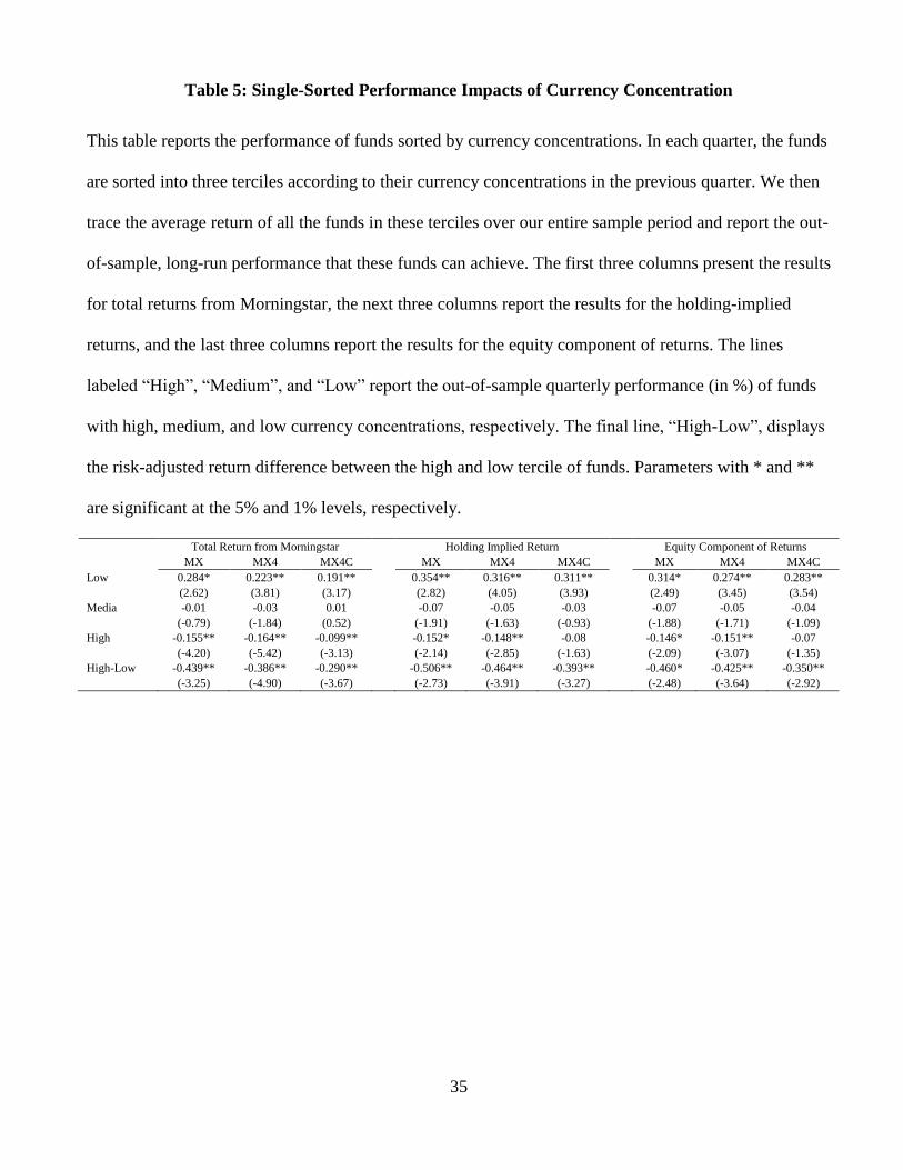
The results show a strong and statistically significant negative relationship between currency
concentration and fund performance. The economic impact of the currency concentration policy
(computed in the same way as in Table 3) is approximately 176, 154, and 116 basis points per year for
total returns and 202, 186, and 157 basis points per year for holding-based performance in the case of
the MX-, MX4-, and MX4C-adjusted returns, respectively.
[Insert Table 5 here]
Figure 1 visualizes the return and alpha time series that are generated by funds with high and low
currency concentrations. In particular, each quarter, the funds are sorted into three terciles according to
their currency concentrations. We then plot the accumulated fund performance for high- and low-tercile
funds. To save space, we only depict the total return-based performance (MX, MX4, and MX4C) here;

18
refer to the Internet Appendix for the holding-based performance plots. If low-currency-concentration
funds outperform high-currency-concentration funds, as reported in Table 5, we would expect the
performance gap between the two types of funds to increase (and become wider) over time. The figure
clearly shows such a pattern, which further confirms the underperformance of high-concentration funds.
[Insert Figure 1 here]
C. Multivariate Analysis
We now consider a multivariate analysis. We relate out-of-sample fund performance to funds’ currency
policies and a set of fund-level control variables in quarterly Fama-MacBeth regressions and report the
results in Table 6.
In Panel A, the dependent variable is quarterly fund total returns (in percentage) adjusted by the
three nested models. The difference between Models 1-3 and Models 4-6 is that Models 1-3 control for
local currency weight and fund characteristics, including fees, turnover, age, and TNA, whereas Models
4-6 further control for the characteristics of the equity holdings of funds, including the number of stocks,
the industry concentration, and the degree of concentration in domestic and foreign stocks. For each
model, Panel A tabulates the time-series averages of the cross-sectional parameters and their Newey-
West t-statistics with 5 lags (to control for the potential seasonality in quarterly regressions; our results
are robust to the choice of lags). In Panel B, we report similar statistics for the risk-adjusted, holding-
implied returns. To save space, however, we only tabulate the coefficients for the main variables in
Panel B (and in later tables). The full specifications of the regression parameters can be found in the
Internet Appendix.
The results are consistent with the previous portfolio analyses and show a strong and significant
correlation between currency policies and fund returns. In Models 4-6, a one-standard-deviation increase
in currency concentration is related to a total return performance that is 137, 123, and 103 basis points
lower and a holding-based performance that is 155, 141, and 117 basis points lower for MX-, MX4-, and

19
MX4C-adjusted returns, respectively.10
Hence, the negative performance impact of currency
concentration is not only statistically significant but also economically relevant.
[Insert Table 6 here]
Further, we conduct a series of additional analyses related to the negative performance impact of
currency concentration. We first plot, in Figure 2, the time series variation of the quarterly Fama-
MacBeth regression coefficients of currency concentration from Models 4-6 of Panel A. From the plots,
the performance impact of currency concentration is generally negative. One notable exception occurs in
the third and fourth quarters of 2008, during which concerns regarding the global financial crisis may
dominate currency considerations. Nonetheless, the overall impact of currency concentration is clearly
negative in most quarters across all the performance measures.
[Insert Figure 2 here]
Next, because the majority of the funds are US domiciled, we also conduct robustness checks to
explore whether the impact of currency policy arises from US funds only. Panels C and D of Table 6,
therefore, apply the previous analyses of Panels A and B to the subsamples of US and non-US funds,
respectively. To save space, we only tabulate side by side the subsample regression coefficients
corresponding to those from Models 4-6 of Panels A and B—the first three columns for US funds and
the next three columns for non-US funds. Subsample regressions based on Models 1-3 of Panels A and
B yield similar conclusions. The results show that the performance impact of currency concentration
prevails in both US and non-US funds, although the magnitude of the performance impact is greater for
US funds.
Finally, Table 7 explores the general impact of currency concentration on equity performance. The
layout is similar to that of Panel B, Table 6, except that we focus on the equity component of holding-
implied returns rather than holding-implied returns. The results are consistent with the previous results
10The quarterly economic magnitude is estimated as the one-standard-deviation change in currency concentration times the regression
coefficient. We further annualize this impact by multiplying its value by four.

20
and show that a strong negative relationship exists between equity performance and currency
concentration. A one-standard-deviation increase in currency concentration is related to a reduction in
MX-, MX4-, and MX4C-adjusted equity performance of 131, 120, and 108 basis points, respectively.
The magnitude of the impact is on par with that reported in Table 6, confirming that the performance
impact of ICVR is mainly achieved through the equity channel.
[Insert Table 7 here]
In addition to these analyses, we also find that the negative correlation between performance and
currency policies is robust when we use panel specifications and when we control for family or style
affiliations. The Internet Appendix provides the details of these analyses.
V. Currency Risk, Hedging Policies, and Performance
We can now combine the different pieces of the analyses and provide an integrated view. We have
shown that currency risk affects portfolio performance (Section III). We have identified one main
operational hedging policy (i.e., currency concentration) that has been used to manage such risk, and we
have demonstrated that this policy reduces fund performance in general and equity performance in
particular (Section IV). We can now determine whether this policy provides an important channel
through which currency risk negatively affects fund performance.
More specifically, using a two-stage specification, we can project currency concentration on ICVR
and focus on the predicted component to examine the extent to which the impact of currency risk on
performance is specifically channeled through currency concentration. As a “Placebo” test, we also
perform the same projection based on cultural distance—the proxy that has the second largest
explanatory power (after ICVR) in Table 3. Hence, we project currency concentration on ICVR and
cultural distance to decompose currency concentration into components due to ICVR, cultural distance,
and other factors (the residual). Then, we investigate which components have the explanatory power for
fund performance.

21
We report the out-of-sample performance impact of various components of currency policies in
Table 8. Panel A focuses on total returns, while Panel B focuses on holding-based returns. In each panel,
the fund performance is again adjusted by using MX in Models 1 and 4, MX4 in Models 2 and 5, and
MX4C in Models 3 and 6. In the case of total returns, our main finding is that a one-standard-deviation
increase in ICVR-induced concentration can reduce fund total return performance by 33, 28, and 22
basis points per year and holding-implied return performance by 41, 32, and 29 basis points per year for
MX-, MX4-, and MX4C-adjusted returns, respectively. These results not only are statistically significant
but also explain a significant proportion of the total impact of ICVR on fund performance, as
documented in Table 3. By contrast, the “Placebo” test suggests that distance does not affect fund
performance through the channel of currency concentration. This result is logical because distance, if it
is related to superior equity information, should mostly affect performance through equity policies, not
currency policies.
[Insert Table 8 here]
In addition to ICVR, the residual also absorbs a quite significant proportion of negative fund
performance through the channel of currency concentration. This result is not surprising for two reasons.
First, we only projected a linear impact of ICVR on currency concentration. Any nonlinear effect could
be captured by the residual. Hence, we do not expect the linearly projected currency policy to fully
explain the return impact of ICVR. Second, ICVR, while important, is only one type of currency risk
that may incentivize operational hedging. Other types of currency risk, such as catastrophic risk (e.g.,
Burnside, Eichenbaum, Kleshchelski, and Rebelo (2011)), and exogenous characteristics may also
constrain currency concentration. The overall results, however, clearly demonstrate that the policy
adopted to address currency risk is highly responsible for the impact of currency risk on performance.
Finally, we also decompose the equity performance impact of currency concentration into the impact
related to currency risk and the other possible explanations and report the results in Panel C of Table 8.
The results show that the ICVR-related component of currency concentration is strongly related to the
22
equity component of performance. In particular, a one-standard-deviation change is related to a
reduction in MX-, MX4- and MX4C-adjusted equity performance of 37, 27, and 24 basis points,
respectively. Again, the economic magnitude is on par with that reported in the previous two panels,
confirming that currency risk mainly affects equity returns through the policy of currency concentration.
In addition, the “Placebo” test on cultural distance fails to detect a significant impact through this
channel.
Overall, these results show that the need to concentrate on a limited number of currencies directly
affects fund performance. This effect is sizable and is mainly achieved through the equity portion of the
portfolio. That is, the currency policy conditions the choice of stocks in a suboptimal manner and
reduces fund performance.
VI. Conclusion
We study the determinants of currency management in international equity funds and their implications
for fund performance. To rationalize the surprising finding that currency risk reduces equity
performance, we hypothesize that the combination of base currency and style affiliation creates
constraints for international funds. To be more specific, funds with highly embedded currency risk from
their benchmarks tend to invest in markets with less volatile currencies, leading to a currency
concentration in portfolio holdings. However, this currency concentration departs from the optimal
equity allocation strategy across countries and may reduce fund performance.
We test this hypothesis by using a worldwide sample of mutual funds. We show that higher
embedded currency risk (ICVR) leads to higher currency concentration and that higher currency
concentration is typically related to lower fund performance. Furthermore, we confirm that currency risk
can lead to lower equity performance through the channel of currency concentration.
Overall, we document that the effect of currency risk and a management policy of currency
concentration is not limited to the currency market. Rather, it extends to the equity market and affects

23
the equity choice/performance of international funds. These results shed initial light on the complicated
determinants of currency management for international mutual funds and their implications for fund
performance.
24
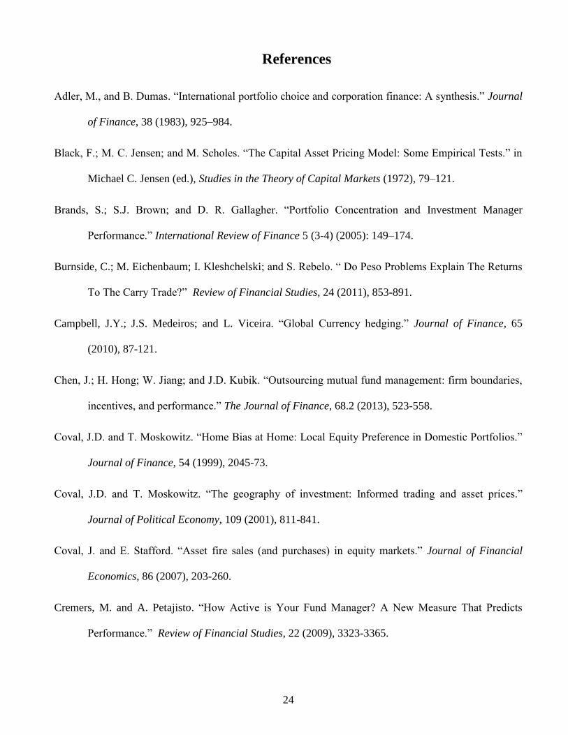
References
Adler, M., and B. Dumas. “International portfolio choice and corporation finance: A synthesis.” Journal
of Finance, 38 (1983), 925–984.
Black, F.; M. C. Jensen; and M. Scholes. “The Capital Asset Pricing Model: Some Empirical Tests.” in
Michael C. Jensen (ed.), Studies in the Theory of Capital Markets (1972), 79–121.
Brands, S.; S.J. Brown; and D. R. Gallagher. “Portfolio Concentration and Investment Manager
Performance.” International Review of Finance 5 (3-4) (2005): 149–174.
Burnside, C.; M. Eichenbaum; I. Kleshchelski; and S. Rebelo. “ Do Peso Problems Explain The Returns
To The Carry Trade?” Review of Financial Studies, 24 (2011), 853-891.
Campbell, J.Y.; J.S. Medeiros; and L. Viceira. “Global Currency hedging.” Journal of Finance, 65
(2010), 87-121.
Chen, J.; H. Hong; W. Jiang; and J.D. Kubik. “Outsourcing mutual fund management: firm boundaries,
incentives, and performance.” The Journal of Finance, 68.2 (2013), 523-558.
Coval, J.D. and T. Moskowitz. “Home Bias at Home: Local Equity Preference in Domestic Portfolios.”
Journal of Finance, 54 (1999), 2045-73.
Coval, J.D. and T. Moskowitz. “The geography of investment: Informed trading and asset prices.”
Journal of Political Economy, 109 (2001), 811-841.
Coval, J. and E. Stafford. “Asset fire sales (and purchases) in equity markets.” Journal of Financial
Economics, 86 (2007), 203-260.
Cremers, M. and A. Petajisto. “How Active is Your Fund Manager? A New Measure That Predicts
Performance.” Review of Financial Studies, 22 (2009), 3323-3365.

25
Dahlquist, M., and G. Robertsson. "Direct Foreign Ownership, Institutional Investors, and Firm
Characteristics." Journal of Financial Economics, 59 (2001), 413-440.
Dumas, B., and B. Solnik. “The world price of foreign exchange risk”, Journal of Finance, 50 (1995),
445–479.
Eugene, F. “Forward and spot exchange rates.” Journal of Monetary Economics, 14 (1984), 319–338.
Fama, E. F., and K. R. French. “The Cross Section of Expected Stock Returns.” Journal of Finance, 47
(1992), 427–65.
Fama, E. F., and K. R. French. “Size, Value, and Momentum in International Stock Returns.” Journal of
Financial Economics, 105 (2012), 457-472.
Ferreira, M. A.; A. Keswani; A. F. Miguel; and S. B. Ramos. “The determinants of mutual fund
performance: A cross-country study”. Review of Finance, 17.2 (2013), 483-525.
Ferson, W. E., and R. W. Schadt. “Measuring fund strategy and performance in changing economic
conditions.” Journal of Finance, 51 (1996), 425-461.
Froot, K. A.; P. G. J. O’Connell; and M. S. Seasholes. “The Portfolio Flows of International Investors.”
Journal of Financial Economics, 59 (2001), 151–93.
Fung, W. and D. A. Hsieh. “Hedge fund benchmarks: A risk based approach.” Financial Analysts
Journal, 60 (2004), 65–80.
Griffin, J. M. “Are the Fama and French Factors Global or Country Specific?” Review of Financial
Studies, 15 (2002), 783-803.
Harvey, C. R. “The world price of covariance risk.” Journal of Finance, 46 (1991), 111-157.
Huang, J.C.; C. Sialm; and H. Zhang, "Risk shifting and mutual fund performance." Review of Financial
Studies, 24.8 (2011), 2575-2616.

26
Kacperczyk, M. and A. Seru. “Fund Manager Use of Public Information.” Journal of Finance, 52.2
(2007), 485-528.
Kacperczyk, M.T., C. Sialm, and L. Zheng. “On Industry Concentration of Actively Managed Equity
Mutual Funds.” Journal of Finance, 60 (2005), 1983-2011.
Kang, J-K., and R. M. Stulz. “Why is there a Home Bias? An Analysis of Foreign Portfolio Equity
Ownership in Japan.” Journal of Financial Economics, 46 (1997), 2–18.
Lettau, M., and S. Ludvigson. “Resurrecting the (C) CAPM: A cross-sectional test when risk premia are
time-varying.” Journal of Political Economy, 109 (2001), 1238-87.
Levich R., G Hayt, B. Prpston. “1998 Survey of Derivatives and Risk management Practices by U.S.
Institutional Investors.” Working paper, (1998).
Lustig, H.; N. Roussanov; and A. Verdelhan. “Common risk factors in currency markets.” Review of
Financial Studies, 24.11 (2011), 3731-3777.
Sarkissian S and MJ. Schill. “The overseas listing decision: New evidence of proximity preference.”
Review of Financial Studies, 17 (2004), 769-809.
Shleifer, A., and R. Vishny. “The limits of arbitrage.” Journal of Finance, 52 (1997), 35-55.
Solnik, B. “The international pricing of risk: An empirical investigation of the world capital market
structure.” Journal of Finance, 29 (1974), 48-54.
27
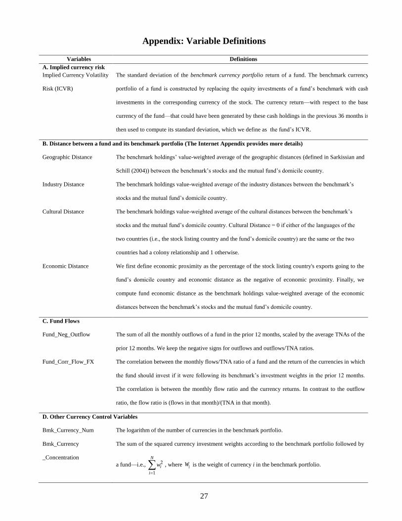
Appendix: Variable Definitions
Variables Definitions
A. Implied currency risk
Implied Currency Volatility
Risk (ICVR)
The standard deviation of the benchmark currency portfolio return of a fund. The benchmark currency
portfolio of a fund is constructed by replacing the equity investments of a fund’s benchmark with cash
investments in the corresponding currency of the stock. The currency return—with respect to the base
currency of the fund—that could have been generated by these cash holdings in the previous 36 months is
then used to compute its standard deviation, which we define as the fund’s ICVR.
B. Distance between a fund and its benchmark portfolio (The Internet Appendix provides more details)
Geographic Distance The benchmark holdings’ value-weighted average of the geographic distances (defined in Sarkissian and
Schill (2004)) between the benchmark’s stocks and the mutual fund’s domicile country.
Industry Distance The benchmark holdings value-weighted average of the industry distances between the benchmark’s
stocks and the mutual fund’s domicile country.
Cultural Distance The benchmark holdings value-weighted average of the cultural distances between the benchmark’s
stocks and the mutual fund’s domicile country. Cultural Distance = 0 if either of the languages of the
two countries (i.e., the stock listing country and the fund’s domicile country) are the same or the two
countries had a colony relationship and 1 otherwise.
Economic Distance We first define economic proximity as the percentage of the stock listing country's exports going to the
fund’s domicile country and economic distance as the negative of economic proximity. Finally, we
compute fund economic distance as the benchmark holdings value-weighted average of the economic
distances between the benchmark’s stocks and the mutual fund’s domicile country.
C. Fund Flows
Fund_Neg_Outflow The sum of all the monthly outflows of a fund in the prior 12 months, scaled by the average TNAs of the
prior 12 months. We keep the negative signs for outflows and outflows/TNA ratios.
Fund_Corr_Flow_FX The correlation between the monthly flows/TNA ratio of a fund and the return of the currencies in which
the fund should invest if it were following its benchmark’s investment weights in the prior 12 months.
The correlation is between the monthly flow ratio and the currency returns. In contrast to the outflow
ratio, the flow ratio is (flows in that month)/(TNA in that month).
D. Other Currency Control Variables
Bmk_Currency_Num The logarithm of the number of currencies in the benchmark portfolio.
Bmk_Currency
_Concentration
The sum of the squared currency investment weights according to the benchmark portfolio followed by
a fund—i.e.,
N
i
i
w
2
1
, where iw is the weight of currency i in the benchmark portfolio.

28
E. Fund Characteristics
Fund_FEE The lagged annual expense ratio as reported in Morningstar.
Fund_Turnover The lagged annual turnover ratio as reported in Morningstar.
Fund_AGE Log of the number of operational years since inception; one-period lagged.
Fund_TNA Log of portfolio TNAs in US dollars; one-period lagged.
F. Fund Equity Management
Stock_Num The logarithm of the number of stocks in a portfolio.
Stock_Concentration_Dom Stock_Concentration_Dom = i
iw
2
Domestic Stock, where iw
is the investment weight of domestic
security in a given portfolio based on the most updated holdings information for a portfolio.
Stock_Concentration_Fore Stock_Concentration_Dom = i
iw
2
Foreign Stock, where iw
is the investment weight of foreign
security in a given portfolio based on the most updated holdings information for a portfolio.
Industry Concentration ∑ ∑
, where is the investment of the fund in sector and
is the investment weight of the benchmark portfolio in sector .
G. Performance Measures and Factors
Fund Total Returns Fund return as reported by Morningstar. For multiple share classes, fund total return is computed as the
TNA-weighted return of all share classes of the portfolio, where TNA values are one-month lagged.
Holding-Implied Returns Monthly portfolio return computed based on the most updated quarterly holdings information.
The Equity Component
of Fund Returns
The equity component of fund returns is the hypothetical equity return that the portfolio would have had
if the FX returns were removed, i.e., , 1 ,(1 r )Fund
n t n tn , where , 1
Fund
n t is the investment weights of the
fund in stock n, ,rn t
is the return of the stock in its local currency.
Fund Performance or Risk-
adjusted Returns
Risk-adjusted returns are defined as fund returns less the productions between its factor betas multiplied
by the realized factor values in a given month, i.e., , ,f t f t tr X , where ,f tr is the return of fund f
in month t, tX is the realized factor return in the sample month, and is the factor loading of the fund
estimated over the whole sample period.
H. Currency Policies (Currency policies are defined relative to their benchmark)
Local Currency Weight
Benchmark-adjusted, base-currency investment weight. It is computed as the base-currency investment
weight of a fund less the corresponding weight of its benchmark.
Currency Concentration Benchmark-adjusted currency concentration. It is computed as the sum of the squared currency weights
less the sum implied by its benchmark.

29
Table 1: Summary Statistics of International Mutual Funds
This table presents the summary statistics on how mutual funds invest in foreign assets and currencies.
In Panel A, the first two columns report the number of fund domicile countries and mutual funds by year,
followed by a column to summarize the TNAs of these funds in trillions of US dollars. Only funds with
a valid benchmark are included. The next three columns show the number of mutual funds with foreign
equity less than 20%, between 20% and 50%, or larger than 50% of their overall equity holdings (in
terms of US dollar value). The last three columns report the number of funds that hold 1, between 2 and
8, and more than 8 foreign currencies of stocks in their holdings portfolio. Foreign equity is defined as
stocks that are not listed in a fund’s domicile country. Foreign currencies are defined as currencies that
are not the base currency of a fund. Panel B reports the number of funds by countries and years.
Panel A: International Mutual Funds
Year # Countries # of Funds Total TNA # of Benchmarked Funds with # of Benchmarked Funds
with valid (Trillion US Dollar) Specified Foreign Holdings with # foreign currencies
Benchmark <20% 20%-50% 50%-100% 1 (1, 8] >8
2001 19 2598 2.48949 1874 127 597 368 1628 305
2002 20 3339 2.36954 2230 228 881 478 2015 376
2003 27 3960 1.93271 2504 294 1162 611 2215 405
2004 27 4385 2.81036 2725 361 1299 642 2434 569
2005 27 4614 3.15467 2878 366 1370 609 2513 630
2006 27 5007 3.86576 3025 446 1536 667 2637 788
2007 28 5140 4.4925 3099 456 1585 641 2728 852
2008 30 5164 4.28128 3072 478 1614 573 2763 968
2009 30 4943 2.44582 2989 464 1490 566 2615 879
2010 30 4462 3.46004 2677 432 1353 470 2355 856
2011 28 4282 4.1656 2504 417 1361 419 2318 857
2012 26 3543 3.64726 2227 320 996 359 1950 694

30
2001 2002 2003 2004 2005 2006 2007 2008 2009 2010 2011 2012
United States 2065 2217 2277 2368 2458 2598 2669 2656 2537 2355 2223 2096
United Kingdom 165 219 298 351 375 444 449 466 441 405 418 242
Luxembourg 99 249 335 406 432 480 493 514 468 408 361 209
France 10 63 133 204 233 265 283 316 323 269 239 202
Germany 56 152 206 208 210 217 214 208 181 166 155 142
India 0 0 1 62 87 141 141 135 147 144 141 112
Spain 7 67 102 111 118 120 125 120 114 100 89 83
Sweden 24 54 87 91 87 97 98 97 96 18 83 79
Switzerland 38 35 56 61 64 67 81 72 71 67 84 78
Belgium 43 66 80 88 88 94 92 81 76 69 55 47
Norway 20 30 42 48 52 51 52 53 49 47 46 46
Denmark 15 42 82 85 93 93 96 107 100 98 90 42
Austria 13 29 38 42 42 46 45 45 43 40 42 40
Ireland 16 44 82 91 100 101 94 106 112 98 95 40
Finland 6 15 28 32 37 41 47 47 41 42 40 23
Netherlands 10 18 35 37 38 39 36 32 31 29 27 23
Liechtenstein 0 0 20 27 28 29 33 31 31 31 28 11
Guernsey 7 10 10 9 10 10 9 8 8 7 7 7
Italy 1 22 29 32 32 34 32 13 15 14 10 6
Cayman Islands 0 0 1 5 4 4 6 4 4 4 4 4
Jersey 0 2 3 3 3 3 3 6 6 6 7 3
Portugal 0 3 4 4 4 4 4 4 4 3 3 3
British Virgin Islands 2 2 2 3 1 2 3 2 2 2 2 2
Channel Islands 0 0 0 0 0 0 0 1 1 1 0 1
Malaysia 0 0 1 8 10 19 24 30 29 31 26 1
Taiwan 0 0 0 0 0 0 0 0 0 1 1 1
Andorra 0 0 0 0 0 3 3 0 6 0 0 0
Bermuda 1 0 2 3 2 2 2 2 2 2 2 0
Greece 0 0 4 4 4 0 3 3 1 1 0 0
Hong Kong 0 0 0 0 0 0 0 1 1 1 1 0
Isle of Man 0 0 2 2 2 3 3 3 3 3 3 0
Singapore 0 0 0 0 0 0 0 1 0 0 0 0
Total 2598 3339 3960 4385 4614 5007 5140 5164 4943 4462 4282 3543
Panel B: Mutual Funds with Valid Benchmark by Countries
31
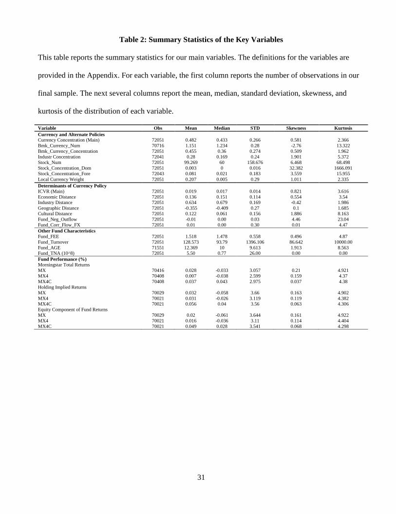
Table 2: Summary Statistics of the Key Variables
This table reports the summary statistics for our main variables. The definitions for the variables are
provided in the Appendix. For each variable, the first column reports the number of observations in our
final sample. The next several columns report the mean, median, standard deviation, skewness, and
kurtosis of the distribution of each variable.
Variable Obs Mean Median STD Skewness Kurtosis
Currency and Alternate Policies Currency Concentration (Main) 72051 0.482 0.433 0.266 0.581 2.366
Bmk_Currency_Num 70716 1.151 1.234 0.28 -2.76 13.322
Bmk_Currency_Concentration 72051 0.455 0.36 0.274 0.509 1.962
Industr Concentration 72041 0.28 0.169 0.24 1.901 5.372
Stock_Num 72051 99.269 60 158.676 6.468 68.498
Stock_Concentration_Dom 72051 0.003 0 0.016 32.382 1666.091
Stock_Concentration_Fore 72043 0.081 0.021 0.183 3.559 15.955
Local Currency Weight 72051 0.207 0.005 0.29 1.011 2.335
Determinants of Currency Policy
ICVR (Main) 72051 0.019 0.017 0.014 0.821 3.616
Economic Distance 72051 0.136 0.151 0.114 0.554 3.54 Industry Distance 72051 0.634 0.679 0.169 -0.42 1.986
Geographic Distance 72051 -0.355 -0.409 0.27 0.1 1.685
Cultural Distance 72051 0.122 0.061 0.156 1.886 8.163
Fund_Neg_Outflow 72051 -0.01 0.00 0.03 4.46 23.04
Fund_Corr_Flow_FX 72051 0.01 0.00 0.30 0.01 4.47
Other Fund Characteristics
Fund_FEE 72051 1.518 1.478 0.558 0.496 4.87
Fund_Turnover 72051 128.573 93.79 1396.106 86.642 10000.00
Fund_AGE 71551 12.369 10 9.613 1.913 8.563 Fund_TNA (10^8) 72051 5.50 0.77 26.00 0.00 0.00
Fund Performance (%)
Morningstar Total Returns
MX 70416 0.028 -0.033 3.057 0.21 4.921
MX4 70408 0.007 -0.038 2.599 0.159 4.37
MX4C 70408 0.037 0.043 2.975 0.037 4.38
Holding Implied Returns
MX 70029 0.032 -0.058 3.66 0.163 4.902
MX4 70021 0.031 -0.026 3.119 0.119 4.382 MX4C 70021 0.056 0.04 3.56 0.063 4.306
Equity Component of Fund Returns
MX 70029 0.02 -0.061 3.644 0.161 4.922
MX4 70021 0.016 -0.036 3.11 0.114 4.404
MX4C 70021 0.049 0.028 3.541 0.068 4.298

32
Table 3: Performance Impacts of Currency Risks
This table reports the out-of-sample performance of funds sorted by their ICVR. In each quarter, funds
are sorted into three terciles according to their ICVR in the previous quarter. We then trace the average
return of all the funds in these terciles over our entire sample period and report the out-of-sample, long-
run performance that these funds can achieve. The first three columns present the results for total returns
from Morningstar, the next three columns report the results for the holding-implied returns, and the last
three columns report the results for the equity component of returns. In each block, MX adjusts fund
performance by the traditional ICAPM, MX4 adds the Fama-French-Carhart four factors in the domestic
market to the ICAPM, and MX4C includes the Lustig et al. (2011) carry-trade factor on top of the MX4
adjustment. The lines labeled “High”, “Medium”, and “Low” report the out-of-sample quarterly
performance (in %) of funds with high, medium, and low ICVR, respectively. The final line, “High-
Low”, displays the risk-adjusted return difference between the high and low tercile of funds. Parameters
with * and ** are significant at the 5% and 1% levels, respectively.
Total Return from Morningstar Holding Implied Return Equity Component of Returns
MX MX4 MX4C MX MX4 MX4C MX MX4 MX4C
Low 0.174* 0.164** 0.138** 0.16 0.174** 0.163** 0.14 0.141* 0.137*
(2.55) (4.18) (3.41) (1.82) (3.22) (3.04) (1.57) (2.51) (2.48)
Media 0.02 -0.01 0.045* 0.03 0.01 0.06 0.02 0.00 0.068*
(0.78) (-0.72) (2.21) (0.94) (0.35) (1.96) (0.73) (0.04) (2.28)
High -0.086* -0.138** -0.091** -0.089** -0.091** -0.056* -0.091** -0.094** -0.063*
(-2.44) (-4.50) (-2.92) (-2.94) (-3.39) (-2.03) (-3.09) (-3.64) (-2.46)
High-Low -0.260** -0.301** -0.229** -0.247* -0.266** -0.219** -0.227* -0.235** -0.200**
(-3.20) (-5.71) (-4.29) (-2.52) (-4.38) (-3.70) (-2.35) (-3.91) (-3.46)
33
Table 4: The Formation of Currency Policies (First Stage Regressions)
This table presents the results of the first-stage regressions between currency policies and proxies for
information, flow uncertainty, and currency risk,
, where is the currency
concentration of fund in quarter t+1, ICVR is the measure of currency volatility risk, Dist is one of the
four proxies for distance between the fund and its benchmark stocks, and FlowUnc is the proxy for flow
uncertainty. The vector X stacks all the control variables, including the fund’s fees, age, TNA, turnover,
industry concentration, and degree of concentration in domestic and foreign stocks, as well as the
number of stocks in each fund’s portfolio. We also include the benchmarked currency member
(Bmk_Currency_Num) and currency concentration (Bmk_Currency_Concentration). Parameters with *
and ** are significant at the 5% and 1% levels, respectively.

34
Fama Macbeth Regression Pooled Panel Regression
Model1 Model2 Model3 Model4 Model5 Model6 Model7 Model8
A. Implied Currency Risk
ICVR 3.895** 2.373** 4.115** 3.105** 3.786** 2.292** 3.880** 2.861**
(15.49) (11.74) (15.76) (12.44) (15.80) (8.41) (17.73) (10.81)
B. Fund Distance
Economic Distance 0.085** -0.006 0.101** 0.013
(5.30) (-0.31) (2.80) (0.39)
Industry Distance 0.088** 0.057** 0.086** 0.060*
(7.99) (10.58) (3.17) (2.36)
Geographic Distance 0.082** 0.029** 0.080** 0.031*
(19.03) (8.02) (5.49) (2.25)
Cultural Distance 0.222** 0.168** 0.220** 0.171**
(12.43) (11.94) (6.64) (5.51)
C. Fund Flow Uncertainty
Fund_Neg_Outflow -0.003 -0.002 0.000 0.000
(-0.79) (-0.48) (0.53) (0.19)
Fund_Corr_Flow_FX -0.011** -0.009** -0.013** -0.011**
(-3.68) (-3.21) (-4.53) (-3.75)
D. Currency Control Variables
Bmk_Currency_Num -0.001** -0.000** -0.001** -0.000*
(-8.96) (-5.10) (-4.13) (-2.13)
Bmk_Currency_Concentration -0.202** -0.179** -0.199** -0.173**
(-36.49) (-28.66) (-18.77) (-15.97)
E. Fund Characteristics Control Variables
Fund_FEE -0.005 0.000 0.002 0.005 -0.006 0.000 0.001 0.005
(-1.94) (-0.12) (0.74) (1.92) (-1.18) (-0.08) (0.20) (0.95)
Fund_Turnover 0.002 0.003 0.002 0.003 0.001 0.002 0.002 0.002
(0.96) (1.75) (1.62) (1.80) (0.39) (1.04) (0.89) (1.05)
Fund_AGE 0.005** 0.005** 0.008** 0.007** 0.006 0.005 0.008* 0.006*
(4.18) (3.72) (7.60) (6.45) (1.67) (1.44) (2.37) (2.06)
Fund_TNA -0.003* -0.002 -0.004** -0.003** -0.004** -0.003* -0.005** -0.004**
(-2.59) (-1.95) (-5.04) (-4.38) (-2.58) (-1.97) (-3.32) (-2.59)
F. Fund Equity Management Control Variables
Industry Concentration -0.221** -0.196** -0.166** -0.154** -0.202** -0.180** -0.155** -0.145**
(-9.96) (-8.92) (-9.38) (-8.56) (-6.15) (-5.82) (-5.73) (-5.45)
Stock_Num 0.019** 0.019** 0.015** 0.016** 0.020** 0.022** 0.017** 0.018**
(10.37) (9.59) (7.18) (7.37) (5.21) (5.64) (4.75) (5.08)
Stock_Concentration_Dom 2.283** 2.122** 1.237** 1.325** 1.803** 1.725** 1.085** 1.197**
(8.95) (9.63) (9.07) (9.86) (7.41) (7.42) (6.36) (6.52)
Stock_Concentration_Fore 0.861** 0.845** 0.816** 0.810** 0.845** 0.834** 0.808** 0.805**
(25.30) (25.25) (26.53) (26.73) (27.21) (27.53) (29.37) (29.06)
Constant -0.111** -0.018* -0.005 0.041** -0.113** -0.019 -0.004 0.043**
(-23.06) (-2.59) (-0.85) (6.67) (-20.51) (-1.33) (-0.41) (2.89)
Observations 69,931 69,931 69,931 69,931 69,931 69,931 69,931 69,931
R-squared 0.319 0.366 0.411 0.429 0.305 0.354 0.396 0.415
35
Table 5: Single-Sorted Performance Impacts of Currency Concentration
This table reports the performance of funds sorted by currency concentrations. In each quarter, the funds
are sorted into three terciles according to their currency concentrations in the previous quarter. We then
trace the average return of all the funds in these terciles over our entire sample period and report the out-
of-sample, long-run performance that these funds can achieve. The first three columns present the results
for total returns from Morningstar, the next three columns report the results for the holding-implied
returns, and the last three columns report the results for the equity component of returns. The lines
labeled “High”, “Medium”, and “Low” report the out-of-sample quarterly performance (in %) of funds
with high, medium, and low currency concentrations, respectively. The final line, “High-Low”, displays
the risk-adjusted return difference between the high and low tercile of funds. Parameters with * and **
are significant at the 5% and 1% levels, respectively.
Total Return from Morningstar Holding Implied Return Equity Component of Returns
MX MX4 MX4C MX MX4 MX4C MX MX4 MX4C
Low 0.284* 0.223** 0.191** 0.354** 0.316** 0.311** 0.314* 0.274** 0.283**
(2.62) (3.81) (3.17) (2.82) (4.05) (3.93) (2.49) (3.45) (3.54)
Media -0.01 -0.03 0.01 -0.07 -0.05 -0.03 -0.07 -0.05 -0.04
(-0.79) (-1.84) (0.52) (-1.91) (-1.63) (-0.93) (-1.88) (-1.71) (-1.09)
High -0.155** -0.164** -0.099** -0.152* -0.148** -0.08 -0.146* -0.151** -0.07
(-4.20) (-5.42) (-3.13) (-2.14) (-2.85) (-1.63) (-2.09) (-3.07) (-1.35)
High-Low -0.439** -0.386** -0.290** -0.506** -0.464** -0.393** -0.460* -0.425** -0.350**
(-3.25) (-4.90) (-3.67) (-2.73) (-3.91) (-3.27) (-2.48) (-3.64) (-2.92)

36
Table 6: Performance Impacts of Currency Concentration in Fama-MacBeth Regressions
This table reports the performance impact of currency concentration according to Fama-MacBeth
regressions. In Panel A, we regress MX-, MX4-, and MX4C-adjusted quarterly Morningstar total returns
(in %) of the funds on the lagged currency concentration and the lagged control variables and tabulate
the time-series averages of the cross-sectional parameters as well as their Newey-West t-statistics with 5
lags. Panel B reports the result of the holding-implied returns. Panels C and D report the results of
similar tests using the US and non-US subsamples for the Morningstar total returns and holding-implied
returns, respectively. Parameters with * and ** are significant at the 5% and 1% levels, respectively.
Panel A: Total Returns from Morningstar
Model1 Model2 Model3 Model4 Model5 Model6
MX MX4 MX4C MX MX4 MX4C
Currency Concentration -1.169** -1.061** -0.802** -1.292** -1.156** -0.968**
(-3.26) (-5.44) (-3.25) (-3.30) (-6.02) (-4.29)
Local Currency Weight 0.097 0.107 -0.086 -0.027 0.016 -0.167
(1.39) (1.32) (-0.88) (-0.32) (0.17) (-1.62)
Fund_FEE -0.100 -0.136* -0.242** -0.133* -0.158** -0.262**
(-1.61) (-2.50) (-3.39) (-2.50) (-3.28) (-4.31)
Fund_Turnover -0.048 -0.057* -0.126** -0.045 -0.054* -0.118**
(-1.71) (-2.52) (-7.02) (-1.67) (-2.41) (-6.72)
Fund_AGE 0.067 0.047* 0.059 0.054 0.040 0.048
(1.91) (2.10) (2.00) (1.85) (1.94) (1.91)
Fund_TNA -0.023 -0.003 -0.018 -0.001 0.011 -0.001
(-0.81) (-0.17) (-1.21) (-0.05) (0.66) (-0.06)
Bmk_Currency_Concentration 0.031 0.126 0.029 -0.064 0.044 -0.077
(0.47) (1.59) (0.43) (-0.92) (0.52) (-1.01)
Stock_Num 0.829 0.864* 1.111**
(1.97) (2.60) (2.90)
Industry Concentration -0.056** -0.018 0.013
(-2.98) (-1.27) (0.69)
Stock_Concentration_Dom 4.287 2.759 2.388*
(1.76) (1.36) (2.21)
Stock_Concentration_Fore 0.375 0.348 0.766*
(0.73) (1.21) (2.03)
Constant -0.027 -0.095** -0.027 0.000 -0.074* -0.001
(-1.02) (-3.11) (-1.01) (-0.02) (-2.47) (-0.03)
Observations 69,923 69,915 69,915 69,908 69,900 69,900
R-squared 0.033 0.024 0.019 0.052 0.04 0.034
F 3.23 7.28 11.11 3.70 6.28 9.75
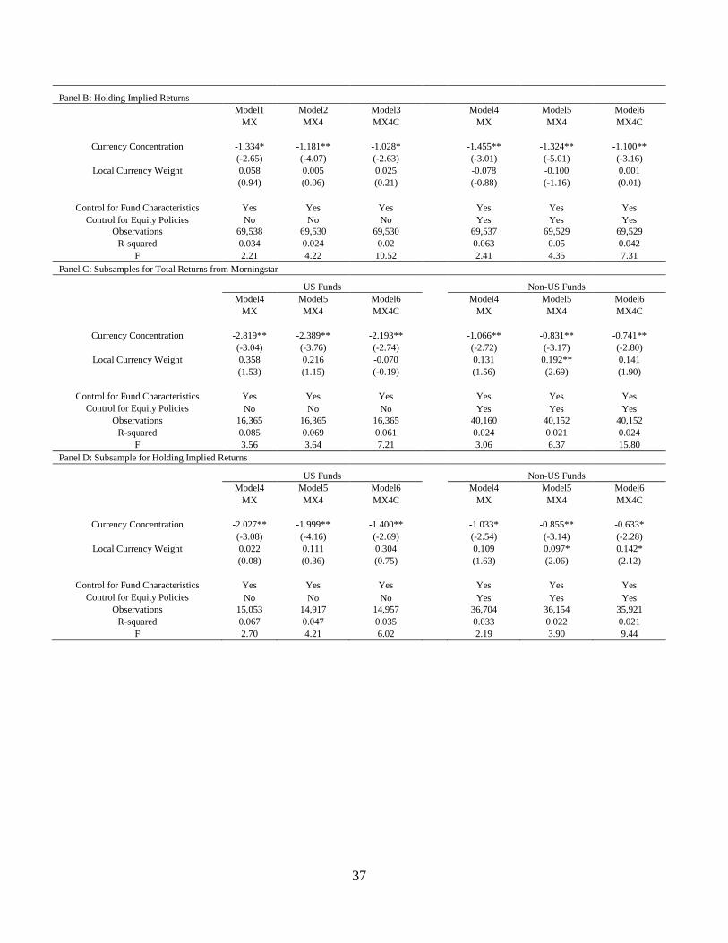
37
Panel B: Holding Implied Returns Model1 Model2 Model3 Model4 Model5 Model6
MX MX4 MX4C MX MX4 MX4C
Currency Concentration -1.334* -1.181** -1.028* -1.455** -1.324** -1.100**
(-2.65) (-4.07) (-2.63) (-3.01) (-5.01) (-3.16)
Local Currency Weight 0.058 0.005 0.025 -0.078 -0.100 0.001
(0.94) (0.06) (0.21) (-0.88) (-1.16) (0.01)
Control for Fund Characteristics Yes Yes Yes Yes Yes Yes
Control for Equity Policies No No No Yes Yes Yes
Observations 69,538 69,530 69,530 69,537 69,529 69,529
R-squared 0.034 0.024 0.02 0.063 0.05 0.042
F 2.21 4.22 10.52 2.41 4.35 7.31
Panel C: Subsamples for Total Returns from Morningstar
US Funds Non-US Funds
Model4 Model5 Model6 Model4 Model5 Model6
MX MX4 MX4C MX MX4 MX4C
Currency Concentration -2.819** -2.389** -2.193** -1.066** -0.831** -0.741**
(-3.04) (-3.76) (-2.74) (-2.72) (-3.17) (-2.80)
Local Currency Weight 0.358 0.216 -0.070 0.131 0.192** 0.141
(1.53) (1.15) (-0.19) (1.56) (2.69) (1.90)
Control for Fund Characteristics Yes Yes Yes Yes Yes Yes
Control for Equity Policies No No No Yes Yes Yes
Observations 16,365 16,365 16,365 40,160 40,152 40,152
R-squared 0.085 0.069 0.061 0.024 0.021 0.024
F 3.56 3.64 7.21 3.06 6.37 15.80
Panel D: Subsample for Holding Implied Returns
US Funds Non-US Funds
Model4 Model5 Model6 Model4 Model5 Model6
MX MX4 MX4C MX MX4 MX4C
Currency Concentration -2.027** -1.999** -1.400** -1.033* -0.855** -0.633*
(-3.08) (-4.16) (-2.69) (-2.54) (-3.14) (-2.28)
Local Currency Weight 0.022 0.111 0.304 0.109 0.097* 0.142*
(0.08) (0.36) (0.75) (1.63) (2.06) (2.12)
Control for Fund Characteristics Yes Yes Yes Yes Yes Yes
Control for Equity Policies No No No Yes Yes Yes
Observations 15,053 14,917 14,957 36,704 36,154 35,921
R-squared 0.067 0.047 0.035 0.033 0.022 0.021
F 2.70 4.21 6.02 2.19 3.90 9.44
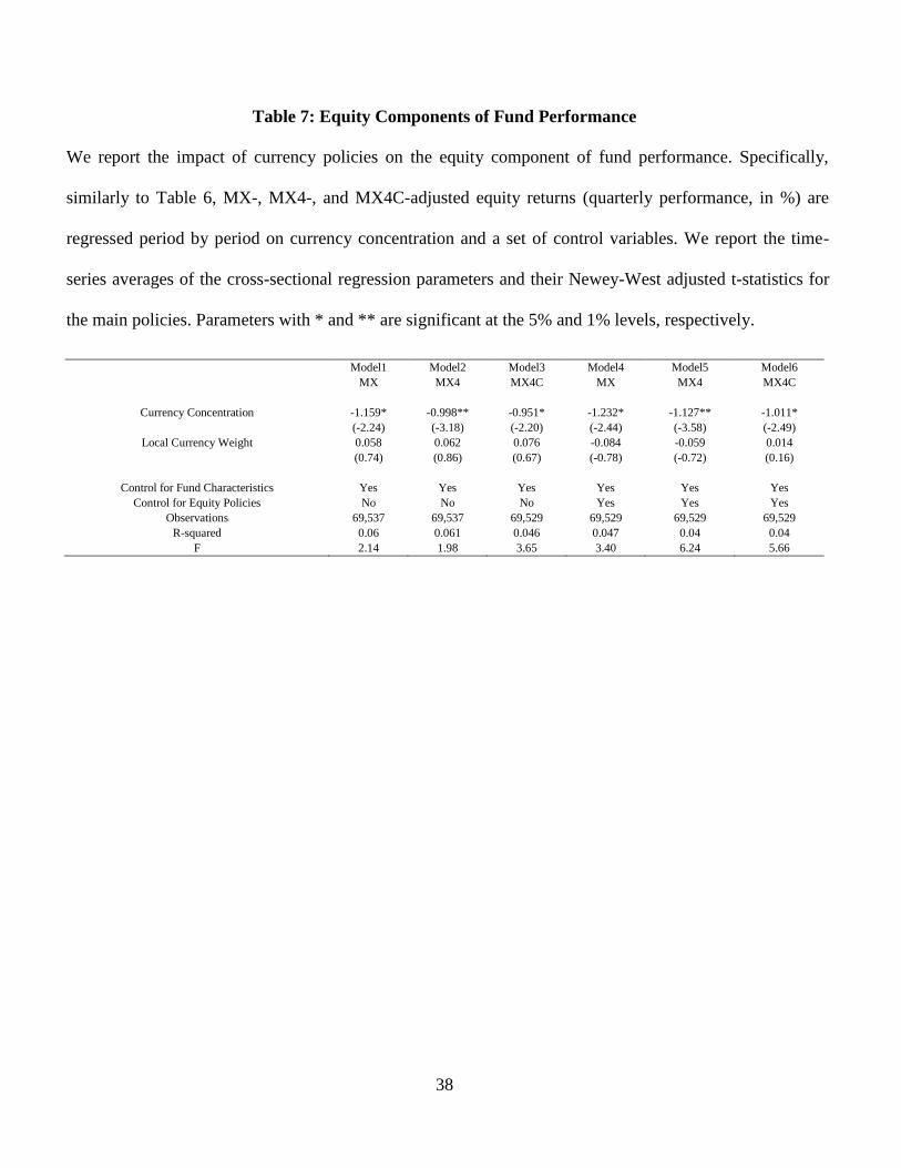
38
Table 7: Equity Components of Fund Performance
We report the impact of currency policies on the equity component of fund performance. Specifically,
similarly to Table 6, MX-, MX4-, and MX4C-adjusted equity returns (quarterly performance, in %) are
regressed period by period on currency concentration and a set of control variables. We report the time-
series averages of the cross-sectional regression parameters and their Newey-West adjusted t-statistics for
the main policies. Parameters with * and ** are significant at the 5% and 1% levels, respectively.
Model1 Model2 Model3 Model4 Model5 Model6
MX MX4 MX4C MX MX4 MX4C
Currency Concentration -1.159* -0.998** -0.951* -1.232* -1.127** -1.011*
(-2.24) (-3.18) (-2.20) (-2.44) (-3.58) (-2.49)
Local Currency Weight 0.058 0.062 0.076 -0.084 -0.059 0.014
(0.74) (0.86) (0.67) (-0.78) (-0.72) (0.16)
Control for Fund Characteristics Yes Yes Yes Yes Yes Yes
Control for Equity Policies No No No Yes Yes Yes
Observations 69,537 69,537 69,529 69,529 69,529 69,529
R-squared 0.06 0.061 0.046 0.047 0.04 0.04
F 2.14 1.98 3.65 3.40 6.24 5.66

39
Table 8: Performance Impacts of Currency Policies (Two Stages Regressions)
This table reports the out-of-sample performance impact due to various components of currency policies.
Specifically, in Panel A, we project currency concentration on ICVR and cultural distance to decompose
currency concentration into components due to ICVR, cultural distance, and other factors. Similarly to
Table 6, we then regress, in a panel specification, MX-, MX4-, and MX4C-adjusted quarterly
Morningstar total returns on various components of currency concentration and lagged control variables.
We control for the time fixed effect and estimate the error clustered at the fund level. We report the
regression parameters as well as their t-statistics for different components of currency concentration and
tabulate the parameters for other control variables in the Internet Appendix. Panels B and C report the
results for holding-implied returns and the equity component of returns, respectively. Parameters with *
and ** are significant at the 5% and 1% levels, respectively.

40
Panel A: Total Returns from Morningstar
Model1 Model2 Model3 Model4 Model5 Model6
MX MX4 MX4C MX MX4 MX4C
Fitted to ICVR -2.587** -2.178** -1.745 -2.251** -1.878** -1.511
(-4.10) (-3.76) (-1.74) (-3.66) (-3.32) (-1.51)
Fitted to Cultural Distance 0.14 -1.184** (1.12) (0.16) -1.450** (1.32)
(0.29) (-2.61) (-1.11) (-0.31) (-3.18) (-1.31)
Residual of Currency Concentration -1.043** -0.931** -0.726**
(-6.26) (-6.19) (-2.91)
Local Currency Weight -0.136 -0.086 -0.253 -0.043 -0.003 -0.189
(-1.38) (-0.94) (-1.51) (-0.45) (-0.03) (-1.13)
Control for Fund Characteristics Yes Yes Yes Yes Yes Yes
Control for Equity Policies Yes Yes Yes Yes Yes Yes
Observations 69,908 69,900 69,900 69,908 69,900 69,900
R-squared 0.009 0.011 0.012 0.011 0.013 0.013
F 9.53 13.83 5.27 10.93 15.06 5.20
Panel B: Holding Implied Returns
Model1 Model2 Model3 Model4 Model5 Model6
MX MX4 MX4C MX MX4 MX4C
Fitted to ICVR -3.185** -2.570** -2.213* -2.764** -2.195** -1.927
(-5.56) (-4.75) (-2.13) (-4.99) (-4.13) (-1.85)
Fitted to Cultural Distance 0.95 (0.52) (0.13) 0.57 (0.85) (0.39)
(1.81) (-1.08) (-0.12) (1.02) (-1.72) (-0.35)
Residual of Currency Concentration -1.305** -1.163** -0.887**
(-7.40) (-7.34) (-2.97)
Local Currency Weight -0.210* -0.213* -0.116 -0.095 -0.110 -0.037
(-2.29) (-2.45) (-0.63) (-1.09) (-1.33) (-0.20)
Control for Fund Characteristics Yes Yes Yes Yes Yes Yes
Control for Equity Policies Yes Yes Yes Yes Yes Yes
Observations 69,537 69,529 69,529 69,537 69,529 69,529
R-squared 0.008 0.008 0.008 0.01 0.01 0.009
F 8.28 9.05 3.46 11.20 11.97 3.73
Panel C: Equity Components of Fund Performance
Model1 Model2 Model3 Model4 Model5 Model6
MX MX4 MX4C MX MX4 MX4C
Fitted to ICVR -2.862** -2.145** -1.866** -2.513** -1.836** -1.612**
(-4.97) (-3.94) (-4.21) (-4.47) (-3.41) (-3.63)
Fitted to Cultural Distance 1.131* -0.242 0.219 0.819 -0.519 -0.008
(2.09) (-0.49) (0.52) (1.42) (-1.02) (-0.02)
Residual of Currency Concentration -1.084** -0.960** -0.787**
(-5.93) (-5.85) (-7.41)
Local Currency Weight -0.178* -0.139 -0.077 -0.081 -0.054 -0.007
(-1.97) (-1.63) (-1.11) (-0.94) (-0.65) (-0.10)
Control for Fund Characteristics Yes Yes Yes Yes Yes Yes
Control for Equity Policies Yes Yes Yes Yes Yes Yes
Observations 69,537 69,537 69,529 69,529 69,529 69,529
R-squared 0.007 0.009 0.008 0.009 0.008 0.009
F 7.499 9.111 7.893 9.438 31.66 33.47

41
Figure 1: Performance of Tercile Funds Sorted by Currency Concentration
In each quarter, funds are sorted into three terciles according to their lagged currency concentration. We then plot the out-of-sample
accumulated fund performance (MX-, MX4-, and MX4C-adjusted total returns) for the funds in the terciles with high and low currency
concentrations.
-10.00%
-5.00%
0.00%
5.00%
10.00%
15.00%
20.00%
Pe
rfo
rman
ce o
f Te
rcile
Fu
nd
s So
rte
d b
y C
urr
en
cy C
on
cen
trat
ion
MX,Low Currency Concentration
MX,High Currency Concentration
MX4,Low Currency Concentration
MX4,High Currency Concentration
MX4C,Low Currency Concentration
MX4C,High Currency Concentration

42
Figure 2: Impact of Currency Risk over Time
Figure 2 plots the quarterly cross-sectional regression coefficients of currency concentration based on Models 4 (MX), 5 (MX4), and 6
(MX4C) of Panel A in Table 6.
-8.0000
-6.0000
-4.0000
-2.0000
0.0000
2.0000
4.0000
6.00002
001
Ma
r
20
01 S
ep
20
02 M
ar
20
02 S
ep
20
03 M
ar
20
03 S
ep
20
04 M
ar
20
04 S
ep
20
05 M
ar
20
05 S
ep
20
06 M
ar
20
06 S
ep
20
07 M
ar
20
07 S
ep
20
08 M
ar
20
08 S
ep
20
09 M
ar
20
09 S
ep
20
10 M
ar
20
10 S
ep
20
11 M
ar
20
11 S
ep
20
12 M
ar
20
12 S
ep
Co
eff
icie
nts
of
Cro
ss S
ect
ion
al R
egr
ess
ion
s
Quarters
MX, Morningstar Total Return MX4, Morningstar Total Return MX4C, Morningstar Total Return