BENCHMARK STUDY ON MARINE COMMUNITIES OF …€¦ · Web viewESTABLISHING BENCHMARKS OF SEAGRASS...
102
ESTABLISHING BENCHMARKS OF SEAGRASS COMMUNITIES AND WATER QUALITY IN GEOGRAPHE BAY, WESTERN AUSTRALIA PROJECT CM.01B Annual report to the South West Catchments Council: September 2007 M. Westera, P. Barnes, G. Kendrick and M. Cambridge. School of Plant Biology Faculty of Natural & Agricultural Sciences The University of Western Australia 35 Stirling Highway CRAWLEY WA 6009
Transcript of BENCHMARK STUDY ON MARINE COMMUNITIES OF …€¦ · Web viewESTABLISHING BENCHMARKS OF SEAGRASS...

ESTABLISHING BENCHMARKS OF SEAGRASS COMMUNITIES AND WATER QUALITY IN GEOGRAPHE BAY, WESTERN AUSTRALIA
PROJECT CM.01B
Annual report to the South West Catchments Council: September 2007
M. Westera, P. Barnes, G. Kendrick and M. Cambridge.
School of Plant BiologyFaculty of Natural & Agricultural Sciences
The University of Western Australia35 Stirling Highway
CRAWLEY WA 6009

Establishing Benchmarks of Seagrass Communities and Water Quality in Geographe Bay 2007
Establishing benchmarks of seagrass communities and water quality in Geographe
Bay, Western Australia. Project CM.01b for the South West Catchments Council.
September 2007.
Copyright
Copyright State of Western Australia and University of Western Australia 2006. All rights reserved. This
work is copyright. Except as permitted under the Copyright Act 1968 (Cth), no part of this publication may be
reproduced by any process, electronic or otherwise, without the specific written permission of the copyright
owners. Neither may information be stored electronically in any form whatsoever without such permission.
The intellectual property rights of the data contained herein also remain with the State of Western Australia and
the University of Western Australia.
The State of Western Australia and the University of Western Australia (UWA) have made all reasonable
efforts to ensure that the contents of this document are factual and free of error. However neither the authors,
the State of Western Australia nor UWA shall be liable for any damage or loss which may occur in relation to
any person taking action or not on the basis of this document.
This report may be cited as:
Westera, M.B., Barnes, P.B, Kendrick G.A. and Cambridge M.L. (2007) Establishing benchmarks of seagrass
communities and water quality in Geographe Bay, Western Australia. Project CM.01b. September 2007.
University of Western Australia, School of Plant Biology. Report to the South West Catchments Council.
67pp.
Acknowledgements
This project was funded by the Natural Heritage Trust (NHT) which is a joint initiative of the State and
Australian Governments, and is administered by the South West Catchments Council.
We thank: Ms Joanna Hugues-Dit-Ciles, Ms Emily Hugues-Dit-Ciles and Ms Carolyn Switzer (South West
Catchments Council) and Mr Martin Heller (Australian Government Natural Resource Management Facilitator
– Coastal and Marine/Coastcare) for advice and support; Dr Malcolm Robb, Dr Helen Astill and Mr Joel Hall
(Department of Water), Ms Jenny Mitchell, Ms Kirrily White (Geocatch) for input and advice on the project
design and ongoing support; Loisette Marsh for identification of sea stars; Mr Kurt Wiegele, Mr Alexander
Grochowski, Mr Andrew Tennyson, Mr Jordan Goetze, Ms Kirrily White, Ms Heather Taylor, Mr Ben Piek, Dr
Dianne Watson, Dr Jessica Meeuwig and Dr Glenn Shiell (University of Western Australia), Mr Miles Parsons
(Curtin University) and Ms Emma Gianotti (CSIRO) for advice, support, field work and analyses; Mr Gilbert
Stokman and Mr Mike Burgess (Department of Fisheries, Busselton) for field assistance, local knowledge and
contacts; Cape Dive store in Dunsborough for staying open late to fill SCUBA cylinders; Mr Alan Miles, Mrs
Peta Miles and Mr Shane Miles at Selim Processors, Dunsborough for donating pilchards for baited remote
underwater video surveys and providing local knowledge; Professor Hans Lambers and Dr Renu Sharma
2

Establishing Benchmarks of Seagrass Communities and Water Quality in Geographe Bay 2007
(School of Plant Biology, University of Western Australia) for project management advice and financial
support; Mr Trevor Hutchison (DUIT Multimedia) for setting up the project website.
3

Establishing Benchmarks of Seagrass Communities and Water Quality in Geographe Bay 2007
Summary
The natural marine habitats of Geographe Bay face potential impacts from increases in population, growth in
tourism, recreational and commercial fishing, introduced marine pests and climate change. Decreases in
seagrass cover observed in the past coincided with extensive land clearing and drain construction during the
1950s which may have resulted in increased sediment loads and smothering of seagrasses. More recent
concerns have centred over high levels of nutrients entering Geographe Bay from agricultural and urban run-
off.
The long-term conservation of these natural habitats will require effective management, which will, in turn,
require human impacts to be identified and their effects on the ecology of the system to be understood. There
is, however, currently insufficient information to detect current impacts or predict future impacts. The
detection and understanding of human impacts is often a difficult and complex task due to the natural
background variability that exists in nature. An environmental impact study must be able to differentiate
changes caused by a human impact from natural variability. Therefore, a key step in impact assessment is to
understand the natural variability of a system. In other words, to quantify the natural patterns of spatial and
temporal distribution of marine fauna and flora – often referred to as a benchmark. Once benchmarks have
been identified, we can measure changes from place to place, or time to time. These may be changes in
biodiversity, abundances and/or sizes of particular species, or other variables that may indicate environmental
change.
Patterns of distribution of benthic habitats, seagrasses, epiphytes, fishes, invertebrates and water quality were
quantified over summer-autumn 2006-2007 in 20 sites in the seagrass meadows of southern Geographe Bay,
from Eagle Bay in the west to Forrest Beach in the east, and to 8.5 km off-shore. It should be noted that this
report does not contain results for winter sampling. Results from winter and spring sampling in Geographe Bay
are likely to be very different with higher potential nutrient loads and significantly reduced water clarity from
the catchment of Geographe Bay via drains, rivers and groundwater.
Comparisons were made based on proximity to drains and distance from shore. In general, there were no
consistent differences between sites near drains and sites distant from drains in the near-shore area. There was,
however, large spatial variability among sites in almost all the variables examined and results indicated that
environmental impacts may be occurring at smaller spatial scales localised to particular sites. For example,
high shoot density and biomass of the seagrass, Posidonia sinuosa at Toby Inlet and Siesta Park may be
indicative of localised high nutrient levels. Similarly, relatively high biomass of P. sinuosa leaves at Port
Geographe may be indicative of high nutrient levels and/or slow growth. Ongoing assessments at specific sites
in 2007 and 2008, and the inclusion of results from winter sampling, will improve our understanding of these
patterns. The detection of impacts at specific drains is likely to be valuable for the management of Geographe
Bay because it may allow targeted control of specific impacts in catchments.
Geographical trends in seagrasses and assemblages of fish were evident across Geographe Bay from Eagle Bay
to Forrest Beach. In the near-shore sites there was a relatively high cover of Amphibolis antarctica in the
central region from Buayanup Drain to Wonnerup Beach compared to relatively less cover of this species
towards the western and eastern ends of the study area. Although this pattern was correlated with the position
4

Establishing Benchmarks of Seagrass Communities and Water Quality in Geographe Bay 2007
of the drains, it is difficult to determine whether it is an impact of proximity to the drains or simply a natural
pattern of distribution across the bay. The species composition of seagrass meadows also changed with
distance from shore and increasing depth. Amphibolis antarctica and Posidonia sinuosa declined in cover
while A. griffithii increased further from shore and in deeper water. In general, the number of small rocky reefs
increased with distance from shore and depth, and is likely to have important ecological implications for fishes,
invertebrates and algae in the surrounding seagrass meadows. For example, the abundances of fish species
such as maori wrasse, western king wrasse and black headed puller were correlated with the presence of rocky
reefs or proximity to the rocky reefs associated with the Cape Naturaliste area.
Patterns of epiphyte loads on Posidonia sinuosa and artificial seagrass units (ASUs) suggested that there were
no impacts from drains occurring during the autumn period. This was expected, however, as this is usually a
time of low flows and low nutrient loading from the drains. The second time of ASU sampling will occur in
August – September 2007 to coincide with expected high nutrient loads flowing from drains during winter and
subsequent spring growth of epiphytes as water clarity improves.
Seventy six species of finfish were recorded in baited remote underwater video compared to 19 in a previous
scientific study. This difference highlights the value of using modern techniques and adequate replication to
achieve more accurate estimates of fish diversity in Geographe Bay. Species diversity of fishes was higher at
the off-shore sites followed by the near-shore, non-drain sites. Although, identifications of invertebrates are yet
to be finalised, preliminary results suggest assemblages may be relatively diverse (particularly for sponges)
compared to other temperate Australian seagrass meadows. There is also the likelihood of some sponge
species being new to science.
Preliminary estimates of nutrient levels suggest water quality could generally be considered good during the
autumn sampling period. Ammonium concentrations were, however, above the ANZECC trigger values at
several of the near-shore sites. The fact that levels were high at both drain and non-drain sites, suggests that if
high ammonium concentrations have a terrestrial origin, they are either coming via the drains and mixing well
with oceanic water, or alternatively arriving via the flow of groundwater.
The project is meeting a range of Resource Condition Targets and Management Targets as outlined by the
South West Catchments Council in the South West Regional Strategy for Natural Resource Management. The
results of sampling in winter – spring in 2007, and a repeat of summer – autumn sampling in 2008, will provide
more information regarding the potential impact of drains and rivers on the seagrass communities of Geographe
Bay. Results of summer water quality sampling should be interpreted with the understanding that winter
concentrations will be higher when drains and rivers are flowing.
5
Establishing Benchmarks of Seagrass Communities and Water Quality in Geographe Bay 2007
TABLE OF CONTENTS
1 INTRODUCTION....................................................................................................................................12
1.1 WHY DO THIS STUDY?.........................................................................................................................12
1.2 THE PROPOSED CAPES MARINE PARK AND CONSERVING BIODIVERSITY...........................................13
1.3 THE POTENTIAL FOR CHANGE IN THE MARINE ENVIRONMENT............................................................14
1.4 CONSULTATION AND PROJECT SUPPORT.............................................................................................15
Summary - Introduction............................................................................................................................................15
2 METHODS................................................................................................................................................16
2.1 PROJECT DESIGN..................................................................................................................................16
2.2 SITE SELECTION...................................................................................................................................17
2.2.1 Sites near-shore and near to drains or estuaries.......................................................................17
2.2.2 Sites near-shore and distant from drains...................................................................................17
2.2.3 Sites distant from shore (mid-shore and off-shore)....................................................................17
2.3 BENTHIC COVER..................................................................................................................................19
2.4 POSIDONIA SINUOSA.............................................................................................................................19
2.5 EPIPHYTES ON POSIDONIA SINUOSA.....................................................................................................20
2.6 EPIPHYTES ON ARTIFICIAL SEAGRASS UNITS (ASUS)........................................................................20
2.7 SAMPLING OF FISHES USING BAITED REMOTE UNDERWATER VIDEO (BRUVS)................................21
2.8 INVERTEBRATES..................................................................................................................................22
2.9 WATER QUALITY.................................................................................................................................22
2.10 DATA ANALYSES.................................................................................................................................23
2.10.1 Multivariate analyses.................................................................................................................23
2.10.2 Univariate analyses....................................................................................................................24
2.10.3 Water quality..............................................................................................................................25
Summary - Methods..................................................................................................................................................25
3 RESULTS..................................................................................................................................................26
3.1 BENTHIC COVER..................................................................................................................................26
3.1.1 Drains versus non-drains – Benthic cover.................................................................................26
3.1.2 Distance from shore – Benthic cover.........................................................................................29
Summary - Benthic cover.........................................................................................................................................31
3.2 POSIDONIA SINUOSA............................................................................................................................32
3.2.1 Drains versus non-drains – Posidonia sinuosa..........................................................................32
3.2.2 Distance from shore – Posidonia sinuosa..................................................................................33
Summary – Posidonia sinuosa..................................................................................................................................34
3.3 POSIDONIA SINUOSA EPIPHYTES..........................................................................................................35
3.3.1 Drains versus non-drains – Posidonia sinuosa epiphytes..........................................................35
3.3.2 Distance from shore – Posidonia sinuosa epiphytes..................................................................36
6

Establishing Benchmarks of Seagrass Communities and Water Quality in Geographe Bay 2007
Summary – Posidonia sinuosa epiphytes.................................................................................................................37
3.4 ARTIFICIAL SEAGRASS UNITS (ASUS).................................................................................................38
3.4.1 Drains versus non-drains - ASUs...............................................................................................38
3.4.2 Distance from shore - ASUs.......................................................................................................39
Summary – Artificial seagrass units.........................................................................................................................40
3.5 BAITED REMOTE UNDERWATER VIDEO (BRUVS)..............................................................................41
3.5.1 Drains versus non-drains - BRUVs............................................................................................41
3.5.2 Distance from shore - BRUVs....................................................................................................44
Summary - Baited remote underwater video of fishes..............................................................................................49
3.6 NON-CRYPTIC MOBILE AND SESSILE BENTHIC INVERTEBRATES..........................................................50
3.6.1 Corals and zoanthids..................................................................................................................50
3.6.2 Echinoderms (sea stars, sea urchins and sea cucumbers).........................................................51
3.6.3 Ascidians (Sea squirts)...............................................................................................................52
3.6.4 Sponges.......................................................................................................................................53
3.6.5 Molluscs......................................................................................................................................54
Summary - invertebrates...........................................................................................................................................54
3.7 WATER QUALITY – MARCH 2007.......................................................................................................54
Summary – Water quality – March 2007..................................................................................................................57
4 DISCUSSION............................................................................................................................................58
4.1.1 Benthic cover..............................................................................................................................59
4.1.2 Posidonia sinuosa.......................................................................................................................60
4.1.3 Epiphytes on Posidonia sinuosa.................................................................................................60
4.1.4 Artificial Seagrass Units (ASUs)................................................................................................60
4.1.5 Baited Remote Underwater Video (BRUVs)...............................................................................60
4.1.6 Non-cryptic sessile and mobile invertebrates.............................................................................61
4.1.7 Water quality..............................................................................................................................61
4.2 PROJECT OUTCOMES............................................................................................................................62
Summary - Discussion..............................................................................................................................................63
5 REFERENCES.........................................................................................................................................64
6 APPENDIX - DATA TABLE..................................................................................................................66
TABLE OF FIGURES
Figure 2.2.1: Sites sampled in Geographe Bay. ○ - Sites near-shore and near to drains, ○ – Sites near-shore and distant
from drains, ○ - Mid-shore sites, ○ - Off-shore sites. Source: Google Earth 2007......................................................18
Figure 2.6.1: Artificial seagrass units (ASUs) deployed in a Posidonia sinuosa meadow in Geographe Bay.....................21
Figure 2.7.1: Baited Remote Underwater Video (BRUV) unit. Note: two forward facing video cameras secured to frame.
.......................................................................................................................................................................................22
7

Establishing Benchmarks of Seagrass Communities and Water Quality in Geographe Bay 2007
Figure 3.1.1: MDS ordination illustrating differences in the composition of benthic cover at each site. Sites away from
drains are presented in green and sites near to drains are in red...................................................................................27
Figure 3.1.2: Percentage cover of the most common vegetation (mean + S.E.) and number of rocky reefs (mean + S.E.) per
benthic transect at each near-shore site. Sites away from drains are highlighted in green and sites near drains are in
red. The sites are presented in geographical order from west (Eagle Bay) to east (Forrest Beach)............................28
Figure 3.1.3: MDS ordination illustrating differences in assemblages in replicate benthic transects at each site. Near-
shore sites are presented in green, mid-shore sites in light blue and off-shore sites in dark blue.................................29
Figure 3.1.4: Percentage cover of the most common vegetation (mean + S.E.) and number of rocky reefs (mean + S.E.)
per benthic transect at each site. Near-shore sites are presented in green, mid-shore sites in light blue and off-shore
sites in dark blue............................................................................................................................................................30
Figure 3.2.1: Number of shoots m-2, shoot height (cm), biomass (g.m-2 of seafloor), and leaf area index (LAI) measured in
m2 of Posidonia sinuosa leaves per m2 of seafloor (mean + S.E.). For ease of comparison with other studies, data
have been converted from numbers per quadrat (0.04 m2) to numbers per m2. Sites away from drains are highlighted
in green and sites near drains are in red. The sites are presented in geographical order from west (Eagle Bay) to east
(Forrest Beach)..............................................................................................................................................................32
Figure 3.2.2: Number of shoots m-2, shoot height (cm), biomass (g.m-2 of seafloor), and leaf area index (LAI) measured in
m2 of Posidonia australis leaves per m2 of seafloor (mean + S.E.). For ease of comparison with other studies, data
have been converted from numbers per quadrat (0.04 m2) to numbers per m2. Near-shore sites are presented in
green, mid-shore sites in light blue and off-shore sites in dark blue.............................................................................33
Figure 3.3.1. Dry weight (g) of epiphytes per m2 of Posidonia sinuosa leaf, % ash free dry weight and % CaCO3 (mean
+SE). Non-drain sites are presented in green and drains are in red. The sites are presented in geographical order
from west (Eagle Bay) to east (Forrest Beach).............................................................................................................35
Figure 3.3.2: Dry weight (g) of epiphytes per m2 of Posidonia sinuosa leaf, % ash free dry weight and % CaCO3 (mean
+SE). Near-shore sites are presented in green, mid-shore sites in light blue and off-shore sites in dark blue............36
Figure 3.4.1: ASU showing epiphyte growth after 8 weeks in Geographe Bay...................................................................38
Figure 3.4.2: Dry weight (mg) of epiphytes per cm2 of ASU, % ash free dry weight and % CaCO3. (mean +S.E.) Non-
drains are presented in green and drains in red. The sites are presented in geographical order from west
(Dunsborough) to east (Forrest Beach).........................................................................................................................38
Figure 3.4.3: Dry weight (g) of epiphytes per m2 of ASU, % ash free dry weight and % CaCO3 (mean + S.E.). Near-shore
sites are presented in green, mid-shore sites in light blue and off-shore sites in dark blue..........................................39
Figure 3.5.1: MDS ordination illustrating differences in assemblages of fish in replicate Baited Remote Underwater
Videos at each site. Sites away from drains are presented in green and sites near to drains are in red. Note: caution
should be used in interpreting this MDS because the relatively high stress value of 0.21 suggests the ordination may
be not adequately represent real patterns of difference among samples.......................................................................41
Figure 3.5.2: Maximum numbers of trumpeter (Pelates sexlineatus), sand trevally (Pseudocaranx wrightii), yellowtail
scad (Trachurus novaezelandiae), gobbleguts (Apogon ruepellii), silver belly (Parequula melbournensis) and silver
trevally (P. dentex) observed with Baited Remote Underwater Videos (BRUVS) in near-shore sites. Non-drain sites
are highlighted in green and drain sites are in red. The sites are presented in geographical order from west (Eagle
Bay) to east (Forrest Beach)..........................................................................................................................................43
Figure 3.5.3: MDS ordination illustrating differences in assemblages in assemblages of fish in replicate Baited Remote
Underwater Videos. Near-shore sites are presented in green, mid-shore sites in light blue and off-shore sites in dark
blue................................................................................................................................................................................45
Figure 3.5.4: Maximum numbers of striped trumpeter (Pelates sexlineatus), silver belly (Parequula melbournensis),
yellowtail scad (Trachurus novaezelandiae), silver trevally (Pseudocaranx. dentex), orange spotted wrasse
(Notolabrus parilus), western king wrasse (Coris auricularis), maori wrasse (Ophthalmolepis lineolatus) and black
headed puller (Chromis klunzingeri) counted in BRUVs. Near-shore sites are presented in green, mid-shore sites in
light blue and off-shore sites in dark blue.....................................................................................................................47
8

Establishing Benchmarks of Seagrass Communities and Water Quality in Geographe Bay 2007
Figure 3.5.5: Examples of fishes observed in Baited Remote Underwater Videos...............................................................48
Figure 3.6.1: Examples of corals found in Geographic Bay.................................................................................................50
Figure 3.6.2: Examples of echinoderms found in Geographe Bay........................................................................................51
Figure 3.6.3: Examples of ascidians found in Geographe Bay.............................................................................................52
Figure 3.6.4: Examples of sponges found in Geographe Bay. Species are to be identified by the Western Australian
Museum.........................................................................................................................................................................53
Figure 3.7.1: Comparisons of nutrient and chlorophyll a concentrations sampled in the current study (red or green bars)
with data collected in comparable sites in 1994 by McMahon and Walker (1997) (open bars) and in 2002 by Sinclair
Knight and Merz (2003) (grey bars). Dashed lines represent ‘trigger’ values set by the Australian and New Zealand
Environmental Conservation Council and solid lines represent concentrations recorded in Warnbro Sound (DEP
(WA), 1996). * indicates concentrations were below limits of detection....................................................................55
TABLE OF TABLES Table 2.2.1: The location, site code, proximity to drains, distance from shore and depth for study sites in Geographe Bay.
.......................................................................................................................................................................................18
Table 2.3.1: Categories of benthic organisms and inorganic substrata identified in video transects.....................................19
Table 3.1.1: Summary of R values from ANOSIM pairwise comparisons of the composition of benthic cover between
pairs of sites in near-shore habitats. Sites significantly different at p < 5% are in bold. See Table 2.2.1 for
abbreviations of site names. Note: R values < 0.3 although significant, indicate a relatively small difference in
composition...................................................................................................................................................................27
Table 3.1.2: Results of analyses of variance to test for differences in selected variables between sites near to drains
compared to sites away from drains. ns – not significant, * - p < 0.05, *** - p < 0.001. MS = mean square, F = F
ratio and p = probability in this and all subsequent ANOVA tables.............................................................................29
Table 3.1.3: Results of analyses of variance to test for differences in % cover of selected variables and numbers of rocky
reefs with distance from shore. ns – not significant, * - p < 0.05, *** - p < 0.001....................................................31
Table 3.2.1: Results of analyses of variance to test for differences in shoot density, shoot height, total biomass and leaf
area index near to drains compared to away from drains. ns – not significant, *** - p < 0.001. a heterogeneity of
variances was not removed after transformation...........................................................................................................33
Table 3.2.2: Results of analyses of variance to test for differences in shoot density, shoot height, total biomass and leaf
area index with distance from shore. ns – not significant, *** - p < 0.001................................................................34
Table 3.3.1: Results of analyses of variance to test for differences in dry weight, % ash free dry weight (AFDW) and %
CaCO3 near to drains compared to away from drains. ns – not significant, *** - p < 0.001. a heterogeneity of
variances was not removed after transformation...........................................................................................................36
Table 3.3.2: Results of analyses of variance to test for differences in dry weight, % Ash Free Dry Weight (AFDW) and %
CaCO3 with distance from shore. ns – not significant, * - p < 0.05, * - p < 0.01, *** - p < 0.001. a heterogeneity of
variances was not removed after transformation...........................................................................................................37
Table 3.4.1: Results of PERMANOVA analyses to test for differences in dry weight, % ash free dry weight (AFDW) and
% CaCO3 on ASUs near drains compared to away from drains. ns – not significant, *** - p < 0.001.....................39
Table 3.4.2: Results of PERMANOVA analyses to test for differences in dry weight, % ash free dry weight (AFDW) and
% CaCO3 on ASUs with distance from shore. ns – not significant, *** - p < 0.001.................................................40
Table 3.5.1: Measures of diversity of fishes recorded in each type of habitat. Sites were pooled in each habitat type.......41
Table 3.5.2: Summary of R values from ANOSIM comparing assemblages of fishes between pairs of sites in near-shore
habitats. Bold type indicates pairs of sites that are significantly different at p < 5%. See Table 2.2.1 for explanation
of abbreviations of site names.......................................................................................................................................42
Table 3.5.3: Results of analyses of variance to test for differences in Maximum Number of striped trumpeter, sand
trevally, yellowtail scad, western gobbleguts, silver belly and silver trevally in sites near drains compared to sites
9
Establishing Benchmarks of Seagrass Communities and Water Quality in Geographe Bay 2007
away from drains. ns – not significant, * - p < 0.01, ** - p < 0.01, *** - p < 0.001. a heterogeneity of variances was
not removed after transformation..................................................................................................................................44
Table 3.5.4: Results of analyses of variance to test for differences with distance from shore in Maximum Numbers of
striped trumpeter, silver belly, sand trevally, yellowtail scad, silver trevally, Notolabrus parilus, western king wrasse,
Maori wrasse and black headed puller counted in BRUVs. ns – not significant, * - p < 0.05, ** - p < 0.01, *** - p <
0.001. a heterogeneity of variances was not removed after transformation..................................................................46
Table 3.7.1: Measurements of water quality recorded in Geographe Bay in March 2007....................................................56
Table 4.2.1: Summary of Resource Condition Targets (RCTs) and Management Targets (MTs) for NHT and NAP projects
and how these have been addressed by Project CM.01b. See Section 1.1 for full details of RCTs and MTs.............63
Table 4.2.1: Mean abundance (Max N) of fish species recorded in baited remote underwater video (BRUV) at each site
(see Table 2.2.1 for site codes). Some identifications are to be finalised and are marked unknown or presented as the
genus followed by sp.....................................................................................................................................................66
10
Establishing Benchmarks of Seagrass Communities and Water Quality in Geographe Bay 2007
1 INTRODUCTION
This report presents the findings of the first year of the South West Catchments Council Project CM.01b
“Establishing benchmarks of seagrass and water quality in Geographe Bay, Western Australia”. The
objectives of the project, as outlined by the South West Catchments Council, were to establish comprehensive
baselines of information on seagrasses, epiphytes, fishes, invertebrates and water quality from representative
sites within Geographe Bay. The data will be used to develop resource condition targets for long term
monitoring and management of the marine environment of Geographe Bay.
1.1 WHY DO THIS STUDY?
The natural marine habitats of Geographe Bay face potential impacts from increases in population, growth in
tourism, recreational and commercial fishing, introduced marine pests and climate change. Decreases in
seagrass cover observed in the past coincided with extensive land clearing and drain construction during the
1950s which may have resulted in increased sediment loads and smothering of seagrasses (Lord and
Associates, 1995). More recently concerns have centred over high levels of nutrients entering Geographe Bay
from agricultural and urban run-off (Lord and Associates, 1995; McMahon et al., 1997; SKM, 2003).
The long-term conservation of these natural habitats will require effective management, which will, in turn,
require human impacts to be identified and their effects on the ecology of the system to be understood. There
is, however, currently insufficient information to detect current impacts or predict future impacts. The
detection and understanding of human impacts is often a difficult and complex task due to the natural
background variability that exists in nature. An environmental impact study must be able to differentiate
changes caused by a human impact from natural variability. Therefore, a key step in impact assessment is to
understand the natural variability of a system. In other words, to quantify the natural patterns of spatial and
temporal distribution of marine fauna and flora – often referred to as a benchmark. Once benchmarks have
been identified, we can measure changes from place to place, or time to time. These may be changes in
biodiversity, abundances and/or sizes of particular species, or other variables that may indicate environmental
change.
The South West Catchments Council (SWCC), as part of their Regional Strategy for Natural Resource
Management (SWCC, 2005) recognised the need to gain a better understanding of the marine environments
and ecology of Geographe Bay and consequently commissioned the University of Western Australia to do a
benchmark study of the marine flora and fauna associated with seagrass communities in Geographe Bay. The
long-term conservation of Geographe Bay requires: an understanding of the natural patterns of distribution of
marine fauna and flora and the biodiversity of the region (i.e. identifying benchmarks), identification of
environmental impacts, and an understanding of the effects of any impacts on the ecology and functioning of
these systems. This project represents the logical and essential first step in this process. In addition, this
project makes a preliminary investigation of potential point sources of environmental impact – i.e. drains and
estuaries which may discharge nutrient enriched and/or turbid water into the bay. It must be noted, however,
that this study does not and was not designed to test for small scale impacts of individual drains. Rather, it
provides a comprehensive assessment of broadscale patterns in seagrass communities from representative
11
Establishing Benchmarks of Seagrass Communities and Water Quality in Geographe Bay 2007
sites throughout Geographe Bay and the necessary information to design more intensive and targeted
assessments for specific areas which show signs of potential environmental degradation.
Included in the SWCC Regional Strategy were Marine Resource Condition Targets (RCTs), Marine Targets
(MTs) and Management Actions (SWCC, 2005). The data collected in Project CM.01b will contribute
significantly toward achieving RCTs and MTs for Geographe Bay and the SW region. Those targets relevant
to Project CM.01b have been listed below. More information on how these have been addressed is provided
in section 4.2 Project outcomes. Relevant targets from the South West Regional Strategy for Natural
Resource Management (SWCC, 2005) include:
MRCT1: Marine habitat integrity to be improved by 2025.
MT1: Gaps in marine knowledge to be identified. Management Actions - MT1.2: Determine condition
and status of key habitats and ensure protection of these habitats.
MT4: Critical marine ecosystem processes for the ongoing conservation of the most threatened
biodiversity assets are identified and documented. Management Actions - MT4.2: Research marine
ecosystem processes identified as critical to long-term conservation needs.
MT5: Baseline information on the ecological condition of key marine species and ecosystems is
documented.
MT9: A long term monitoring program of at-risk ecosystems, communities, habitats and species is
developed and implemented. Management Actions - MT9.1: Develop monitoring of selected key
biodiversity assets (species, communities and ecosystems).
MT10: The conservation status of at-risk and special species, communities and ecosystems are
evaluated by 2009. Management Actions - MT10.1: Develop monitoring of selected key biodiversity
assets (species, communities and ecosystems); MT10.2: Monitor population trends of selected at-risk
species; and MT10.4: Identify regionally significant species, communities and ecosystems in the SW
region.
MT21: Community awareness of the SW regions marine biodiversity, habitat integrity and threats to
be increased.
WRCT 16: Reduce water related point source and diffuse pollution in the region by 2024. WT1:
Standard water quality data set and resource health inventory for waterways, wetlands and estuaries by
2008.
1.2 THE PROPOSED CAPES MARINE PARK AND CONSERVING BIODIVERSITY
In 2005 and 2006 the Government of Western Australia and the Marine Parks and Reserves Authority
commenced a consultation process with the people of Western Australia to establish a marine park in the
Capes region. This includes a network of sanctuary zones, three of which are proposed for Geographe Bay.
The Indicative Management Plan for the Marine Park can be downloaded from the Department of
Environment and Conservation website http://www.naturebase.net/ and contains charts with the proposed
zoning of the Marine Park.
12

Establishing Benchmarks of Seagrass Communities and Water Quality in Geographe Bay 2007
The original objectives of this project (see ) did not include assessment of proposed sanctuary zones in
Geographe Bay. However, we were able to locate two sites in the present study (MS2 and MS4) to be
contained within the boundaries of the proposed reserves. The location of these sites will provide some
information on the effectiveness of the reserves by comparing changes in marine fauna and flora from before
to after protection. However, to further build knowledge on the effect of sanctuary zones on seagrass
communities, permanent monitoring sites will be established within proposed sanctuary zones in 2007-08, in
association with the Department of Conservation and Environment - Marine Impacts Branch.
1.3 THE POTENTIAL FOR CHANGE IN THE MARINE ENVIRONMENT
The population of the southwest region is estimated to increase from its current size of approximately 135,000
to 220,000 by the year 2030. Tourism is also estimated to increase from 3.5 million tourist nights in 2002 to
7.5 million in 2030 (Southwest Development Commission, 2004). Increases in population and tourism will
require effective management to minimise any impacts to the marine environment. The major threat to the
marine environment of Geographe Bay associated with this growth will be changes to water quality due to
inputs of nutrients (i.e. nitrogen and phosphorus) which may come from residential and agricultural areas,
septic sewage systems or treated sewage outfalls. Seagrasses communities are particularly susceptible to
changes in water quality. For example, extensive losses of seagrasses from Cockburn Sound (77%) since the
1960s have been largely attributed to nutrient enrichment from terrestrial run-off, which can cause excessive
growth of epiphytic algae and subsequent shading of seagrass leaves (Cambridge et al., 1986; Kendrick et al.,
2002).
Other impacts to the marine environment of Geographe Bay may arise from introduced marine pests, fishing
pressure, oil spills, coastal developments (marinas and canal estates) and severe weather events. Introduced
marine pests are becoming increasingly recognised as problematic across Australia. Introductions have been
recorded in Cockburn Sound (fan worm), Darwin (striped mussel) and Tasmania (North Pacific sea star and
the alga Undaria). In New South Wales there is also concern that the introduced green alga, Caulerpa
taxifolia is replacing endemic seagrasses. The first step in managing introduced species is detecting their
presence. Many introduced species, however, go relatively unnoticed until they begin to cause environmental
impacts. The broad-scale nature of the current study provides an important mechanism for detection of
introduced species in Geographe Bay.
Climate change may lead to changes in seawater temperatures, rising sea levels and changes in water
chemistry which may also cause long-term changes in the marine communities of Geographe Bay. The
identification of benchmarks through an understanding of natural patterns of distribution of marine fauna and
flora is an essential first step in detecting impacts of these processes on the marine environment.
13
Establishing Benchmarks of Seagrass Communities and Water Quality in Geographe Bay 2007
1.4 CONSULTATION AND PROJECT SUPPORT
An important component of this project was to consult with key organisations that may have an interest in the
management of the marine environment of Geographe Bay. Details of the project were discussed and input
sought in the initial stages of the project. The project design builds on the ‘Recommendations for future
monitoring of the seagrass ecosystem in Geographe Bay’ (White et al., 2006) and was developed in
consultation with scientists and managers from the University of Western Australia, the South West
Catchments Council, Geocatch, and the Department of Water (DoW) (then the Department of Environment).
Further collaboration is underway with the Department of Environment and Conservation (DEC).
Ongoing consultation, advice and support have been facilitated by presenting the project findings and
engaging the media. The project findings have been presented to the: University of Western Australia, School
of Plant Biology – November 2006; South West Catchments Council (SWCC) - January 2007; Western
Australian Marine Science Institute (WAMSI) – March 2007; Geocatch – May 2007; South West and Peel
Coastal Management Group (CoastSWap) - June 2007; Department of Environment and Conservation (DEC)
– August 2007; and Department of Water (DoW) - September 2007. Further meetings have been held with
professional fishers in the region and with the Busselton Underwater Observatory.
The project has direct links with the Australian and West Australian Government “Coastal Catchments
Initiative”, the University of Western Australia Marine Futures project “Setting Marine Resource Condition
Targets for Temperate Western Australia”, and projects from the Department of Water “South West Decision
Support Modelling DOW SWCC W3-02” and “Near-shore Contaminants C1-01”.
SUMMARY - INTRODUCTION
High population growth is forecast for the Capes region
Current concern over impacts from nutrient rich agricultural and urban run-off and groundwater
Increases in population and tourism may impact the marine environment by increasing pressure on
resources
Other impacts may arise from climate change and/or introduced marine species
Currently insufficient information to detect current or predict future impacts
Project will provide benchmarks and resource condition targets by quantifying natural patterns of
distribution and abundance of marine flora and fauna
Current project design incorporates sites within proposed sanctuary zones of the Capes Marine Park
14

Establishing Benchmarks of Seagrass Communities and Water Quality in Geographe Bay 2007
2 METHODS
2.1 PROJECT DESIGN
The design for this project builds on the ‘Recommendations for future monitoring of the seagrass ecosystem
in Geographe Bay’ (White et al., 2006) which was commissioned by SWCC in 2005. The sampling was
focussed on Posidonia sinuosa which is the dominant meadow forming seagrass in Geographe Bay. The
study area encompasses the seagrass meadows of southern Geographe Bay from Eagle Bay to Forrest Beach
and to approximately 8.5 km off-shore (Figure 2.2.1). Sampling was designed to test for differences in water
quality, seagrass characteristics and fauna: near to, and distant from, known point sources of nutrients (i.e.
drains and natural estuary openings); and with increasing depth and distance from shore. The inclusion of
sites with increasing depth and distance from shore provides the necessary broad baseline data to detect
temporal changes over large spatial scales in Geographe Bay. This is important because, although short term
impacts or changes are likely to be most evident in near shore habitats, off-shore and deeper habitats may also
be affected, particularly with climate change. Additionally, elevated nutrients in the water column which may
affect seagrasses are likely to decrease with increasing distance from shore, due to uptake by marine
organisms and dilution by mixing with oceanic waters. The inclusion of off-shore sites thus provides a
comparison of seagrass communities along a potential gradient of nutrient concentrations.
In addition to making spatial comparisons among sites, depths and proximity to drains, an important
component of this project is to examine temporal changes in communities. Natural communities tend to vary
through time in terms of the abundance and biomass of organisms. Thus, studies which include multiple
times of sampling provide more comprehensive baselines by including natural variation through time. An
understanding of natural variation then allows more confident assessments to be made of longer-term changes
and assessments of environmental impacts. Furthermore, environmental impacts may have short or long-term
effects (Glasby et al., 1996). This concept is particularly relevant for Geographe Bay, where historically there
have been pulses of potentially nutrient enriched freshwater entering the bay from drains during the winter
months (SKM, 2003). These pulses may have long-term impacts on the marine environment of Geographe
Bay, short term impacts that are only evident at certain times of the year, or no impact at all. Short-term
effects from an impact are likely to be seen in relatively fast growing organisms (e.g. epiphytic algae) and/or
mobile organisms (e.g. fishes) which can recover or recolonise relatively quickly. In this study, major
sampling of a range of organisms (seagrasses, fishes, invertebrates and epiphytes) was done over the
summer/autumn period when relatively high water clarity made sampling practical. Sampling during this
period allowed potential long-term effects of impacts to be identified. Additional sampling will be done
during winter/spring 2007 with the aim of detecting shorter-term effects on epiphyte growth and water
quality. Summer/autumn sampling will also be repeated in 2007-08.
15
Establishing Benchmarks of Seagrass Communities and Water Quality in Geographe Bay 2007
2.2 SITE SELECTION
Four types of sampling sites were chosen in Geographe Bay (described below) based on distance from
shore/depth and proximity to drains or estuaries:
1. Near-shore and near to drains or estuaries
2. Near-shore and away from drains
3. Mid-shore
4. Off-shore
Five sites were chosen in each category using a combination of aerial photography, nautical charts and habitat
maps. The suitability of prospective sites was confirmed in the field using a video camera lowered to the
seafloor while an observer viewed the underwater image on a screen on the boat.
2.2.1 SITES NEAR-SHORE AND NEAR TO DRAINS OR ESTUARIES
There are a number of drains and natural estuary openings which flow into Geographe Bay. Each has the
potential to cause existing and/or future impacts in the Bay. A subset of five was chosen and included in this
study. Sites were approximately 350 – 600 m off-shore from the drains or estuary openings, within seagrass
meadows and in 3-5 m depth of water. For conciseness of text, these sites are referred to as ‘drains’ in the
remainder of the report.
2.2.2 SITES NEAR-SHORE AND DISTANT FROM DRAINS
The location of sites away from drains and near-shore was partly limited by the relatively large number of
drains and estuary openings in the central region of Geographe Bay from Buayanup Drain to the Vasse
Wonnerup estuary. In an ideal scenario, sites away from drains would be interspersed with sites near drains
throughout the study region. However, with the exception of Siesta Park, there were few long stretches of
shoreline without drains. Therefore, two sites were chosen away from drains in the south west of the study
region and two sites towards the north eastern end of the study region, in areas without large drains or
estuaries. Sites were at least 1.5 km from any drain or estuary opening. For conciseness of text, these sites
are referred to as ‘non-drains’ in the remainder of the report.
2.2.3 SITES DISTANT FROM SHORE (MID-SHORE AND OFF-SHORE)
In addition to the near-shore sites, five sites were sampled in each of what were categorised as the mid-shore
and off-shore regions of Geographe Bay. Mid-shore sites were located in approximately 8-12 m depth and
were approximately 2.5 - 4.5 km from shore depending on the slope of the seafloor. Off-shore sites were
located in approximately 15-18 m depth and were approximately 4.5 – 8.5 km from shore depending on the
slope of the seafloor. Note that distance from shore and depth are strongly correlated and in terms of their
potential ecological effects should not be interpreted separately. However, for conciseness of text only,
reference to depth is omitted from site descriptions in the remainder of the methods and results.
16
Establishing Benchmarks of Seagrass Communities and Water Quality in Geographe Bay 2007
Table 2.2.1: The location, site code, proximity to drains, distance from shore and depth for study sites in Geographe Bay.
Location Site code Proximity to drains
Distance from Shore
Depth
Toby Inlet TI Near Near 3-5 mBuayanup Drain BD Near Near 3-5 mVasse Diversion Drain VD Near Near 3-5 mPort Geographe PG Near Near 3-5 mVasse Wonnerup VW Near Near 3-5 mEagle Bay EB Far Near 3-5 mDunsborough DU Far Near 3-5 mSiesta Park SP Far Near 3-5 mWonnerup Beach WB Far Near 3-5 mForrest Beach FB Far Near 3-5 mMid-shore Site 1 MS1 Far Mid 8-12 mMid-shore Site 2 MS2 Far Mid 8-12 mMid-shore Site 3 MS3 Far Mid 8-12 mMid-shore Site 4 MS4 Far Mid 8-12 mMid-shore Site 5 MS5 Far Mid 8-12 mOff-shore Site 1 OS1 Far Off 15-20 mOff-shore Site 2 OS2 Far Off 15-20 mOff-shore Site 3 OS3 Far Off 15-20 mOff-shore Site 4 OS4 Far Off 15-20 mOff-shore Site 5 OS5 Far Off 15-20 m
Figure 2.2.1: Sites sampled in Geographe Bay. ○ - Sites near-shore and near to drains, ○ – Sites near-shore and
distant from drains, ○ - Mid-shore sites, ○ - Off-shore sites. Source: Google Earth 2007
17
Establishing Benchmarks of Seagrass Communities and Water Quality in Geographe Bay 2007
2.3 BENTHIC COVER
Benthic cover was measured to assess habitat differences among sites. In each site, benthic cover data was
collected along six haphazardly chosen 25 m transects using a hand-held video camera positioned
approximately 50 cm above the seafloor. In the laboratory, video footage from each transect was processed to
determine the percentage cover of 22 categories of organisms and inorganic substrata (Table 2.3.2).
Categories were chosen based on the level of identification possible from the video footage. In general, the
seagrasses and some of the more distinctive species of macroalgae could be identified to species or genus.
Smaller and less distinctive species of algae that could not be reliably identified from the footage were
grouped in the category – unidentifiable algae. Similarly, most invertebrates including sponges, corals,
ascidians and sea stars could not be identified to species from the video footage and were classified into their
respective groups. The percentage cover of each benthic type in each transect was estimated by determining
the category of cover under each of 10 points in each of 15 randomly selected frames (a total of 150 points per
transect).
A second method of video analysis was used to estimate the numbers of patches of rocky reef. Preliminary
analysis of the video footage suggested small patches of rocky reef were relatively sparse and therefore
unlikely to be found in individual frames. The presence of even small patches of rocky reef, however, has the
potential to influence assemblages of fish, invertebrates and vegetation and it is, therefore, important to
estimate their extent. Therefore, the total number of patches of rocky reef were counted along the entire
length of each transect.
Table 2.3.2: Categories of benthic organisms and inorganic substrata identified in video transects.
Seagrasses Algae Invertebrates Inorganic
Amphibolis antarctica Caulerpa spp. Ascidians Bare reef
Amphibolis griffithii Cystophora racemosa. Corals Rubble
Halophila spp. Padina australis Sponges Shell grit
Posidonia australis Sargassum spp. Sea stars Sand
Posidonia sinuosa Udotea spp. Other invertebrates
Dead rhizomes or stems Unidentifiable algae
Seagrass wrack
2.4 POSIDONIA SINUOSA
Posidonia sinuosa (seagrasses) were collected by SCUBA divers in six replicate 20 × 20 cm quadrats at each
site. Quadrats were placed haphazardly within patches of P. sinuosa. Samples were frozen and returned to
the laboratory where the number of shoots was counted, and average leaf height, biomass and leaf area were
measured for each sample. An average leaf height was estimated for each sample using the standard methods
described by Duarte and Kirkman (2001). In this method, leaves are extended to their maximum height and a
measurement is made from the base of the leaves to the top of 80 % of the leaves, ignoring the tallest 20 %.
Biomass was measured as grams of dry weight after drying in an oven at 105°C until constant weight was
reached. Biomass was determined after epiphytes had been scraped from each leaf (see section 2.5). Leaf
18

Establishing Benchmarks of Seagrass Communities and Water Quality in Geographe Bay 2007
area was estimated for each sample by photographing a subset of leaves against a background of known grid
size and analysing the images with the computer programme, Sigmascan. The subset of leaves was weighed
separately from the remaining sample. The total leaf area for each sample was then calculated as:
A multiplier of 2 was used to account for both sides of the leaves. Data were converted to cm2 of leaf area per
m2 of substrata to aid in comparisons with other studies.
2.5 EPIPHYTES ON POSIDONIA SINUOSA
In the laboratory, epiphytes were removed from the Posidonia sinuosa leaves using a razor blade and dried at
90°C for dry weight, 550°C for Ash-Free-Dry-Weight (AFDW) and 950°C to determine calcium carbonate
content (CaCO3). High AFDW may be indicative of high loads of epiphyte species which respond to nutrient
enrichment, whereas high proportions of CaCO3 generally indicate lower nutrient concentrations in the water
column (Cambridge et al., 1986).
2.6 EPIPHYTES ON ARTIFICIAL SEAGRASS UNITS (ASUS)
In addition to Posidonia sinuosa leaves, epiphyte biomass was also measured on Artificial Seagrass Units
(ASUs). Technically, epiphytes which grow on non-living substrata are termed ‘periphyton’, however, for
clarity and consistency we use the term epiphyte throughout the text. While sampling epiphytes on natural
seagrass leaves is useful in identifying environmental perturbations such as increases in water column
nutrients, comparisons among sites can be potentially confounded by the natural variability of the
morphology, density, age, etc. of seagrass leaves. The use of artificial leaves overcomes this problem by
providing a standard size and age of substratum on which the epiphytes can grow. Furthermore, epiphytes
readily colonise artificial substrata, with similar settlement and growth patterns to natural seagrasses (Harlin,
1973; Silberstein et al., 1986; Horner, 1987; Neverauskus, 1987). These qualities and the uniform
morphology of artificial seagrass leaves allow unconfounded comparisons of epiphyte growth to be made
among sites.
In this study, ASUs were constructed to resemble Posidonia sinuosa shoots (Figure 2.6.2). Each ASU
consisted of 16 ‘shoots’ made from 60 × 1 cm strips of 200 μm clear polyethylene. Each strip was folded
around a plastic base grid and stapled to form two leaves: one 40 cm and one 20 cm. Grids were
approximately 13 cm × 15 cm with rectangular apertures of approximately 1.2 cm × 1.5 cm. Six replicate
ASUs were secured to the seafloor in each site (with the exception of Eagle Bay) with galvanised steel pegs.
ASUs were collected 8 weeks after deployment, frozen and returned to the laboratory. A deployment of eight
weeks was necessary during the summer period for sufficient biomass to accumulate for laboratory analyses.
Eight weeks was also considered an appropriate duration of deployment during the upcoming winter/spring
period to allow epiphyte growth when nutrients are expected to flow from drains into the bay, and then
subsequent increases in water clarity in spring which would allow sufficient light for epiphyte growth.
19

Establishing Benchmarks of Seagrass Communities and Water Quality in Geographe Bay 2007
Epiphytes on ASUs were removed and dried using the same methods as were used for the natural P. sinuosa
leaves. Epiphytes were removed using a razor blade and dried at 90°C for dry weight, 550°C for Ash-Free-
Dry-Weight (AFDW) and 950°C to determine calcium carbonate content (CaCO3).
Figure 2.6.2: Artificial seagrass units (ASUs) deployed in a Posidonia sinuosa meadow in Geographe Bay.
2.7 SAMPLING OF FISHES USING BAITED REMOTE UNDERWATER VIDEO (BRUVS)
Assemblages of fish were recorded using baited remote underwater videos (BRUVs). In the BRUV system,
two video cameras are attached to a frame and lowered to the seafloor with a bag of bait in front of the
cameras to attract fish (Figure 2.7.3). Video footage was collected for at least 45 minutes and later viewed in
the laboratory to determine the species found and estimate a relative abundance of those species. In video
analysis it is important to avoid overestimating abundances which may occur when an individual fish
repeatedly leaves and returns to the field of view. Therefore we used a measure of the maximum number of
species i at any time t (MaxNi,t) that was recorded in 45 min duration of footage, and this was used as a
measure of relative abundance among sites. This method results in conservative estimates of abundance in
high-density areas, and therefore differences detected between areas of high and low abundance (e.g. inside
and outside marine protected areas) are also likely to be more conservative (Willis et al., 2000; Cappo et al.,
2003).
20
Establishing Benchmarks of Seagrass Communities and Water Quality in Geographe Bay 2007
Figure 2.7.3: Baited Remote Underwater Video (BRUV) unit. Note: two forward facing video cameras secured to frame.
2.8 INVERTEBRATES
Non-cryptic (i.e. visible, not hiding) echinoderms (sea stars, sea cucumbers and sea urchins), sessile
invertebrates (sea squirts, corals and sponges) and molluscs larger than approximately 2 cm were counted in
four 25 × 2 m transects in each of a subset of sites (Toby Inlet, Vasse Diversion Drain, Port Geographe,
Dunsborough, Siesta Park, Wonnerup Beach, MS1, MS2, MS4, OS1, OS2 and OS4). To avoid confounding
comparisons among sites with differences in substrata, invertebrate transects were done only within seagrass
habitats and small rocky reefs were avoided. The sampling of rocky reefs as an additional habitat type,
although of ecological interest, was beyond the scope and logistical means of the current study. Sponge
samples were collected and photographs were taken for all invertebrate species for later identification in the
laboratory. Sponges will be identified by the Museum of Western Australia and voucher specimens lodged in
their permanent collection.
2.9 WATER QUALITY
Various measures of water quality were recorded in each of the surface and bottom waters at each site.
Temperature, salinity, pH and dissolved oxygen were measured in the field using a Hydrolab multi-probe.
Water samples were collected to measure ammonium, orthophosphate, nitrate and nitrite, total phosphorous,
total nitrogen, chlorophyll a and turbidity. Bottom samples were collected using a Van Dorn sampling bottle.
One set of samples was collected at each site as advised by the Department of Water. Nutrients and
chlorophyll analyses were done by the Marine and Freshwater Research Laboratory at Murdoch University.
This laboratory is NATA accredited (National Association of Testing Authorities). NATA accreditation
recognises facilities competent in specific types of testing, measurement, inspection and calibration.
Two methods of measuring the amount of light reaching the seagrasses were trialled. First, a Licor PAR
sensor which measures Photosynthetically Active Radiation was lowered from the boat to the seafloor and
21
Establishing Benchmarks of Seagrass Communities and Water Quality in Geographe Bay 2007
measurements were recorded for each metre of depth. Second, Secchi depth was measured by lowering a
Secchi disc (circle with alternating white and black quadrants) into the water column until an observer on the
boat could no longer discriminate between the white and black quadrants. Secchi depth provides a relative
measure of water clarity and light penetration commonly used in studies of lake and river systems.
2.10 DATA ANALYSES
Data were analysed to test whether there were differences between: drain sites and non-drain sites; and sites in
the near-shore, mid-shore and off-shore areas. The different assemblages of organisms and physical variables
(fishes, benthic cover, invertebrates, Posidonia sinuosa morphology, epiphyte biomass on P. sinuosa,
epiphyte biomass on Artificial Seagrass Units (ASUs) and water quality) were analysed separately. Both
multivariate analyses (data sets with many taxa or variables) and univariate analyses (data sets with a single
taxon or variable) were used.
2.10.1 MULTIVARIATE ANALYSES
This section of the report is necessarily technical to explain the statistical analyses used. Multivariate
analyses were done using the PRIMER 6 statistical package (PRIMER-E Ltd, 2005) to examine patterns of
distribution for the three multivariate data sets in this study (fish, benthic cover and invertebrates). A separate
set of analyses was done for each type of sampling and is detailed in the Results section.
Non-metric multidimensional scaling (hereafter referred to as MDS) (Clarke, 1993) was used to illustrate
patterns of differences among sites. In MDS plots, each sample is arranged in 2-dimensional space to retain
its relative similarity or difference (calculated from measures of diversity and abundance) compared to all
other samples. Samples that plot relatively close together are relatively similar and those that plot far apart
are relatively different. Each MDS has an associated stress value (Clarke, 1993) which indicates how well the
2-dimensional plot represents real differences among samples; the smaller the stress value, the more accurate
the representation. Stress values greater then 0.25 indicate that the ordination does not provide a true
representation of the replicates in three dimensional space and should be treated with caution.
Drain sites were compared to non-drain sites using analysis of similarities (ANOSIM) (Clarke, 1993).
ANOSIM uses ranked Bray-Curtis measures of dissimilarity to calculate a test statistic (R) that measures the
difference in an assemblage between samples (e.g. the replicate benthic transects compared between pairs of
sites), compared to the variability of the assemblage within each sample (e.g. among replicate benthic
transects within each site). R ranges from -1 to 1; the closer the value of R is to one, the larger the difference
between treatments; the closer the value of R is to zero, the more similar are treatments. R = 1 when all
replicates within a treatment (e.g. a site) are more similar to each other than to any other replicates from
different treatments (e.g. another site). Treatments are considered different at P < 5 %. It is, however,
important when interpreting the results to consider both R and the significance level simultaneously. An R
close to zero may be statistically significant (i.e. P < 5 %), but caution should be used when interpreting the
ecological significance of the result because it may only indicate a relatively small difference between
assemblages (Clarke & Warwick 2004).
22

Establishing Benchmarks of Seagrass Communities and Water Quality in Geographe Bay 2007
Comparisons between drains and non-drains were made at two spatial scales. Two-factor nested ANOSIM
was used to test for differences at a relatively large spatial scale. In the nested design, sites are effectively
pooled together to construct a test for all sites near to drains versus all sites away from drains. The nested
design does not, however, allow specific comparisons at the smaller spatial scale of between pairs of
individual sites. Therefore, one-factor ANOSIM was used to examine smaller scale spatial differences
between each pair of sites separately. While such comparisons among pairs of sites cannot unambiguously
attribute differences as an impact of a drain, they are useful in examining broader scale geographical trends
across Geographe Bay and identifying sites which may be targeted for future more intensive work.
Similarity percentages (SIMPER) (Clarke, 1993) was used to identify particular taxa or variables that
contributed most to differences between sites near to drains compared to sites away from drains.
A second set of multivariate analyses was used to test for differences among sites with increasing distance
from shore (i.e. near-shore versus mid-shore versus off-shore; Figure 2.2.1). Only the five near-shore non-
drain sites were used in these analyses. This decision was based on the results of the previous analyses
comparing drain and non-drain sites. Following the logic described above, two-factor nested ANOSIM was
used to test for differences among the three distances from shore, MDS were used to illustrate patterns of
difference among sites and SIMPER analyses were used to identify the taxa or variables which contributed
most to the differences among distances from shore. Multivariate analyses were done for assemblages of fish
recorded in BRUVs using square-root transformed data. Data were transformed to reduce the influence of
some highly abundant species of fishes on the analyses. Multivariate analyses were done for benthic cover
using untransformed data.
2.10.2 UNIVARIATE ANALYSES
Analyses of variance were used to test for differences for a range of variables. First, a two factor nested
analysis of variance (ANOVA) was used to test for differences between sites near to drains compared to sites
away from drains. A second two-factor nested ANOVA was then used to test for differences among distances
from shore. Similar to the multivariate analyses, in ANOVA sources of variation are considered significant at
P < 5 %.
The assumption of homogeneity of variances was tested using Cochran’s test (Winer et al., 1991). Data were
transformed to square root (x + 1) or ln(x + 1) when significant. When transformations did not remove
heterogeneity, analyses proceeded because ANOVA can be robust to deviations from heterogeneity of
variances, particularly with fully balanced designs with many independent estimates of variance
(Underwood, 1981). Student Newman Keuls (SNK) tests were used to test for differences among means
when significant variation was detected with ANOVA.
Because there were an unbalanced number of sites for Artificial Seagrass Units (ASUs), a second type of
univariate analysis was used. The sampling design for ASUs was unbalanced because while 5 near-shore near
drains, 5 mid-shore and 5 off-shore sites were sampled, only 4 near-shore distant from drains sites were
sampled. The computer programme PERMANOVA (Anderson, 2001, 2005) was used for ASUs because it
provides a univariate test analogous to ANOVA for which unbalanced designs can be easily tested.
23

Establishing Benchmarks of Seagrass Communities and Water Quality in Geographe Bay 2007
Readers who wish to gain further insight into these techniques may consult the following literature: (Clarke,
1993; Clarke et al., 2001; PRIMER-E Ltd, 2005) for multivariate analyses using PRIMER; and (Anderson,
2001, 2005; Anderson et al., 2007) for analyses using PERMANOVA.
2.10.3 WATER QUALITY
Measurements of water quality were collected with one replicate sample at each site and were not intended to
be examined statistically. However, comparisons are made with historical data from previous projects which
sampled in similar locations (McMahon et al., 1998; SKM, 2003). This level of replication was deemed
sufficient by the Department of Water at the project planning stage and is generally the level used in other
studies (e.g. Sinclair Knight Merz 2003).
SUMMARY - METHODS
Project developed in consultation with the University of Western Australia, the South West
Catchments Council, Geocatch, and the Department of Water (DoW) (then the Department of
Environment)
Sampling designed to test for differences among sites near to, and distant from, known point sources of
nutrients (i.e. drains and natural estuary openings); and with increasing depth and distance from shore
Design included 5 sites near-shore and near drains, 5 sites near-shore and distant from drains, 5 mid-
shore and 5 off-shore sites
Diver operated underwater video used to measure benthic habitats
Posidonia sinuosa collected at each site to estimate biomass, morphology and epiphyte loads
Artificial Seagrass Units (ASUs) deployed for 8 weeks to compare epiphyte loads among sites
Baited Remote Underwater Video (BRUVs) used to record assemblages of fishes
Large mobile and sessile invertebrates sampled in transects at a subset of sites
Water quality measured at all sites at the surface and bottom of the water column
24

Establishing Benchmarks of Seagrass Communities and Water Quality in Geographe Bay 2007
3 RESULTS
The results for each section are generally presented in two parts: sites near to drains compared to sites away
from drains, and comparisons among increasing distances from shore.
3.1 BENTHIC COVER
Five species of seagrass, 5 genera of algae and 5 groups of invertebrates (sponges, sea squirts, corals, sea stars
and other invertebrates) were recorded from the video footage of benthic transects. In general, most sites
were dominated by seagrasses.
3.1.1 DRAINS VERSUS NON-DRAINS – BENTHIC COVER
There were no significant differences in the composition of benthic cover between drains and non-drains
when sites were grouped together and comparisons made at large spatial scales using a nested ANOSIM (P =
46%, R = 0.008). In contrast, when comparisons were made at smaller spatial scales between individual pairs
of sites, significant differences were found using pairwise tests (Table 3.1.3 and Figure 3.1.4). On average,
the non-drains (green symbols) overlap to some extent with drains (red symbols). However, when sites were
examined individually, there were some apparent differences in benthic cover. For example, benthic transects
in Eagle Bay clustered separately from benthic transects at the Vasse Diversion Drain and were significantly
different in ANOSIM pairwise comparisons (Table 3.1.3). In general, there was large variability in benthic
cover among non-drain sites. In contrast, almost all drain sites were very similar to each other. In addition,
the two non-drain sites towards the north-eastern end of Geographe Bay (Wonnerup Beach and Forrest
Beach) were more similar to the drain sites than to the non-drain sites towards the western end of Geographe
Bay. In combination, the pairwise comparisons among sites suggest a geographical trend in benthic cover
from west to east in the near-shore habitats of Geographic Bay. This trend was driven largely by the
distribution of Amphibolis antarctica which was, on average, most abundant at sites in the central region of
the study area (Figure 3.1.5).
25

Establishing Benchmarks of Seagrass Communities and Water Quality in Geographe Bay 2007
Figure 3.1.4: MDS ordination illustrating differences in the composition of benthic cover at each site. Sites away from drains are presented in green and sites near to drains are in red.
Table 3.1.3: Summary of R values from ANOSIM pairwise comparisons of the composition of benthic cover between pairs of sites in near-shore habitats. Sites significantly different at p < 5% are in bold. See Table 2.2.1 for abbreviations of site names. Note: R values < 0.3 although significant, indicate a relatively small difference in composition.
Non-drains Drains
Site EB DU SP WB FB TI BD VD PG VW
Non
-dra
ins EB
DU 0.974SP 1.000 0.967WB 0.966 0.156 0.954FB 0.991 0.174 0.772 0.361
Dra
ins
TI 0.785 0.228 0.257 0.058 0.116BD 0.954 0.391 0.648 0.064 0.190 -0.055VD 0.569 0.200 0.566 0.007 0.193 -0.041 -0.070PG 0.965 0.475 0.311 0.257 0.162 -0.035 -0.051 0.105VW 1.000 0.755 0.574 0.477 0.269 0.168 0.083 0.229 -0.043
SIMPER identified Amphibolis antarctica, A, griffithii, Posidonia sinuosa and unidentified algal assemblages
as the taxa contributing most to differences between drains and non-drains. A. antarctica, however, was the
only taxon that differed significantly between the two treatments when compared with ANOVA (Table 3.1.4).
There was significantly more A. antarctica near drains (Table 3.1.4). There were no differences in the
percentage cover of A. griffithii, P. sinuosa and unidentified algal assemblages between drains and non-drains
(Table 3.1.4 and Figure 3.1.5). There was, however, significant smaller scale variability among individual
sites within each treatment (Table 3.1.4 and Figure 3.1.5). For example, the cover of P. sinuosa varied among
the non-drain sites.
26

Establishing Benchmarks of Seagrass Communities and Water Quality in Geographe Bay 2007
Figure 3.1.5: Percentage cover of the most common vegetation (mean + S.E.) and number of rocky reefs (mean + S.E.) per benthic transect at each near-shore site. Sites away from drains are highlighted in green and sites near drains are in red. The sites are presented in geographical order from west (Eagle Bay) to east (Forrest Beach).
With the exception of Eagle Bay, there were generally few or no rocky reefs at the near-shore sites. There
were on average more than ten per benthic transect at Eagle Bay and none or one at most other near-shore
sites. Because differences in numbers of rocky reefs were very clear among sites and most sites had none,
formal analyses were unnecessary.
27

Establishing Benchmarks of Seagrass Communities and Water Quality in Geographe Bay 2007
Table 3.1.4: Results of analyses of variance to test for differences in selected variables between sites near to drains compared to sites away from drains. ns – not significant, * - p < 0.05, *** - p < 0.001 . MS = mean square, F = F ratio and p = probability in this and all subsequent ANOVA tables.
Source of variation df Amphibolis antarctica
A. griffithii Posidonia sinuosa
Unidentifiable algal assemblage
MS F p MS F p MS F p MS
F p
Drain v Non-Drain 1 1807 5.47 *
5.26 1.30 ns 226 0.08 ns
13.25 1.28 ns
Site(D v ND) 8330 1.86 ns
4.04 4.29 ***
2699 8.99 ***
10.34 11.18 ***
Residual 50178
0.94 300
0.92
Transform None Ln(x + 1) None Sqrt(x + 1)
3.1.2 DISTANCE FROM SHORE – BENTHIC COVER
Assemblages of benthic cover differed significantly with distance from shore (nested ANOSIM: R = 0.316, p
= 0.4 %). Pairwise comparisons revealed near-shore sites to be significantly different from off-shore
(ANOSIM: R = 0.532, p = 0.8%). Near-shore sites were also different from mid-shore, although the
difference was relatively weak (ANOSIM: R = 0.292, p = 1.6 %). There was no difference between mid-
shore and off-shore sites (ANOSIM: R = 0.08, p = 11.1%). The nested ANOSIM also identified significant
smaller scale variation among the individual sites nested within each of the distances from shore (nested
ANOSIM: R = 0.467, p = 0.1%)
Figure 3.1.6: MDS ordination illustrating differences in assemblages in replicate benthic transects at each site. Near-shore sites are presented in green, mid-shore sites in light blue and off-shore sites in dark blue.
SIMPER identified Amphibolis antarctica, A. griffithii, Posidonia sinuosa and the unidentified algal
assemblages as the taxa contributing most to differences in benthic assemblages with distance from shore.
A. antarctica and A. griffithii, showed an inverse relationship among depths (Figure 3.1.7). The cover of A.
28
Establishing Benchmarks of Seagrass Communities and Water Quality in Geographe Bay 2007
antarctica was significantly more in near-shore and mid-shore sites than the off-shore sites, where cover was
low or absent. In comparison, the cover of A. griffithii was highest in off-shore and mid-shore sites compared
to near-shore, where cover was highly variable. There were no significant differences in the cover of P.
sinuosa or unidentified algal assemblages among distances from shore. Again, there was significant
variability in cover of each taxon at smaller spatial scales, among individual sites nested within each distance
from shore (Table 3.1.5).
Although not statistically significant, there was a clear and potentially ecologically important pattern in the
numbers of small rocky reefs with distance from shore. Results were not statistically different because of the
very large numbers of rocky reefs in Eagle Bay compared to the other near-shore sites. However, when the
data are examined omitting Eagle Bay, there was a clear pattern of increasing number of rocky reefs with
increasing distance from shore. Rocky reefs were generally rare or absent in near-shore sites (with the
exception of Eagle Bay) and became more abundant with increasing distance off-shore (Figure 3.1.7).
Figure 3.1.7: Percentage cover of the most common vegetation (mean + S.E.) and number of rocky reefs (mean + S.E.) per benthic transect at each site. Near-shore sites are presented in green, mid-shore sites in light blue and off-shore sites in dark blue.
29

Establishing Benchmarks of Seagrass Communities and Water Quality in Geographe Bay 2007
Table 3.1.5: Results of analyses of variance to test for differences in % cover of selected variables and numbers of rocky reefs with distance from shore. ns – not significant, * - p < 0.05, *** - p < 0.001
Source of variation
df Amphibolis antarctica
A. griffithii Posidonia sinuosa
Unidentifiable algal
assemblage
Numbers of rocky reefs
MS F p MS F p MS
F p MS F p MS F p
Distance from Shore
2 26.5 5.36 * 27.4 10.23 ** 6205 2.97 ns 915.7 1.45 ns 5.04 1.8 ns
Site(D) 125.0 7.37 ** 2.6 7.35 ***
2092 11.05 *** 632.3 9.71 *** 2.85 16.2 ***
Residual 750.7 0.4
189 65.1 0.18
Transform Sqrt(x + 1) Ln(x + 1) None None Ln(x + 1)
SNK tests Near = Mid > Off Off = Mid > Near
SUMMARY - BENTHIC COVER
No clear differences at the assemblage level between drains and non-drains
Significantly more cover of Amphibolis antarctica near drains compared to away from drains
Geographic trend in near-shore assemblages across Geographe Bay
High degree of variability in assemblages at smaller spatial scales among sites
Assemblages change with distance from shore
More cover of Amphibolis antarctica in near-shore and mid-shore compared to off-shore
More cover of Amphibolis griffithii in off-shore and mid-shore compared to near-shore
With the exception of Eagle Bay, an increase in the number of small rocky reefs with increasing distance
from shore
30
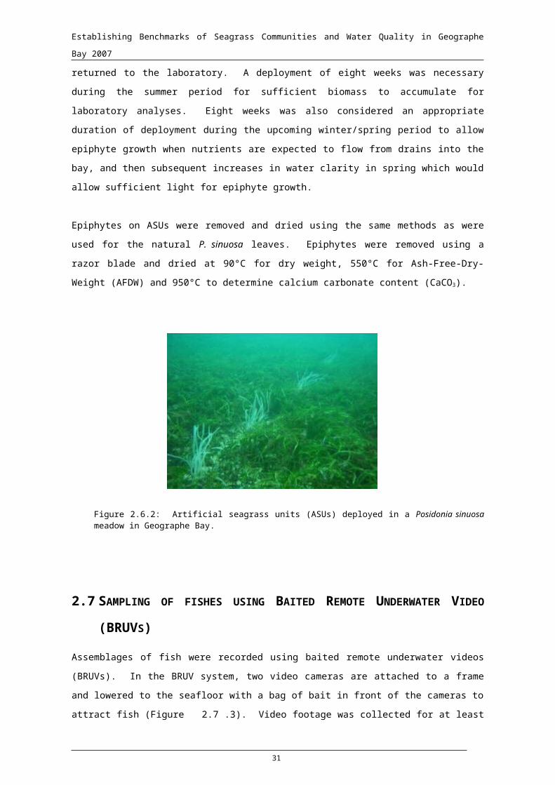
Establishing Benchmarks of Seagrass Communities and Water Quality in Geographe Bay 2007
3.2 POSIDONIA SINUOSA
3.2.1 DRAINS VERSUS NON-DRAINS – POSIDONIA SINUOSA
There were no statistically significant differences in shoot density, shoot height, biomass or leaf area index
(LAI) between drains and non-drains (Table 3.2.6 and Figure 3.2.8). There was, however, significant small
scale variability in shoot density, shoot height and LAI among the sites within each group (Table 3.2.6). In
particular, Toby Inlet had on average approximately twice the shoot density than any other site near drains.
Similarly, nearby Siesta Park had the largest shoot density on average of any of the near-shore sites. These
relative high shoot densities at Toby Inlet and Siesta Park also equated to relatively high biomass and LAIs. It
is also important to note that the morphology of leaves at Port Geographe and to a lesser extent, Forrest Beach
was relatively different from the other near-shore sites. Both sites had relatively heavy leaves compared to
LAI. For example, leaves at Port Geographe were 2-3 times the weight of leaves in the other sites when
standardised to leaf area and leaves at Forrest beach were up to twice the weight.
Figure 3.2.8: Number of shoots m-2, shoot height (cm), biomass (g.m-2 of seafloor), and leaf area index (LAI) measured in m2 of Posidonia sinuosa leaves per m2 of seafloor (mean + S.E.). For ease of comparison with other studies, data have been converted from numbers per quadrat (0.04 m2) to numbers per m2. Sites away from drains are highlighted in green and sites near drains are in red. The sites are presented in geographical order from west (Eagle Bay) to east (Forrest Beach).
31

Establishing Benchmarks of Seagrass Communities and Water Quality in Geographe Bay 2007
There were also geographical trends from west to east across Geographe Bay with shoot density on average,
highest in the western sites (Eagle Bay to Siesta Park) and shoot height increasing from west to east (Figure
3.2.8).
Table 3.2.6: Results of analyses of variance to test for differences in shoot density, shoot height, total biomass and leaf area index near to drains compared to away from drains. ns – not significant, *** - p < 0.001. a heterogeneity of variances was not removed after transformation.
Source of variation df Shoot density Shoot height Total biomass Leaf Area Index
MS F p MS F p MS F p MS
F p
Drain v Non-Drain 1 1.16 1.83 ns
127.6 0.33 ns
57.1 0.6 ns
0.012 0.64 ns
Site(D v ND) 8 0.63 4.91 ***
388.1 11.0 ***
94.6 2.1 ns
0.019 11.83 ***
Residual 50 0.13 55.2
45.5
0.002
Transform Ln(x + 1) None None Sqrt(x + 1)a
3.2.2 DISTANCE FROM SHORE – POSIDONIA SINUOSA
There were no statistically significant differences in shoot density, shoot height, biomass or leaf area index
(LAI) with distance from shore (Table 3.2.7 and Figure 3.2.9). There was, however, significant small scale
variability in shoot density, shoot height and LAI among the sites within each group (Table 3.2.7 and Figure
3.2.9). Siesta Park had on average the highest shoot density, biomass and LAI of any site in the study.
Wonnerup Beach had on average the tallest shoots.
Figure 3.2.9: Number of shoots m-2, shoot height (cm), biomass (g.m-2 of seafloor), and leaf area index (LAI) measured in m2 of Posidonia australis leaves per m2 of seafloor (mean + S.E.). For ease of comparison with other studies, data have been converted from numbers per quadrat (0.04 m2) to numbers per m2. Near-shore sites are presented in green, mid-shore sites in light blue and off-shore sites in dark blue.
32
Establishing Benchmarks of Seagrass Communities and Water Quality in Geographe Bay 2007
Table 3.2.7: Results of analyses of variance to test for differences in shoot density, shoot height, total biomass and leaf area index with distance from shore. ns – not significant, *** - p < 0.001.
Source of variation df Shoot density Shoot height Total biomass Leaf Area Index
MS F p MS F p MS F p MS F p
Distance from shore 260.1 0.09 ns
522.8 1.81 ns 136.8 2.18 ns
0.0095 1.06 ns
Site(D) 12 657.4 3.50 ***
289.3 10.39 *** 62.7 1.75 ns
0.0089 5.67 ***
Residual 75 187.7 27.9 35.9
0.0016
Transform None None None Sqrt(x + 1)
SUMMARY – POSIDONIA SINUOSA
No significant differences between drains and non-drains
Significant small scale variability among sites
Relatively high shoot density, biomass and leaf area index at Toby Inlet and Siesta Park
Tallest shoots at Wonnerup Beach
Leaves at Port Geographe 2-3 times the weight per unit area of leaf compared to other sites
No patterns of difference with distance from shore
33

Establishing Benchmarks of Seagrass Communities and Water Quality in Geographe Bay 2007
3.3 POSIDONIA SINUOSA EPIPHYTES
3.3.1 DRAINS VERSUS NON-DRAINS – POSIDONIA SINUOSA EPIPHYTES
There were no statistically significant differences in dry weight, % ash free dry weight (AFDW) or % CaCO 3
between drains and non-drains (Figure 3.3.10 and Table 3.3.9). There was, however, significant small scale
variability among the sites within each group (Table 3.3.9). In particular, dry weight of epiphytes was very
high at Eagle Bay compared to all other near-shore sites. On average, the highest % CaCO3 components were
at Wonnerup Beach and Forrest Beach.
Figure 3.3.10. Dry weight (g) of epiphytes per m2 of Posidonia sinuosa leaf, % ash free dry weight and % CaCO3
(mean +SE). Non-drain sites are presented in green and drains are in red. The sites are presented in geographical order from west (Eagle Bay) to east (Forrest Beach).
34

Establishing Benchmarks of Seagrass Communities and Water Quality in Geographe Bay 2007
Table 3.3.8: Results of analyses of variance to test for differences in dry weight, % ash free dry weight (AFDW) and % CaCO3 near to drains compared to away from drains. ns – not significant, *** - p < 0.001. a heterogeneity of variances was not removed after transformation.
Source of variation df Dry weight % AFDW % CaCO3
MS F p MS F p MS F p
Drain v Non-Drain 1 1.34 0.89 ns
405.1 3.31 ns 0.091 1.15 ns
Site(D v ND) 8 1.51 10.71 ***
122.6 6.69 *** 0.079 5.76 ***
Residual 50 0.14 18.3 0.013
Transform Ln(x + 1)a None Ln(x + 1)
3.3.2 DISTANCE FROM SHORE – POSIDONIA SINUOSA EPIPHYTES
Dry weight of epiphytes did not differ significantly with distance from shore (Figure 3.3.11 and Table 3.3.9).
There was, however, significant small scale variability among sites. This was driven largely by very high dry
weights at Eagle Bay. If Eagle Bay is excluded from the results, there is a trend of increasing average dry
weight with increasing distance from shore. Percentage ash free dry weight (AFDW) was significantly higher
in the off-shore and mid-shore compared to near-shore sites, indicating higher proportions of fleshy and
filamentous types of algae. Conversely, percentages of CaCO3 were higher in the near-shore than the mid and
off-shore indicating higher proportions of calcified types of algae.
Figure 3.3.11: Dry weight (g) of epiphytes per m2 of Posidonia sinuosa leaf, % ash free dry weight and % CaCO3
(mean +SE). Near-shore sites are presented in green, mid-shore sites in light blue and off-shore sites in dark blue.
35

Establishing Benchmarks of Seagrass Communities and Water Quality in Geographe Bay 2007
Table 3.3.9: Results of analyses of variance to test for differences in dry weight, % Ash Free Dry Weight (AFDW) and % CaCO3 with distance from shore. ns – not significant, * - p < 0.05, * - p < 0.01, *** - p < 0.001. a
heterogeneity of variances was not removed after transformation.
Source of variation df Dry weight % AFDW % CaCO3
MS
F p MS F p MS
F p
Distance from shore 2 0.48 0.20 ns 813.5 6.55 *
2244.1 10.03 **
Site(D) 12 2.40 8.92 *** 124.3 1.65 ns 223.8 2.17 *
Residual 75 0.27 75.4 103.3
Transform Sqrt(x + 1) Nonea Nonea
SNK tests Off = Mid > Near Near > Mid = Off
SUMMARY – POSIDONIA SINUOSA EPIPHYTES
No significant differences in dry weight, ash free dry weight or CaCO3 near drains compared to distant
from drains
Significant small scale variability among sites
Very high dry weight of epiphytes at Eagle Bay
When Eagle Bay is excluded from results, trend in increasing dry weight with increasing distance from
shore
% ash free dry weight higher in the off-shore and mid-shore compared to near-shore, indicating higher
proportions of fleshy and filamentous algal epiphytes.
% CaCO3 higher in near-shore compared to mid-shore and off-shore, indicating higher proportions of
calcified algal epiphytes.
36

Establishing Benchmarks of Seagrass Communities and Water Quality in Geographe Bay 2007
37
Establishing Benchmarks of Seagrass Communities and Water Quality in Geographe Bay 2007
3.4 ARTIFICIAL SEAGRASS UNITS (ASUS)
3.4.1 DRAINS VERSUS NON-DRAINS - ASUS
There were no statistically significant differences in dry weight, % ash free dry weight (AFDW) or % CaCO 3
near drains compared to away from drains (Table 3.4.10 and Figure 3.4.13). There was, however, significant
small scale variability among the sites within each group. In comparison with natural Posidonia sinuosa
plants, variability among sites was generally higher on ASUs (compare Figure 3.4.13 with Figure 3.3.10).
Figure 3.4.12: ASU showing epiphyte growth after 8 weeks in Geographe Bay.
Figure 3.4.13: Dry weight (mg) of epiphytes per cm2 of ASU, % ash free dry weight and % CaCO3. (mean +S.E.) Non-drains are presented in green and drains in red. The sites are presented in geographical order from west (Dunsborough) to east (Forrest Beach).
38

Establishing Benchmarks of Seagrass Communities and Water Quality in Geographe Bay 2007
Table 3.4.10: Results of PERMANOVA analyses to test for differences in dry weight, % ash free dry weight (AFDW) and % CaCO3 on ASUs near drains compared to away from drains. ns – not significant, *** - p < 0.001.
Source of variation df Dry weight % AFDW % CaCO3
MS Pseudo F
p MS Pseudo F
p MS Pseudo F
p
Drain v Non-Drain 1 0.0947 3.80 ns
309.24 0.437 ns
1312.2 0.64 ns
Site(D v ND) 7 0.0251 5.19 ***
711.59 16.047 ***
2059.3 10.58 ***
Residual 43
Transform None None None
3.4.2 DISTANCE FROM SHORE - ASUS
There were no statistically significant differences in dry weight, % ash free dry weight (AFDW) or % CaCO 3
with distance from shore (Figure 3.4.14 and Table 3.4.11). There was, however, significant small scale
variability among the sites within each group (Table 3.4.2).
Figure 3.4.14: Dry weight (g) of epiphytes per m2 of ASU, % ash free dry weight and % CaCO3 (mean + S.E.). Near-shore sites are presented in green, mid-shore sites in light blue and off-shore sites in dark blue.
39

Establishing Benchmarks of Seagrass Communities and Water Quality in Geographe Bay 2007
Table 3.4.11: Results of PERMANOVA analyses to test for differences in dry weight, % ash free dry weight (AFDW) and % CaCO3 on ASUs with distance from shore. ns – not significant, *** - p < 0.001.
Source of variation df Dry weight % AFDW % CaCO3
MS
Pseudo F
p MS Pseudo F
p MS
Pseudo F
p
Distance from shore 2 0.0332 0.62 ns 1154 2.73 ns 2026 1.44 ns
Site(D) 11 0.0536 7.30 *** 424 7.90 *** 1413 9.44 ***
Residual 68 0.0073 54
Transform None None None
SUMMARY – ARTIFICIAL SEAGRASS UNITS
No significant differences between drains and non-drains
No significant differences with distance from shore
Significant small-scale variability among sites
Epiphyte growth on ASUs did not show same patterns as natural Posidonia sinuosa
40
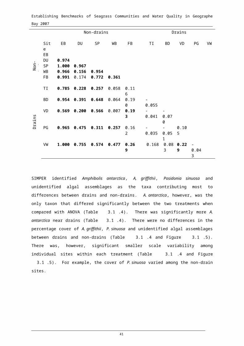
Establishing Benchmarks of Seagrass Communities and Water Quality in Geographe Bay 2007
3.5 BAITED REMOTE UNDERWATER VIDEO (BRUVS)
Seventy six species of fishes from 54 genera and 32 families were recorded on Baited Remote Underwater
Videos (BRUVS). The most abundant species were striped trumpeter (Pelates sexlineatus), yellowtail scad
(Trachurus novaezelandiae) and sand trevally (Pseudocaranx wrightii). In addition one species each of
octopus, cuttlefish, squid and crab were also recorded. Species diversity was in general highest in off-shore
sites.
Measures of species diversityHabitat Number of species Simpson Shannon-WeinerDrains near-shore 35 1.943 0.775Non-drains near-shore 36 2.331 0.859Mid-shore 35 1.888 0.706Off-shore 45 2.730 0.931
Table 3.5.12: Measures of diversity of fishes recorded in each type of habitat. Sites were pooled in each habitat type.
3.5.1 DRAINS VERSUS NON-DRAINS - BRUVS
There were no significant differences in assemblages of fishes between drain and non-drain sites when sites
were grouped together and comparisons made at large spatial scales using a nested ANOSIM (P = 11.9 %, R
= 0.128). In contrast, when comparisons were made at smaller spatial scales between individual pairs of sites,
significant differences were found using pairwise tests (Table 3.5.13 and Figure 3.5.15). On average, the sites
away from drains (green symbols) overlap to some extent with the sites near drains (red symbols). However,
when sites were examined individually, there were some clear differences in assemblages of fishes. For
example, assemblages in Eagle Bay (▲) clustered separately from assemblages in all other sites with the
exception of Dunsborough (▼) and were significantly different in ANOSIM pairwise comparisons (Table
3.5.1). Similar to the results for benthic transects, there appeared to be a slight geographic change in
assemblages of fishes across the bay. Assemblages of fish were more variable among non-drains than drain
sites as evidenced by the broader dispersion (or scatter) of the symbols representing the non-drains (green)
compared to drains (red) in Figure 3.5.15.
41

Establishing Benchmarks of Seagrass Communities and Water Quality in Geographe Bay 2007
Figure 3.5.15: MDS ordination illustrating differences in assemblages of fish in replicate Baited Remote Underwater Videos at each site. Sites away from drains are presented in green and sites near to drains are in red. Note: caution should be used in interpreting this MDS because the relatively high stress value of 0.21 suggests the ordination may be not adequately represent real patterns of difference among samples
Table 3.5.13: Summary of R values from ANOSIM comparing assemblages of fishes between pairs of sites in near-shore habitats. Bold type indicates pairs of sites that are significantly different at p < 5%. See Table 2.2.1 for explanation of abbreviations of site names.
Non-Drains Drains
Site EB DU SP WB FB TI BD VD PG VW
Non
-D
rain
s
EB - - - - - - - - - -DU 0.264 - - - - - - - - -SP 0.632 0.632 - - - - - - - -WB 0.692 0.396 0.500 - - - - - - -FB 0.754 0.374 0.376 0.250 - - - - - -
Dra
ins
TI 0.800 0.504 0.012 0.364 0.300 - - - - -BD 0.724 0.440 0.224 0.212 0.338 0.13
6- - - -
VD 0.884 0.624 0.624 0.236 0.446 0.332
0.248 - - -
PG 0.684 0.304 0.652 0.528 0.442 0.380
0.356 0.588 - -
VW 0.788 0.396 0.356 0.244 -0.076 0.168
0.328 0.372 0.172 -
SIMPER identified striped trumpeter (Pelates sexlineatus), sand trevally (Pseudocaranx wrightii), yellowtail
scad (Trachurus novaezelandiae), western gobbleguts (Apogon ruepelli), silver belly (Parequula
melbournensis) and silver trevally (Pseudocaranx dentex) as the species of fishes contributing most to
variability in assemblages among sites. There were no consistent differences in abundances between drains
and non-drains (Table 3.5.14 and Figure 3.5.16). There was, however, significant small scale variation in
abundances among sites within each group (Table 3.5.14 and Figure 3.5.16). On average there were more
western gobbleguts near drains (with the exception of Siesta Park) and in the central region of the study area
than elsewhere (Figure 3.5.16).
42

Establishing Benchmarks of Seagrass Communities and Water Quality in Geographe Bay 2007
Figure 3.5.16: Maximum numbers of trumpeter (Pelates sexlineatus), sand trevally (Pseudocaranx wrightii), yellowtail scad (Trachurus novaezelandiae), gobbleguts (Apogon ruepellii), silver belly (Parequula melbournensis) and silver trevally (P. dentex) observed with Baited Remote Underwater Videos (BRUVS) in near-shore sites. Non-drain sites are highlighted in green and drain sites are in red. The sites are presented in geographical order from west (Eagle Bay) to east (Forrest Beach).
43

Establishing Benchmarks of Seagrass Communities and Water Quality in Geographe Bay 2007
Table 3.5.14: Results of analyses of variance to test for differences in Maximum Number of striped trumpeter, sand trevally, yellowtail scad, western gobbleguts, silver belly and silver trevally in sites near drains compared to sites away from drains. ns – not significant, * - p < 0.01, ** - p < 0.01, *** - p < 0.001. a heterogeneity of variances was not removed after transformation.
Source of variation df Striped trumpeter
Sand trevally Yellowtail scad
MS F p MS F p MS F p
Drain v Non-Drain 1 7.81 2.43 ns 0.21 0.04 ns
1.06 0.29 ns
Site(D v ND) 8 3.23 2.51 * 4.83 3.70 **
3.68 2.18 ns
Residual 40 1.28 1.31
1.69
Transform Ln(x + 1) Ln(x + 1)a Ln(x + 1)
Source of variation df Western gobbleguts
Silver belly Silver trevally
MS F p MS F p MS F p
Drain v Non-Drain 1 3.34 1.8 ns 0.01 0.01 ns
4.54 2.33 ns
Site(D v ND) 8 1.85 7.63 *** 1.21 1.71 ns
1.95 9.81 ***
Residual 40 0.24 0.71
0.20
Transform Ln(x + 1)a Ln(x + 1)a Ln(x + 1)a
3.5.2 DISTANCE FROM SHORE - BRUVS
Assemblages of fishes differed significantly with distance from shore (nested ANOSIM: R = 0.464, p = 0.1
%). Pairwise comparisons revealed the near-shore habitat to be significantly different from both mid
(ANOSIM: R = 0.544, p = 0.8 %) and off-shore (ANOSIM: R = 0.616, p = 0.8%). There was also a
significant difference between mid and off-shore habitats (ANOSIM: R = 0.316, p = 4.8 %), although this was
weaker than comparisons with the near-shore. These results are clearly illustrated in where the near-shore
sites (green symbols) group separately from the mid (light blue symbols) and off-shore (dark blue symbols)
sites. The nested ANOSIM also identified significant smaller scale variation among the individual sites
nested within each of the distances from shore (nested ANOSIM: R = 0.394, p = 0.1%)
44

Establishing Benchmarks of Seagrass Communities and Water Quality in Geographe Bay 2007
Figure 3.5.17: MDS ordination illustrating differences in assemblages in assemblages of fish in replicate Baited Remote Underwater Videos. Near-shore sites are presented in green, mid-shore sites in light blue and off-shore sites in dark blue.
Striped trumpeter (Pelates sexlineatus) were most abundant in near-shore habitats, while western king
wrasse (Coris auricularis) and maori wrasse (Ophthalmolepis lineolatus) were most abundant in the off-
shore habitats (Table 3.5.15 and Figure 3.5.18). Abundances of striped trumpeter, silver belly (Parequula
melbournensis), sand trevally (Pseudocaranx wrightii), silver trevally (P. dentex), western king wrasse
(Coris auricularis), maori wrasse and black headed puller (Chromis klunzingeri) varied significantly at
smaller scales among sites (Table 3.5.15 and Figure 3.5.18). There was also a trend of decreasing
abundance of western king wrasse, a reef associated wrasse, with increasing distance from Cape Naturaliste
(Figure 3.5.18).
45

Establishing Benchmarks of Seagrass Communities and Water Quality in Geographe Bay 2007
Table 3.5.15: Results of analyses of variance to test for differences with distance from shore in Maximum Numbers of striped trumpeter, silver belly, sand trevally, yellowtail scad, silver trevally, Notolabrus parilus, western king wrasse, Maori wrasse and black headed puller counted in BRUVs. ns – not significant, * - p < 0.05, ** - p < 0.01, *** - p < 0.001. a heterogeneity of variances was not removed after transformation.
Source of variation
df Striped trumpeter
Silver belly Sand trevally Yellowtail scad Silver trevally
MS F p MS F p MS
F p MS F p MS F p
Distance from Shore
2 23.92 15.8 *** 3.68 2.3 ns 2.49 1.1 ns 1.56 1.0 ns 3.43 1.4 ns
Site(D) 121.52 2.6 ** 1.60 4.5 ***
2.28 3.3 *** 1.53 1.5 ns 2.37 4.1 ***
Residual 600.60
0.36
0.68 1.03 0.58
Transform Ln(x + 1)a Ln(x + 1) Ln(x + 1)a Ln(x + 1)a Ln(x + 1)
SNK tests Near >> Mid = Off
Source of variation df Orange spotted wrasse
Western king wrasse
Maori wrasse Black headed puller
MS F p MS F p MS F p MS F p
Distance from shore 1 0.33 0.20 ns 5.33 4.50 * 8.29 7.33 ** 1.87 1.22 nsSite(D) 8 1.63 1.76 ns 1.18 7.35 *** 1.13 9.56 *** 1.54 3.08 **Residual 50 0.93 0.16 0.12 0.50
Transform None Sqrt(x + 1)a Ln(x + 1) Ln(x + 1)a
SNK tests Off > Mid = Near
Off > Mid = Near
46
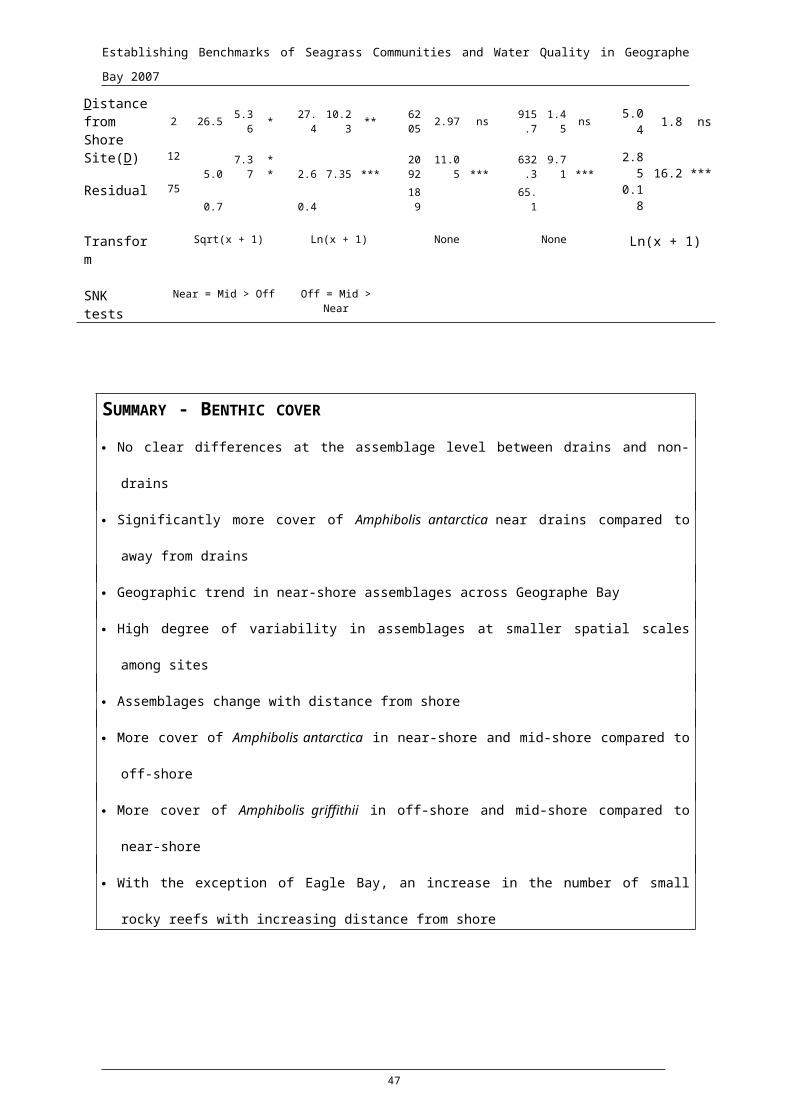
Establishing Benchmarks of Seagrass Communities and Water Quality in Geographe Bay 2007
Figure 3.5.18: Maximum numbers of striped trumpeter (Pelates sexlineatus), silver belly (Parequula melbournensis), yellowtail scad (Trachurus novaezelandiae), silver trevally (Pseudocaranx. dentex), orange spotted wrasse (Notolabrus parilus), western king wrasse (Coris auricularis), maori wrasse (Ophthalmolepis lineolatus) and black headed puller (Chromis klunzingeri) counted in BRUVs. Near-shore sites are presented in green, mid-shore sites in light blue and off-shore sites in dark blue.
47

Establishing Benchmarks of Seagrass Communities and Water Quality in Geographe Bay 2007
Maori wrasse (Ophthalmolepis lineolatus) Western king wrasse (Coris auricularis)
Yellowtail scad (Trachurus novaezelandiae) Silver belly (Parequula melbournensis)
Western gobbleguts (Apogon ruepelli) Striped trumpeter (Pelates sexlineatus)
Orange spotted wrasse (Notolabrus parilus) - male White trevally (Pseudocaranx dentex)
Figure 3.5.19: Examples of fishes observed in Baited Remote Underwater Videos.
48

Establishing Benchmarks of Seagrass Communities and Water Quality in Geographe Bay 2007
SUMMARY - BAITED REMOTE UNDERWATER VIDEO OF FISHES
Seventy six species of fish, from 52 genera and 32 families
Highest diversity at off-shore sites followed by near-shore non-drain sites
One species each of octopus, cuttlefish, squid and crab
No differences in assemblages nor species abundances between drains and non-drains
Significant small-scale variation in assemblages and abundances among sites
Significant differences in assemblages with distance from shore
Striped trumpeter (Pelates sexlineatus) most abundant in near-shore habitats
Western king wrasse (Coris auricularis) and maori wrasse (Ophthalmolepis lineolatus) most abundant in
off-shore sites
49

Establishing Benchmarks of Seagrass Communities and Water Quality in Geographe Bay 2007
3.6 NON-CRYPTIC MOBILE AND SESSILE BENTHIC INVERTEBRATES
Formal statistical analyses are yet to be done for invertebrates because many of the species are still in the
process of being identified. These will be included in the 2007-08 report. Preliminary examination of the
data, however, suggests many of the taxa have extremely patch distributions (i.e. were not widespread and
only found in one or a small number of sites).
3.6.1 CORALS AND ZOANTHIDS
All 5 species of corals were uncommon and/or extremely patchily distributed. Four of the 5 species were
represented by 1 or 2 specimens. Only Coral species # 4 was relatively abundant, but only occurred at a
single site, Wonnerup Beach, with an average abundance of 6 colonies per transect. Abundances and
diversity were likely to have been higher if rocky reefs, where corals commonly occur, had been sampled but
inclusion of this additional habitat was beyond the scope of this project.
Coral species # 1 Coral species # 2
Coral species # 4 – dark green circles Zoanthid – Isaurus cliftoni
Figure 3.6.20: Examples of corals found in Geographic Bay.
50

Establishing Benchmarks of Seagrass Communities and Water Quality in Geographe Bay 2007
3.6.2 ECHINODERMS (SEA STARS, SEA URCHINS AND SEA CUCUMBERS)
Seven species of sea star, one sea urchin and one sea cucumber were recorded in transects. Most were
uncommon and represented by only a few individuals across the sampling sites, with the exception of the sea
star, Patiriella brevispina. This species was relatively abundant towards the north of the study area in the
Vasse Wonnerup and Wonnerup Beach Sites, with an average abundance of 31 individuals per transect.
Sea star - Nepanthia crassa Sea star - Fromia polypora
Sea star - Archaster angulatus Sea star - Pentagonaster dubeni
Sea star - Tosia australis Sea star - Patiriella brevispina
Sea urchin - Amblypneustes leucoglobus Sea cucumber - Stichopus mollis
Figure 3.6.21: Examples of echinoderms found in Geographe Bay
51
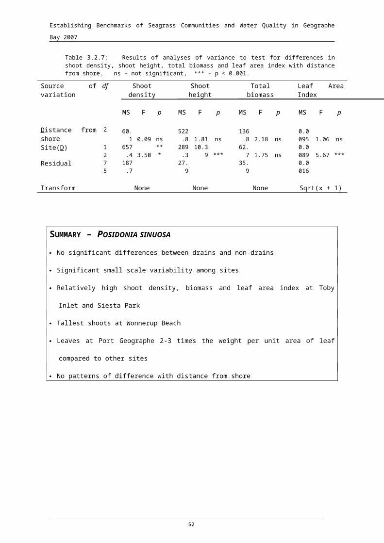
Establishing Benchmarks of Seagrass Communities and Water Quality in Geographe Bay 2007
3.6.3 ASCIDIANS (SEA SQUIRTS)
Twelve species of ascidians were recorded in transects. These included several species of colonial ascidian.
Colonial ascidians are relatively small and form colonies of thousands of individuals. They often colonise the
leaves of seagrasses being tightly grouped and forming intricate patterns (see Botryllus schlosseri in Figure
3.6.22). Several species of solitary ascidian were also recorded. Solitary ascidians are typically larger than
colonial ascidians and individuals in this study were found both growing attached to seagrasses and on the
sediment.
Colonial ascidian – Clavelina molluccensis Solitary ascidian – Polycarpa viridis
Colonial ascidian – Botryllus schlosseri Colonial ascidian – Botryllus schlosseri
Figure 3.6.22: Examples of ascidians found in Geographe Bay.
52
Establishing Benchmarks of Seagrass Communities and Water Quality in Geographe Bay 2007
3.6.4 SPONGES
Seventy two sponge specimens were collected for identification. Final identifications will be done by the
Western Australian Museum, but preliminary examinations suggest there may be 40-60 species. Many
appeared to be extremely patchy with restricted distributions, while others were more common and
widespread. They had a variety of growth and colour forms (Figure 3.6.23) and were found growing attached
to seagrasses, in the sediment and attached to small pieces of hard substrata. Because sampling was designed
to target seagrasses only and to avoid patches of rocky reef, the diversity and abundances of sponges is almost
certainly an underestimate for the total diversity in Geographe Bay.
Figure 3.6.23: Examples of sponges found in Geographe Bay. Species are to be identified by the Western Australian Museum.
53

Establishing Benchmarks of Seagrass Communities and Water Quality in Geographe Bay 2007
3.6.5 MOLLUSCS
Only two large molluscs were recorded in transects. The large bivalve mollusc, Pinna bicolor was found at 5
of the 12 sites sampled (Siesta Park, Vasse Wonnerup, MS1, MS2 and OS6), but only in low abundances of 1
or 2 per site. The gastropod (marine snail), Campanile symbolicum was found at two sites (Dunsborough and
Wonnerup Beach), but again only in low abundances of 1 or 2 per transect.
SUMMARY - INVERTEBRATES
Five species of coral and one zoanthid
Seven species of sea star, one sea urchin and one sea cucumber
Twelve species of ascidians
Seventy two sponge specimens collected – identifications to be done by the Western Australian Museum
Two large molluscs – the bivalve, Pinna bicolor and the marine snail, Campanile symbolicum
Preliminary examination of the data suggest very patchy distributions for many of the species and
relatively few species that are widespread
Some sponge species may be new to science
3.7 WATER QUALITY – MARCH 2007
Water quality measurements are presented in Table 3.7.16 and comparisons made with other studies in Figure
3.7.24. Temperature ranged from 20.6 to 23.9 °C. At most sites there was little to no difference in surface
compared to bottom temperatures, with the exception of mid-shore sites 4 and 5 and off-shore site 4 where
bottom temperatures were 1.2 – 1.7 °C cooler. Salinity ranged from 34.5 to 35.1 ‰ (i.e. parts per thousand).
Overall, waters tended to be well mixed with little evidence for stratification. There was a very small trend of
decreasing salinity with distance from shore with near-shore sites on average 0.2 ‰ saltier than mid and off-
shore sites. Turbidity was generally low across the bay with good water clarity and only small differences
among sites. Dissolved oxygen (%) ranged from 97.4 to 115.6 and was within the normal limits of healthy
systems. Chlorophyll a concentrations were generally low, ranging from 0.2 to 0.8 μgL-1 and below the trigger
values set in ANZECC guidelines (ANZECC, 2000).
Nitrate and nitrite, orthophosphate, and total phosphorous concentrations were generally low, close to or
below levels of detection and below ANZECC trigger values. In contrast, ammonia concentrations were
above ANZECC trigger values in several sites, particularly in the near-shore (Eagle Bay, Toby Inlet, Siesta
Park, Buayanup drain, Vasse Diversion Drain, Vasse Wonnerup, Wonnerup Beach, Mid-shore site 1 and Mid-
shore site 5).
In comparison with previous surveys of water quality in Geographe Bay, most concentrations of nutrients and
chlorophyll were similar or lower, with the exception of ammonia concentrations which were relatively higher
than previous years particularly at Toby Inlet and Buayanup Drain. Compared to another large Western
Australian coastal bay (Warnbro Sound), nutrients concentrations were generally lower, but at this stage of
54

Establishing Benchmarks of Seagrass Communities and Water Quality in Geographe Bay 2007
the study these comparisons are preliminary and should be interpreted with caution. Because they include
only one sampling period in March 2007, comparisons between years could potentially be confounded by
shorter-term fluctuations in water quality. As the current study proceeds and more measurements of water
quality are recorded, it will be possible to make comparisons among years with more confidence.
Concentrations in winter are also likely to be higher when drains and river are flowing and discharging to
Geographe Bay.
Figure 3.7.24: Comparisons of nutrient and chlorophyll a concentrations sampled in the current study (red or green bars) with data collected in comparable sites in 1994 by McMahon and Walker (1997) (open bars) and in 2002 by Sinclair Knight and Merz (2003) (grey bars). Dashed lines represent ‘trigger’ values set by the Australian and New Zealand Environmental Conservation Council and solid lines represent concentrations recorded in Warnbro Sound (DEP (WA), 1996). * indicates concentrations were below limits of detection.
The two methods trialled for measuring light intensity (Licor PAR sensor and Secchi Disc) proved to be
unreliable because variable cloud cover and sea conditions caused large short-term fluctuations in readings
and therefore confounded comparisons among sites. Longer-term monitoring, where light loggers are secured
to the seafloor for a number of days, will be implemented in August and October 2007 and again in Jan - Mar
2008. Longer-term measurements will overcome such problems by averaging out short-term fluctuations over
longer periods of time.
55

Establishing Benchmarks of Seagrass Communities and Water Quality in Geographe Bay 2007
Table 3.7.16: Measurements of water quality recorded in Geographe Bay in March 2007.
Site
Dat
e sa
mpl
ed
Posi
tion
in w
ater
col
umn
Dep
th (m
)
Tem
pera
ture
(°C
)
Salin
ity (‰
)
pH
Dis
solv
ed o
xyge
n (%
)
Tur
bidi
ty (n
tu)
Am
mon
ia (µ
g.N
/L)
Ort
ho p
hosp
hate
(µ
g.P/
L)
Nitr
ate
and
nitr
ite
(µg.
N/L
)
Tot
al p
hosp
horo
us
(µg.
P/L
)
Tot
al n
itrog
en (µ
g.N
/L)
Chl
orop
hyll
a (µ
g/L
)
Eagle Bay 27/03/2007 Bottom 9.3 20.6 34.9 8.49 99.4 no data <3 4 <2 <5 80 0.8Eagle Bay 27/03/2007 Surface 1.0 20.6 34.8 8.8 101.1 no data 7 <2 <2 <5 90 0.8Dunsborough 22/03/2007 Bottom 4.9 21.7 34.6 9.1 103.2 0.65 5 3 <2 <5 100 0.4Dunsborough 22/03/2007 Surface 1.1 21.7 34.5 9.03 103.0 0.49 5 4 2 <5 100 0.5Toby Inlet 9/03/2007 Bottom 2.5 22.9 34.9 9.12 101.9 1.62 12 2 <2 <5 160 0.3Toby inlet 9/03/2007 Surface 0.8 22.9 34.9 9.12 102.0 1.80 8 2 <2 5 140 0.3Siesta Park 9/03/2007 Bottom 3.0 22.8 34.9 9.11 98.1 2.48 9 <2 <2 <5 120 0.3Siesta Park 9/03/2007 Surface 1.0 22.8 35.0 9.11 98.0 2.03 7 2 2 <5 120 0.4Buayanup 9/03/2007 Bottom 2.5 22.8 35.0 9.13 101.1 2.52 10 3 <2 <5 120 0.3Buayanup 9/03/2007 Surface 1.0 22.8 35.0 9.13 101.2 0.93 9 3 <2 <5 100 0.3Vasse Div Drain 22/03/2007 Bottom 2.4 22.2 35.2 9.16 108.9 0.66 6 3 <2 <5 120 0.3Vasse Div Drain 22/03/2007 Surface 1.0 22.2 35.2 9.16 108.9 0.62 <3 3 <2 <5 100 0.3Port Geographe 8/03/2007 Bottom 4.8 22.7 34.8 9.18 111.3 0.63 <3 <2 <2 <5 100 0.5Port Geographe 8/03/2007 Surface 0.7 22.8 34.7 9.11 110.4 1.06 5 2 <2 <5 100 0.5Vasse Wonnerup 8/03/2007 Bottom 4.2 22.9 34.8 9.27 115.6 1.05 5 <2 <2 8 130 0.4Vasse Wonnerup 8/03/2007 Surface 0.9 23.2 34.9 9.22 111.1 1.02 8 <2 <2 <5 140 0.5Wonnerup Beach 8/03/2007 Bottom 4.4 23.2 35.1 9.22 111.7 0.92 5 <2 <2 <5 140 0.6Wonnerup Beach 8/03/2007 Surface 1.1 23.7 35.1 9.16 106.6 0.49 7 2 <2 5 160 0.4Forrest Beach 8/03/2007 Bottom 3.2 23.2 35.0 9.2 113.2 2.57 <3 3 <2 <5 120 0.8Forrest Beach 8/03/2007 Surface 0.6 23.5 34.7 9.15 105.4 1.15 4 3 <2 <5 140 0.6MS1 22/03/2007 Bottom 9.7 21.6 34.7 9.06 100.5 0.70 8 4 <2 <5 150 0.5MS1 22/03/2007 Surface 1.1 21.6 34.6 9.05 101.1 0.59 7 4 <2 7 350 0.4MS2 9/03/2007 Bottom 7.8 22.2 34.8 9.13 105.9 1.97 4 <2 <2 <5 100 0.2MS2 9/03/2007 Surface 0.9 22.2 34.7 9.11 106.5 5.50 <3 <2 <2 8 90 0.2MS3 9/03/2007 Bottom 8.4 22.2 34.8 9.14 104.5 no data 3 3 <2 <5 100 0.2MS3 9/03/2007 Surface 1.0 22.2 34.8 9.13 106.0 no data <3 <2 <2 <5 110 0.2MS4 8/03/2007 Bottom 9.5 22.1 34.6 9.22 114.3 0.51 5 <2 <2 <5 90 0.3MS4 8/03/2007 Surface 0.7 23.3 34.7 9.19 108.8 0.48 <3 3 <2 <5 100 0.3MS5 8/03/2007 Bottom 9.5 22.2 34.6 9.21 107.9 4.30 3 4 <2 <5 100 0.4MS5 8/03/2007 Surface 1.0 23.9 34.8 9.19 106.6 0.67 11 3 <2 <5 120 0.3OS1 22/03/2007 Bottom 17.9 21.5 34.7 9.04 97.4 0.48 <3 3 <2 <5 120 0.4OS1 22/03/2007 Surface 1.0 21.5 34.7 9.03 100.0 0.50 <3 4 <2 <5 190 0.4OS2 22/03/2007 Bottom 15.7 21.7 34.9 9.06 98.5 1.42 4 4 <2 <5 100 0.3OS2 22/03/2007 Surface 1.1 21.7 34.8 9.06 100.9 0.76 <3 4 <2 7 280 0.3OS3 22/03/2007 Bottom 16.0 21.6 34.8 9.06 99.6 0.40 5 8 <2 <5 80 0.3OS3 22/03/2007 Surface 1.0 21.6 34.9 9.05 101.7 0.44 5 3 <2 <5 190 0.3OS4 8/03/2007 Bottom 16.0 21.9 34.5 9.17 106.9 3.85 <3 2 <2 <5 100 0.3OS4 8/03/2007 Surface 1.0 23.0 34.6 9.13 103.5 0.70 <3 3 <2 <5 90 0.2OS5 9/03/2007 Bottom 14.9 22.0 34.8 9.12 99.2 0.44 4 <2 <2 <5 90 0.3OS5 9/03/2007 Surface 1.0 22.0 34.8 9.11 102.0 0.76 5 2 <2 <5 100 0.3
Limits of readings for nutrient and chlorophyll measurements <3 <2 <2 <5 <50 <0.1
56
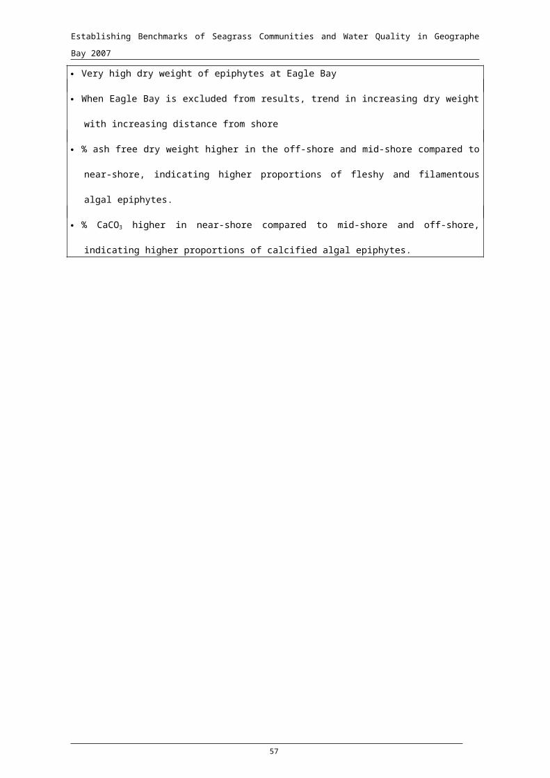
Establishing Benchmarks of Seagrass Communities and Water Quality in Geographe Bay 2007
SUMMARY – WATER QUALITY – MARCH 2007 Turbidity generally low in summer – autumn period
Ammonia concentrations above ANZECC trigger values in several near-shore and 2 mid-shore sites
Concentrations of remaining nutrients generally low and below ANZECC trigger values
Chlorophyll a concentrations generally low and below ANZECC trigger values
In general, few indications of poor water quality but winter sampling necessary to evaluate effect of drains
on water quality.
57

Establishing Benchmarks of Seagrass Communities and Water Quality in Geographe Bay 2007
4 DISCUSSION
This study quantified patterns of distribution of seagrasses, fish, epiphytes and non-cryptic invertebrates as
well as measuring water quality in the seagrass dominated habitats of Geographe Bay in the summer/autumn
of 2006/07. This study represents the first broad-scale study of Geographe Bay that includes the deeper
seagrass meadows (see (Lord and Associates, 1995; McMahon et al., 1997; McMahon et al., 1998; SKM,
2003) for previous studies in the near-shore habitats).
Although there were few significant differences between drains and non-drains when sites were grouped
together, there are several reasons why it cannot be assumed there are no impacts from drains. Impacts may
be occurring at spatial and/or temporal scales not examined in this part of the study. One of the key findings
of this study was the large spatial variability among sites in almost all the variables examined. Not all drains
are similar and likely differ in their flows and nutrient inputs into the bay. Therefore, the type, spatial extent
and organisms affected may vary among individual drains. For example, relatively high shoot densities and
biomass of Posidonia sinuosa at Toby Inlet may indicate an impact, but if the impact is specific only to that
drain then it may be averaged out or ‘hidden’ among the data for the other drain sites which are not impacted
in the same way. Similarly, P. sinuosa leaves were relatively heavy at Port Geographe compared to other
sites, which again may indicate an impact specific to that drain, but was not identified in statistical tests
because the pattern was not consistent among the drains. The detection of impacts at specific drains is likely
to be valuable for the management of Geographe Bay because it may allow targeted control of specific
impacts in catchments or targeted repair within Geographe Bay itself. For impacts to be detected at these
smaller spatial scales, differences in communities caused by an impact must be differentiated from natural
background variability. Because this study identified large background variability among sites, future
sampling designs to detect small-scale impacts will include increased replication at the scale of site. For
example, a sampling design appropriate to detect an impact at a specific drain could include multiple sites
near to the drain (e.g. 2 – 3 replicate sites 100s m apart in close proximity to the drain) compared to multiple
groups of the same configuration of sites distant from the drain (see (Underwood, 1992; Underwood, 1994)
for logic of including multiple control sites in environmental impact studies). An alternative sampling design
may include a gradient of sites leading away from the drain.
Conversely, some impacts may be occurring at spatial-scales larger than those examined in the present study
(i.e. encompassing the entire or large parts of the study area). A key component measuring large-scale
changes is tracking changes through time. The present study represents the first step in this process by
identifying benchmarks of natural community structure and water quality on which future changes can be
assessed. However, as stated at the inception of the project, at least five years of data would be desirable to
gain an understanding of inter annual (or among year) differences that may result from changes in the
Leeuwin current, El Nino events, climate change or other unforeseen influences.
Further, responses of marine communities to environmental impacts may be only transient and detectable at
certain times. For example, high flows of nutrient laden and turbid water from drains during winter may have
short-term effects on marine communities from which they recover over summer. Such impacts would not
have been detected over the summer/autumn sampling period. Sampling of water quality and epiphytes on
58
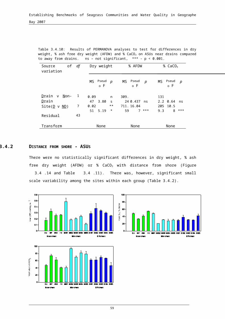
Establishing Benchmarks of Seagrass Communities and Water Quality in Geographe Bay 2007
ASUs is, however, planned for August/September to coincide with periods of high flow from drains when
impacts are likely to occur.
4.1.1 BENTHIC COVER
Seagrass cover in Geographe Bay appears to have remained relatively stable in recent years with average
cover per site estimated to be 69 ± 6.1 %, compared to similar estimates of 76-78 % taken from 2004 aerial
photos (GEM, 2007). In contrast to Lord and Associates (1995) who reported seagrasses to become ‘sparse
and patchy’ below 14 m depth of water, in the present study seagrass cover (dominated by Amphibolis
griffithii and Posidonia sinuosa) was estimated at 50 - 60 % in the off-shore sites (15 – 20 m depth).
This study identified a number of important patterns in benthic assemblages in Geographe Bay. In the near-
shore sites there was a geographic trend across the Bay driven by relatively high and consistent cover of
Amphibolis antarctica in the central region from Buayanup Drain to Wonnerup Beach compared to relatively
lower cover towards the western and eastern ends of the study area (Figure 3.1.5). Although this pattern was
correlated with the position of the drains, it is difficult to determine whether it is an impact of proximity to the
drains or simply a natural pattern of distribution across the Bay. For example, Searle (1977) suggested that
seagrass distribution in Geographe Bay may be driven by patterns of hydrology and sediment deposition.
There were also clear changes with increasing distance from shore with the cover of the seagrasses, A.
antarctica and P. sinuosa decreasing, and A. griffithii and the number of rocky reefs increasing (see Figure
3.1.7). The changes in seagrass species composition were also correlated with increasing depth of water and
are typical of other seagrass meadows in the region. It is very likely that increases in the number of rocky
reefs with distance from shore have important ecological influences on assemblages of fishes, invertebrates
and algal assemblages. The presence of small rocky reefs is typical within seagrass meadows along the
southern Western Australian coast (Cambridge et al., 2000) and are often associated with the position of
previous shorelines when sea levels were lower. Numerous studies have highlighted the importance of the
presence and proximity of hard substrata in structuring fish assemblages (Howard, 1989; Ayvazian et al.,
1995; Friedlander et al., 1998; Chittaro, 2004; Wernberg et al., 2006). The small rocky reefs in Geographe
Bay may also provide source populations of organisms which can then move into or colonise the surrounding
seagrasses. For example, organisms such as sponges which may have source populations on rocky reefs, often
have short larval dispersal distances (i.e. only swim or crawl short distances or remain for only short periods
of time in the plankton before settling), and therefore may only colonise short distances into the surrounding
seagrasses (Farnsworth et al., 1996). Similarly, Van Elven et al. (2004) suggested that high diversity of
epiphytic algae in seagrass meadows was attributed to proximity to reefs. Overall, it is likely the presence of
rocky reefs will influence the fish, invertebrate and algal assemblages within the surrounding seagrass
meadows. It is important, therefore, to consider the presence of rocky reefs when interpreting differences in
assemblages of organisms among sites.
Finally, there was significant small-scale spatial variability among sites for almost all the variables examined.
As discussed above, high variability among sites can complicate comparisons made at larger spatial scales
(e.g. drains versus non-drains) and must be considered for future sampling designs.
59
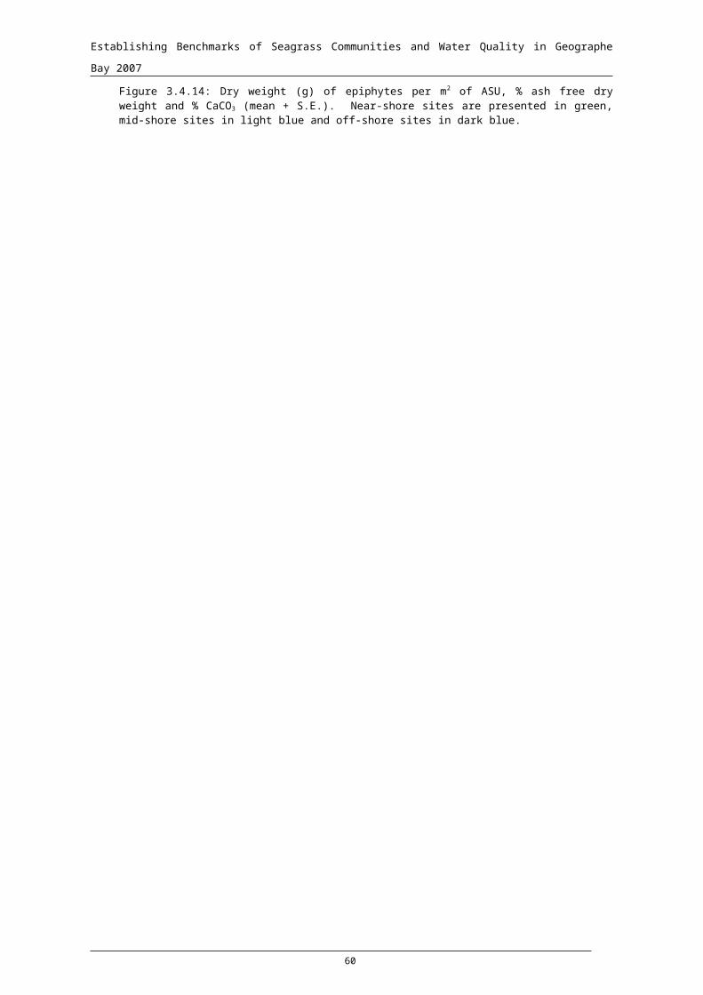
Establishing Benchmarks of Seagrass Communities and Water Quality in Geographe Bay 2007
4.1.2 POSIDONIA SINUOSA
Comparisons with other studies suggest the biomass of Posidonia sinuosa meadows have not changed
dramatically in the Bay in recent years. For example, in this study the above ground biomass of Posidonia
sinuosa (157 to 535 gm-2) was similar to that reported by McMahon et al. (1997) for Geographe Bay in the
summers of 1993/94 and 1994/95 (115 to 470 gm-2). Further, McMahon et al. (1997) suggested these values
were similar to other unpolluted systems in southern Australia.
Two patterns of P. sinuosa growth were indicative of potential environmental impacts. First, shoot density
and biomass were on average relatively high at Toby Inlet and Siesta Park compared to all other sites in the
Bay including mid and off-shore sites (Figure 3.2.8 and Figure 3.2.9). High shoot density and biomass may
be indicative of localised high nutrient levels. Second, P. sinuosa leaves at Port Geographe and Forrest Beach
were relatively heavy compared to other sites in terms of weight to leaf area. Again, these results may be
indicative of high nutrient levels or slow growing plants. It is, however, difficult to attribute these patterns to
an impact from the drain. More targeted assessments of these drains would be needed to better understand
(see above).
4.1.3 EPIPHYTES ON POSIDONIA SINUOSA
There were no patterns in epiphyte loads to suggest an impact of drains in the near-shore. There were,
however, very high loads on Posidonia sinuosa leaves at Eagle Bay. The most likely explanation for high
loads in Eagle Bay is the large number and proximity of rocky reefs (Van Elven et al., 2004).
In contrast, there were clear patterns of difference with distance from shore. If Eagle Bay is excluded from
the analyses, there is an increase in epiphyte dry weight and ash free dry weight (AFDW) with distance from
shore and a corresponding decrease in CaCO3. While high % AFDW compared to % CaCO3 may indicate
more nutrient rich environments, it is unlikely to be the case in Geographe Bay. Rather, larger epiphyte loads
and AFDW in mid and off-shore sites may be a result of reduced mechanical disturbance. Because these sites
are in deeper water than near-shore sites there is likely to be less wave action to remove epiphytes.
4.1.4 ARTIFICIAL SEAGRASS UNITS (ASUS)
Similar to patterns of epiphyte growth on natural Posidonia sinuosa leaves, there was no evidence to suggest
impacts of drains on ASU epiphytes during summer/autumn 2007. In contrast to P. sinuosa, however, there
were no differences with distance from shore. This may have been a result of the length of time for epiphyte
colonisation and growth. Natural P. sinuosa leaves live for up to 210 day in Geographe Bay (Marba et al.,
1999) compared to the 56 days the ASUs were deployed.
4.1.5 BAITED REMOTE UNDERWATER VIDEO (BRUVS)
With the exception of the work done by Scott (1981), there are relatively few quantitative studies of the whole
fish assemblages of Geographe Bay on which to compare with the present study. The present study recorded
76 species of fishes compared to the 19 reported by Scott (1981). The increase is almost certainly a result of
different sampling techniques and sites rather than a real change in diversity. Scott (1981) used a relatively
60

Establishing Benchmarks of Seagrass Communities and Water Quality in Geographe Bay 2007
small beam trawl, which would have been unlikely to sample many of the larger and faster moving fishes
recorded in BRUVS. In addition, Scott (1981) only sampled near-shore seagrass meadows and would not
have encountered some of the species recorded by BRUVs in deeper sites. While Scott (1981) provided
important data, the much larger number of species recorded in the present study highlights the need to use
appropriate techniques and adequate replication to achieve more accurate estimates of fish diversity in the
seagrass meadows of Geographe Bay.
Other studies have included sites at Geographe Bay as part of larger assessments of a subset of fishes(Hyndes
et al., 1999; Platell et al., 2001). These have used beam trawl nets which may not capture the range of fishes
recorded using non destructive techniques such as baited remote underwater video used in this study.
Species heavily targeted by fishers, such as samson fish (5 individuals), break sea cod (1 individual), pink
snapper (3 individuals) and harlequin fish (1 individual) were relatively uncommon in BRUVs.
For several species, there were clear patterns of increased abundance with the presence or proximity to rocky
reefs. For example, maori wrasse were most abundant in mid and off-shore sites where rocky reefs were
present and were only present in the near-shore at Eagle Bay which also had many reefs. Similarly, western
king wrasse and black headed puller were most abundant in the western sites closer to the substantial rocky
reefs associated with Cape Naturaliste.
4.1.6 NON-CRYPTIC SESSILE AND MOBILE INVERTEBRATES
Final analyses of invertebrate data will be included in the 2007-08 report once identifications have been done
by the Western Australian Museum. However, preliminary analyses suggest sea stars, urchins and sea
cucumbers were typical of temperate seagrass meadows (Coleman, 2007). In addition, sponge assemblages
appear relatively diverse compared to those in other temperate Australian seagrass habitats. For example, it
is likely that more than 30 species of sponges were found in this survey, compared to nine species found by
Barnes et al. (2006) in New South Wales seagrass meadows using similar methods and sampling intensities.
4.1.7 WATER QUALITY
Because the data represent the first time of sampling only and summer / autumn only, they should be
interpreted with caution. Nevertheless, water quality in Geographe Bay could generally be considered good
during autumn 2007. However, ammonium concentrations were above the ANZECC trigger values at several
of the near-shore sites. The fact that levels were high at both drain and non-drain sites, suggests that if the
high concentrations are coming from the land, they are either coming via the drains and mixing with oceanic
water, or alternatively through the flow of groundwater.
61
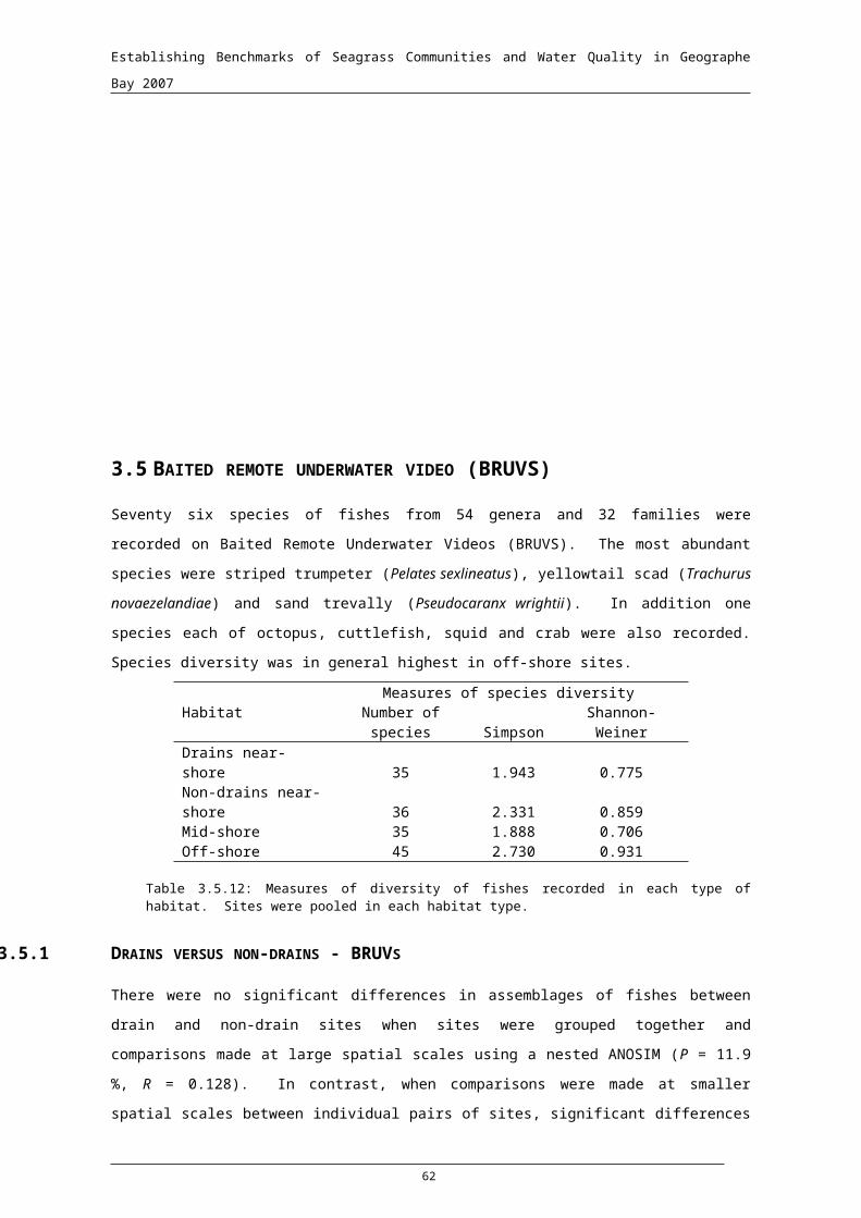
Establishing Benchmarks of Seagrass Communities and Water Quality in Geographe Bay 2007
4.2 PROJECT OUTCOMES
As outlined in the project application, this study has produced the following outcomes:
a set of data describing patterns of distribution and abundance of benthic habitats, seagrasses,
epiphytes, fishes, invertebrates and water quality from which future impacts or changes can be
detected (however, longer term monitoring is needed to understand natural patterns of temporal
variability);
the first comprehensive and simultaneous sampling of seagrass meadows, their associated fauna and
water quality, for a range of depths and locations throughout Geographe Bay; and
the first year of data from which resource condition targets (RCTs) can be developed for the long term
management of Geographe Bay. RCTs will be developed as more data become available, particularly
the winter / spring sampling and repeated summer / autumn sampling. RCTs are likely to be
developed based on: values of epiphyte biomass on artificial seagrasses, changes in the diversity of
fish or invertebrate assemblages, changes in characteristics of seagrass growth such as shoot density,
biomass or leaf area and changes in water quality.
It must be noted that this study was not designed to test for small scale impacts of individual drains. Rather, it
provides a comprehensive assessment of broadscale patterns in seagrass communities from representative
sites throughout Geographe Bay and the necessary information to design more intensive and targeted
assessments for specific areas which show signs of potential environmental degradation.
Relevant targets from the South West Regional Strategy for Natural Resource Management (SWCC, 2005)
were outlined in Section 1.1. Table 4.2.17 details how this project is meeting the Resource Condition and
Management Targets.
62
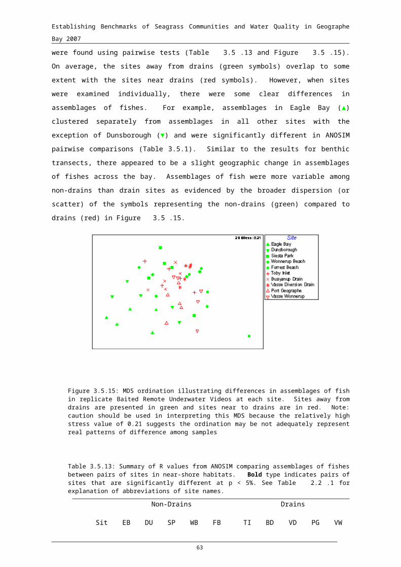
Establishing Benchmarks of Seagrass Communities and Water Quality in Geographe Bay 2007
Table 4.2.17: Summary of Resource Condition Targets (RCTs) and Management Targets (MTs) for NHT and NAP projects and how these have been addressed by Project CM.01b. See Section 1.1 for full details of RCTs and MTs.
Principle RCTs or MTs How project has met, or is meeting RCTs and MTs
MRCT1Marine habitat integrity improved by 2025
Data collected will aid identification of impacts. Amelioration of impacts (e.g. nutrient reduction in the catchment as part of Coastal Catchment Initiative) will then improve integrity of seagrass habitats.
MT1Gaps in marine knowledge identified
Baseline data will fill a knowledge gap in seagrass ecosystem and water quality processes in Geographe Bay and provide basis for long term management.
MT4Critical marine ecosystem processes
Links between nutrient data, light data and seagrass characteristics are being evaluated to assess processes that affect Geographe Bay seagrass communities.
MT5 Baseline informationData collected will serve as a baseline against which future changes may be measured and detected.
MT9 Long term monitoring program
The sites, methods and project design form a monitoring program that can be implemented for the long term assessment of the health of seagrass communities in Geographe Bay. This data may also provide a basis to detect changes in seagrass communities due to climate change, marine pests and coastal urbanisation.
MT10
Conservation status of at-risk species. Monitoring of biodiversity assets, population trends, regionally significant species
The status of species that are at risk of impacts, at the sampling locations, (i.e. seagrasses or their associated biota) are being identified. Biodiversity and population trends of assemblages are being quantified (i.e. seagrasses, fishes, invertebrates). New species and species beyond their known range are being identified including sponge species’ that are likely new to science.
MT21 Community awareness increasedPresentations have been given to Government Departments and non-government organisations. Media coverage has also been gained in newspapers, electronic bulletins and magazines.
WRCT16
Reduce water related point source and diffuse pollution. Standard water quality dataset and health inventory
Water quality data have been collected at all sites and link with monitoring by the Department of Water and the Coastal Catchments Initiative.
SUMMARY - DISCUSSION
Patterns of seagrass growth at Toby Inlet, Siesta Park and Port Geographe suggest these sites warrant
more intensive investigation
Large variability among sites suggests that the detection of impacts at specific drains will require more
intensive sampling effort with the addition of multiple sites
Rocky reefs are likely to be influencing assemblages of fishes, invertebrates and epiphytes
High number of fish species identified (76) compared to previous scientific studies of Geographe Bay
Absence of patterns in epiphyte growth on ASUs was not unexpected because sampling was in
Autumn when nutrient loads are considered low
Diversity of invertebrates appears high compared to other temperate seagrass meadows
Preliminary data suggest water quality was generally good in March 2007
Project is meeting a range of RCTs and MTs as outlined by SWCC in the South West Regional
Strategy for Natural Resource Management
63

Establishing Benchmarks of Seagrass Communities and Water Quality in Geographe Bay 2007
5 REFERENCES
Anderson, M.J., 2001. Permutation tests for univariate or multivariate analysis of variance and regression. Canadian Journal of Fisheries and Aquatic Sciences 58, 626-639.
Anderson, M.J., 2005. PERMANOVA - Permutational multivariate analysis of variance. Department of Statistics, University of Auckland, Auckland.
Anderson, M.J., Gorley, R.N., 2007. PERMANOVA+ for PRIMER: Guide to Software and Statistical Methods. PRIMER-E, Plymouth, UK.
ANZECC, 2000. Australian guidelines for water quality monitoring and reporting. Australian and New Zealand Environment and Conservation Council / Agriculture and Resource Management of Australia and New Zealand, Canberra, pp. 47.
Ayvazian, S.G., Hyndes, G.A., 1995. Surf-zone fish assemblages in South-Western Australia - Do adjacent nearshore habitats and the warm Leeuwin Current influence the characteristics of the fish fauna. Marine Biology 122, 527-536.
Barnes, P.B., Davis, A.R., Roberts, D.E., 2006. Sampling patchily distributed taxa: a case study using cost-benefit analyses for sponges and ascidians in coastal lakes of New South Wales, Australia. Marine Ecology-Progress Series 319, 55-64.
Cambridge, M.L., Kendrick, G.A., 2000. Habitat Mapping: Environmental Studies for Proposed Ocean Outlet, Bunbury Waste Water Treatment Plant. . The University of Western Australia & Alex Wyllie and Associates, Perth.
Cambridge, M.L., Chiffings, A.W., Brittan, C., Moore, L., McComb, A.J., 1986. The loss of seagrass in Cockburn Sound, Western Australia II. Possible cause of seagrass decline. Aquat. Bot. 24, 269-285.
Cappo, M., Harvey, E., Malcolm, H., Speare, P., 2003. Advantages and applications of novel “video-fishing” techniques to design and monitor Marine Protected Areas. In: Beumer, J.P., Grant, A., Smith, D.C. (Eds.), “Aquatic Protected Areas - What works best and how do we know?", Proceedings of the World Congress on Aquatic Protected Areas, Cairns, Australia, pp. 455-464.
Chittaro, P.M., 2004. Fish-habitat associations across multiple spatial scales. Coral Reefs 23, 235-244.Clarke, K.R., 1993. Non-parametric multivariate analyses of changes in community structure. Aust. J. Ecol.
18, 117-143.Clarke, K.R., Warwick, R.M., 2001. Changes in marine communities: An approach to statistical analysis and
interpretation. Plymouth Marine Laboratory, UK.Coleman, N., 2007. Sea stars and echinoderms of the Asia/Indo-Pacific. Neville Coleman's Underwater
Geographic Pty Ltd, Springwood, Australia.DEP (WA), 1996. Southern metropolitan coastal waters study. Final report. Department of Environmental
Protection (Marine Impacts Branch), Perth.Farnsworth, E.J., Ellison, A.M., 1996. Scale-dependent spatial and temporal variability in biogeography of
mangrove root epibiont communities. Ecological Monographs 66, 45-66.Friedlander, A.M., Parrish, J.D., 1998. Habitat characteristics affecting fish assemblages on a Hawaiian coral
reef. Journal of Experimental Marine Biology and Ecology 224, 1-30.Glasby, T.M., Underwood, A.J., 1996. Sampling to differentiate between pulse and press perturbations.
Environmental Monitoring and Assessment 42, 241-252.Harlin, M.M., 1973. Obligate algal epiphyte: Smithora naiadum grows on a synthetic substrate. J. Phycol. 9,
230-232.Horner, S.M.J., 1987. Similarity of epiphyte biomass distribution on Posidonia and artificial seagrass leaves.
Aquatic Botany 27, 159-167.Howard, R.K., 1989. The structure of a nearshore fish community of Western Australia: Diel patterns and the
habitat role of limestone reefs. Env. Biol. Fish. 24, 93-104.Hyndes, G.A., E., P.M., C., P.I., C., L.R., 1999. Does the composition of the demersal fish assemblages in
temperate coastal waters change with depth and undergo consistent seasonal changes? Marine Biology 134, 335-352.
Kendrick, G.A., Aylward, M.J., Hegge, B.J., Cambridge, M.L., Hillman, K., Wyllie, A., Lord, D.A., 2002. Changes in seagrass coverage in Cockburn Sound, Western Australia between 1967 and 1999. Aquat. Bot. 73, 75-87.
Lord and Associates, 1995. Geographe Bay Study 1993-1995 Summary Report. D.A. Lord and Associates in association with Centre for Water Research, University of Western Australia and Department of Botany, University of Western Australia for Water Authority of Western Australia (Southwest Region), Perth.
Marba, N., Walker, D.I., 1999. Growth, flowering, and population dynamics of temperate Western Australian seagrasses. Marine Ecology Progress Series 184, 105-118.
McMahon, K., I., W.D., 1998. Fate of seasonal, terrestrial nutrient inputs to a shallow seagrass dominated embayment. Estuar. Coast. Shelf Sci. 46, 15-25.
64

Establishing Benchmarks of Seagrass Communities and Water Quality in Geographe Bay 2007
McMahon, K., Young, E., Montgomery, S., Cosgrove, J., Wilshaw, J., Walker, D.I., 1997. Status of a shallow seagrass system, Geographe Bay, southwestern Australia. J. Royal Soc. W.A. 80, 255-262.
Neverauskus, V.P., 1987. Accumulation of periphyton biomass on artificial substrates deployed near a sewage sludge outfall in South Australia. Estuarine, Coastal and Shelf Science 25, 509-517.
Platell, M.E., Potter, I.C., 2001. Partitioning of food resources amongst 18 abundant benthic carnivorous fish species in marine waters on the lower west coast of Australia. Journal of Experimental Marine Biology and Ecology 261, 31-54.
PRIMER-E Ltd, 2005. Plymouth routines in multivariate ecological research. PRIMER 6 for Windows version 6.1.2, Plymouth, UK.
Scott, J.K., 1981. The seagrass fish fauna of Geographe Bay, Western Australia. Journal of the Royal Society of Western Australia 63, 97-102.
Searle, J.D., 1977. Sedimentation in Geographe Bay, Western Australia, Department of Geology. University of Western Australia, Crawley.
Silberstein, K., Chiffings, A.W., McComb, A.J., 1986. The loss of seagrass in Cockburn Sound, Western Australia III. The effect of epiphytes on productivity of Posidonia australis Hook f. Aquatic Botany 24, 355-371.
SKM, 2003. Integrated nearshore marine monitoring program for southern Geographe Bay. Sinclair Knight Merz, Coasts and Clean Seas, Water Corporation, Natural Heritage Trust., Perth.
Southwest Development Commission, 2004. Population growth projections for the Southwest of Western Australia. .
SWCC, 2005. South West Regional Strategy for Natural Resource Management. South West Catchments Council, Bunbury, pp. 178.
Underwood, A.J., 1981. Techniques in analysis of variance in experimental marine biology and ecology. Oceanography and Marine Biology an Annual Review 19, 513-605.
Underwood, A.J., 1992. Beyond BACI: The detection of environmental impacts on populations in the real, but variable, world. Journal of Experimental Marine Biology and Ecology 161, 145-178.
Underwood, A.J., 1994. On beyond BACI: Sampling designs that might reliably detect environmental disturbances. Ecological Applications 4, 3-15.
Van Elven, B.R., Lavery, P.S., Kendrick, G.A., 2004. Reefs as contributors to diversity of epiphytic macroalgae assemblages in seagrass meadows. Marine Ecology-Progress Series 276, 71-83.
Wernberg, T., Vanderklift, M.A., How, J., Lavery, P.S., 2006. Export of detached macroalgae from reefs to adjacent seagrass beds. Oecologia 147, 692-701.
White, K., Roux, J., Walker, D.I., 2006. Recommendations for future monitoring of the seagrass ecosystem in Geographe Bay. Funded by the National Action Plan for Salinity and Water Quality, pp. 26.
Willis, T.J., Babcock, R.C., 2000. A baited underwater video system for the determination of relative density of carnivorous reef fish. Marine and Freshwater Research 51, 755-763.
Winer, B.J., Brown, D.R., Michels, K.M., 1991. Statistical Principles in Experimental Design. McGraw-Hill, New York.
65

Establishing Benchmarks of Seagrass Communities and Water Quality in Geographe Bay 2007
6 APPENDIX - DATA TABLE
Table 4.2.18: Mean abundance (Max N) of fish species recorded in baited remote underwater video (BRUV) at each site (see Table 2.2.1 for site codes). Some identifications are to be finalised and are marked unknown or presented as the genus followed by sp.
66