
Belt driven Alternator and Starter with a Series … driven Alternator and Starter with a Series...
115
Belt driven Alternator and Starter with a Series Magnetized Synchronous Machine drive Tomas Bergh Licentiate Thesis Department of Industrial Electrical Engineering and Automation 2006
Transcript of Belt driven Alternator and Starter with a Series … driven Alternator and Starter with a Series...

Belt driven Alternator and Starter with a Series
Magnetized Synchronous Machine drive
Tomas Bergh
Licentiate Thesis Department of Industrial Electrical Engineering and Automation
2006

ii
Department of Industrial Electrical Engineering and Automation Faculty of Engineering Lund University Box 118 221 00 LUND SWEDEN http://www.iea.lth.se ISBN 91-88934-44-6 CODEN:LUTEDX/(TEIE-1052)/1-115/(2006) © 2006 Tomas Bergh Printed in Sweden by Media-Tryck, Lund University Lund 2006

iii


v
Abstract
Electric Hybrid Vehicles, EHV, are under development to provide lower fuel consumption levels and minimize the environmental pollution compared to pure Internal Combustion Engine, ICE, driven vehicles. The EHV is more complex and thus carry many more extra parts than the pure ICE based vehicle. Competing against the pure ICE vehicle in the sense of non-expensive mass production is hard.
This thesis is a result of a research project with the goal to develop a complete Belt driven Alternator and Starter, BAS, system for a Stop&Go functionality as a cost-effective hybrid vehicle solution. BAS is based on a Series Magnetized Synchronous Machine, SMSM, which as an adjustable-speed drive system comprises power electronics but excludes permanent magnets.
BAS is a rather old concept. It merges two functions, an electric starting motor and an generator, into one single electric machine. It thereby makes the total system lighter and smaller. Furthermore, it facilitates technology leaps on the road towards mass production of electric hybrid vehicles.
The developed BAS system is suitable for a midrange passenger vehicle. The Stop&Go functionality provides an ICE turn-off at each vehicle stop. The SMSM is, in addition to generating electricity and starting the ICE, intended to support the ICE with an additional torque when it is assumed beneficial in the sense of reaching low fuel consumption.
Topics in the field of power electronics and control of the SMSM that are covered in this thesis are:
• Simulations on vehicle basis are performed for optimizing the rated power of the electric machine and its power electronics in the sense of low fuel consumption.
• The Series Magnetized Synchronous Machine, SMSM, and the theory lying behind it are presented. The SMSM is carefully investigated both magnetically and electrically.

• A simulation model for the SMSM is derived based on the theoretical model that describes the SMSM.
• Based on the theoretical model of the SMSM, dedicated current controllers are derived. Other types, as standard PI controllers and a so-called field voltage vector feed forward controller are investigated and simulated for control of the SMSM.
• The SMSM is tested in laboratory environment for confirming the behaviour of the derived model of the adjustable-speed drive system including its power electronics.

vii
Acknowledgements
First, I would like to thank my friend and colleague Dan Hagstedt for these two and a half years of cultivating cooperation. Dan has filled the very important and sometime burdensome role as discussion partner and he gave encouragement those days it was of importance.
I have had the honour to be working together with Professor Mats Alaküla, my main supervisor. Mats has, besides his very deep and wide knowledge, the ability to encourage and inject engagement.
Dr. Per Karlsson has acted as assistant supervisor with great skill and he has taught me much. Per has a special interest in power electronics, a topic that I find very interesting myself. Per has developed, from being a secondary supervisor, to a person that I look up to and appreciate as a friend. I hope our roads will cross again.
The reference group of this project has provided guidelines, critics, ideas and knowledge at the arranged reference group meetings. The group included Rolf Ottersten (GME Engineering), Lars Hoffman (GME Engineering), Ola Carlsson (Chalmers University), Göran Johansson (Vtec) and Sture Eriksson (Royal Institute of Technology) as well as my two supervisors and Dan Hagstedt.
This project is funded by the Swedish Government and the automobile manufacturer SAAB. I am glad for being given the opportunity to participate and develop in this project.
Lars Gertmar at ABB has helped with his valuable experience, comments and discussions.

viii
Family and people in my professional and personal surroundings have contributed in several different important ways from friendship and laughs to assisting in the lab. Different universities offered interesting courses to participate in and people to share fruitful discussions with. Although not mentioned by name, I hope you all know your own valuable contribution.
The two companies Future Electronics and Beving Elektronik sponsored with components.
Thank you all!
Lund, 23 October 2006
Tomas Bergh

ix
Contents
CHAPTER 1 INTRODUCTION............................................................11 1.1 RESEARCH OBJECTIVES .............................................................11 1.2 PREVIOUS WORK........................................................................12 1.3 AUTHOR’S OPINION, DRIVING FORCE AND REFLECTIONS ..........13 1.4 OUTLINE OF THE THESIS............................................................17
CHAPTER 2 POWER ELECTRONICS IN A BAS APPLICATION19 CHAPTER 3 ELECTRIC MACHINE TOPOLOGIES ......................21
3.1 THE INDUCTION MACHINE, IM ..................................................21 3.2 THE SYNCHRONOUS MACHINE, SM ..........................................22
The Permanently Magnetized Synchronous Machine, PMSM ..........23 The Electrically Magnetized Synchronous Machine, EMSM ............24 The Series Magnetized Synchronous Machine, SMSM......................24
3.3 THE DIRECT CURRENT MACHINE, DC ......................................25 The Permanently Magnetized Direct Current Machine, PMDC .......25 The Electrically Magnetized Direct Current Machine, EMDC.........26 The Series Magnetized Direct Current Machine, SMDC ..................27 The Parallel (Shunt) Magnetized Direct Current Machine...............27 The Compound connected Direct Current Machine..........................27 The Brushless Direct Current Machine, BLDC.................................27
3.4 THE SWITCHED RELUCTANCE MACHINE, SRM ........................28 CHAPTER 4 PREPARATORY RESEARCH, SIMULATIONS ON VEHICLE BASIS ....................................................................................29 CHAPTER 5 MODELLING THE SMSM............................................35 CHAPTER 6 DEVELOPMENT OF A SIMULATION MODEL OF THE SMSM..............................................................................................47 CHAPTER 7 CONTROL METHODS..................................................55

x
7.1 DEDICATED VECTOR BASED CURRENT CONTROLLER ............... 55 7.2 FIELD VOLTAGE VECTOR FEED FORWARD................................. 60 7.3 TORQUE COMPENSATION .......................................................... 61
CHAPTER 8 SIMULATION RESULTS.............................................. 65 8.1 IMPLEMENTATION OF SIMULATION MODEL............................... 65 8.2 SMSM CONTROLLED BY STANDARD SM PI CONTROLLERS..... 71 8.3 SMSM CONTROLLED BY DEDICATED CONTROLLER................. 76 8.4 SMSM CONTROLLED BY FIELD VOLTAGE VECTOR FEED FORWARD .............................................................................................. 81 8.5 TORQUE COMPENSATION .......................................................... 85
CHAPTER 9 LABORATORY RESULTS ........................................... 89 9.1 LABORATORY EQUIPMENT ........................................................ 89 9.2 MEASUREMENTS ....................................................................... 90
Standard PI control of SMSM........................................................... 91 CHAPTER 10 DEVIATIONS BETWEEN SIMULATION AND LABORATORY RESULTS................................................................... 99
10.1 CONSEQUENCES OF THE DEVIATIONS...................................... 104 CHAPTER 11 CONCLUSIONS.......................................................... 105 CHAPTER 12 FUTURE WORK ........................................................ 109 BIBLIOGRAPHY................................................................................. 111

11
Chapter 1 Introduction
1.1 Research objectives
The objectives of this thesis are to develop parts of an assistive electric drive for a midrange passenger vehicle based on a Series Magnetized Synchronous Machine (SMSM). The electric drive shall be able to apply Stop&Go functionality and to add an additional torque at lower speeds were the Internal Combustion Engine (ICE) does not perform very well in terms of efficiency or torque production. The electric drive shall be able to cooperate with a 1.9 litre diesel ICE. The Stop&Go functionality provides an ICE turn-off at each vehicle stop and thus minimizes unnecessary exhausts that in fact contribute to a large extent of the emissions in urban traffic driving. When the driver initiates acceleration, the electric drive immediately starts the ICE and then produces an accelerating torque to support the ICE. The description of this hybrid vehicle fits well into the Mild Hybrid Electric Vehicle, MHEV, category. For being able to determine a more accurate comparable level of hybridization, the Electric Hybridization Rate, EHR Jonasson K. (2002), can be calculated. The EHR corresponds to the quotient between the electric traction power and the total traction power. The EHR level is calculated after the size of the electric machine is determined in Chapter 4.
The Belt driven Alternator and Starter, BAS, system is intended to be a simple and easy to install system that is compatible with vehicles already on the market. The vehicle manufacturer avoids making any large reconfigurations of a standard vehicle when installing the BAS system.

12 Chapter 1. Introduction
1.2 Previous work
In recent years much effort has been put into research related to hybrid vehicle development, both at universities and in the private sector. There are already many commercial HEVs available on the market today. The Citroén C3 is an example of a vehicle with Stop&Go functionality but no hybridization feature.
In the beginning of the project resulting in this thesis, there was a discussion of which voltage level that is most suitable for this Mild Hybrid Electric Vehicle, MHEV. The first idea was to use 42V, which is a voltage level that also can be suitable for introduction into the standard personal vehicles without any hybridization feature. Much research is done investigating different power electronic converter topologies operating at a voltage level of 42 V in passenger vehicles i.e. Jourdan L. (2002). The on-board loads in personal vehicles tend to increase and therefore require higher currents, Marksell S. (2004). For avoiding high currents that require coarse and clumsy conductors, there is a discussion about changing from today’s systems 14V to 42V. This discussion has been ongoing for some time but no car manufacturer seems to be willing to take the first expensive step. On the other hand, when there is more on-board electric power available, the electric loads tend to increase even more leading to that the currents will be high anyway. This discussion continues and voices argue that if we are going to introduce a higher standard voltage level in personal vehicles, why not increase it up to 200 or 300V that is suitable also for standard HEV? If the voltage level is increased to a few hundred volts, several other issues arise such as safety issues and electric insulation.
Much effort is put into developing belt-driven MHEV systems for 42V around the world. The type of electric machine that is used as a generator in vehicles of today is called Lundell generator. The Lundell generator is a claw-pole electrically excited synchronous machine that in vehicle application suffers from a rather low efficiency that is between 50 and 60%. The Lundell generator is robust, inexpensive, simple to produce and control and has a wide range of operation.
Publications are available, showing that people are working much in this field for developing a generator with a higher efficiency than the Lundell generator and with good robustness, simplicity, low cost in production and wide range of operation. Examples of references relating to this topic are Reiter F.B.

1.3. Author’s opinion, driving force and reflections 13
(2001), Shaotang C. (2001), Nicastri P.R (2000), Mudannayake C.P. (2003).
1.3 Author’s opinion, driving force and reflections
In a wide perspective, projects like that behind this thesis are efforts for achieving lower fuel consumption and thereby better chances for a sustainable development. Since environmental issues are very close to my heart, this area does not attract me only due to my technical interest.
During the work I have realized that many projects of this kind mostly are driven by the fear of future depletion of energy resources. In most cases this results in the question; “How shall we produce the energy required by the consumers?”. Since energy waste, in my opinion, is the superior problem of today, securing energy resources is not the right focus. All energy that is exploited today, except the energy derived from wind-, water-, or sun-powered plants, produces some kind of pollution. The energy produced by the clean power plants that are installed today, is unfortunately only enough for supplying a few percent out of what is consumed. Thus, in order to achieve less pollution the energy consumption aught to be minimized.
Many research projects are often based on enhancements of older techniques (in this case the Otto engine). These projects mainly deliver solutions that lower the energy consumption by a mere few percents. Taking into account these small reductions of energy consumption and the estimated increment of the transport fleet over the next 24 years, European Commission (2003), the energy exploitation will still be increasing.
According to the report from the European Commission (2003), there were 468 private cars per 1000 habitants at the year of 2003 in the European Union. The private vehicle fleet is expected to increase with 1.2% per year until year 2030, which denotes a total increment of 33%. This gives 623 personal cars per 1000 habitants. The importance of preventing this development is clearly stated in the report mentioned above;
“The transport sector is one of the most important sectors from the viewpoint of both energy consumption and environmental implications. The near complete dependence of the sector of oil products generates two sorts of concern: security of oil supplies with rising needs for transportation purposes; and worries about climate change...”

14 Chapter 1. Introduction
Development producing more energy efficient solutions is important for minimizing the energy consumption but an even more valuable tool for changing the trend with increasing energy usage is by influencing the human behaviour.
Unfortunately, people tend to make decisions that are irrational and non-optimized in the long run. Decision-making parameters such as individual comfort and status do in most cases override parameters that ensure sustainable development for the individual as well as for every other living being.
Due to this irrational behavior there is a need for methods and tools to influence human behavior. The most obvious method might be to increase people’s awareness of how their behavior affects the environment.
First, I believe it is important to understand how much energy a common citizen (Swedish) use. For achieving this, a good reference can be how much power a person is able to produce by hand. According to Bengtsson H.U. (1998), an average person is able to develop a peak power of approximately 300W and it is recommended not to exceed 40% out of that maximum power when performing work that lasts for longer times. Let us then assume that one person is able to produce a power of approximately 100W continuously.
As a comparison, I will try to calculate the amount of energy used per person when travelling from Stockholm in Sweden to Sydney in Australia. The type of aeroplane that is used for such long trips is e.g. the Airbus 340. This plane consumes approximately 8800l fuel (of type Jet A-1) per hour and from Stockholm to Sydney there is also an intermediate landing in Bangkok. The total travelling time is approximately 19 hours that gives a total fuel consumption of 167200l for 245 persons according to the airline company SAS. The distance (8270km + 7530km) together with mentioned information gives a fuel consumption of 0.43 l /person and 10km of flight fuel. This is a number that is in the same order as the fuel consumption of a standard personal vehicle of today.
Of course, the flight fuel has approximately 7% higher energy density per litre than ordinary petrol (that has an energy density of 32MJ/l) so the equivalent fuel consumption is 0.46l/km. Anyway, the total amount of consumed fuel is 682.4l/person and trip that give 23367MJ/person and trip

1.3. Author’s opinion, driving force and reflections 15
(with an energy density of 34.2MJ/l and a density of 800kg/m3) this equals approximately 6490 kWh/person and trip.
For a family with four members, a two-way ticket gives an energy usage of approximately 52000 kWh. A typical household in Sweden consumes about 25000 kWh annually, including heat- and electricity. Therefore, the trip to Australia costs, in terms of energy, as much energy as the supply for a typical household during two years.
For earning the energy that is consumed using a two-way ticket between Stockholm in Sweden and Sydney in Australia, a normal person has to work in 129800100/12980000 =WWh hours or 14.8 years, night and day.
Applying the same logic on everyday transportation gives another comparison. An average Swedish person (in the age between 6 and 65 years) travels 30 km/day to and from his work or school (Statistics Sweden, www.scb.se). Assuming that an average person travels by car, that consumes 0.75l/10km, to and from his work gives an energy usage that corresponds to 200 hours of physical work each day.1
In Figure 1.1 we can see the development of the energy usage in Sweden from 1970 to 2004. There is a clear increasing trend, shown by the solid line in the figure that indicates an annual increment of the energy usage of 5.9TWh.
1 To be compared with 1.5 hours of physical work if travelling by bicycle.

16 Chapter 1. Introduction
1970 1975 1980 1985 1990 1995 20000
100
200
300
400
500
600
700
800
Year
Ener
gy [T
Wh]
Non-energy purposes, bunkers etc.Internal transportIndustryResidential, services etc.
Figure 1.1. Energy usage in Sweden from 1970 to 2004. Information from the Swedish Energy Agency.
Lars Hoffman in the reference group of this project once told me something that really etched itself into my memory. Many persons think it is not a fair comparison but I think it is very good and puts the energy usage in a relation to, also in this case, physical work. The comparison is also highly interesting with regards to the almost constantly rising price of petrol. Lars said something similar to: “I think the petrol for my car is really cheap!” and of course, no one understands this statement from the beginning. How much do you want to be paid for pushing my car one kilometre? Guessing that it will take approximately 20 minutes2 on a flat road and quite a big physical effort is a sign good enough for expecting that your answer is at least 100SEK. A modern standard personal car of today consumes between 0.5 and 1.0l petrol per 10km that costs approximately 11.5SEK/l today, gives a fuel cost per 2 The guessed transporting time of 20 minutes can also be estimated by calculation. The fuel consumption is approximately 0.06l/km that equals 1.92MJ of energy. Guessing the average efficiency of the engine, driveline and frictions to 10% means that 0.192MJ is actually transferred from chemical energy to transporting energy. 0.192MJ equals 53Wh that takes approximately half an hour to produce by hand for an intermediate person.

1.4. Outline of the Thesis 17
kilometre of approximately 86.010/5.1175.0 ≈⋅ SEK/km. Thus the price of the performed work, using petrol, is less than 1% compared to if it is carried out by hand. Still we are complaining of how expensive the petrol is!
Besides increasing people’s awareness of what effects their behaviour has on the environment, I believe other behaviour enforcing measures of action might be necessary as well.
One way might be to increase taxes on different energy types radically at carefully selected points. Of course there must be a carefulness that sets the increment on the right spots as we do not want the industry to move from Sweden or that people begin to heat their houses using oil instead of using available environmentally better methods. The development of energy efficient systems would most certainly explode.
Another radical method can be to introduce rations of energy, similar to the current system with tradable pollution rights. If a person drives a very large car, there will be less energy left for heating up his house. Alternatively, if a person has a very large house that needs to be heated up, there will be little energy left for car driving.
A less forceful method, perhaps complementary, to induce behaviour change might be to increase the status of goods that are compatible with sustainable development. This increased status has already occurred on the Hybrid Electric Vehicle (HEV) market. Many of those who buy the first, mass produced HEV on the market, the Toyota Prius, probably does not only buy it for the environmental goodwill reason and the economical in terms of lower fuel consumption, but also because it gives a push on their status. Unfortunately the decision should be, in my opinion, to travel less instead of buying another car. But as we can see, using marketing forces to make aware decisions trendy may be applicable to many different fields for influencing the consumers in a positive way.
As a conclusion, there is a need for technical development but more important; there is a great need for a change in human behaviour.
1.4 Outline of the Thesis
In this section, the outline of the thesis is presented. The thesis consists of 12 chapters that are briefly described below.

18 Chapter 1. Introduction
Chapter 1 that is the introduction provides the objectives, previous work, the author’s personal opinion and reflections and this outline.
Chapter 2 discusses Power Electronics in brief relating it to this specific application.
For readers that are not very familiar with electric machines, chapter 3 gives a very shallow physically and magnetically related description of different types of electric machines to compare with the Series Magnetized Synchronous Machine, SMSM.
The Stop&Go functionality is implemented in available hybrid vehicle simulation models with a summary of the simulation results on vehicle basis briefly presented in chapter 4.
In chapter 5, a mathematical electromagnetic model of the SMSM is derived.
In chapter 6, the SMSM model, derived in previous chapter is extended to a simulation model.
Different controller types are investigated in chapter 7. First, a dedicated controller for the SMSM is derived. Secondly, an approach called “Field voltage vector feed forward” is described and finally a method for forcing the SMSM to produce a constant torque is presented.
Results from simulations controlling the SMSM and utilizing the different controllers presented in the previous chapter are presented in chapter 8.
Measurement results from operating a SMSM in the laboratory in chapter 9. Measurements are performed for determining the validity of the derived SMSM model.
In chapter 10 there is a discussion of the differences between simulation results and measurement results.
In chapter 11, some conclusions are drawn followed by chapter 12 where topics that can be interesting to follow up are presented.
A short list of abbreviations in the topic is available in Appendix A.

19
Chapter 2 Power Electronics in a BAS application
A definition of Power Electronics is stated in Wilson T. G. (2000) as;
Power electronics is the technology associated with the efficient conversion, control and conditioning of electric power by static means from its available input form into the desired electrical output form.
In the same transaction as above, the goals of using Power Electronics are also stated;
The goal of power electronics is to control the flow of energy from an electrical source to an electrical load with high efficiency, high availability, high reliability, small size, light weight, and low cost.
For the BAS application, all of the mentioned goals are necessary to be fulfilled.
The automotive market introduces high demands on the power electronics manufacturers concerning reliability and temperature requirements. The power electronic equipment is in this case meant to be placed in the engine compartment where the temperature is expected to vary between –40°C and +150°C. Semiconductors of different technologies are suitable for different types of applications. Voltages below approximately 200V and high temperature applications are recommended to apply the MOSFET technology, Campbell R.J. (2004).
The semiconductor manufacturers are striving to increase the maximum allowed operating temperatures, which is good for the automotive sector that, as mentioned, has very high temperature demands. The power electronic

20 Chapter 1. Introduction
semiconductors’ performances have increased much during the last decade. The MOSFET technology is able to handle almost the double current density (current / die area) at the die cost of approximately 60% of compared to 1995.
Even if the maximum allowed die operating temperature has increased much, up to 175°C, it is still a great challenge to design the cooling and inverter for ambient temperatures of +150°C.
There have been discussions about utilizing SiC (Silicon Carbide) semiconductor devices in this project. Research on the SiC transistor technology is, and has been, in progress during several years by now but this technology has not reached its commercial breakthrough yet. The basic features of SiC are promising such as very short switching times, high breakdown voltage levels and it is also able to operate in very high ambient temperatures. But even if the operating temperature of the material SiC can be very high, other issues comes into the light as packaging and bonding. Drawbacks are that the SiC transistors are bipolar and thus current-controlled which means that they require more advanced driver circuits. The SiC are also extremely expensive because of a slow and very high temperature demanding manufacturing process. The SiC transistor technology is in the author’s opinion not ready to be used in a commercial cost-optimized vehicle of today where every cent in the production cost is scrutinized in detail.
The Series Magnetized Synchronous Machine, SMSM, is a three-phase machine with one connector for each phase. The power electronic converter in the BAS application is based on a three-phase MOSFET full-bridge power electronic device. The power electronic converter operates as a DC to AC (three-phase) converter when the electric machine operates as a motor and AC (three-phase) to DC converter when the electric machine operates in generator mode.

Chapter 3 Electric machine topologies
In this chapter, the principles of different rotating electric machine types are described briefly.
3.1 The induction machine, IM
The induction machine that also is called the asynchronous machine is the most widely used electric machine type. The asynchronous machine has several advantages such as robustness and non-complicated design and use. It has a very robust mechanical design and is cost effective in production. The asynchronous machine requires more power electronics and a more complex control than e.g. the DC machine. An induction machine with special design for reaching high torque density, power density and efficiency is a strong competitor to the synchronous machine topology for the HEV category, Shafer G.A (1994).
The name induction refers to the principle of the machine operation. When the induction machine is connected to the grid, or any suitable AC voltage source, there is a rotating flux generated in the stator. If there is a difference in rotating speed between the stator and the rotor the rotating flux vector induces a voltage in the rotor winding. The difference between the rotating speed and the rotating speed of the flux is called the slip speed. The induced voltage results in a rotor current that generates a flux in the counter direction to the flux generated by the stator windings.
The other name, asynchronous machine, refers to that there is a difference between the rotating flux vector speed in the stator and the rotor mechanical speed, thus asynchronous rotation. If there is no speed difference, no voltage is induced, i.e. no current is produced, in the rotor and hence no torque is generated.
22 Chapter 3. Electric machine topologies
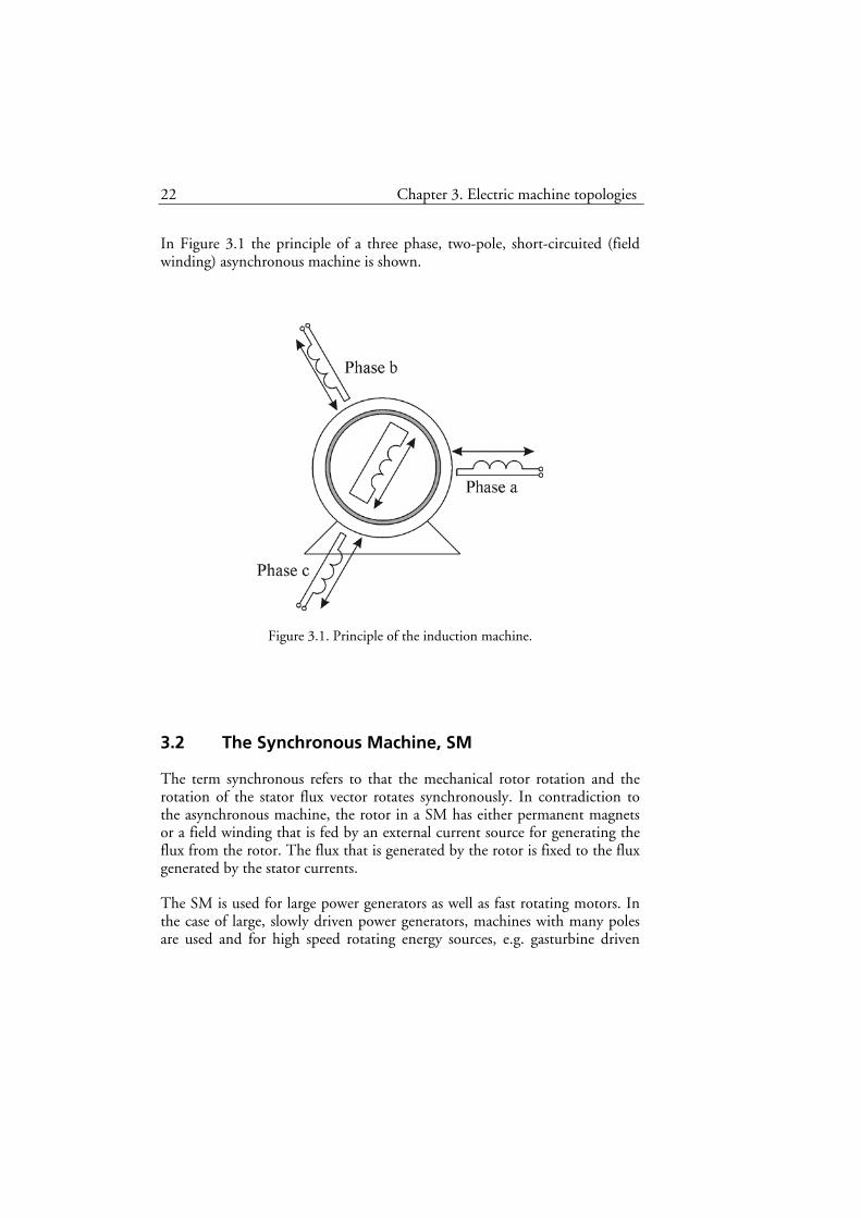
In Figure 3.1 the principle of a three phase, two-pole, short-circuited (field winding) asynchronous machine is shown.
Figure 3.1. Principle of the induction machine.
3.2 The Synchronous Machine, SM
The term synchronous refers to that the mechanical rotor rotation and the rotation of the stator flux vector rotates synchronously. In contradiction to the asynchronous machine, the rotor in a SM has either permanent magnets or a field winding that is fed by an external current source for generating the flux from the rotor. The flux that is generated by the rotor is fixed to the flux generated by the stator currents.
The SM is used for large power generators as well as fast rotating motors. In the case of large, slowly driven power generators, machines with many poles are used and for high speed rotating energy sources, e.g. gasturbine driven

3.2. The Synchronous Machine, SM 23
generators, a machine with low number of poles is used, so called turbo-machines. Synchronous machines in general are known for their high torque and power density and their high efficiency.
The Permanently Magnetized Synchronous Machine, PMSM The PMSM has a rotor equipped with permanent magnets that produce a flux vector fixed to the rotor. PMSMs can have very high torque- and power density capabilities. The rotormagnets can be either surface- or deep mounted. Commonly used high performance magnetic materials are Samarium-Cobolt and Neodynium-Boron-Iron. These types of magnetic materials are resistant to both vibrations and high temperatures. For extending the operating region of the PMSM it is possible to apply field weakening by generating a flux in the opposite direction as generated by the permanent magnets. In this way, the induced voltage in the stator will decrease and it will be possible to operate the machine at higher rotational speed using a limited DC voltage source. Unfortunately, there is a limit for how much negative flux the magnets can withstand before they are demagnetized. This is thus a limit for the operating region flexibility of the PMSM. Loosing the control of a deeply field-weakened PMSM can results in a very high phase voltages that may damage the power electronics and control electronics. The principle of a PMSM is shown in Figure 3.2.
Figure 3.2. Principle of the Permanently Magnetized Synchronous Machine.

24 Chapter 3. Electric machine topologies
The Electrically Magnetized Synchronous Machine, EMSM An EMSM is very similar to the PMSM but differs as it has a rotor equipped with a winding instead of permanent magnets. The rotor winding is mostly fed via slip rings and is generally excited by an external power electronic circuit that controls the field winding current. In this way the field winding current, and hence the flux, can be lowered for reaching higher rotational speeds (field-weakening). Another way of exciting the rotating field winding is to feed it directly from a diode rectifier if the grid is available for the application. However this gives no opportunity to apply field weakening. The operating region of the EMSM is wider than for the PMSM since it is possible to apply very deep field weakening. The principle of an EMSM is shown in Figure 3.3. The EMSM is very attractive for the EHV market thanks to the wide operating region, its high efficiency and torque density.
Figure 3.3. Principle of the Electrically Magnetized Synchronous Machine.
The Series Magnetized Synchronous Machine, SMSM The Series Magnetized Synchronous Machine is in fact a modified EMSM that uses the phase currents for exciting the field winding circuit. In a SMSM, the open end of a Y-connected EMSM is fed into a three-phase diode bridge rectifier. The rectifier then supplies energy to the field winding via slip rings. Hence, the field winding current is strictly dependent on the synchronous machine phase currents and the conduction state of the diode bridge rectifier.

3.3. The Direct Current Machine, DC 25
The principle of the SMSM can be seen, similar to the EMSM, on the left of Figure 3.4. To the right of Figure 3.4 the circuit configuration of the SMSM can be seen were the three phase windings, on the left, are connected to the six diodes in the three phase rectifier feeding the field winding on the right. The field winding inductance of a SMSM is lower than the field winding inductance of an EMSM. The SMSM circuit and principle reminds much of the well-known Series Magnetized Direct Current Machine. The SMSM is expected to perform very well in an EHV application thanks to the high torque and power density of synchronous machines.
Figure 3.4. Principle of the Series Magnetized Synchronous Machine (left) and circuit configuration (right).
3.3 The Direct Current Machine, DC
The DC machine is a widely used type of motor available from very low power ratings as milliwatts to very high power ratings as megawatts. One advantage of the DC machine is that it is simple to control and requires less surrounding power electronics than other electric machines. Disadvantages of the DC motor are such as more complicated/expensive to produce and the presence of mechanical commutators with carbon brushes that need maintenance.
The Permanently Magnetized Direct Current Machine, PMDC As Figure 3.5 indicates the field in a PMDC is generated by permanent magnets that are mounted in the stator. The armature winding, the winding

26 Chapter 3. Electric machine topologies
where a voltage is induced, is in the rotor and hence fed via slip rings. As a DC voltage is applied on the armature winding connectors, to the left in Figure 3.5, the current always flows downwards in the figure. The magnetic field, produced by the armature winding, produces a turning torque when interacting with the flux generated by the stator magnets. As the rotor turns a half revolution, the commutators mechanically switch polarity and maintain a current flow direction downwards. The produced torque is still acting in the same rotating direction as before the commutation. The PMDC is an expensive machine that requires maintenance of the brushes and it is not possible to extend the operating region by field-weakening.
Figure 3.5. Principle of the Permanently Magnetized Direct Current machine.
The Electrically Magnetized Direct Current Machine, EMDC The principle of the EMDC is shown in Figure 3.6. The operation is similar to the PMDC but the stator field flux is instead of generated by permanent magnets generated from a field winding.
Figure 3.6. Principle of the Electrically Magnetized Direct Current machine.

3.3. The Direct Current Machine, DC 27
The Series Magnetized Direct Current Machine, SMDC A series magnetized direct current machine is equivalent to the EMDC but with the field winding and armature winding connected in series. The SMDC is also known as the Universal motor that is very widely used.
The Parallel (Shunt) Magnetized Direct Current Machine A parallel magnetized direct current machine is equivalent with the EMDC but with the field winding and armature winding connected in parallel.
The Compound connected Direct Current Machine The Compound connected Direct Current machine is a combination of the Series- and Parallel Magnetized DC machine. The field winding is in this case separated into two windings were one of these is connected in series and the other is connected in parallel to the armature winding. This combination of the field winding gives special torque characteristics.
The Brushless Direct Current Machine, BLDC The BLDC is principally similar to the PMSM differing from that the BLDC has a trapezoidal back EMF, while a PMSM has an approximately sinusoidal back EMF. The back EMF is the voltage that is induced in the stator windings as the flux from the rotor that passes through the stator windings, varies when rotating. No rotation gives no varying flux in the stator, gives no induced voltage that is no back EMF. Outgoing from a DC machine; by moving the field producing permanent magnets from the stator to the rotor and the armature winding to the stator from the rotor, there is no need to transfer energy to the rotor for exciting any winding. Yet, there is a need for a commutator. In the BLDC case the commutations are synchronized with the rotor position and performed electronically by the power electronic devices. The BLDC motor is driven by rectangular voltage strokes that must be carefully applied to two of the three-phase windings. The third phase winding can be used for rotor position estimation. The angle between the stator flux and the rotor flux is kept close to 90° for achieving a maximum torque generation. The BLDC requires intelligent electronics for proper control. The BLDC is a high efficient motor that emits low levels of EMI (compared to DC motors with brushes) but suffers from a higher total system cost than other DC machine drives.

28 Chapter 3. Electric machine topologies
3.4 The Switched Reluctance Machine, SRM
The principle of a SRM (6/4-SRM: Six stator poles and 4 rotor poles) is shown in Figure 3.7. The shown machine is a three-phase machine with two windings per phase. The two windings named equally in the figure are connected in series or in parallel and together form one phase. The generated torque in a SRM is deduced from that the magnetic circuit does wish to minimize the magnetic reluctance in the circuit. The reluctance is a measure of how good a magnetic circuit conduct magnetism. A low reluctance indicates a good magnetic conductivity and vice versa. The reluctance is minimized when the air-gap is as little as possible in the magnetic circuit. At the snapshot in Figure 3.7, phase a produce no torque since the reluctance is already minimized, phase b shall carry a current for generation of a clockwise torque production. The SRM has a simple and robust construction due to the rotor that consists of pure laminated steel and shaft but suffers from bad reputation telling that SRMs produces high noise levels. The noise level is due to the large forces acting in the radial direction that forces the circular rotor to become ellipsoidal. The ellipsoidal shape of the stator rotates with respect to the rotor position.
Figure 3.7. Principle of the Switched Reluctance Machine.

Chapter 4 Preparatory research, simulations on vehicle basis
As a prerequisite, the project behind this thesis was initiated by professor Mats Alaküla together with the automobile company SAAB and partly funded by the government, the application, as mentioned before, focuses on the SMSM in a BAS application.
The simulations on the vehicle basis are performed in the Matlab Simulink environment and based on the earlier derived vehicle model developed by Karin Davidsson (born Jonasson) and Mats Alaküla. The vehicle model is earlier presented in Jonasson K. (2002). Minor modifications in the model are done for adaptation to the Stop&Go functionality. Since this BAS application with Stop&Go functionality mostly implies improvement in terms of lower fuel consumption, in urban driving, simulations are performed using urban driving cycles.
For producing results that are comparable to other researchers’ work simulations are performed using the standardized MVEG-A driving cycle (available on www.dieselnet.com). This cycle is a European driving cycle standard that is accepted as a standard for tests and development concerning emission certification of light duty vehicles in Europe. The MVEG-A driving cycle is based on two other driving cycles that are the ECE 15 and the EUDC (Extra Urban Driving Cycle) driving cycle. First ECE 15 is repeated four times without interruption and is then followed by one EUDC cycle. The four ECE 15 cycles emulates a 4.052km extra urban trip with a maximum speed of 50km/h and an average speed of 18.7km/h (duration of 780s). The EUDC (low powered vehicles) cycle emulates a 6.5km extra urban trip with a maximum speed of 90km/h and an average speed of 60.5km/h (duration of 400s). The MVEG-A driving cycle for low powered vehicles is shown in Figure 4.1.

30 Chapter 5. Preparatory research, simulations on vehicle basis
0 200 400 600 800 1000 12000
10
20
30
40
50
60
70
80
90
100
Time [s]
Spee
d [k
m/h
]
Figure 4.1. The MVEG-A driving cycle.
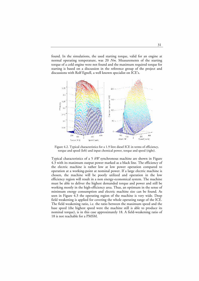
The characteristics of the ICE used in the simulations are shown in Figure 4.2. As there is an electric machine on-board the vehicle it is suitable to let the electric machine assist the ICE at the working-points were the efficiency of the ICE is low and the efficiency of the electric machine is high. Since the idea of the BAS Stop&Go functionality is to deal with the unnecessary fuel consumption during idle operation, the losses for the ICE in idle operation are estimated by calculations. The efficiency map of the 1.9 l diesel engine is recalculated to a map containing the input chemical power that includes the losses introduced in idle operation. This is done for making it possible to determine the gained chemical energy in urban driving cycles. The resulting chemical power consumption map is shown on the right in Figure 4.2. The model for vehicle simulations is modified and is thus instead based on the ICE map containing the input chemical power instead of the ICE efficiency as earlier. The required starting torque is roughly estimated by calculations and introduced as a negative output torque from the ICE at each engine start. The starting torque is very dependent on the temperature of the engine and no solid method for estimating this torque for low temperatures has been
31
found. In the simulations, the used starting torque, valid for an engine at normal operating temperature, was 20 Nm. Measurements of the starting torque of a cold engine were not found and the maximum required torque for starting is based on a discussion in the reference group of the project and discussions with Rolf Egnell, a well known specialist on ICE’s.
Figure 4.2. Typical characteristics for a 1.9 litre diesel ICE in terms of efficiency, torque and speed (left) and input chemical power, torque and speed (right).
Typical characteristics of a 5 kW synchronous machine are shown in Figure 4.3 with its maximum output power marked as a black line. The efficiency of the electric machine is rather low at low power operation compared to operation at a working-point at nominal power. If a large electric machine is chosen, the machine will be poorly utilized and operation in the low efficiency region will result in a non energy-economical system. The machine must be able to deliver the highest demanded torque and power and still be working mostly in the high-efficiency area. Thus, an optimum in the sense of minimum energy consumption and electric machine size can be found. As seen in Figure 4.3 the operating region of the machine is very wide. Deep field weakening is applied for covering the whole operating range of the ICE. The field weakening ratio, i.e. the ratio between the maximum speed and the base speed (the highest speed were the machine still is able to produce its nominal torque), is in this case approximately 18. A field-weakening ratio of 18 is not reachable for a PMSM.

32 Chapter 5. Preparatory research, simulations on vehicle basis
Figure 4.3. Properties of a typical 5 kW electrical machine.
Simulations, utilizing the model for a BAS vehicle and the MVEG-A driving cycle are performed using different electric machine sizes between 2 kW and 100 kW. As we can see in Figure 4.4 there is an optimum of the electric machine size that provides the lowest total energy consumption when driving the MVEG-A driving cycle.

33
0 10 20 30 40 50 60 70 80 90 1000.37
0.375
0.38
0.385
0.39
0.395
0.4
0.405
0.41
Electric machine size [kW]
Fuel
con
sum
ptio
n [L
/100
km]
Figure 4.4. Fuel consumption in relation to electric machine size.
As the electric machine should be physically as small as possible, be able to deliver the required starting torque and provide low fuel consumption, the size of the BAS system that is determined to be developed is 5 kW. The gear factor in the belt transmission is decided to be 3:1 and the maximum output torque from the electric machine is 65 Nm which gives a maximum crank torque of the ICE of 195 Nm.
The Electric Hybridization Rate, EHR, earlier mentioned in the introduction is calculated to %6)795/(5 ≈+ with an ICE capable of delivering 79 kW and an electric drive of 5 kW.
Simulations with and without the 5 kW BAS system are performed for comparison and presented in Figure 4.5. Figure 4.5 shows an average of the fuel consumption during the driving cycle and indicates that there is a fuel reduction of %2424.0950.377)/0.4-(0.495 =≈ to collect from installing a properly chosen BAS system in urban traffic driving.

34 Chapter 5. Preparatory research, simulations on vehicle basis
0 200 400 600 800 1000 12000
0.5
1
1.5
Time [s]
Litre
s/10
km
Normal5kW BAS
Figure 4.5. Average fuel consumption using 5 kW BAS and the MVEG-A driving cycle.
As the simulation model contains several estimated parameters, the accuracy of the simulation results may be interpreted more as a sign of in which region the optimum electric machine size is. Comparing the resulting average fuel consumption for a non-EHV on the right in Figure 4.5 to the fuel consumption shown on the left in Figure 4.4 one realizes that there is a great difference in fuel consumption between the 2 kW EHV and the non-EHV. This difference shows the effect of shutting of the ICE at each stand still. The negative slope on the left of Figure 4.4 shows the hybridization effect lowering the fuel consumption meanwhile the positive slope on the right in the same figure shows the effect of selecting an oversized electric machine.

Chapter 5 Modelling the SMSM
The goal with modelling the SMSM is to find a relation between the phase currents, phase voltages, rotor position and speed. The issue that we want to find an answer of in this chapter is thus how the machine and the phase currents do behave when applying different voltages.
The derivation of the SMSM mathematical model begins from the model of the four-winding (three phase windings and one field winding) Electrically Magnetized Synchronous Machine that is shown in Equation 7 and Equation 8.
When studying the three phase currents and voltages of a rotating electrical machine one is said to be working in the stationary abc reference frame. When controlling a rotating AC machine there are important advantages gained when working with the machine in a two-phase rotating reference frame, the so-called xy reference frame. The rotating xy reference frame is fixed to the rotor position of the machine and consequently transformations between the different reference frames require the instantaneous rotor position, θr.
In three phase electric machine theory different types of transformations are utilized for being able to control the machine properly. Three different useful coordinate systems are used within this thesis and presented in Table 1.

36 Chapter 5. Modelling the SMSM
Table 1. Three-phase reference frames.
abc-reference frame
This frame is the common three-phase frame. Currents and voltages are those that you are able to measure with ordinary transducers.
αβ-reference frame
This frame is a two dimensional frame and a transformation of the three abc-vectors to a two axis frame with the reference axis fixed in the room.
xy-reference frame
This frame is also a two dimensional frame, as the αβ-reference frame, but displaced by the rotor angle θr.. The xy-reference frame is thus rotating with the electric angular position of the rotor.
For being able to include different transformations into mathematical expressions, abbreviations of different transformations are introduced. For understanding the equations in my research of the Series Magnetized Synchronous Machine it is necessary to know the meaning of the abbreviations presented in Table 2.

37
Table 2. Abbreviations of three-phase transformations.
TwoToThree Two-phase to three-phase transformation, αβ-frame to abc-frame
xyToαβ Two-phase to two-phase transformation by displacement with the angle θr. xy-frame to αβ-frame
nof A transformation that extracts the field current from the three-phase currents.
ThreeToTwoF Three to two-phase tranformation that also feeds the field current forward.
αβToxyF A transformation from the αβ-frame to the rotating xy-frame that also feeds the field current forward.
nofxy A transformation that extracts the field current from the currents in the rotor oriented reference frame.
For calculating corresponding values in different reference frames, at the actual point of time, one can use the above mentioned transformations. The transformations are performed by using transformation-matrixes that includes the projections on different reference frames.
Beginning from the general mathematic model of the Electrically Magnetized Synchronous Machine. Each phase voltage divides in a resistive voltage drop and an induced voltage as Equation 1 shows.

38 Chapter 5. Modelling the SMSM
43421444 3444 21321voltagesInduced
sc
sb
sa
dropsvoltagesistive
c
b
a
s
s
s
voltagesPhase
sc
sb
sa
dtd
iii
RR
R
uuu
⎥⎥⎥
⎦
⎤
⎢⎢⎢
⎣
⎡+
⎥⎥⎥
⎦
⎤
⎢⎢⎢
⎣
⎡⋅
⎥⎥⎥
⎦
⎤
⎢⎢⎢
⎣
⎡=
⎥⎥⎥
⎦
⎤
⎢⎢⎢
⎣
⎡
ψψψ
Re
000000
Equation 1. Three-phase stator voltage equations.
Were usa, usb and usc are the phase voltages, Rs is the phase resistance, ia, ib and ic are the phase currents and finally saψ , sbψ and scψ are the flux-linkage of each phase winding. Principally the three different phases are able to produce fluxes in the directions indicated by the arrows in Figure 5.1 below. The three phases are separated by 3/2 π⋅ radians over one revolution that is due to the design of the rotating machine. Studying the machine from the end side, as Figure 5.1, gives the understanding of that a total applied voltage vector (i.e. from phase a, b and c) can be described in a two-dimensional reference frame.
Phase a
Phase c
Phase b
Field
Figure 5.1. Principle of a three-phase electrical machine
The three applied phase voltages can be written in polar coordinates like below in Equation 2.

39
( )
( )
( )⎪⎪⎪⎪
⎩
⎪⎪⎪⎪
⎨
⎧
⋅⎟⎠⎞
⎜⎝⎛ +⋅=
⋅⎟⎠⎞
⎜⎝⎛ +⋅=
⋅⎟⎠⎞
⎜⎝⎛ +⋅=
⋅⋅
⋅⋅
⋅
34
32
0
π
π
ψ
ψ
ψ
jcccc
jbbbb
jaaaa
edtdiRu
edtdiRu
edtdiRu
Equation 2. The three phase voltages expressed in polar coordinates.
By adding the three-phase voltages, expressed in polar coordinates as above, a rotating voltage vector in the stationary stator plane is obtained. The stationary stator reference frame is in electric machine control theory often called the αβ reference frame. The stator voltage vector can be written as Equation 3 below.
( )ssss dtdiRu ψ+⋅=
rr
Equation 3. Stator voltage vector expressed in polar coordinates.
The voltage vector is further transformed from the stationary two-dimensional αβ reference frame to a rotating reference frame referring to the rotor displacement, θr. Hence, the stator current-, voltage- and flux vectors are all displaced by the rotor displacement angle, θr, relating to each other as Figure 5.2 shows.
α
β
x
y
θr
A
Figure 5.2. Visualizing aid for understanding vector transformation.

40 Chapter 5. Modelling the SMSM
The transformation is shown in steps in Equation 4.
( )
⎪⎪⎩
⎪⎪⎨
⎧
⋅+⎟⎠⎞
⎜⎝⎛+⋅=
⋅−⎟⎠⎞
⎜⎝⎛+⋅=
⇒⋅⋅+⎟⎠⎞
⎜⎝⎛+⋅=
⋅⋅⋅+⋅⎟⎠⎞
⎜⎝⎛+⋅⋅
=⋅+⋅⎟⎠⎞
⎜⎝⎛+⋅⋅
=⎟⎠⎞
⎜⎝⎛ ⋅+⋅⋅=⋅
⎪⎪
⎩
⎪⎪
⎨
⎧
⋅=
⋅=
⋅=
⎟⎠⎞
⎜⎝⎛+⋅=
⋅⋅⋅⋅
⋅⋅⋅
⋅⋅⋅
⋅
⋅
⋅
xysxr
xysy
xysy
xysy
xysy
xysyr
xysx
xysx
xys
xysx
xysr
xys
xyss
xys
jxys
jr
jxys
jxyss
xys
jjxys
jxyss
jxys
jxyss
jxys
jxyss
jxyss
jxyss
ssss
dtdiRu
dtdiRu
jdtdiRu
eejedtdeiR
edtde
dtdeiR
edtdeiReu
euu
e
eii
dtdiRu
rrrr
rrr
rrr
r
r
r
ψωψ
ψωψ
ψωψ
ψωψ
ψψ
ψ
ψψ
ψ
θθθθ
θθθ
θθθ
θαβ
θαβ
θαβ
αβαβαβ
rr
r
r
rr
rr
rr
rr
givesby division
giveswith
Equation 4. Expressing the stator quantities in rotor the reference frame.
Explanations for the steps in Equation 4 follows.
• At first line, rewriting Equation 3, to a notation also describing which reference frame that is the actual reference frame.
• Imagining how to express the vector A in the two different reference frames, line two to four is realized with help from Figure 5.2.
• At line six, the rule of derivation of a product is applied.
• At line seven, the fact that the derivative of the rotor displacement angle is equal to the rotor electrical rotational speed, ωr, is applied.
• On line nine and ten the vector is separated into the x- and y-direction.

41
The linked fluxes in the stator x- and y-direction consist of flux generated by the stator and the rotor. The linked flux in the stator x-direction consists of flux generated by the stator x-component inductance and current and the flux that is linked from the rotor field winding via the mutual (coupling) inductance. The linked flux in the stator y-direction consists of flux generated by the stator y-component inductance and current. This is expressed in Equation 5.
⎪⎩
⎪⎨⎧
⋅=
⋅+⋅=
sysysy
fmfsxsxsx
iL
iLiL
ψ
ψ
Equation 5. Linked flux relations in the x and y-directions.
The inductances Lsx and Lsy are the stator inductances in the x- and y-directions respectively and Lmf is the mutual inductance between the field winding and the x-direction.
The field winding current and voltage relation is shown in Equation 6.
( )⎪⎩
⎪⎨
⎧
+=
⋅+⋅+⋅=
λfmff
ffsxmffff
LLL
iLiLdtdiRu
Equation 6. Field winding current and voltage relation.
In Equation 6 it is seen that the field winding voltage follows the expression for the voltage across an inductance as the sum of the resistive voltage drop and the induced voltage, i.e. the derivative of the flux-linkage. The flux inside the field-winding coil consists of flux from the stator x-direction, sxmf iL ⋅ , and from the field winding itself, ff iL ⋅ . Were Lmf is the mutual inductance between the stator and rotor winding (the stator inductance that is felt in the rotor winding) and Lf is the field winding inductance. The currents if and isx are the field- and stator x-direction current respectively.
The mathematical stator and field winding current- and voltage relations are expressed in matrix form in Equation 7.

42 Chapter 5. Modelling the SMSM
xyfxyf
xyfxyfxyfxyfxyf
i
f
sy
sx
L
fmf
sy
mfsx
r
r
i
f
sy
sx
L
fmf
sy
mfsx
i
f
sy
sx
R
f
s
s
u
f
sy
sx
iii
LLL
LL
iii
LLL
LL
dtd
iii
RR
R
uuu
⎥⎥⎥
⎦
⎤
⎢⎢⎢
⎣
⎡
⋅⎥⎥⎥
⎦
⎤
⎢⎢⎢
⎣
⎡
⋅⎥⎥⎥
⎦
⎤
⎢⎢⎢
⎣
⎡ −+
+
⎟⎟⎟⎟⎟⎟⎟
⎠
⎞
⎜⎜⎜⎜⎜⎜⎜
⎝
⎛
⎥⎥⎥
⎦
⎤
⎢⎢⎢
⎣
⎡
⋅⎥⎥⎥
⎦
⎤
⎢⎢⎢
⎣
⎡
+⎥⎥⎥
⎦
⎤
⎢⎢⎢
⎣
⎡
⋅⎥⎥⎥
⎦
⎤
⎢⎢⎢
⎣
⎡
=⎥⎥⎥
⎦
⎤
⎢⎢⎢
⎣
⎡
Ω444 3444 2144 344 21
444 3444 2144 344 21321
000
0
0000000
000
0
000000
ωω
Equation 7. Mathematical stator and field winding current- and voltage relations expressed in matrix form.
or in abbreviated form as Equation 8.
( ) xyfxyfxyfxyfxyfxyfxyf iLiLdtdiRu ⋅⋅Ω+⋅+⋅=
Equation 8. Mathematical stator and field winding current- and voltage relation expressed in short form.
Usually the diode bridge rectifier is connected to a current-stiff input and a voltage-stiff output or vice versa. This is not the case for the SMSM circuit.
When carefully studying the circuit diagram for the SMSM in Figure 3.4, it is realized that in the SMSM case the diode bridge rectifier is connected to both current-stiff input and output. The result of this is
• that the direction of the phase currents will determine the state of conduction of the diode bridge rectifier
• that the sum of the three phase currents is zero as the machine-diode-bridge system has three connections to the AC output from the power electronic inverter.
• that the field winding current is equal to the highest current of the three phase currents of the synchronous machine.
This leads further to a relation between the stator phase currents and their direction and the field winding current, as shown in Equation 9.
43
abc
ic
b
a
nof
cba
i
f
c
b
a
inofiii
kkkiiii
abcabcf
⋅=⎥⎥⎥
⎦
⎤
⎢⎢⎢
⎣
⎡⋅
⎥⎥⎥⎥⎥
⎦
⎤
⎢⎢⎢⎢⎢
⎣
⎡
=
⎥⎥⎥⎥⎥
⎦
⎤
⎢⎢⎢⎢⎢
⎣
⎡
44 344 21 222
100010001
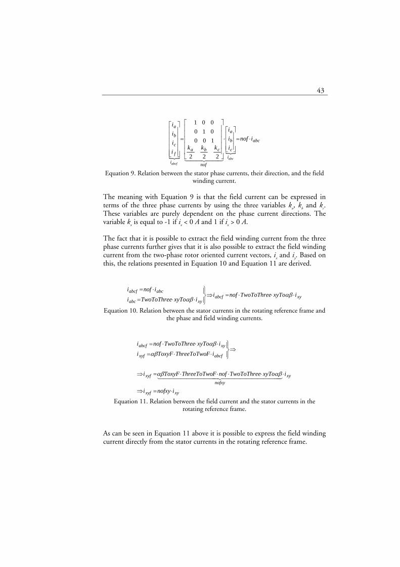
Equation 9. Relation between the stator phase currents, their direction, and the field winding current.
The meaning with Equation 9 is that the field current can be expressed in terms of the three phase currents by using the three variables ka, kb and kc. These variables are purely dependent on the phase current directions. The variable kx is equal to -1 if ix < 0 A and 1 if ix > 0 A.
The fact that it is possible to extract the field winding current from the three phase currents further gives that it is also possible to extract the field winding current from the two-phase rotor oriented current vectors, ix and iy. Based on this, the relations presented in Equation 10 and Equation 11 are derived.
xyabcfxyabc
abcabcfixyToTwoToThreenofi
ixyToTwoToThreei
inofi⋅⋅⋅=⇒
⎪⎭
⎪⎬⎫
⋅⋅=
⋅=αβ
αβ
Equation 10. Relation between the stator currents in the rotating reference frame and the phase and field winding currents.
xyxyf
xynofxy
xyf
abcfxyf
xyabcf
inofxyi
ixyToTwoToThreenofFThreeToTwoToxyFi
iFThreeToTwoToxyFi
ixyToTwoToThreenofi
⋅=⇒
⋅⋅⋅⋅⋅=⇒
⇒⎪⎭
⎪⎬⎫
⋅⋅=
⋅⋅⋅=
4444444444 34444444444 21 αβαβ
αβ
αβ
Equation 11. Relation between the field current and the stator currents in the rotating reference frame.
As can be seen in Equation 11 above it is possible to express the field winding current directly from the stator currents in the rotating reference frame.

44 Chapter 5. Modelling the SMSM
By multiplication of the transformation-matrixes used in Equation 11 the nofxy matrix that contains the diode bridge conduction variables ka,b,c and the instantaneous angular position of the rotor, θr, is revealed. The nofxy matrix is shown in Equation 12 below.
cbcba kkkandkkkkwith
kkkknofxy
−=−−⋅=
⎥⎥⎥⎥⎥
⎦
⎤
⎢⎢⎢⎢⎢
⎣
⎡
⋅⋅
−⋅⋅
⋅⋅
+⋅⋅
=
221
)sin(62
1)cos(22
210
)sin(22
2)cos(62
101
θθθθ
Equation 12. Revealing of the nofxy matrix.
Using the nofxy matrix it is possible to compress the voltage equation, Equation 8, even more. This is done in Equation 13.
( ) xyredxyfredxyred
xy
L
xyfxy
L
xyfxy
R
xyfxyf
iLiLdtdiR
inofxyLinofxyLdtdinofxyRu
redredred
rrr
r
43421
r
43421
r
43421
r
⋅⋅Ω+⋅+⋅=
⋅⋅⋅Ω+⎟⎟⎟
⎠
⎞
⎜⎜⎜
⎝
⎛⋅⋅+⋅⋅=
Equation 13. Compression of the voltage equation.
The Rred and Lred matrixes are presented below in Equation 14.

45
( ) ( )
( )
( )⎥⎥⎥⎥⎥⎥
⎦
⎤
⎢⎢⎢⎢⎢⎢
⎣
⎡
⋅−⋅⋅⋅⋅
⋅−⋅⋅⋅⋅
⋅⋅
⋅+⋅
⋅
⋅+
⋅⋅
⋅+⋅
⋅
⋅+
=
⎥⎥⎥⎥⎥⎥
⎦
⎤
⎢⎢⎢⎢⎢⎢
⎣
⎡
⋅⋅−⋅⋅⋅⋅
⋅⋅+⋅⋅⋅
=
)sin(1)cos(2362
)sin(1)cos(2362
)sin(22
2)cos(
62
10
)sin(22
2)cos(
62
1
)sin(1)cos(2362
0
)sin(23)cos(162
0
θθ
θθ
θθ
θθ
θθθθ
kkL
L
kkL
kLkLL
LkLkL
L
kkR
R
kkR
RR
f
sy
mf
ffmf
mfmfsx
red
fs
f
s
red
Equation 14. The Rred and Lred matrixes.
From the matrixes presented in Equation 14 two interesting discoveries are made.
Resistance matrix
• The resistances in x- and y-direction are still only depending on the stator resistances.
• The resistance of the field winding relation is also depending on diode bridge conduction state and the rotor electrical angular position.
Inductance matrix
• It is clear that the inductance in the x-direction is depending on the diode bridge conduction state and the electrical angular position.
• The inductance in the y-direction is not influenced.
• The inductance in the field winding is depending on the diode bridge conduction state and the electrical angular position. The stator x-directed inductance and the field winding inductance are coupled through the mutual inductance.


Chapter 6 Development of a simulation model of the SMSM
The derived mathematical model of the SMSM, from the previous chapter, states a relation between the phase voltages and the phase currents of the SMSM. For being able to perform simulations of the machine in operation, the relation between the phase potentials and phase voltages also need to be known. This relation, including the diode bridge rectifier and field winding, will be derived in this chapter. The diodes in the bridge rectifier are considered as ideal components that give no voltage drop when conducting and ideally fast switching between conducting and blocking state.
Let us begin by reintroducing the most important figure in this thesis, Figure 3.4. There are 823 = different current flow direction configurations of three phase systems as can be seen in Table 3.
Table 3. Different current direction configurations.
ia ib ic ka kb kc <0 <0 <0 -1 -1 -1 <0 <0 >0 -1 -1 1 <0 >0 <0 -1 1 -1 <0 >0 >0 -1 1 1 >0 <0 <0 1 -1 -1 >0 <0 >0 1 -1 1 >0 >0 <0 1 1 -1 >0 >0 >0 1 1 1
This gives that the diode bridge rectifier will theoretically be able to be in eight different conducting states. Two of those can directly be left out by the
48 Chapter 6. Development of a simulation model of the SMSM
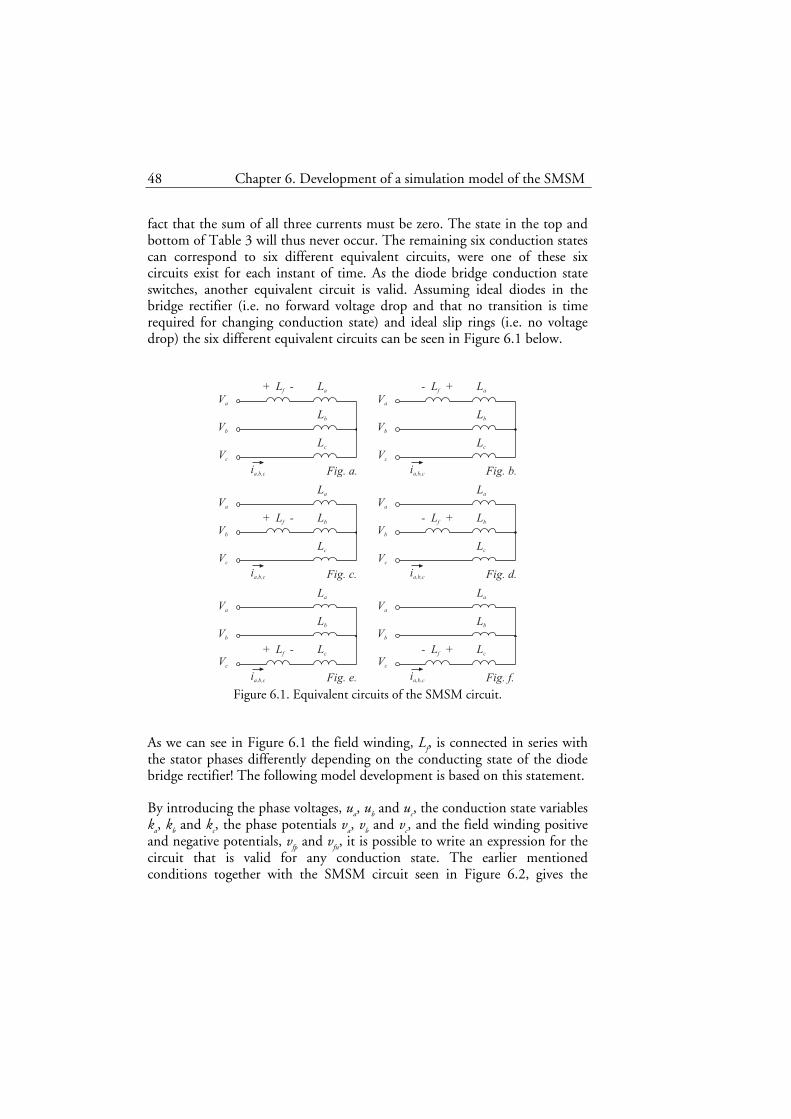
fact that the sum of all three currents must be zero. The state in the top and bottom of Table 3 will thus never occur. The remaining six conduction states can correspond to six different equivalent circuits, were one of these six circuits exist for each instant of time. As the diode bridge conduction state switches, another equivalent circuit is valid. Assuming ideal diodes in the bridge rectifier (i.e. no forward voltage drop and that no transition is time required for changing conduction state) and ideal slip rings (i.e. no voltage drop) the six different equivalent circuits can be seen in Figure 6.1 below.
La
ia,b,c
Va
Vb
Vc
+ L -f
Lb
Lc
Fig. a.
La
ia,b,c
Va
Vb
Vc
- L +f
Lb
Lc
Fig. b.
La
ia,b,c
Va
Vb
Vc
+ L -f Lb
Lc
Fig. c.
La
ia,b,c
Va
Vb
Vc
- L +f Lb
Lc
Fig. d.
La
ia,b,c
Va
Vb
Vc
+ L -f
Lb
Lc
Fig. e.
La
ia,b,c
Va
Vb
Vc
- L +f
Lb
Lc
Fig. f. Figure 6.1. Equivalent circuits of the SMSM circuit.
As we can see in Figure 6.1 the field winding, Lf, is connected in series with the stator phases differently depending on the conducting state of the diode bridge rectifier! The following model development is based on this statement.
By introducing the phase voltages, ua, ub and uc, the conduction state variables ka, kb and kc, the phase potentials va, vb and vc, and the field winding positive and negative potentials, vfp and vfn, it is possible to write an expression for the circuit that is valid for any conduction state. The earlier mentioned conditions together with the SMSM circuit seen in Figure 6.2, gives the

49
circuit potential relations of the SMSM that are shown in Equation 15.
ua D1
D4
D3 D5
D6 D2
ia,b,c
va
vb
vc
vfp
Sliprings
ub
uc vfn
Figure 6.2. The SMSM circuit.
⎥⎦
⎤⎢⎣
⎡⋅
⎥⎥⎥⎥⎥⎥
⎦
⎤
⎢⎢⎢⎢⎢⎢
⎣
⎡
−−
−−
−−
+
+
+
−⎥⎥⎥
⎦
⎤
⎢⎢⎢
⎣
⎡=
⎥⎥⎥⎥⎥⎥
⎦
⎤
⎢⎢⎢⎢⎢⎢
⎣
⎡
−⋅+
+⋅−
−⋅+
+⋅−
−⋅+
+⋅−
=⎥⎥⎥
⎦
⎤
⎢⎢⎢
⎣
⎡
fn
fp
c
b
a
c
b
a
c
b
a
cfn
cfpc
bfn
bfpb
afn
afpa
c
b
a
vv
k
k
k
k
k
k
vvv
kv
kvv
kv
kvv
kv
kvv
uuu
21
21
21
21
21
21
21
21
21
21
21
21
Equation 15. The SMSM circuit potential relations.
The fact that the three phase voltages still form a symmetric system,
0=++ cba uuu , and that the field voltage fu can be expressed in the field potentials, fnfpf vvu −= , gives the opportunity to continue developing the result of Equation 15. In Equation 16 a relation between the field winding voltage and the circuit potentials are shown.
⎥⎦
⎤⎢⎣
⎡++
=⎥⎦
⎤⎢⎣
⎡⋅
⎥⎥⎦
⎤
⎢⎢⎣
⎡−+++++
−
⇒⎪⎭
⎪⎬
⎫
−=
−++⋅−
+++⋅=++⇒
=−
⋅++
⋅−
+−
⋅++
⋅−+−
⋅++
⋅−=++
cba
f
fn
fpcbacba
fnfpf
cbafn
cbafpcba
u
cfn
cfpc
u
bfn
bfpb
u
afn
afpacba
vvvu
vv
kkkkkk
vvu
kkkv
kkkvvvv
kv
kvv
kv
kvv
kv
kvvuuu
c
ba
23
23
11
23
23
02
12
1
21
21
21
21
4444 34444 21
4444 34444 2144444 344444 21
Equation 16. Relation between field winding voltage and circuit potentials.

50 Chapter 6. Development of a simulation model of the SMSM
Using Equation 15 and Equation 16 it is possible to eliminate the field voltage potentials, vfp and vfn, and express the phase voltages from the field winding voltage, phase potentials and diode bridge conduction state constants as Equation 17.
f
k
abc
cab
cba
u
abc
cab
cba
cba
fcbacba
c
b
a
c
b
a
c
b
a
c
b
a
u
kkk
kkk
kkk
vvv
vvv
vvv
vvvukkkkkk
k
k
k
k
k
k
vvv
uuu
virtabc
⋅
⎥⎥⎥⎥⎥⎥
⎦
⎤
⎢⎢⎢⎢⎢⎢
⎣
⎡
−−
−−
−−
−
⎥⎥⎥⎥⎥⎥
⎦
⎤
⎢⎢⎢⎢⎢⎢
⎣
⎡
−−
−−
−−
=
⎥⎦
⎤⎢⎣
⎡++
⋅⎥⎥⎦
⎤
⎢⎢⎣
⎡−++
−+++⋅
⎥⎥⎥⎥⎥⎥
⎦
⎤
⎢⎢⎢⎢⎢⎢
⎣
⎡
−−
−−
−−
+
+
+
−⎥⎥⎥
⎦
⎤
⎢⎢⎢
⎣
⎡=
⎥⎥⎥
⎦
⎤
⎢⎢⎢
⎣
⎡ −
44 344 2144 344 214,
62
62
62
32
32
32
23
1
23
1
21
21
21
21
21
21
1
Equation 17. Relation between the phase voltages, circuit potentials and field winding voltage.
Notice the two voltage vectors introduced in Equation 17, uabc,virt and k4. The outcome from Equation 17 is, when looking closer, not very surprising. The virtual voltage vector, uabc,virt, reflects the voltage vector that would occur if dealing with an ordinary star-connected three-phase AC machine! The difference, from using an ordinary star-connected three-phase AC machine, is that the field voltage is subtracted from the voltage vector in the actual phase. As mentioned before, the field winding is connected in series with one of the three stator phases. (As Figure 6.1 shows) The field voltage is subtracted from the correct phase by the use of the k4 matrix.
Notice that the previous mathematics in this chapter is valid for the abc reference frame. From here and on, transformations are performed so that the model will be valid for the rotor oriented reference frame.
Equation 17 is first transformed into the non-rotating two-dimensional reference frame (αβ) and then further to the rotating two-dimensional reference frame (xy) resulting in Equation 18.

51
fxyvirtxyfk
virtxyxy ukuukThreeToTwoToxyuuxy
⋅−=⋅⋅⋅−= 3,4,
3
4444 34444 21αβ
Equation 18. Transformation of the field voltage to the rotating reference frame.
Yet, another term is introduced, k3xy, that transforms the one-dimensional field winding voltage quantity, uf, to the rotating two-dimensional field voltage vector is introduced. An interpretation of the k3xy matrix in Equation 18 is that the field winding voltage is added to the, for the instant, correct phase and then transformed to the xy-frame, via the αβ -frame, were its voltage is added to the stator winding voltage. The k3xy matrix can be viewed in Equation 19.
⎥⎥⎥⎥
⎦
⎤
⎢⎢⎢⎢
⎣
⎡
⋅−⋅
⋅+⋅⋅=
)sin(62
1)cos(22
2
)sin(22
2)cos(62
1
3θθ
θθ
kk
kk
k xy
Equation 19. The k3xy matrix.
Figure 6.3 can be used as a visualization aid of Equation 18. The applied voltage vector uxy,virt is shared between the stator voltage vector, uxy, and the field voltage vector, ufxy.
x
y
uxy
uxy,virt
u =u*k3xyfxy f
Figure 6.3. Field-, stator- and applied voltage vector relation.
Since the k3xy matrix contain the diode bridge conduction state, that change
52 Chapter 6. Development of a simulation model of the SMSM
values abruptly, the xyfur vector will also move transiently in the xy reference
frame. Figure 6.3 shows only the principles of Equation 18.
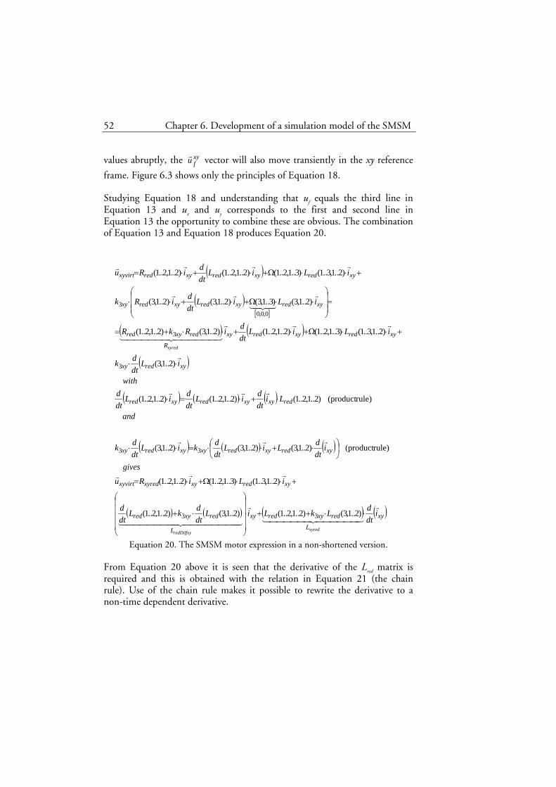
Studying Equation 18 and understanding that uf equals the third line in Equation 13 and ux and uy corresponds to the first and second line in Equation 13 the opportunity to combine these are obvious. The combination of Equation 13 and Equation 18 produces Equation 20.
( )
( )[ ]
( ) ( )
( )
( ) ( ) ( )
( ) ( ) ( )
( ) ( ) ( ) ( )xy
L
redxyredxy
L
redxyred
xyredxyxyredxyvirt
xyredxyredxyxyredxy
redxyxyredxyred
xyredxy
xyredxyredxy
R
redxyred
xyredxyredxyredxy
xyredxyredxyredxyvirt
idtdLkLiL
dtdkL
dtd
iLiRu
gives
idtdLiL
dtdkiL
dtdk
and
LidtdiL
dtdiL
dtd
with
iLdtdk
iLiLdtdiRkR
iLiLdtdiRk
iLiLdtdiRu
xyredredDiffxy
xyred
r
444444 3444444 21
r
44444444 344444444 21
rrr
rrr
rrr
r
rrr
444444 3444444 21
r
43421
rr
rrrr
⋅⋅++⋅
⎟⎟⎟⎟
⎠
⎞
⎜⎜⎜⎜
⎝
⎛
⋅+
+⋅⋅Ω+⋅=
⎟⎠⎞
⎜⎝⎛ ⋅+⋅⋅=⋅⋅
⋅+⋅=⋅
⋅⋅
+⋅⋅Ω+⋅+⋅⋅+=
=⎟⎟⎟
⎠
⎞
⎜⎜⎜
⎝
⎛⋅⋅Ω+⋅+⋅⋅
+⋅⋅Ω+⋅+⋅=
⋅ )2..1,3()2..1,2..1()2..1,3()2..1,2..1(
)2..1,3..1()3..1,2..1()2..1,2..1(
rule)(product )2..1,3()2..1,3()2..1,3(
rule)(product )2..1,2..1()2..1,2..1()2..1,2..1(
)2..1,3(
)2..1,3..1()3..1,2..1()2..1,2..1()2..1,3()2..1,2..1(
)2..1,3()3..1,3()2..1,3()2..1,3(
)2..1,3..1()3..1,2..1()2..1,2..1()2..1,2..1(
33
33
3
3
0,0,03
Equation 20. The SMSM motor expression in a non-shortened version.
From Equation 20 above it is seen that the derivative of the Lred matrix is required and this is obtained with the relation in Equation 21 (the chain rule). Use of the chain rule makes it possible to rewrite the derivative to a non-time dependent derivative.

53
( ) ( ) ( ) ( ) redDiffredelredred LLdd
dtdL
ddL
dtd
=⋅=⋅=θ
ωθθ
Equation 21. Applying the chain rule.
The derivative of Lred (see Equation 14) with respect to the angle, θr, is more or less easy to derive analytically and is here named LredDiff. The LredDiff matrix is presented below in Equation 22.
( )
( )⎥⎥⎥⎥⎥⎥
⎦
⎤
⎢⎢⎢⎢⎢⎢
⎣
⎡
⋅+⋅⋅⋅⋅
−
⋅+⋅⋅⋅⋅
−
⋅⋅
⋅+⋅
⋅
⋅−
⋅⋅
⋅+⋅
⋅
⋅−
= ⋅
)cos(1)sin(2362
0
)cos(1)sin(2362
)cos(22
2)sin(
62
10
)cos(22
2)sin(
62
1
θθ
θθ
θθ
θθ
ω
kkL
kkL
kLkL
LkLk
Lf
mf
ff
mfmf
elredDiff
Equation 22. The LredDiff matrix.
As we see now there is an expression that relates the current in the xy-reference frame to the voltage in the xy-reference frame taking the field winding into account at the same time! In the simulation, it is desirable to be able to apply a certain set of phase voltage potentials and then see what currents are driven. In Equation 23, Equation 20 is rewritten so that it is useful for simulation.
( )( )dtiLiLiRuLi xyredDiffxyxyredxyxyredxyvirtxyredxy ∫ ⋅−⋅⋅Ω−⋅−⋅= − rrrrr)2..1,3..1()3..1,2..1(1
Equation 23. SMSM current and voltage relations suitable for performing simulations.
Results from simulations in Matlab Simulink utilizing the mathematical model presented in Equation 23 are presented later in Chapter 8, page 65.


Chapter 7 Control methods
In this chapter, the first two sections presents two different current control methods operating in the rotating reference frame. The third subchapter presents a method that helps a SMSM to produce a smooth torque.
7.1 Dedicated vector based current controller
In this section, current-controllers controlling the x- and y-directed currents in a SMSM are derived outgoing from the model that is derived for the SMSM. The method for deriving the controllers follows the methodology presented in literature by Alaküla M. (2002).
Control of a SMSM utilizing dedicated current controllers is expected to reach higher performance than control based on standard PI controllers.
The derivation of the current controllers is assumed to apply Dead Beat Control. The principle of Dead Beat Control is to find the controller output that must be applied to a system in order to bring the system output to the set point in a minimum number of time steps. Ideally, the controller needs only one time step (i.e. one sample interval) to reach the set point.
The controllers that are derived are supposed to be implemented digitally in a Digital Signal Processor, DSP. The starting-point in the derivation is Equation 20. Averaging Equation 20 oven one sample-time period, Ts, gives Equation 24.

56 Chapter 7. Control methods
( )
( )dtidtdL
TdtiL
T
dtiLT
dtiRT
dti
dtdLiL
iLiRdtu
T
s
s
s
s
s
s
s
s
s
ss
Tk
Tkxyxyred
s
Tk
TkxyredDiffxy
s
Tk
Tk
Tk
Tkxyred
sxyxyred
s
Tk
Tk xyxyredxyredDiffxy
xyredxyxyredTsk
Tkxyvirt
s
∫∫
∫ ∫
∫∫
⋅+
⋅
⋅+
⋅
⋅+
⋅
⋅+
⋅
⋅+
⋅
⋅+
⋅
⋅+⋅
+⋅⋅Ω+⋅=
=⎟⎟⎟
⎠
⎞
⎜⎜⎜
⎝
⎛
⋅+⋅
+⋅⋅Ω+⋅=
)1()1(
)1( )1(
)1()1(
11
)3..1,2..1()3..1,2..1(11
)2..1,3..1()3..1,2..1(1
rr
rr
rr
rr
r
Equation 24. Average of the SMSM equation over one sample time period.
A number of approximations are introduced and shown below. Presumptions:
a.) [ ] ( )kukku xyvirtxyvirt
∗=+rr
1,
b.) ( ) ( )kiki xyxy∗=+
rr1
c.) [ ] ( ) ( )2
1,kiki
kki xyxyxy
rrr +
=+∗
d.) ( ) ( ) ( )∑−=
=
∗ −=1
0
kn
nxyxyxy ninikirrr
e.)
( ) ( )
( ) ( )( ) ( )( ) ( )
⎪⎪⎪⎪
⎩
⎪⎪⎪⎪
⎨
⎧
+≈
+≈
+≈+≈
+≈+≈+Ω≈Ω
)1()(
1
11
)1()()1()(..1
kLkL
kLkL
kRkRkLkL
kkkkeikk
redDiffxyredDiffxy
xyredxyred
xyredxyred
redred
θθωω
Equation 25. Introduced approximations.
The star (*) that appears in Equation 25 denotes that the value is a set-point value for the controller.
Below follows explanations for the previously introduced presumptions in

7.1. Dedicated vector based current controller 57
Equation 25.
a.) The average value over one sample period of the output voltage vector is equal to the set-point of the voltage vector.
b.) The controller manages to control the current within one sample time interval. This presumption implies that the voltage source has an unlimited voltage level so that the desired current is reached within one sample interval.
c.) Presumption c.) is a consequence of presumption b.). The average value of the x- and y-currents in the time interval [ ]1, +kk equals the mean value of the set-point value (that is equal to next time instant value according to b.) and the actual x- and y-currents. This means that the current is changing approximately linearly in the interval.
d.) Since we are assuming that the set-point is reached within one sample interval, the sum of all changes in each sample-time interval in the x- and y-directed currents equals the actual currents.
e.) The rotational speed-, the reduced resistance- and the inductance matrixes do not change considerably during the short sample interval. This is of course an approximation as well and implies that the controller will not be ideal. This probably introduces errors similar to the behaviour of the parameter variations present in the rotating machine.
Utilizing the approximations mentioned above leads further in the development of the dedicated xy-current controller.
Presumption a.), b.), c.) and e.) above make it possible to move the parameter matrixes outside the integral signs as follows in Equation 26.

58 Chapter 7. Control methods
[ ] ( ) ( ) ( ) ( )
( ) ( )
( )( ) ( )
44 344 21
r
44 344 21
r
44 344 21
r
44 344 21
r
44 344 21
r
rrrr
rrrrr
kiki
Tk
Tkxy
sxyred
kiki
Tk
Tkxy
sredDiffxy
kiki
Tk
Tkxy
sred
kiki
Tk
Tkxy
sxyred
kku
Tsk
Tkxyvirt
s
xyxy
s
s
xyxy
s
s
xyxy
s
s
xyxy
s
s
xy
s
dtidtd
TLdti
TL
dtiT
LdtiT
RdtuT
−
⋅+
⋅
+
⋅+
⋅
+
⋅+
⋅
+
⋅+
⋅
+
⋅+
⋅
∗∗
∗∗
∫∫
∫∫∫
⋅+⋅
+⋅⋅Ω+⋅=
)1(
2
)1(2
)1(
2
)1(
1,
)1(
11
1)3..1,2..1()3..1,2..1(11
Equation 26. Insertion of presumptions a.), b.), c.) and e.).
Insertion and usage of presumption d gives Equation 27.
[ ] ( ) ( ) ( ) ( )
( ) ( )( ) ( )( )
( ) ( )( ) ( )( ) ( )
( )
( ) ( )
( )
( ) ( )( )
( ) ( ) ( )( )
( ) ( ) ( )( ) ( )4444 34444 21
r
4444444 34444444 21
rr
4444444 34444444 21
rrr
rr
44 344 21
rr
44 344 21
rrrrr
rrrr
rrrrr
r
r
EMFinduced i.e. part, forward Feedpart Integral
1
0
part alProportion
*
*
*
*
)3..1,2..1(
12
12
2)3..1,2..1(1
2
112
2)3..1,2..1(
21,
kiLniniLR
kikiT
LRku
kikiT
LkikiL
kikiLkiRkiki
R
kikiT
Lkiki
L
kikiL
kikiRkku
xyredkn
nxyxyredDiffxyxyred
xyxys
xyredxyredxyvirt
xyxys
xyred
ki
xyxyredDiffxy
ki
xyxyredxyxyredxyxy
xyred
xyxys
xyredxyxy
redDiffxy
xyxyred
xyxyxyredxyvirt
xy
xy
⋅⋅Ω+−⋅+
+−+⋅⎟⎟⎠
⎞⎜⎜⎝
⎛+=
⇒−+⋅++
⋅
++
⋅⋅Ω+⋅+−+⋅
=−+⋅⋅++
⋅
++
⋅⋅Ω++
⋅=+
∑−=
=
∗
∗
≈
∗
≈
∗
∗
∗∗
Equation 27. Insertion of presumption d and further development.
To estimate the control dynamics, some fictitious values and some data from an existing Series Magnetized Synchronous Machine, Hagstedt D (2004), are inserted into the derived controller algorithm (Equation 27). The data for the

7.1. Dedicated vector based current controller 59
evaluated SMSM is presented later in Table 4 at page 70. In Equation 28 a rough estimate of the controller output voltage reference is made.
Assuming 0 A as initial current both in the x- and y-direction, a y-direction current set point is 10 A, initial rotational speed is 0 rad/s, the terms in the matrixes Rxyred and Lxyred are approximated in Equation 28 (Estimations of average values obtained from simulations) and finally the sampling rate is fs=15 kHz. ( ss fT /1= is the sample-time, the time between each sampling instant)
( ) ( )( )
( ) ( ) ( )( ) ( )
⎥⎦
⎤⎢⎣
⎡=⎥
⎦
⎤⎢⎣
⎡⋅
⎟⎟⎟⎟⎟⎟⎟⎟⎟
⎠
⎞
⎜⎜⎜⎜⎜⎜⎜⎜⎜
⎝
⎛
⎥⎦
⎤⎢⎣
⎡
+⎥⎦
⎤⎢⎣
⎡
≈⋅⋅Ω+−⋅+
+−+⋅⎟⎟⎠
⎞⎜⎜⎝
⎛+=
≈≈
−=
=
∗
≠
∑
VV
AA
kiLniniLR
kikiT
LRu
s
s
xyred
xyred i
TL
R
xyredkn
nxyxyredDiffxyxyred
xyxys
xyredxyredxyvirt
105166001
100
150001
07.004.004.005.0
215.32.02.085.2
)3..1,2..1(
12
2
00
1
0
0
**
3214434421
4434421
4444 34444 21
r
4444444 34444444 21
rr
4444444 34444444 21
rrr
Equation 28. Estimation of the controller output values.
The estimated voltage reference is of course not a feasible voltage-level for this application, if ever. From this, it is understood that the actual set-point value will not be reached within one sample time interval for the specified sampling rate. Yet, this assumption is used for reaching the final current controller structure. A very brief estimation of the shortest possible current settling-time (time to reach the set-point value) using the same parameters as used in Equation 28 but with 300 V DC-link voltage, indicates a current settling time (0-10 A) of at least 2.5 ms. The dynamics of the system is thus specified by the DC-link voltage and the specific machine properties. For reaching control stability, the sampling rate should be at least 8-10 times faster than the dynamics of the system to be controlled. The reasoning above implies that it is not possible to perform any changes in the xy-reference frame that are faster than the system dynamics. This sets an upper bandwidth limit on the

60 Chapter 7. Control methods
torque compensating method that is presented later on. Nevertheless, a high sample rate is required for updating the controllers with the correct rotor position at high rotational speeds. The sampling of the phase currents is synchronized with the converter switching for collecting current measurements that do not contain any current ripple resulting from the switching.
It is possible to separate the x and y variable by separating the lines in the current controller algorithm that is presented in Equation 27, this is done in Equation 29.
( ) ( )( )
( ) ( ) ( )( ) ( )
( ) ( )( )
( ) ( ) ( )( ) ( )⎪⎪⎪⎪⎪⎪
⎩
⎪⎪⎪⎪⎪⎪
⎨
⎧
⋅⋅Ω+−⋅+
+−⋅⎟⎟⎠
⎞⎜⎜⎝
⎛+=
⋅⋅Ω+−⋅+
+−⋅⎟⎟⎠
⎞⎜⎜⎝
⎛+=
∑
∑
−=
=
∗∗
∗
−=
=
∗∗
∗
1
0
*
1
0
*
)1,3..2()3..1,2()2..1,2()2..1,2(
)2..1,2(2
)2..1,2()(
)1,3..1()3..1,1()2..1,1()2..1,1(
)2..1,1(2
)2..1,1()(
kn
nyredyyredDiffxyxyred
yys
xyredxyredyvirt
kn
nxredxxredDiffxyxyred
xxs
xyredxyredxvirt
kiLniniLR
kikiT
LRku
kiLniniLR
kikiT
LRku
Equation 29. Control algorithms for the x and y direction respectively.
Simulation results utilizing this controller are presented in Chapter 8.3 at page 76.
7.2 Field voltage vector feed forward
As the diode bridge rectifier forces a reconfiguration of the SMSM circuit at each change of conduction state, the field winding is connected in different ways as earlier shown in Figure 6.1. The field voltage vector shown in Figure 6.3 thus adds upon the stator voltage vector. The transient changes, arising from the circuit reconfigurations, introduce high demands on the performance of the current control of the SMSM. As the field voltage vector is predictable, since we have the model of the SMSM, there is an opportunity to calculate this voltage vector and feed it forward onto the output of the controller. Hereby the controller is helped to compensate for the otherwise cumbersome voltage transients introduced by the circuit reconfigurations.

7.3. Torque compensation 61
The reasoning above is a simple approach to obtain controllers that are structurally simpler than the dedicated controllers are but still are aware of the voltage transients.
Simulation results evaluating this type of controller are presented in section 8.4 at page 81.
7.3 Torque compensation
In the simulation results, it is realized that the torque, generated by a SMSM, may not be as smooth as from an EMSM. Applying a constant current set-point level in the y-direction normally gives a constant produced torque from Synchronous Machines. In the SMSM case the field current is not constant and thus neither the generated field flux. (Because iL⋅=Ψ ) The generated torque depends on the generated field flux and the stator current according to
ssel iT ×Ψ= . The torque ripple produced by a SMSM is approximately 15 % out of the total produced torque, which agree with previous results, Tonin D. (2003)
For eliminating this undesired torque ripple, an additional control algorithm is applied for compensating the x- and y-direction current set-points. This additional algorithm has the input quantity torque and the output quantity corresponding to a current set-point. Mostly it is of minor importance that the input torque set-point equals the generated torque since the drive in many cases is speed controlled and thereby consists of two cascaded control loops where the inner loop is the current/torque controller and the outer is the speed controller. Both the inner and the outer controller are often of proportional and integral type and therefore the outer controller demands enough torque for reaching the speed set-point.
The torque compensation algorithm presented here is straightforward. The deduction begins from the relation between the x- and y -direction current and the produced fluxes in each direction. The relationship is shown in the first line in Equation 30. The flux-linkage in the stator x-direction consists of flux-linkage from the field winding via the mutual inductance and the flux generated in the stator x-direction itself. (Line three in Equation 30) The flux-linkage in the y-direction consists from the flux generated in the stator y-direction itself only. (Line four in Equation 30) Adding these facts leads to the expression for the generated torque that is shown in the last line of Equation 30.
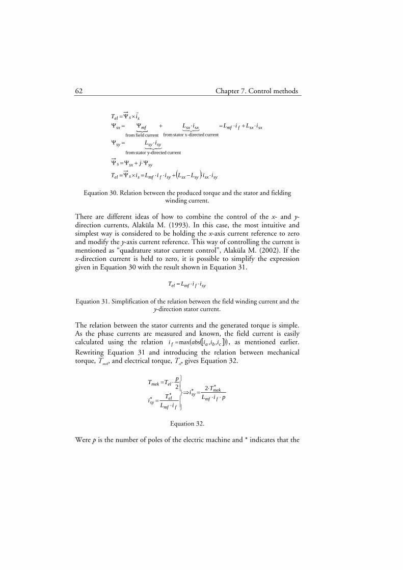
62 Chapter 7. Control methods
( ) sysxsysxsyfmfssel
sysxs
sysysy
sxsxfmfsxsxmfsx
ssel
iiLLiiLiT
j
iL
iLiLiLiT
⋅⋅−+⋅⋅=×Ψ=
Ψ⋅+Ψ=Ψ
⋅=Ψ
⋅+⋅=⋅+Ψ=Ψ×Ψ=
321
321
r
current directed-stator y from
current directed-xstator fromcurrent field from
Equation 30. Relation between the produced torque and the stator and fielding winding current.
There are different ideas of how to combine the control of the x- and y-direction currents, Alaküla M. (1993). In this case, the most intuitive and simplest way is considered to be holding the x-axis current reference to zero and modify the y-axis current reference. This way of controlling the current is mentioned as “quadrature stator current control”, Alaküla M. (2002). If the x-direction current is held to zero, it is possible to simplify the expression given in Equation 30 with the result shown in Equation 31.
syfmfel iiLT ⋅⋅=
Equation 31. Simplification of the relation between the field winding current and the y-direction stator current.
The relation between the stator currents and the generated torque is simple. As the phase currents are measured and known, the field current is easily calculated using the relation [ ]( )( )cbaf iiiabsi ,,max= , as mentioned earlier. Rewriting Equation 31 and introducing the relation between mechanical torque, Tmek, and electrical torque, Tel, gives Equation 32.
piLT
i
iLT
i
pTT
fmf
meksy
fmf
elsy
elmek
⋅⋅⋅
=⇒
⎪⎪⎭
⎪⎪⎬
⎫
⋅=
⋅=∗
∗∗
∗
22
Equation 32.
Were p is the number of poles of the electric machine and * indicates that the

7.3. Torque compensation 63
value is a set point value.
The y-directed current set point output is expected to act like the inverse of the field current ripple that also can be seen in the results in Chapter 8.5 at page 85.


Chapter 8 Simulation results
8.1 Implementation of simulation model
In this chapter, the control algorithms from earlier chapters are implemented in the graphical simulation environment Matlab Simulink. The simulation results are presented in the same order as in previous chapters. In the first section, simulation results from simulating the operation of a SMSM controlled by a common PI vector controller with the x- and y-direction currents as the controlled quantities. Next subchapter presents the results from operating the SMSM with, for the SMSM, dedicated current controllers. In subchapter three simulation results from controlling the SMSM with the voltage vector feed forward control method are presented.
When studying the simulation results and realizing that the current in y-direction is no longer almost proportional to the generated torque, as in the case of other types of synchronous machines. The controller is further extended with a torque compensator, as mentioned earlier. These simulation results are presented in the fourth subchapter.
The top level of the simulation model is shown in Figure 8.1.

66 Chapter 8. Simulation results
Figure 8.1. Top level of simulation model.

8.1. Implementation of simulation model 67
In Figure 8.1 the commonly used vector controller structure is shown. The stator phase currents are measured on the three phase electric machine (on the right) and fed into the vector controller block (on the left).
In the simulation model shown above, the controller block transforms, by using the angular position of the rotor, the actual current vector (in the αβ reference frame) further to the rotating xy reference frame. In the xy reference frame, the actual values are compared to the set-point values that also are fed into the vector controller block. The PI controller is then operating based on the deviation between set-point values and actual current values.
The controller calculates a suitable voltage vector that is required for reaching the set-point current. The required voltage vector is then transformed back to the three-phase reference frame via the two-dimensional non-rotating reference frame.
After the controller block, the “modulation method” block calculates corresponding phase set-point voltages by using different modulation algorithms. The different modulation methods that are implemented are Sinus modulation, Symmetrized modulation and Minimum switching modulation. Depending on which modulation method that is chosen, different switching patterns are applied to the machine.
The group of seven blocks in the bottom right of Figure 8.1 is for saving data for further data analysis.
The power electronic dynamics are excluded from the simulation for speeding up the simulation but it is verified, by testing, that the result when including and excluding power electronics are similar.
Results from Chapter 6 and Equation 23 gives the graphical model for the SMSM that is implemented in the block “Three phase Electric Machine” in Figure 8.1. The simulation model of the SMSM is shown in Figure 8.2.

68 Chapter 8. Simulation results
Figure 8.2. The model of the SMSM.

8.1. Implementation of simulation model 69
The model for the SMSM, shown in Figure 8.2, may seem complicated to follow but since it is built up strictly following the Series Magnetized Synchronous Machine expression, Equation 23, it is considered to need no deeper explanation.
The main difference between this model and an Electrically Magnetized Synchronous Machine is that the machine impedances are depending on the diode bridge conduction state and thus the rotor position. All varying properties of the machine are calculated in the “Impedance Matrix” block, seen in Figure 8.2. In this block also the inverse and derivative of the Lredxy matrix is calculated.
In the following, results from simulations are studied. As the model does not contain a speed controller, it should be observed that a constant y-direction current will result in an accelerating or decelerating torque depending on the sign of the current. In the simulated case, a step of 10 A in the y-direction and 0 A in the x-direction is applied to the set-point of the current controller at the time of 1 ms. At 30 ms the y-direction set-point value is decreased to 1 A. The x-direction current reference is kept to 0 A during the simulation. The initial mechanical angular speed of the machine is 40 rad/s. The sample frequency, fs, is chosen to 15 kHz and the DC-link voltage is set to 300 V. The load torque is set to 5 Nm and the inertia of the rotor, J , is assumed to be 0.02 kgm2. The modulation method that is applied during the simulations is sinus modulation. The high sampling frequency is based on the maximum rotational speed of 18000 rpm and a 12 pole machine. 15 kHz is fast enough for performing 8.3 samples per electrical period that is assumed to be on the lower limit for control.
Table 4 shows the electric machine parameters achieved from experiments on the modified Lundell Generator, originally rated to 140 A, 14 V according to Bosch, referred to in Hagstedt D. (2004).

70 Chapter 8. Simulation results
Table 4. Properties of the SMSM available in the laboratory.
Description Symbol Value Unit Stator inductance in x - direction Lsx 24.3 mH Stator inductance in y - direction Lsy 27.5 mH Field winding inductance Lmf 30.8 mH Stator resistance Rs 2.8 Ω Field winding resistance Rf 0.65 Ω Number of poles p 12 poles Rotor inertia J 0.08 kgm2
As a complement to the different simulated controllers, controller output voltage level limitation and anti-windup are introduced according to Figure 8.3 and Figure 8.4.
Figure 8.3. Anti-windup for controller.

8.2. SMSM controlled by standard SM PI controllers 71
Figure 8.4. Output limitation for controller.
The saturation block in Figure 8.4 limits the signal between one and infinity.
8.2 SMSM controlled by standard SM PI controllers
As we can see in Figure 8.5, the field current equals max(abs(ia,ib,ic)) as expected. The phase current has a sinusoidal, but not perfectly sinusoidal shape.
In Figure 8.6 the set-point and the actual values of the currents in the xy reference frame are shown. From Figure 8.6, it is clear that the commutations of the diode bridge rectifier introduce challenges for the PI controllers. At each commutation, the machine impedances and thereby currents changes transiently. In the common case, controlling other types of Synchronous Machines, the PI controllers are handling DC signals in the rotating xy reference frame. In this case, also transients need to be taken into account, at least for perfect control. From Figure 8.6 it is obvious that there exist a cross connection between the x- and y direction currents. According to the discussion on page 59, it is clear that it is not possible to reach the set-point within one sample interval for such a set-point step that is applied.
The field current contains ripple and thus the generated torque contains ripple. The generated torque is calculated and shown together with the rotational speed in Figure 8.7. The torque ripple is theoretically calculated in Tonin D. (2003) to 15% that agrees with these simulation results.
The torque ripple may cause vibration in the driveline especially if the inertia and load torque is low but it is shown in Figure 8.7 that the consequences of the ripple are hardly noticeable in the plot of the rotational speed. (Even if this case is a low load condition.) If the driveline consists of a belt this might be harmed in the long run or together with the vibrations generate oscillations in the driveline. For this application, assuming a vehicle, the

72 Chapter 8. Simulation results
environment is very harsh and the torque quality requirements are not very high since the ICE itself generates a torque containing large pulsations.
A close view of Figure 8.6 shows that the current dynamics are similar to the results from the discussion in section 7.1. The discussion led to a current rise-time of 2.5 ms and the simulation results shown in Figure 8.6 gives a current rise-time of 5 ms.
0 0.005 0.01 0.015 0.02 0.025 0.03 0.035 0.04 0.045 0.05-10
-8
-6
-4
-2
0
2
4
6
8
10
Time [s]
Cur
rent
[A]
Figure 8.5. Phase- (solid) and field winding (dashed) current.

8.2. SMSM controlled by standard SM PI controllers 73
0 0.01 0.02 0.03 0.04 0.05
-10
-5
0
5
10
Time [s]
Cur
rent
[A]
0 0.01 0.02 0.03 0.04 0.05
-10
-5
0
5
10
Time [s]
Cur
rent
[A]
Figure 8.6. x (left) and y-direction (right) current references (dashed) and actual
currents (solid).
0 0.01 0.02 0.03 0.04 0.050
2
4
6
8
10
12
14
16
18
20
Time [s]
Torq
ue [N
m]
0 0.01 0.02 0.03 0.04 0.05
40
42
44
46
48
50
Time [s]
Spee
d [ra
d/s]
Figure 8.7. Generated mechanical torque and rotor rotational speed.
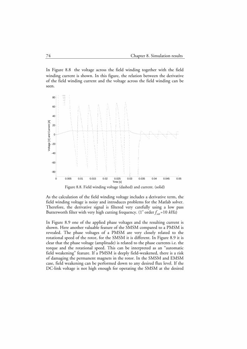
74 Chapter 8. Simulation results
In Figure 8.8 the voltage across the field winding together with the field winding current is shown. In this figure, the relation between the derivative of the field winding current and the voltage across the field winding can be seen.
0 0.005 0.01 0.015 0.02 0.025 0.03 0.035 0.04 0.045 0.05
-80
-60
-40
-20
0
20
40
60
80
Time [s]
Volta
ge [V
] and
Cur
rent
[A]
Figure 8.8. Field winding voltage (dashed) and current. (solid)
As the calculation of the field winding voltage includes a derivative term, the field winding voltage is noisy and introduces problems for the Matlab solver. Therefore, the derivative signal is filtered very carefully using a low pass Butterworth filter with very high cutting frequency. (1st order f3dB =10 kHz)
In Figure 8.9 one of the applied phase voltages and the resulting current is shown. Here another valuable feature of the SMSM compared to a PMSM is revealed. The phase voltages of a PMSM are very closely related to the rotational speed of the rotor, for the SMSM it is different. In Figure 8.9 it is clear that the phase voltage (amplitude) is related to the phase currents i.e. the torque and the rotational speed. This can be interpreted as an “automatic field weakening” feature. If a PMSM is deeply field-weakened, there is a risk of damaging the permanent magnets in the rotor. In the SMSM and EMSM case, field weakening can be performed down to any desired flux level. If the DC-link voltage is not high enough for operating the SMSM at the desired
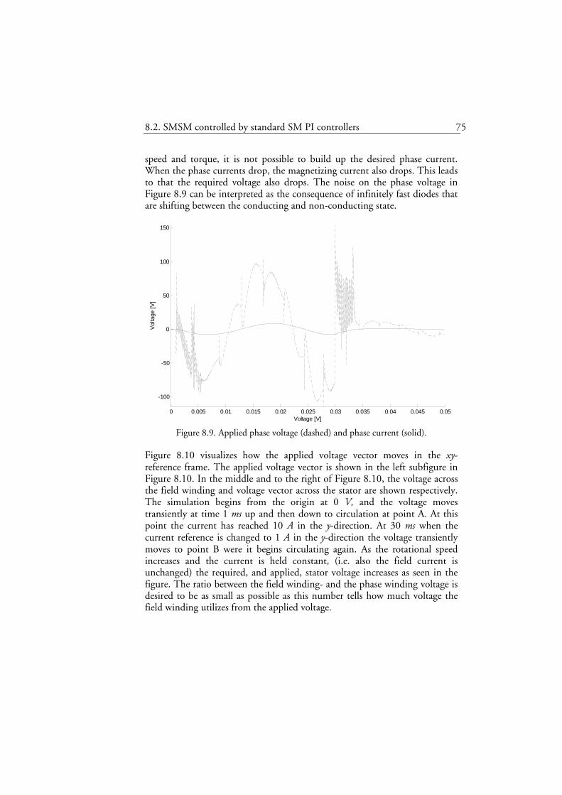
8.2. SMSM controlled by standard SM PI controllers 75
speed and torque, it is not possible to build up the desired phase current. When the phase currents drop, the magnetizing current also drops. This leads to that the required voltage also drops. The noise on the phase voltage in Figure 8.9 can be interpreted as the consequence of infinitely fast diodes that are shifting between the conducting and non-conducting state.
0 0.005 0.01 0.015 0.02 0.025 0.03 0.035 0.04 0.045 0.05
-100
-50
0
50
100
150
Voltage [V]
Volta
ge [V
]
Figure 8.9. Applied phase voltage (dashed) and phase current (solid).
Figure 8.10 visualizes how the applied voltage vector moves in the xy-reference frame. The applied voltage vector is shown in the left subfigure in Figure 8.10. In the middle and to the right of Figure 8.10, the voltage across the field winding and voltage vector across the stator are shown respectively. The simulation begins from the origin at 0 V, and the voltage moves transiently at time 1 ms up and then down to circulation at point A. At this point the current has reached 10 A in the y-direction. At 30 ms when the current reference is changed to 1 A in the y-direction the voltage transiently moves to point B were it begins circulating again. As the rotational speed increases and the current is held constant, (i.e. also the field current is unchanged) the required, and applied, stator voltage increases as seen in the figure. The ratio between the field winding- and the phase winding voltage is desired to be as small as possible as this number tells how much voltage the field winding utilizes from the applied voltage.

76 Chapter 8. Simulation results
-200 0 200-300
-200
-100
0
100
200
300Applied voltage vector
Voltage [v], x-direction
Volta
ge [v
], y-
dire
ctio
n
-200 0 200-300
-200
-100
0
100
200
300Voltage vector across field winding
Voltage [v], x-direction
Volta
ge [v
], y-
dire
ctio
n
-200 0 200-300
-200
-100
0
100
200
300Voltage vector across stator winding
Voltage [v], x-direction
Volta
ge [v
], y-
dire
ctio
nA
B AB
A
B
Figure 8.10. Voltage vectors in the rotating xy reference frame.
8.3 SMSM controlled by dedicated controller
In this subchapter, simulation results from controlling a SMSM utilizing the dedicated PI controller from 7.1 are presented. The SMSM properties, DC-link voltage, load torque, operating cycle, modulation method and sampling frequency are the same as in section 8.2. For being able to compare different results, the scope of the plots are the same as in section 8.2. After the result plots follows a discussion comparing the results.
0 0.005 0.01 0.015 0.02 0.025 0.03 0.035 0.04 0.045 0.05-10
-8
-6
-4
-2
0
2
4
6
8
10
Time [s]
Cur
rent
[A]
Figure 8.11. Phase current and field current.

8.3. SMSM controlled by dedicated controller 77
0 0.01 0.02 0.03 0.04 0.05
-10
-5
0
5
10
Time [s]
Cur
rent
[A]
0 0.01 0.02 0.03 0.04 0.05
-10
-5
0
5
10
Time [s]
Cur
rent
[A]
Figure 8.12. x (left) and y-directed (right) current references (dashed) and actual
currents (solid).
0 0.01 0.02 0.03 0.04 0.050
2
4
6
8
10
12
14
16
18
20
Time [s]
Torq
ue [N
m]
0 0.01 0.02 0.03 0.04 0.05
40
41
42
43
44
45
46
47
48
49
50
Time [s]
Spee
d [ra
d/s]
Figure 8.13. Generated mechanical torque (left) and rotor rotational speed.

78 Chapter 8. Simulation results
0 0.005 0.01 0.015 0.02 0.025 0.03 0.035 0.04 0.045 0.05
-80
-60
-40
-20
0
20
40
60
80
Time [s]
Volta
ge [V
] and
Cur
rent
[A]
Figure 8.14. Field winding voltage (dashed) and current (solid).
0 0.005 0.01 0.015 0.02 0.025 0.03 0.035 0.04 0.045 0.05
-150
-100
-50
0
50
100
150
Time [s]
Volta
ge [V
] and
cur
rent
[A]
Figure 8.15. Applied phase voltage (dashed) and phase current (solid).

8.3. SMSM controlled by dedicated controller 79
-200 0 200-300
-200
-100
0
100
200
300Applied voltage vector
Voltage [v], x-direction
Volta
ge [v
], y-
dire
ctio
n
-200 0 200-300
-200
-100
0
100
200
300Voltage vector across field winding
Voltage [v], x-directionVo
ltage
[v],
y-di
rect
ion
-200 0 200-300
-200
-100
0
100
200
300Voltage vector across stator winding
Voltage [v], x-direction
Volta
ge [v
], y-
dire
ctio
n
A
BA
B
A
B
Figure 8.16. Voltage vectors in the rotating xy reference frame.
A comparison between the corresponding plots utilizing different controllers follows.
There is no large difference between the phase- and field winding current waveforms (Figure 8.5 and Figure 8.11). What can be mentioned is that the phase current waveform is less sinusoidal for low currents when the dedicated current controllers are utilized.
The dynamics of the controllers in the rotating reference frame are studied and based on the results in Figure 8.6 and Figure 8.12. The current reference in the x- direction is held to zero and it is evident that the controller is not able to compensate for the cross-connection from the y-direction current step in any case of control method. It can also be concluded that the deviation from the set-point value is even larger using the dedicated controller in the x-direction. In the y-direction, the dedicated controller seems to be advantageous for treating the current ripple coming from the diode bridge commutations at high current levels. In low current levels, the dedicated controllers seem to perform worse. The overall performance in the rotating reference frame is similar for the two controllers.
Considering the generated mechanical torque in Figure 8.7 and Figure 8.13, only one difference is recognized. The difference is in the generated torque ripple, where the torque ripple is less when utilizing standard PI controllers.
As mentioned earlier, the current set-point will not be reached within one sample time interval when applying a step in the current set-point. By setting the DC-link voltage to a non-realistic value, 10 kV, and performing the same simulation again the transient miss-behaviour is almost erased. Such a high

80 Chapter 8. Simulation results
DC-link voltage equals an assumption that the voltage source is not a delimiting factor for reaching the current set-point within one sample time interval. This is shown in Figure 8.17. Utilizing such a high DC-link voltage is of course only possible in simulations and mainly interesting for investigating the reason of the miss-behaviour in transient mode of operation.
0 0.01 0.02 0.03 0.04 0.05
-10
-5
0
5
10
Time [s]
Cur
rent
[A]
0 0.01 0.02 0.03 0.04 0.05
-10
-5
0
5
10
Time [s]
Cur
rent
[A]
Figure 8.17. x- and y-directed current references and actual currents, using very high
DC-link voltage.
As a comparison, using 1 kHz sampling frequency and 300 V DC-link voltage the current controllers do behave much more poor since the controller parameters depend on the sampling frequency. A low sampling frequency gives low controller gain that gives the result shown in Figure 8.18

8.4. SMSM controlled by field voltage vector feed forward 81
0 0.01 0.02 0.03 0.04 0.05
-10
-5
0
5
10
Time [s]
Cur
rent
[A]
0 0.01 0.02 0.03 0.04 0.05
-10
-5
0
5
10
Time [s]
Cur
rent
[A]
Figure 8.18. x- and y-directed current references and actual currents, using low
sampling frequency.
8.4 SMSM controlled by field voltage vector feed forward
Since it is known that the standard PI controller is good for controlling a Synchronous Machine in the rotating reference frame, an intuitive idea is to use a standard PI controller and add the knowledge about when and where the field winding is connected. In this chapter, simulation is performed utilizing a standard PI controller (i.e. same as in 8.2) but with its output supplemented with the calculated field winding voltage vector. Making this experiment, the PI controllers should be well prepared each time a commutation in the diode bridge rectifier occurs.
Of course, the field winding voltage vector is difficult to determine in reality since it to a large extent is dependent on the field winding current derivative. In these simulations, the field winding voltage is calculated using the third line in Equation 13.
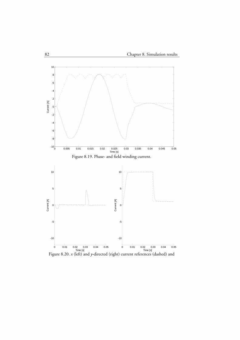
82 Chapter 8. Simulation results
0 0.005 0.01 0.015 0.02 0.025 0.03 0.035 0.04 0.045 0.05-10
-8
-6
-4
-2
0
2
4
6
8
10
Time [s]
Cur
rent
[A]
Figure 8.19. Phase- and field winding current.
0 0.01 0.02 0.03 0.04 0.05
-10
-5
0
5
10
Time [s]
Cur
rent
[A]
0 0.01 0.02 0.03 0.04 0.05
-10
-5
0
5
10
Time [s]
Cur
rent
[A]
Figure 8.20. x (left) and y-directed (right) current references (dashed) and

8.4. SMSM controlled by field voltage vector feed forward 83
actual currents.
0 0.01 0.02 0.03 0.04 0.050
2
4
6
8
10
12
14
16
18
20
Time [s]
Torq
ue [N
m]
0 0.01 0.02 0.03 0.04 0.05
40
42
44
46
48
50
Time [s]
Spee
d [ra
d/s]
Figure 8.21. Generated mechanical torque (left) and rotor rotational speed.

84 Chapter 8. Simulation results
0 0.005 0.01 0.015 0.02 0.025 0.03 0.035 0.04 0.045 0.05
-80
-60
-40
-20
0
20
40
60
80
100
Time [s]
Volta
ge [V
] and
Cur
rent
[A]
Figure 8.22. Field winding voltage (dot) and current (solid).
0 0.005 0.01 0.015 0.02 0.025 0.03 0.035 0.04 0.045 0.05
-100
-50
0
50
100
Time [s]
Volta
ge [V
] and
cur
rent
[A]
Figure 8.23. Applied phase voltage (dot) and phase current .

8.5. Torque compensation 85
-200 0 200-300
-200
-100
0
100
200
300Applied voltage vector
Voltage [v], x-direction
Volta
ge [v
], y-
dire
ctio
n
-200 0 200-300
-200
-100
0
100
200
300Voltage vector across field winding
Voltage [v], x-directionVo
ltage
[v],
y-di
rect
ion
-200 0 200-300
-200
-100
0
100
200
300Voltage vector across stator winding
Voltage [v], x-direction
Volta
ge [v
], y-
dire
ctio
n
Figure 8.24. Separated voltage vector.
Figure 8.19 shows that this type of controller produces the most pure sinusoidal phase currents.
Figure 8.20 reveals that this type of controller is the most suitable controller, out of those that are evaluated in these simulations. It is obvious that the transient behaviour is still a problem since the DC voltage source is limited. This may be alleviated by filtering the current reference signals.
Figure 8.22 show that the field winding requires higher voltage than in the other cases when using this type of controller.
In Figure 8.24 it is seen that the field voltage vector is similar to the other cases but the voltage across the stator is tweaked even more for reaching sinusoidal currents.
8.5 Torque compensation
The torque compensation method is an approach to force the SMSM to produce a more smooth torque. As mentioned earlier, this method holds the x-direction current reference to zero and modifies the y-direction current, taking the field winding current into account, so that the produced torque should be constant. The current controllers that are used are the standard PI controllers with the field voltage vector feed forward. The main results of interest are shown in Figure 8.25 to Figure 8.27.

86 Chapter 8. Simulation results
0 0.005 0.01 0.015 0.02 0.025 0.03 0.035 0.04 0.045 0.05-8
-6
-4
-2
0
2
4
6
8
Time [s]
Cur
rent
[A]
Figure 8.25. Phase- (solid) and field winding current.
0 0.01 0.02 0.03 0.04 0.05
-10
-5
0
5
10
Time [s]
Cur
rent
[A]
0 0.01 0.02 0.03 0.04 0.05
-10
-5
0
5
10
Time [s]
Cur
rent
[A]
Figure 8.26. x (left) and y-directed (right) current references (dashed) and actual currents (solid).

8.5. Torque compensation 87
0 0.01 0.02 0.03 0.04 0.050
2
4
6
8
10
12
14
16
18
20
Time [s]
Torq
ue [N
m]
0 0.01 0.02 0.03 0.04 0.05
40
41
42
43
44
45
46
47
48
49
50
Time [s]
Spee
d [ra
d/s]
Figure 8.27. Generated mechanical torque (left) and rotor rotational speed.
In Figure 8.25 it is shown that the phase current no longer has a sinusoidal behaviour. Instead of pure sinusoidal, the phase current shape is almost piecewise linear and piecewise sinusoidal.
The y-direction current reference in Figure 8.26 actually follows the inverse of the field winding current ripple at each point of time so that the product of these, and hence the torque, is constant.
The produced torque is, as expected, fairly constant and is shown in Figure 8.27.


Chapter 9 Laboratory results
9.1 Laboratory equipment
The laboratory measurements are performed in the IEA department lab at Lund University. The setup consists of two shaft-connected electric machines, one DC-machine and one SMSM. The DC-machine is controlled by two cascade interacting controllers, one current and one speed controller. The speed controlled DC-machine is fed from a four-quadrant power electronic converter and the SMSM is fed from a three-phase power electronic converter. The DC-machine and the SMSM are both connected to the same DC-link voltage. An overview of the laboratory setup can be seen in Figure 9.1.
The controllers for the two machines are implemented in the dSpace (version ds1104) environment. The dSpace environment offers the possibility to implement the controllers in the Matlab Simulink environment. The development procedure begins with simulation where the user can implement his controllers in the Simulink simulation environment. When the user is satisfied with the simulated controller performance, the implemented control software is compiled and downloaded to an external electronic board that executes the control software in real-time. The external board is then able to control the power electronic converters, perform analogue to digital and digital to analogue conversions of different signals and forward (and receive) information to the personal computer to be interpreted by the user.
Since vector control with sampling frequency of 10 kHz is a demanding task, the controllers are not implemented in the Simulink environment. The compiler that compiles the code to be downloaded to the external dSpace board is not efficient enough. The ratio of the sizes (number of code lines) between the compiled code and the handwritten code was approximately 20:1. Hand-written c-code thus made a great improvement in execution

90 Chapter 9. Laboratory results
time. Since the hardware of the dSpace board is limited, as an example, changing time between different multiplexed analogue to digital converters, and the fact that the user has no control of these limitations when generating code from the Simulink environment, the user is more aware of what is really happening in the processor unit when writing c-code. In the end it became also obvious that the dSpace user interface did not manage to show the correct timescale in the user interface, thus all the output signals had to be digital to analogue converted and then measured using an external oscilloscope on the external dSpace board signal output.
Figure 9.1. Laboratory setup sketch.
9.2 Measurements
Since the derived dedicated controller is very complex, experiments are performed when controlling the SMSM with standard PI controllers in the rotating reference frame. For implementing the dedicated controller, more computational resources are required than available with the ds1104 dSpace board. The SMSM is controlled with standard PI controllers and this is sufficient for comparison and evaluation of the simulation model.
The torque compensation method is implemented. Unfortunately, the mechanical torque transducers, available in the lab, have strongly limited dynamic properties that prevent the analysis of the torque dynamics that is necessary for evaluation of the torque compensation method. Another fact
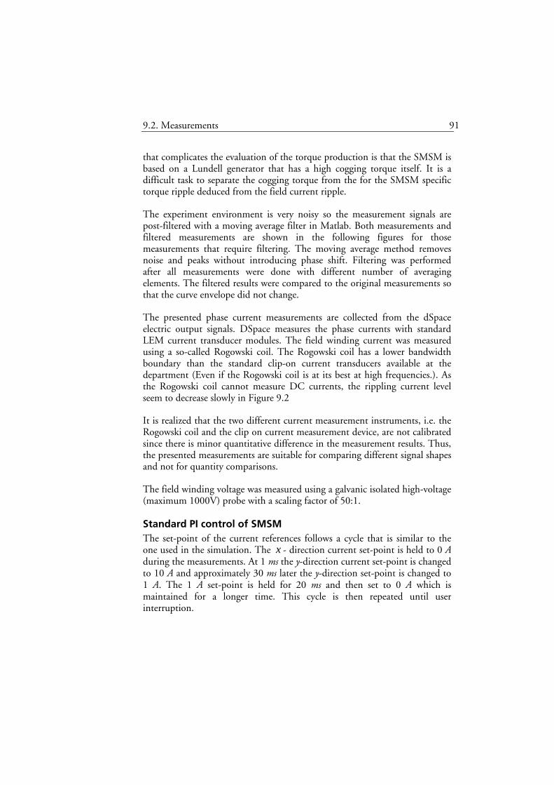
9.2. Measurements 91
that complicates the evaluation of the torque production is that the SMSM is based on a Lundell generator that has a high cogging torque itself. It is a difficult task to separate the cogging torque from the for the SMSM specific torque ripple deduced from the field current ripple.
The experiment environment is very noisy so the measurement signals are post-filtered with a moving average filter in Matlab. Both measurements and filtered measurements are shown in the following figures for those measurements that require filtering. The moving average method removes noise and peaks without introducing phase shift. Filtering was performed after all measurements were done with different number of averaging elements. The filtered results were compared to the original measurements so that the curve envelope did not change.
The presented phase current measurements are collected from the dSpace electric output signals. DSpace measures the phase currents with standard LEM current transducer modules. The field winding current was measured using a so-called Rogowski coil. The Rogowski coil has a lower bandwidth boundary than the standard clip-on current transducers available at the department (Even if the Rogowski coil is at its best at high frequencies.). As the Rogowski coil cannot measure DC currents, the rippling current level seem to decrease slowly in Figure 9.2
It is realized that the two different current measurement instruments, i.e. the Rogowski coil and the clip on current measurement device, are not calibrated since there is minor quantitative difference in the measurement results. Thus, the presented measurements are suitable for comparing different signal shapes and not for quantity comparisons.
The field winding voltage was measured using a galvanic isolated high-voltage (maximum 1000V) probe with a scaling factor of 50:1.
Standard PI control of SMSM The set-point of the current references follows a cycle that is similar to the one used in the simulation. The x - direction current set-point is held to 0 A during the measurements. At 1 ms the y-direction current set-point is changed to 10 A and approximately 30 ms later the y-direction set-point is changed to 1 A. The 1 A set-point is held for 20 ms and then set to 0 A which is maintained for a longer time. This cycle is then repeated until user interruption.

92 Chapter 9. Laboratory results
Phase and field current measurements are shown in Figure 9.2. As shown, the field winding current does not fall as fast as in the simulation. This difference is discussed in Chapter 10.
0 0.01 0.02 0.03 0.04 0.05-10
-8
-6
-4
-2
0
2
4
6
8
10
Time [s]
Cur
rent
[A]
0 0.01 0.02 0.03 0.04 0.05-10
-8
-6
-4
-2
0
2
4
6
8
10
Time [s]
Cur
rent
[A]
Figure 9.2. Phase- (blue) and field (red) current. (filtered signals on the right)
In Figure 9.3 the x- and y-direction current set-points and actual currents are shown. Red line is actual value of the current and blue line is current set-point. In the x-direction that is shown in the two plots on the left, the current set-point is held to zero. The rise-time of the current is measured to approximately 3 ms that is shorter than the simulations indicated in Figure 8.6 (5 ms) but still in the same order. It is also verified that there is a cross-connection between the x - and y-direction.

9.2. Measurements 93
0 0.01 0.02 0.03 0.04 0.05-3
-2
-1
0
1
2
3
Time [s]
Cur
rent
[A]
0 0.01 0.02 0.03 0.04 0.05-3
-2
-1
0
1
2
3
Time [s]
Cur
rent
[A]
0 0.01 0.02 0.03 0.04 0.05-2
0
2
4
6
8
10
12
Time [s]
Cur
rent
[A]
0 0.01 0.02 0.03 0.04 0.05-2
0
2
4
6
8
10
12
Time [s]
Cur
rent
[A]
Figure 9.3. x- (left) and y-direction (right) current (red) and current set-points (blue). Bottom two figures show the filtered signals and the two plots on the top shows the
unfiltered signals.
Figure 9.4 shows the voltage across (blue) and the current through (red) the field winding. It is evident that the shape of the voltage across the field winding differs between simulation and experimental results. This will be discussed in next chapter. As expected, there is a voltage ripple that can be referred to the current derivative as for all inductances.

94 Chapter 9. Laboratory results
0 0.005 0.01 0.015 0.02 0.025 0.03 0.035 0.04 0.045 0.05-10
0
10
20
30
40
50
60
70
Time [s]
Cur
rent
[A] (
red)
and
Vol
tage
(blu
e)
Figure 9.4. Field winding voltage (blue) and current (red).
Figure 9.5 to Figure 9.7 shows the same measurement results as the previous three plots but with the torque compensation method implemented. There is a constant torque set-point that further generates a varying y-direction current set-point depending on the field winding current.
The phase current shape in Figure 9.5 agrees well with the simulation results. The same decaying behavior of the field winding current is present with and without the torque compensation behavior. It is also traceable that the field current ripple is less utilizing the torque compensation method.

9.2. Measurements 95
0 0.01 0.02 0.03 0.04 0.05-10
-8
-6
-4
-2
0
2
4
6
8
10
Time [s]
Cur
rent
[A]
0 0.01 0.02 0.03 0.04 0.05-10
-8
-6
-4
-2
0
2
4
6
8
10
Time [s]
Cur
rent
[A]
Figure 9.5. Phase- (blue) and field current. (filtered signals on the right)
In Figure 9.6 it is also shown that the current controllers fulfill the task to follow the varying y-direction current reference for generating a more constant torque. From this figure, it is also evident that there is an upper boundary in the rotational speed for which the torque compensation method is applicable. The current stiffness and DC-link voltage together with the performance of the current controllers determine the dynamics of the current controller. This fact does not introduce any trouble since the vehicle mass itself act like a low pass filter for the interacting forces. (i.e. driving and braking torques). A cross-coupling between the x- and y-direction is still present.

96 Chapter 9. Laboratory results
0 0.01 0.02 0.03 0.04 0.05-3
-2
-1
0
1
2
3
Time [s]
Cur
rent
[A]
0 0.01 0.02 0.03 0.04 0.05-3
-2
-1
0
1
2
3
Time [s]
Cur
rent
[A]
0 0.01 0.02 0.03 0.04 0.05-2
0
2
4
6
8
10
12
Time [s]C
urre
nt [A
]
0 0.01 0.02 0.03 0.04 0.05-2
0
2
4
6
8
10
12
Time [s]
Cur
rent
[A]
Figure 9.6. x- (left) and y-direction (right) current (red) and current setpoints (blue). Bottom two figures show the filtered signals and the two plots on the top shows the
unfiltered signals.
In Figure 9.7 the voltage across the field winding and the current through it is shown when utilizing the torque compensation method. Since the field winding current ripple is less according to previous reasoning, also the voltage ripple across the field winding is less.
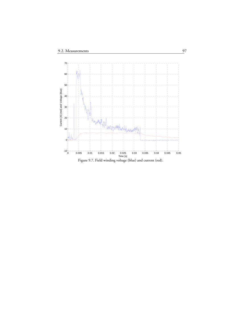
9.2. Measurements 97
0 0.005 0.01 0.015 0.02 0.025 0.03 0.035 0.04 0.045 0.05-10
0
10
20
30
40
50
60
70
Time [s]
Cur
rent
[A] (
red)
and
Vol
tage
(blu
e)
Figure 9.7. Field winding voltage (blue) and current (red).


Chapter 10 Deviations between simulation and laboratory results
This chapter discusses some ideas of why some simulation results deviate from laboratory results.
There is an error of basic character that can be perceived when studying the SMSM circuit at page 49. The consequences can be seen in Figure 9.2 and Figure 9.5 where the field winding current is declining with “its own pace” and is not influenced by the phase currents. Studying the SMSM electric circuit again one realizes that the minimum voltage across the field winding is
dU⋅−2 were dU is the forward voltage drop across one diode in the diode bridge rectifier. Thus, the diode bridge rectifier clamps the negative voltage transients across the field winding to dU⋅−2 V. When all the phase currents are lower than the field winding current, the stored magnetic energy (in the field winding) tries to maintain the flux level and generates a negative voltage that is clamped by the diode bridge rectifier. A closer examination of Figure 9.4 and Figure 9.7 reveals that there actually is a low negative voltage across the field winding when this occurs.
The diminishing of the field winding current can be estimated by solving the differential equation for the roughly estimated demagnetizing circuit shown in Figure 10.1. The voltage source corresponds to the voltage drop across the diode bridge rectifier, the resistance and inductance (self inductance) are the field winding resistance and inductance respectively. As an initial condition for the differential equation, the field winding current equals the field winding current present at the moment just before the decrement of the phase currents.

100 Chapter 10. Deviations between simulation and laboratory results
Figure 10.1. Equivalent demagnetization circuit.
The differential equation for the equivalent demagnetization circuit is shown in Equation 33 and its solution in Equation 34.
02 =⋅−⋅−⋅− d
u
ff
u
ff UiR
dtdi
L
Rf
32143421
Equation 33. Differential equation for the demagnetization circuit.
tLR
f
df
f
df
f
f
eRU
tiRU
ti⋅−
⋅⎟⎟⎠
⎞⎜⎜⎝
⎛ ⋅+=+
⋅−=
2)0(
2)(
Equation 34. Current in the equivalent demagnetization circuit.
With Rf=0.65 Ω, Lf=70 mH and Ud=0.9 V the demagnetization curve shown in Figure 10.2 (blue) is achieved. Since the voltage source in is a model of the diode bridge, it is obvious that it is not able to drive a current in the negative direction since it cannot deliver any energy.

101
0 0.02 0.04 0.06 0.08 0.1 0.12 0.14 0.16 0.18 0.2-1
0
1
2
3
4
5
6
7
8
9
Time [s]
Cur
rent
[A] (
red)
and
Vol
tage
(blu
e)
Figure 10.2. Demagnetization curve for the equivalent circuit, measured (red) and calculated (blue).
In Figure 10.2 the theoretical demagnetization curve and the measured field winding current are plotted for comparison. Of course, there are uncertainties in parameter estimations that may be of importance for obtaining similar shapes of the field current. After approximately 35 ms, the current set-point changes to a lower value and from there on, the field winding current decreases while the stored magnetic energy is discharged in the field winding resistance and freewheeling diodes.
For studying the diode bridge rectifier behaviour, further simulations are performed in a simulation environment for electronic simulations. The used software, LTspice, is free of charge and supplied by the electronics manufacturer Linear Technology at their internet webpage (www.linear.com). The software is flexible and easy to use. In the electronics simulation the magnetic connection between the stator and the rotor is not taken into account but since the circuit is fed from ideal current sources and for understanding the operation of the diode bridge rectifier in this application,

102 Chapter 10. Deviations between simulation and laboratory results
the circuit fulfil the task.
The circuit used for electronic simulation is shown in Figure 10.3.
Figure 10.3. The SMSM electric circuit for simulation.
The shape of the three phase currents produced by the 8 current sources (on the left) and applied to the SMSM circuit are shown in Figure 10.4 together with the consequent field winding current. The current cycle in this simulation begins with three sinusoidals with the amplitude 10 A and frequency similar to previous frequencies occurring in previous simulations (38 Hz). At approximately 50 ms the amplitudes are changed to 1A as in previous simulations. In the LTspice simulation results, the field winding current fall-time, from 10 A to 0 A, is approximately 165 ms. This result corresponds to the results from Equation 34 very well.
In Figure 10.5 currents involving one phase in the circuit during the freewheeling period are shown. This figure gives an understanding of how the rectifying circuit works in this application. First, from Figure 10.5 it is clear that the upper diodes conduct when the particular phase current is positive and the lower diodes conduct when the particular current is negative. The

103
freewheeling field current is shared between the three phases in the rectifier and forms the envelope of the current through the diode currents. The phase current is equally shared and lowers the current in the lower diode at the same time as it raises the current in the upper diode.
Since all diodes are conducting in the freewheeling region, ideally assuming no forward voltage drop, the three phases in the electric machine are connected in a common star configuration.
0 0.05 0.1 0.15 0.2-10
-8
-6
-4
-2
0
2
4
6
8
10
Time [s]
Cur
rent
[A]
Figure 10.4. Applied phase currents and consequent field current.

104 Chapter 10. Deviations between simulation and laboratory results
0 0.05 0.1 0.15 0.2
-8
-6
-4
-2
0
2
4
6
8
10
Time [s]
Cur
rent
[A]
iL1iD1iD2iL4/3
Figure 10.5. Phase current (black) compared to diode bridge rectifier currents (blue and red) and field winding current divided by three.
10.1 Consequences of the deviations
As seen in previous section, magnetizing of the field winding in a SMSM is much faster than demagnetization. The consequences of this are not considered critical for the BAS application since the acceleration of an ICE is assumed slower than the demagnetization of a SMSM.

Chapter 11 Conclusions
The Series Magnetized Synchronous Machine is an electrically magnetized synchronous machine with a novel field winding circuit configuration.
The SMSM is considered in an automotive application implementing Stop&Go functionality as well as an assisting source of torque in the weak region (low rotational speeds) of the ICE.
Since the phase currents in an SMSM are forced to pass through two diodes and two sliprings there are voltage drops in the circuit. Low voltage, high current applications may result in a low efficiency of the electric drive. In applications where the voltage drop across the sliprings and the diodes only correspond to a fraction (few percents) of the DC-link voltage (In a system with well matched voltage levels between machine and DC-link voltage) the SMSM is a competitive alternative.
Simulations are performed on a vehicle basis for minimization of the fuel consumption. As the electric machine (synchronous machine) performs best in its nominal operating region, minimum fuel consumption is found for a certain electric machine size. The optimum electric machine rated power is approximately 5 kW, nominal power, which is a rather small machine but sufficient for implementing Stop&Go functionality and torque assist at low rotational speeds. Since 5 kW machine output covers the peaks of the demands on the electric drive, the power rating of the converter should be similar. The machine is assumed to be a multi-pole electric machine for being capable of producing the high torque that is demanded. Yet, the number of poles is limited by e.g. the computational capability of the controlling DSP.
In this thesis, a simulation model for the SMSM is provided. The simulation model is well working, i.e. provides a high degree of agreement compared with measurement results, for steady state operation and positive current
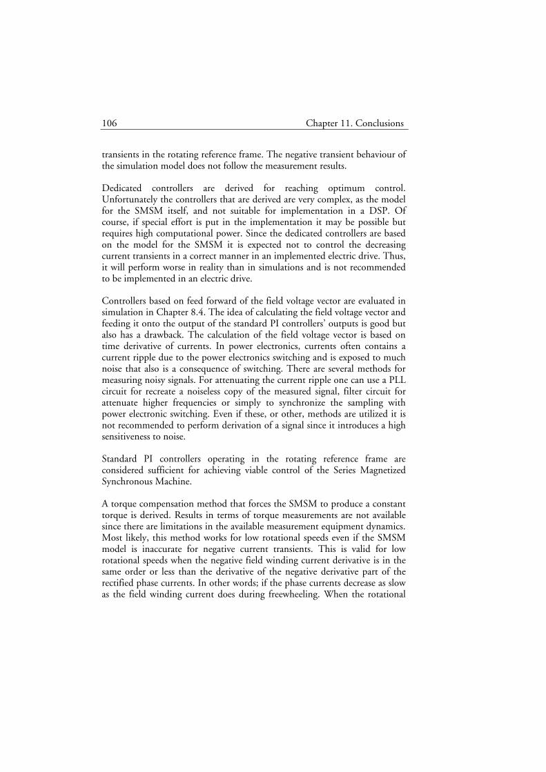
106 Chapter 11. Conclusions
transients in the rotating reference frame. The negative transient behaviour of the simulation model does not follow the measurement results.
Dedicated controllers are derived for reaching optimum control. Unfortunately the controllers that are derived are very complex, as the model for the SMSM itself, and not suitable for implementation in a DSP. Of course, if special effort is put in the implementation it may be possible but requires high computational power. Since the dedicated controllers are based on the model for the SMSM it is expected not to control the decreasing current transients in a correct manner in an implemented electric drive. Thus, it will perform worse in reality than in simulations and is not recommended to be implemented in an electric drive.
Controllers based on feed forward of the field voltage vector are evaluated in simulation in Chapter 8.4. The idea of calculating the field voltage vector and feeding it onto the output of the standard PI controllers’ outputs is good but also has a drawback. The calculation of the field voltage vector is based on time derivative of currents. In power electronics, currents often contains a current ripple due to the power electronics switching and is exposed to much noise that also is a consequence of switching. There are several methods for measuring noisy signals. For attenuating the current ripple one can use a PLL circuit for recreate a noiseless copy of the measured signal, filter circuit for attenuate higher frequencies or simply to synchronize the sampling with power electronic switching. Even if these, or other, methods are utilized it is not recommended to perform derivation of a signal since it introduces a high sensitiveness to noise.
Standard PI controllers operating in the rotating reference frame are considered sufficient for achieving viable control of the Series Magnetized Synchronous Machine.
A torque compensation method that forces the SMSM to produce a constant torque is derived. Results in terms of torque measurements are not available since there are limitations in the available measurement equipment dynamics. Most likely, this method works for low rotational speeds even if the SMSM model is inaccurate for negative current transients. This is valid for low rotational speeds when the negative field winding current derivative is in the same order or less than the derivative of the negative derivative part of the rectified phase currents. In other words; if the phase currents decrease as slow as the field winding current does during freewheeling. When the rotational

107
speed increases, the field winding current ripple decreases so there is no longer any need for torque compensation. The conclusion from this thus is that a SMSM generates a constant torque for higher rotational speeds. It must also be mentioned that the time constant of the field winding circuit in a SMSM is the same as for an EMSM but since the field winding is magnetically demagnetized in two series connected diodes, the demagnetization time is half as long as in the EMSM case that is fed from a step down converter.


Chapter 12 Future work
The implementation of the SMSM drive in a BAS application need more work. A well working controller is implemented in a DSP by programming in the C-language. Since it is shown in this thesis that a standard PMSM-like vector control is enough, implementation of an on-board control system needs no research. An on-board three phase inverter need to be designed to fulfil the requirements such as e.g. size, weight, cooling, operating ambient temperature, overload and integration. The control system also requires communication with other on-board computers for protection systems, input and output signals.
It would have been interesting to quantify the effects of the torque compensation method, refining the simulation model so that it is valid also for negative current transients and for the field voltage vector estimation. If the field voltage vector is known, it is of course also very interesting to implement the field voltage vector control strategy as an alternative to the very complicated dedicated controllers.


Bibliography
Articles Campbell R.J., Rajashekara K., Evaluation of Power Devices for Automotive Hybrid and 42V Based Systems, 2004 SAE World Congress, March 2004.
Jonasson K. (2002). Analysing Hybrid Drive System Topologies, Licentiate thesis, Department of Industrial Electrical Engineering and Automation, Lund University, Sweden. Jourdan L., Schanen JL., Roudet J., Bensaied M., Segueni K (2002). Design Methodology for Non Insulated DC-DC converter: Application to 42V-14V “PowerNet”, IEEE Power Electronics Specialists Conference, Pesc ’02, Volume 4, 23-27 June 2002 Page(s):1679 – 1684 Mudannayake C.P., Rahman M.F., An integrated starter alternator for the 42V PowerNet, Power Electronics and Drive Systems, 2003, PEDS 2003, Volume 1, 17-20 Nov. 2003 Page(s):648 - 653 Vol.1
Nicastri P.R, Huang H., Jump starting 42V PowerNet vehicles, IEEE Aerospace and Electronic Systems Magazine, Voume 15, Issue 8, Aug. 2000, Page(s): 25-31 Reiter F.B. Jr, Rajashekara K., Krefta R.J., Salient Pole Generators for Belt-Driven Automotive Alternator Applications, IEEE Industry Applications Conference, 2001, Conf. Rec., Volume 1, 30 Sept.-4 Oct. 2001 Page(s):437 - 442 vol.1

112 Chapter 11. Conclusions
Shafer, G.A, FMC High power density electric drive technology, WESCON Conference Record, 1994, Pages 172 - 175
Shaotang C., Lequesne B., Henry R.R., Yanhong X, Ronning J.J., Design and testing of a Belt-Driven Induction Starter-Generator, IEEE International Electric Machines and Drives Conference, 2001, Page(s):252 – 260 Wilson T. G., The Evolution of Power Electronics, IEEE Transaction on Power Electronics, Vol 15, No 3, May 2000
Books Alaküla M., Power Electronic Control, Course literature from Department of Industrial Electrical Engineering and Automation, Lund University, Sweden (2002) Bengtsson H.-U., Konsten att uppskatta omvärlden, ISBN:91-534-1922-7, Ica Bokförlag, Sweden (1998) Internet http://www.dieselnet.com/ (2006-08-28), Online information service on clean diesel engines and diesel emissions Reports European Commission – Office for official Publications of the European Communities, European Energy and Transport Trends to 2030, ISBN: 92-894-4444-4 (2003)
Theses

113
Hagstedt D., Analysis of a Series magnetized Lundell alternator, MSc Thesis, Dept. of Industrial Electrical Engineering and Automation. Lund University, Sweden (2004), Marksell S., EMC Aspects of PWM Controlled Loads in Vehicles., Licentiate Thesis, Dept. of Industrial Electrical Engineering and Automation, Lund University, Sweden. (2004)
Tonin D., A novel synchronous drive using series magnetized synchronous machine with a special position sensing., MSc Thesis, Dept. of Industrial Electrical Engineering and Automation, Lund University, Sweden. (2003)


Appendix A
A.1 Abbreviations
Abbreviation Explanation BAS Belt driven Alternator and Starter BLDC Brushless Direct Current machine DC Direct Current DFIG Doubly Fed Induction Generator DSP Digital Signal Processor EHR Electric Hybridization Rate EMC ElectroMagnetic Compatibility EMDC Electrically Magnetized Direct Current Machine EMF ElectroMotive Force EMI ElectroMagnetic Interfearance EMSM Electrically Magnetized Synchronous Machine HEV Hybrid Electric Vehicle ICE Internal Combustion Engine IGBT Insulated Gate Bipolar Transistor IM Induction machine MHEV Mild Hybrid Electric Vehicle MOSFET Metal Oxide Semiconductor Field Effect Transistor PMDC Permanently Magnetized Direct Current Machine PMSM Permanently Magnetized Synchrnous Machine SEK Currency of Sweden, Swedish crowns Si Silicon SiC Silicon Carbide SMSM Series Magnetized Synchronous Machine SRM Switched Reluctance Machine