~~

NASA CONTRACTOR REPORT 177488

Contraction Design for Small Low-Speed Wind Tunnels *

.

J. H . Bell R. D. Mehta

- (kASA-CB- 177488) C G I I R A C T I C L CES161 FOB 189-13753 SEALL LOU-SEEED h l B D I G L Y E L S (Stanford

n n i r . ) 39 F CSCL 20D Unclas

G3/34 017F8C2

,

CONTRACT NASZ- NCC-2-294 August 1988

~ ~- ~

. < , ,

NASA CONTRACTOR REPORT 177488

Contraction Design f o r Small Low-Speed blind Tunnels

J. H. Bell R. D. Mehta Stanford University Stanford, California

Prepared by Ames Research Center under Cooperative Agreement NCC-2-294 August 1988

National Aeronautics and Space Administration

ABSTRACT

An iterative design procedure has been developed for tw+ or three-dimensional con- tractions installed on small, low-speed wind tunnels. The procedure consists of first com- puting the potential flow field and hence the pressure distributions along the walls of a contraction of given size and shape using a three-dimensional numerical panel method. The pressure or velocity distributions are then fed into two-dimensional boundary layer codes to predict the behavior of the boundary layers along the walls. For small, low-speed contractions it is shown that the assumption of a laminar boundary layer originating from stagnation conditions at the contraction entry and remaining laminar throughout passage through the "successful" designs is justified. This hypothesis was confirmed by comparing the predicted boundary layer data at the contraction exit with measured data in existing wind tunnels. The measured boundary layer momentum thicknesses at the exit of four existing contractions, two of which were 3-D, were found to lie within 10% of the predicted values, with the predicted values generally lower. From the contraction wall shapes inves- tigated. the one based on a fifth-order polynomial was selected for installation on a newly designed mixing layer wind tunnel.

1

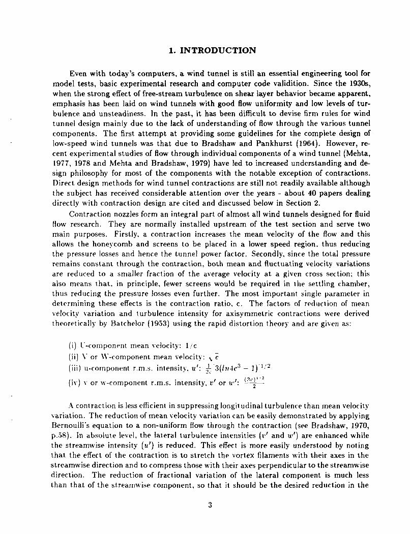
NOMENCLATURE

C:

C, : H e : H , : L: P: Re: R: u,v,w: u, : U J , u J , u+:

u,v,w:

Contract ion rat io Pressure coefficient on contraction wall Contraction height at exit Contraction height at inlet Contract ion length Static pressure on contraction wall Reynolds number, U L/u Contraction radius of curvature Mean velocity in the X,Y,Z directions, respectively Free-stream velocity in the wind tunnel test section Fluctuating velocity components in the X,Y,Z direct ions, respectively Instantaneous velocity in the X,Y,Z directions, respectively, e.g. u = U + ut Cartesian coordinates for streamwise, normal, Non-d irnension al s treamw ise distance, X/ L and spanwise directions, respectively.

Kinematic viscosity Density Contraction match point

_ _ (over bar) Time-averaged quantity 0 r n , I I : Maximum value at station

2

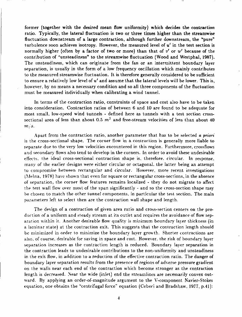
1. INTRODUCTION

Even with today's computers, a wind tunnel is still an essential engineering tool for model tests, basic experimental research and computer code validition. Since the 193Os, when the strong effect of free-stream turbulence on shear layer behavior became apparent, emphasis has been laid on wind tunnels with good flow uniformity and low levels of tur- bulence and unsteadiness. In the past, it has been difficult to devise firm rules for wind tunnel design mainly due to the lack of understanding of flow through the various tunnel components. The first attempt a t providing some guidelines for the complete design of low-speed wind tunnels was that due to Bradshaw and Pankhurst (1964). However, re- cent experimental studies of flow through individual components of a wind tunnel (Mehta, 1977, 1978 and Mehta and Bradshaw, 1979) have led to increased understanding and de- sign philosophy for most of the components with the notable exception of contractions. Direct design methods for wind tunnel contractions are still not readily available although t h e subject has received considerable attention over the years - about 40 papers dealing directly with contraction design are cited and discussed below in Section 2.

Contraction nozzles form an integral part of almost all wind tunnels designed for fluid flow research. They are normally installed upstream of the test section and serve two main purposes. Firstly. a contraction increases the mean velocity of the flow and this allows the honeycomb and screens to be placed in a lower speed region. thus reducing the pressure losses and hence the tunnel power factor. Secondly, since the total pressure remains constant through the contraction. both mean and fluctuating velocity variations are reduced to a smaller fraction of the average velocity at a given cross section: th i s also means t h a t . in principle, fewer screens would be required in the settling chamber, thus reducing the pressure losses even further. The most important single parameter in determining these effects is the contraction ratio, c. The factors of reduction of mean velocity variation and turbulence intensity for axisymrnetric contractions were derived theoretically by Batchelor (1953) using the rapid distortion theory and are given as:

( i ) L-component mean velocity: 1 ' c ( i i ) 1- or \\'-component mean velocity: ( i i i ) u-cornporient r.m.s. intensit!. u t : 1 - c 3(!?t4c3 - I)","

(?.C)''2 ( iv) v or lr-component r.m.s. intensity. d or w': -__

- c

2

-4 contraction is less efiicient in suppressing lorigit udinai turbulence t h a n mean velocity variation. The reduction of mean velocity variation can be easily demonstrated by applying Bernoulli's equation to a non-uniform flow through the contraction (see Bradshaw, 1970, p.38). In absolute level, the lateral turbulence intensities (19' and u,') are enhanced while the streamwise intensity (u') is reduced. This effect is more easily understood by noting that the effect of the contraction is to stretch the vortex filaments with their axes in the streamwise direction and to compress those with their axes perpendicular to the streamwise direction. The reduction of fractional variation of the lateral component is much less than that of the stream\rise component, so that it should be the desired reduction in the

9 J

former (together with the desired mean flow uniformity) which decides the contraction ratio. Typically, the lateral fluctuation is two or three times higher than the streamwise fluctuation downstream of a large contraction, although further downstream, the Upuren turbulence soon achieves isotropy. However, the measured level of u‘ in the test section is normally higher (often by a factor of two or more) than that of v‘ or w’ because of the contribution of “unsteadiness” to the streamwise fluctuation (Wood and Westphal, 1987). The unsteadiness, which can originate from the fan or an intermittent boundary layer separation, is usually in the form of a low frequency oscillation which mainly contributes to the measured streamwise fluctuation. It is therefore generally considered to be sufficient to ensure a relatively low level of u’ and assume that the lateral levels will be lower. This is, however, by no means a necessary condition and so all three components of the fluctuation must be measured individually when calibrating a wind tunnel.

In terms of the contraction ratio, constraints of space and cost also have to be taken into consideration. Contraction ratios of between 6 and 10 are found to be adequate for most small, low-speed wind tunnels - defined here as tunnels with a test section cross- sectional area of less than about 0.5 m2 and free-stream velocities of less than about 40 mi's.

Apart from the contraction ratio, another parameter that has to be selected a priori is t h e cross-sectional shape. The corner flow in a contraction is generally more liable to separate due to the very low velocities encount>ered in this region. Furthermore, crossflows and secondary flows also tend to develop in the corners. In order to avoid these undesirable effects. the ideal cross-sectional contraction shape is. therefore. circular. In response. many of t h e earlier designs were either circular or octagonal. the latter being an attempt to compromise between rectangular and circular. However. more recent investigations (l lehta, 1978) have shown that even for square or rectangular cross-sections, in the absence of separation. the corner flow features remains localized - they do not migrate to affect the test wall flow over most of the span significantly - and so the cross-section shape may be chosen to match the other tunnel components. in particular the test section. The main parameters left to select then are the contraction wall shape and length.

The design of a contraction of given area ratio and cross-section centers on the p r e duct ion of a uniform and steady stream a t its outlet and requires the avoidance of flow sep- arat ion ivithin it. Another desirable flow quality is minimum boundary laj,er thickness (in a laminar state) at the contraction exit. This suggests that the contraction length should bc niinirnized in order to minimize the boundary layer growth. Shorter contractions are also. of course. desirable for saving in space and cost. However. t h e risk of boundary layer separation increases as the contraction length is reduced. Boundary layer separation in t h e contraction leads to undesirable contributions to the non-uniformity and unsteadiness in the exit flow, in addition to a reduction of the effective contraction ratio. The danger of boundary layer separation results from the presence of regions of adverse pressure gradient on the walls near each end of the contraction which become stronger as the contraction length is decreased. Near the wide (inlet) end the streamlines are necessarily convex out- ward. By applying an order-of-magnitude argument to the V-component Navier-Stokes equation, one obtains the “centrifugal force“ equation (Cebeci and Bradshaw. 1977. p.4 1):

where R is the radius of curvature of the surface or strictly the considered streamline. So the static pressure near the walls is greater than that near the centerline and, therefore, greater than the average pressure over the cross-section. Thus the wail pressure increases from a point far upstream to a point in the wide end, before decreasing as the effect just described is overwhelmed by the effects of decreasing cross-sectional area. The converse applies a t the narrow end. However, in general, the boundary layer is less liable to sepa- rate a t the contraction exit, due to its increased skin friction coefficient caused by passage through the strong favorable pressure gradient. Also, the concave curvature at the con- traction inlet has a destabilizing effect on the boundary layer, in contrast to the convex curvature near the outlet which has a stabilizing effect (Bradshaw, 1973).

It is normally possible to avoid separation by increasing the contraction length suffi- ciently, provided it has a reasonable wall shape so that the boundary layer does not grow excessively near the exit. Increasing the length, however, results in increased boundary layer growth due to skin friction, not to mention the space/cost consideration. On the other hand, a contraction that is too short also suffers from some disadvantages. in addition to the boundary layer separation problem discussed above. For example, when a contraction is shortened. say by 3 L . the upstream and downstream distances within which local veloc- i ty profile distortions (due to streamline curvature effects) are still relatively high increase. nnd the effective saving is less t h a n AL. The decay of velocity nonuniformity in the test section can be estimated by solving the Laplace equation for a semi-infinite straight duct n i t h arbitrary inlet velocity profile (Morel, 1976). The first term of the solution series. Mhich will predominate for large distance from the inlet plane. shows that the nonuni- formity decays as e r y ( - 2 z r ( H e ) . Thus t h e velocity nonuniformity decays to 10% of its original value by a distance of 0.371-1, downstream of the contraction exit.

A design satisfying all criteria will be such that separation is just avoided (implying a minimum acceptable length) and the exit non-uniformiq is equal to the maximum tolerable level for a given application (typically less than 1% variation outside the boundary layers).

Before entering the proposed design scheme. a review of some of the past work is first presented in Section 2. The present computational approach is described in Section 3 and t h e results of the proposed method and design procedure are presented and discussed in Section 4 . Thc concluding remarks are given in Section 5 .

2. LITERATURE REVIEW

Although we have attempted to make this review exhaustive, considering the number of papers published on the subject, it is quite possible that some references have been overlooked.

In the absence of separation, the flow in a contraction is adequately described by the Laplace equation. The solution of this linear equation is relatively easy for simple geome

5

tries (especially in the case of axisymmetric or two-dimensional flows) and hence many solutions have been derived over the years. In both, axisymmetric and two-dimensional cases, the standard technique for contraction design was to define a centerline velocity distribution and then calculate a set of stream surfaces from it. Any stream surface (or a pair of surfaces in the 3-D case) could then be chosen as the wall. Most analyses of axisymmetric contractions are based on a series solution of either the Laplace equation for the velocity potential (Tsien, 1943, Szczeniowski, 1943, Thwaites, 1946 and Bloomer, 1956). or the Stokes-Beltrami equation for the stream function (Cohen and Ritchie, 1962), for a given velocity distribution along the centerline. The solution produces an infinite set of stream-surfaces at different distances from the axis, and the most distant one with tolerable pressure gradient (leading to the shortest contraction) is chosen as the wall con- tour. Some years later, Bossel (1969) reformulated Thwaites’ solution which made the method faster and easier to use while Tulapurkara (1980) made an attempt at optimizing the number of terms in the solution.

Early researchers used a very strict definition of a “tolerable” pressure gradient. They sought stream surfaces with a monotonically increasing velocity, thus eliminating the pos- sibility of an unfavorable pressure gradient along the wall which might cause separation. This condition could only be fulfilled by a contraction of infinite length. which asymptoti- cally approached its upstream and downstream widths. Thus, t he question became one of choosing the points a t which to “cut” the contraction and then fairing into the upstream and downstream sections. Of course, the process of cutting produced a contraction with adkerse pressure gradients. but this was considered unavoidable. The logical criterion for such a contraction .‘length” was one related to the exit flow uniformity; Tsien (1943) and Smith and M‘ang (194 1) used esit flow uniformity considerations to decide where their contraction contours should be terminated. The Tsien design method was further gener- alized by Barger and Bomen (1972) w h o simplified the way in which the design velocity d is t rib II t ion was for niu 1 ated .

Lighthill (1945) and Cheers (1945) used a variation of th is popular technique by allow- ing for the problems related to finite length contractions from the start. They defined the velocit! distributions to be solved for such that some tolerable effects due to the adverse pressure gradients were already included. This made the blending of the chosen stream surface with the upstream and downstream sections much smoother. Coldstein (1945) was apparently the first to solbe the Laplace equation for a finite two-dimensional contraction. He found that t h e resulting contraction sections had very large adxerse pressure gradi- ents near the inlet and outlet. So the problem of adverse pressure gradients existing in contraction sections of finite length still remained.

These difficulties also prompted more work on the two-dimensional case in the hope tha t techniques only usable in this case would make the problem more tractable, and that the results would be applicable to three-dimensional contractions. Two-dimensional cases were usually solved in the hodograph (V, V) plane. -4s with other analytic techniques, a streamwise xelocity distribution is assumed and the corresponding wall shape is then cal- culated. The resulting contraction can either he infinite (Libby and Reiss, 1951) or finite (Gibbings and Dixon. 1957) depending o n the exact method used to calculate the wall shape and on the allowances made for the adverse pressure gradients (Gibhings, 1964).

6

Jordinson's (1961) hodograph method, for large contraction ratios, deserves special men- tion because he solved the flow in each end of the contraction separately, assuming that, in the limit of high contraction ratios, the shape of the wide end becomes independent of that of the narrow end (and vice versa) because the flow in between is closely radial without significant longitudinal streamline curvature. Jordinson found that this technique worked very well for c > 10. Other methods for two-dimensional contractions were also tried; most were modifications of techniques used on axisymmetric contractions (Swamy, 1961, 1962. Szczeniowski, 1963, and Mills, 1968).

Attempts to derive axisyrnmetric contraction shapes from two-dimensional ones have met with limited success. Since most contractions have relatively large contraction ratios, any simple scaling of cross-sectional area can lead to unacceptable wall shapes. An excep- tion is the approximate method of Whitehead et a]. (1951) for calculating the flow in an axisyrnmetric contraction once the flow in the two-dimensional contraction with the same wall shape is known. Although it is assumed that the streamline shapes are the same in both cases, the velocity along the streamlines in the axisymmetric case is made to satisfy the axisymmetric continuity equation.

The problem of defining an effective length for the infinite contractions produced by most analytic methods continued to be studied (Gibbings, 1964, 1966 and Lau 1964, 1966). Gibbings and Lau determined that the most conservative condition establishing the *'length" of a contraction was how rapidly the centerline velocity approached its asymptotic value at the exit. L-nder some cicumstances. however. velocity uniformity at the exit is a more stringent condition (Lau, 1966). Another approach to the problem was developed by Gay et al. (1973). who used a turbulent boundary layer model to predict the largest allowable adverse pressure gradient. and thus the shortest allonable stream surface, for their contraction.

With the onset of computers. numerical methods have been increasingly applied to contraction design. Smith and Pearce (1959) gave a numerical method for calculating the flow (either two-dimensional or axisymmetric) within a given boundary using a distribu- t ion of sources. illore recent Iv. Laine and Harjuniaki (1975) computed the potential flow in asis! rnrnetric contractions by a n accurate method in which the Stokes-Beltrami equation is solved with a finite difference approach. .An alternative approach used by Mikhail and Rainbird (19i8) is rerninixent of Jordinson's (1961) study. llikhail and Rainbird consid- ered the contraction shape as a matched set of inlet and exit regions. Inlet flow separation was assumed to be affected mainly by the inlet region shape. with exit flow nonuniformity influcnced mostly by t h e esit region shape. The method of lines was used to solve for the flow through the contraction section. and a family of contraction shapes \vas investigated to determine the shape giving the minimum length. Downie et al. (1984) gave a method for calculating incompressible, inviscid flow through non-axisvmmetric contractions with rectangular cross-sections. Laplace's equation for the velocity potential was solved numer- ically using a finite difference approach. Downie et al. investigated the effects of varying t h e amount and position of curvature on the two walls and compared the computed wall velocity distributions with measured data for some of the cases. In general, the effects due to the adverse pressure gradients were less severe in the measurements than in the compu- tations and this observation was attributed to "boundary layer effects". Watmuff (1986)

used the relaxation method to solve the stream function equation within an axisymmetric contraction. After validating his results, by comparison with data from a contraction sec- tion on an existing wind tunnel, Watmuff went on to examine how the contraction might be improved through a change of wall shape. Watmuff was able to dispense with boundary layer analysis by showing that his new design had lesser adverse pressure gradients than the existing contraction, which was known to perform satisfactorily (without separation).

One of the first investigations where the behavior of the boundary layer in the con- traction was considered quantitatively was that due to Chmielewski (1974). Since then, most of the studies have involved the calculation of the pressure distributions using vari- ous numerical methods and then the application of a boundary layer separation criterion (Borger, 1976 and Mikhail, 1979). The most popular separation criterion used has been that due to Stratford (1959) for turbulent boundary layer separation.

As computer codes capable of calculating the flow within a contraction become avail- able more readily, studies in which a computational analysis is done as part of an actual contraction design effort have also become more common. Two of the most complete nu- merical studies of contraction design are those due to Morel (1975, 1976) and Batill et al. (1983) :see also Batill and Hoffman, 19861. Morel (1975) starts with a given wall shape (formed of two cubic arcs) and solves for the velocities within it. He also plots design charts in which the parameters are the maximum wall pressure coefficients at the inlet (as an indication of the danger of separation a t this end) and at the exit (as an indication of the non-uniformity of exit velocity). For any choices of these two parameters (optimum values vary with Re), the charts yield the "shape parameter" and the.nozzle length, for this particular family of shapes. Recently, Tulapurkara and Bhalla (1988) investigated the flow in two axisymmetric contractions designed using Morel's method and concluded that t h e exit flow uniformity was better than predicted. The report by Batill et a]. (1983) in- cludes computational results for a three-dimensional matched cubic family of contractions of several different contraction ratios. The computations were performed using both, a singularity panel method and a finite difference method. and the predicted pressure dis- tributions were compared with some experimental results. .4 set of design charts of the maximum wall pressure coefficients (following the style of Morel) are also provided for that family of contractions.

.\lost of the methods described above can only be used as design aids. Very few of them offer concrete and direct design information. Furthermore. the application of a lot of t hest rriethods also requires the establishment of some predefined design criteria for which limited guidance is generally given. Since it is often just as easy to choose a boundary shape as it is to choose a suitable criterion. designers have often used the rather unscientific method of design "by eye". The actual wall contour shape should not in general affect the reduction in mean flow nonuniformity and turbulence intensity levels which is determined by the contraction ratio; this was confirmed for a family of axisymmetric contractions by Hussain and Ramjee (1976). Klein et al. (1973) also showed that the exit flow quality in contractions designed by eye was comparable to that in contractions designed using potential flow methods, such as Thwaites' (1916) method. The usual guidelines followed in designs by eye are to make the ends of near zero slope and the wall radii of curvature less at the narrow end compared to the wide end. The gradual concave curvature is to

8

try and minimize secondary flows due to the Taylor-Gortler instability (Bradshaw, 1973). Typical examples of such designs (2-D and 3-D) for small wind tunnel contractions are given in Bradshaw (1972) and Mehta (1977).

3. PRESENT COMPUTATIONAL APPROACH

The proposed scheme is not really aimed a t providing contraction designs directly, but rather at evaluating the flow, in particular details of the boundary layers emerging from contractions whose wall shape has been selected a priori, using for example, one of the techniques described above Section 2. The present computational approach consists of using a 3-D potential flow code to calculate the pressure and velocity distributions along the walls of a given contraction. The boundary layer behavior through the contraction is then predicted with 2-D boundary layer codes, using the compubed pressure or velocity distributions as input boundary conditions.

3.1 Singularity Panel Code

The performance of a given contraction section is first evaluated using a 3-D potential flow code (widely known as VSAERO) which is based on the singularity panel method (Maskew. 1982). The version in use a t ?j-AS.4--\mes runs on a Cray XMP-48; another version is also available for use on a MicroV-4X. Originally designed to evaluate the flow around complex wing configurations, VSAERO has been extensively modified to cope w i t h a wide variety of problems. including internal flows (Ross, et a]., 1986).

\,'SAERO uses a singularity panel method to solve the Laplace equation. The equation is solved for both the internal and external velocity potentials, although only the internal flow is of interest in the present study. The user specifies the geometry of the configuration. which is divided into a large number of quadrilateral panels. Source and doublet distribu- tions cover the surface of the configuration - the strengths of the distributions are constant on any particular panel. The singularity distributions must be specified so as to produce zero normal velocity on t h e inner surface of the configuration. In principle. an infinite number of combinat ions of sourcc and doublet distritut ions could fulfill this condition and so another condition must also be specified to establish the distributions. To determine 1 hc appropriate combination, \'S.4EHO requires that the external velocity potential be equal to the free-stream velocity potential. This particular condition is chosen so as to make the difference between the internal and external velocities small, thus reducing the perturbation which the singularity distribution must provide. Once the distribution of ~ingtilarities is determined. the flow velocity at points both on and off the surface can be calculated. The flow nonuniformity a t the exit of the cont,raction can be found by calcu- lating the velocity a t a large number of points across the plane of the contraction exit. The celocity on the surface of the contraction call also Le calculated, and this is used its the external velocity input for the boundary layer calculations.

12:hile VSAERO is capable of dealing with a great many flow problems, it was orig-

9

inally designed to handle external flows. Two major difficulties arise when VSAERO is adapted to compute internal flows. The first is a generic difficulty afflicting all surface singularity panel codes. The boundary condition (zero normal velocity) is actually only satisfied on the center of the panel. The average normal velocity on the panel may have some small, but nonzero, value. This means that the flow field calculated by a singularity panel code will not satisfy the continuity equation exactly. A more detailed discussion of this effect is given in Batill et. al. (1983). VSAERO tries to deal with the problem by slightly changing the inlet velocity to satisfy continuity. Thus, VSAERO solves for the flow in a slightly porous contraction section. This effect can lead to considerable error in the calculated flow field. Its presence is signaled by a change in the inlet velocity from that predicted by continuity. The inlet velocity change was never larger than 1% in any of the configurations computed in this study. In general, this problem can be resolved by using more panels in the configuration.

The second problem also arises from VSAERO's heritage as an external flow code. VSAERO always sets the velocity potential in the flow region not of interest to the free- stream velocity potential. In external flows, the surface velocity does not usually differ greatly from the free-stream velocity, and so the singularities only produce a small pertur- bation. In the flow through a contraction however, the velocity varies by a factor equal to the contraction ratio, which is normally of order 10. The external velocity potential is set equal to the velocity potential at the inlet. Thus, near the exit of the contraction, the external velocity is still equal to the inlet velocity. while the internal velocity has been multiplied by the contraction ratio. Most of the contractions examined in this study had a contraction ratio of about 8:l. This means that relatively strong singularities must be used, which makes the solution less accurate than that for an external flow around an object of similar complexity. This problem can also be alleviated by using more panels, although this, of course. requires more processing time.

The exact distribution of panels with which to describe a configuartion to VSAERO must be chosen with some care. Areas with a large variation in surface velocity should have smaller panels than those with little variation. The differencing method VSAERO uses to calculate velocities is adversely affected by abrupt changes in size between neighboring panels and by panels with high length-to-width ratios. In this respect, previous studies (Ross et al.. 1986 and Batill et. al., 1983) have shown that the accuracy is improved by including constant area ducts upstream and downstream of the contraction so that the transition in panel sizes may be more gradual. Furthermore. the straight sections also act to separate the contraction from the source and sink panels at the ends of the computational .'box" M hich have (undesirable) high cross flows associated wi th them. Typically, the sink panels bere placed 1.5 contraction lengths downstream of the contraction while the source panels were placed 0.5 contraction lengths ahead. -4 typical example of the panelling scheme used for the present investigation is shown in Fig. I . Note that the size of the panels is smaller within the contraction section where the variations in surface velocity would be the greatest. The increase in number of panels near the contraction exit is mainly to try and maintain a reasonable aspect ratio of the panels in order to minimize some of the problems discussed above. The tested contraction shapes were similar enough that one panelling scheme could be applied to all of them. The original panelling scheme

10

was also set up to allow changes in contraction length with minor modifications to the panelling. The basic scheme used 1010 panels to describe a contraction, and took about 33 seconds of CPU time to run on the NASA-Ames Cray XMP-48. All the schemes employed took advantage of the two axes of symmetry provided by a rectangular cross section contraction as well as the aimage” produced by a wall in an inviscid flow. Only one quarter of each contraction was actually described by the panelling scheme. The panelling scheme is basically the same for a mixing layer tunnel with a splitter plate down the center of the contraction, except that now half of the contraction is described by the panelling scheme. A modified version of VSAERO with 315 panels failed to properly capture the exit adverse pressure gradient, while a version with 2600 panels did not appear to provide any significant increase in accuracy.

F’SAERO can also find the velocity a t specified points in the interior of the contraction. By taking a 10 X 10 grid of points a t the downstream end of the contraction, it was possible to calculate the velocity nonuniformity. The standard deviation of the velocities and the difference between the highest and lowest velocities were used as measures of the velocity nonuniformity.

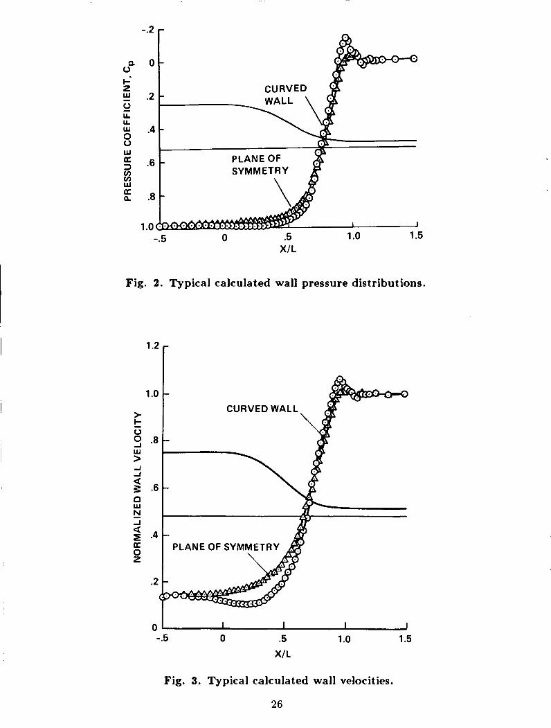
The calculated pressure distributions on the curved wall and centerline of a typical contraction are given in Fig. 2. On the whole, the pressure decreases through the strong favorable pressure gradient in the contraction, as would be expected. However, note the regions of adverse pressure gradient on the curved wall near the contraction inlet and outlet. These regions are more apparent in the wall velocity distributions shown in Fig. 3. rhe regions of adverse pressure gradient being indicated by a decrease in wall velocity.

3.2 Boundary Layer Codes

T h e surface velocities generated by VS.4ERO were used as input boundary conditions for tno different boundary layer codes - one using a simple integral method to solve the nio~tientum integral equation and the other employing a finite difference scheme to solve t h e boundary layer equations.

In all cases. it was assumed that the boundary layer originates from stagnation con- ditions at t h e start of the contraction. This is a new assumption and requires some justification. SOW in most small wind tunnels. the flow entering the contraction comes through a honeycomb and a series of screens (usually at least three). The effect of a screen on a turbulent boundary layer is to significantly reduce its thickness and turbulence stress levels and scales as shown by hlehta (1985). The results from that investigation showed t h a t a turbulent boundary layer a t moderate Reynolds riurnbers (Red - 1600) was effec- tively relaminarized immediately downstream of the screen. Note that the typical Red encountered in small. low-speed settling chambers is likely to be lower by at least a n order of magnitude. Furthermore, the fine scale, low-level turbulence generated in the screen wire wakes dissipates very rapidly (Mehta. 1985) and it is therefore not likely to trigger transition in the emerging boundary layer. However. it is still possible for the laminar boundary layer to undergo transition within the contraction, through either the effects of the Tal-lor-Gortler instabilities in the regions of concave curvature or a separation bub- ble. in which case transition would occur in the separated shear layer. In either case.

11

the strong favorable pressure gradient, encountered in contractions with reasonable area ratios (c - 6-10), would invariably relaminarize the boundary layer soon after. Therefore, the assumption of a laminar boundary layer originating from stagnation conditions at the contraction entrance and remaining laminar throughout was considered to be an adequate approximation for all cases.

The boundary layer was calculated along the centerline (in the spanwise reference) of the curved wall on the contraction. For the case of a mixing layer tunnel contraction, the boundary layer on the splitter plate was also calculated.

The VSAERO output was not entirely regular - glitches occured in the surface velocity output as a result of discontinuities across the panel boundaries. Although the irregularities were small. the effect of these glitches was magnified since both boundary layer codes used the velocity gradient as input. In an attempt to reduce these effects, the velocity gradient data were smoothed using an error detection routine. A typical example of the calculated velocity gradient and results of the smoothing procedure are shown in Fig. 4 . The routine compares each point with a cubic spline approximation based on the neighboring points, without including data from the point in question. Points which differ significantly from the cubic spline are moved toward the approximated line. The process is iterated until some defined smoothness is achieved.

The simpler boundary layer code (Thwaites method) consisted of an integral method to calculate the momentum thickness. The program itself is short and simple to use (see Cebeci and Bradshaw. 1977, p. After the momentum thickness is calculated the program uses semi-empirical relations for a laminar boundary layer in zero pressure gradient to evaluate the other boundary la!er parameters.

For comparison wi th the Thwaites' method, a relatively complex boundary layer code was also used. PDlIIXT acronym for Partial Differential Method Interactive - described in more detail by Alurphy and King (1982)i applies the generalized Galerkin method to a system of equations consisting of the momentum and continuity equations. Given the tran- sit ion location, PDM INT is capable of calculating both laminar and turbulent boundary layers. as well as separation bubbles. The code uses the Cebeci and Smith turbulence model w i t h o u t a correction for pressure gradient. Originally developed for transonic boundary layers. PDMINT turned out to be somewhat overly complex for the needs of the present study.

The momentum thickness and skin friction distributions calculated using both the boundary layer programs in a t ) pica1 " S U C C ~ S S ~ ~ ~ " contraction section are shown in Fig. 5 . Initially. the boundary layer grows rapidly in the inlet region where the effects of the first adverse pressure gradient are felt. This is soon overwhelmed by the effects of the strong favorable pressure gradient. resulting in a rapid reduction of the boundary layer thickness, before the effects due to the adverse gradient near the outlet take over. The skin friction coefficient remains well positive all through the contract ion. thus indicating that separation is not predicted for this particular design. The results from the two techniques are seen to compare favorably. especially for the region near t h e contraction outlet. The predictions given by the two computational methods agree to well within 10% in this region for both the plotted quantities. Since Thwaites' method is a lot simpler to obtain and use, almost all of the boundary layer calculations presented below were computed using this method. '4

114 for a source code listing).

12

negative, or very low value for the skin friction coefficient (5 0.0005) was taken to indicate boundary layer separation. An example of an unsuccessful design where the boundary layer separated near the inlet, is given in Fig. 6. Note that both boundary layer computations indicate that separation would occur in this particular design; the two computations also predict about the same streamwise location for the separation.

4. RESULTS AND DISCUSSION

4.1 Validation of Computational Scheme

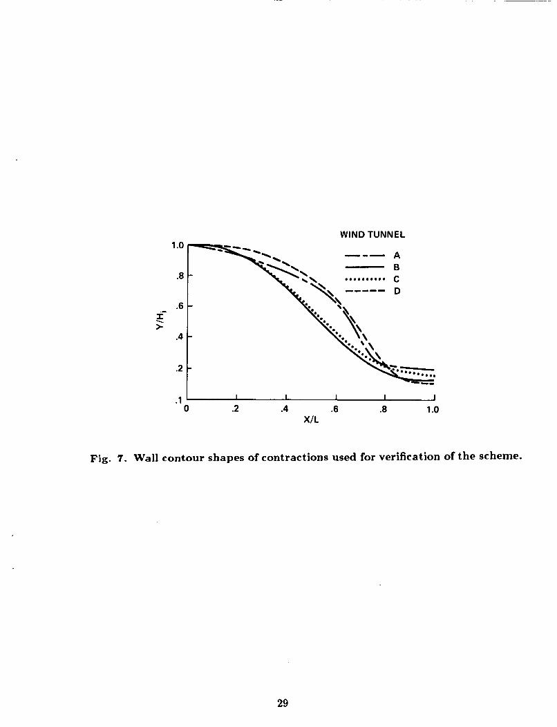
The combination of an inviscid panel code coupled with the boundary layer calcula- tions provides an estimate of the boundary layer quantities in the contraction section. In order to validate the proposed computational scheme, the boundary layer properties in four contractions installed on blower-driven (open-circuit) wind tunnels were calculated using this method. Details of the wind tunnel contraction sections are given in Table 1. The two wind tunnels with splitter plates in their contractions (A and B), were primar- ily designed for free-shear layer research. Wind tunnels A, B and C are located in the Fluid Mechanics Laboratory (FML) at NASA Ames Research Center and wind tunnel D is located in the Aeronautics Department at Imperial College. The act,ual wall shapes for the four contraction sections are plotted in a normalized form in Fig. i. Two of the wall shapes were based o n a 5th order polynomial while the other two were designed "by eye" using the guidelines described above in Section 3.

The computed wall pressure coefficients and calculated distributions of the boundary layer properties for all four contractions are given in Figs. 8-11. Boundary layer separation is not indicated for any of the contraction designs. The measured and calculated values of the boundary layer momentum thickness a t the exit of all four contractions are presented and compared in Table 2. The comparisons are made along the wind tunnel centerline at a shor t distance (typically less than 15 cm) downstream of the contraction esit. The values predicted by Thwaites' method for all four cases are within about lo'% of the measured values: t h e typical repeatibility for the measurements in wind tunnel B, for example, was about 1'7. The predicted values are generally lower than the measured ones because the 2-D boundary layer computation obviously cannot account for the weak secondary flow that develops along the contraction walls (Mokhtari and Bradshaw, 1983). This secondarj flow is a result of the lateral convergence of boundary layer fluid towards the local centerline forced by the converging sidewalls. This effect would therefore not occur in the boundary layer on the curved walls (in the streamwise sense) in a 2-D contraction where the sidewalls are straight. The effect of this secondary flow which is in the form of a pair of streamwise vortices with the "common flow" away from the wall is to thicken the boundary layer along the tunnel centerline (Mehta and Bradshaw, 1988). Note that the maximum difference between predictions and experiments occurs for wind tunnel A which also has the maximum three-dimensionality in the contraction geometry. I t is also worth noting that all the contractions discussed here have an aspect ratio of about five. I t is conceivable that for tunnels with smaller aspect ratios and longer lengths, the 2-

13

D boundary layer computations may not work as well since 3-D effects may then start to dominate. Comparisons for the other boundary layer quantities which are derived using empirical relations in Thwaites method are given in Table 3. On the whole, the agreement between the predicted and measured values is reasonable. It is worth noting that in Thwaites’ method, the momentum integral equation is reduced to a numerically integrable level (for e) by relating the momentum thickness to the shape factor and skin friction coefficient through quasi-similarity assumptions. The relationships are nonlinear and so the errors encountered in predicting the momentum thickness will typically tend to increase for the other quantities. On the whole, however, a reasonable quantitative description of the laminar boundary layer is predicted using this scheme. Fig. 12 shows the computed results for the 40:l contraction installed on the Smoke Tunnel which is also located in the FML a t NASA Ames. Since boundary layer separation is predicted at the inlet to this contraction, the computed data are not included in Tables 2 and 3. While we have not been able to establish clearly if separation does occur in this contraction, this result is perhaps not too surprising considering the relatively short length of this design (LIH, = .66) for the contraction ratio (c = 40).

4.2 Selection of Optimum Wall Shape

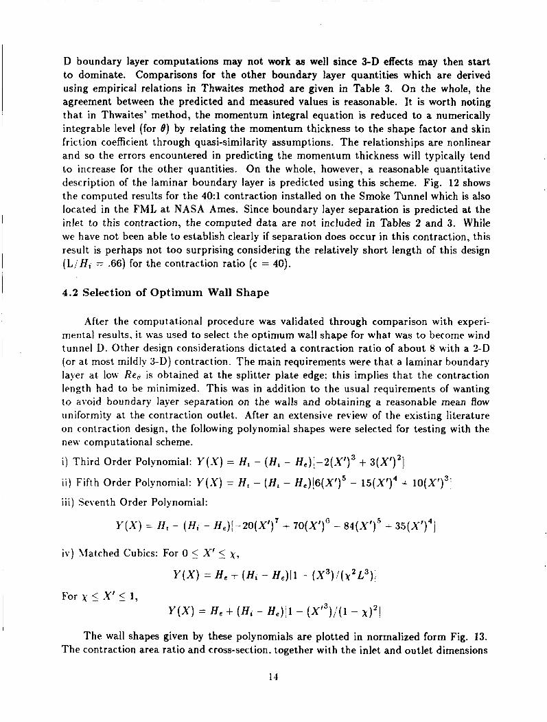
After the computational procedure was validated through comparison with experi- mental results, it was used to select the optimum wall shape for what was to become wind tunnel D. Other design considerat,ions dictated a contraction ratio of about 8 with a 2-D (or at most mildly 3-D) contraction. The main requirements were that a laminar boundary layer at low Re, is obtained at the splitter plate edge: this implies that the contraction length had to be minimized. This was in addition to the usual requirements of wanting to avoid boundary layer separation on the walls and obtaining a reasonable mean flow uniformity at the contraction outlet. After an extensive review of the existing literature on contraction design, the following polynomial shapes were selected for testing with the new computational scheme.

i ) Third Order Polynomial: Y ( X ) = H , - ( H , - Z I ~ ) ; - ~ ( X ’ ) ~ + 3(X’)’]

i i ) Fifth Order Polynomial: Y(.Y) = H , - ( H , - He)[6(X’)’ - 15(X’)4 + 10(X’)3]

i i i ) Seventh Order Polynomial:

Y ( X ) = H , - ( H , - H ~ ) ~ - ~ o ( x ‘ ) ’ + 70(X‘)(j - 8 q ~ ’ ) ~ 3 5 ( ~ ’ ) ~ j

The wall shapes given by these polynomials are plotted in normalized form Fig. 13. The contraction area ratio and cross-section. together with the inlet and outlet dimensions

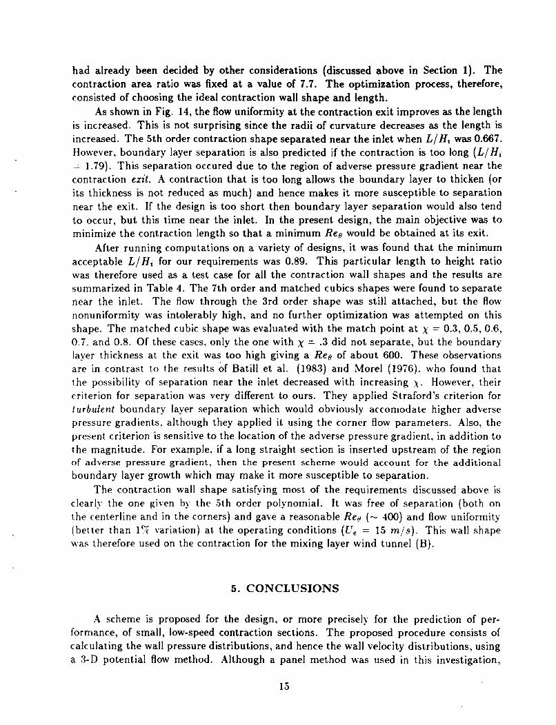
had already been decided by other considerations (discussed above in Section 1). The contraction area ratio was fixed at a value of 7.7. The optimization process, therefore, consisted of choosing the ideal contraction wall shape and length.

As shown in Fig. 14, the flow uniformity at the contraction exit improves as the length is increased. This is not surprising since the radii of curvature decreases as the length is increased. The 5th order contraction shape separated near the inlet when L / H , was 0.667. However, boundary layer separation is also predicted if the contraction is too long ( L / H , = 1.79). This separation occured due to the region of adverse pressure gradient near the contraction ezit. A contraction that is too long allows the boundary layer to thicken (or its thickness is not reduced as much) and hence makes it more susceptible to separation near the exit. If the design is too short then boundary layer separation would also tend to occur, but this time near the inlet. In the present design, the main objective was to minimize the contraction length so that a minimum Reo would be obtained at its exit.

After running computations on a variety of designs, it was found that the minimum acceptable L / H , for our requirements was 0.89. This particular length to height ratio was therefore used as a test case for all the contraction wall shapes and the results are summarized in Table 4. The 7th order and matched cubics shapes were found to separate near the inlet. The flow through the 3rd order shape was still attached, but the flow nonuniformity was intolerably high, and no further optimization was attempted on this shape. The matched cubic shape was evaluated with the match point a t x = 0.3, 0.5, 0.6, 0.7, and 0.8. Of these cases, only the one with x = .3 did not separate, but the boundary layer thickness at the exit was too high giving a Reo of about 600. These observations are in contrast to the results of Batill et al. (1983) and Morel (1976), who found that t h e possibility of separation near the inlet decreased with increasing x. However, their criterion for separation was very different to ours. They applied Straford’s criterion for t u r b u l e n t boundary layer separation which would obviously accomodate higher adverse pressure gradients. although they applied it using the corner flow parameters. Also, the present criterion is sensitive to the location of the adverse pressure gradient, in addition to the magnitude. For example. if a long straight section is inserted upstream of the region of adverse pressure gradient, then t h e present scheme would account for the additional boundary layer growth which may make it more s~scept~ible to separation.

The contraction wall shape satisfying most of the requirements discussed above is clear]\- t h e one given bx the 5th order polynomial. I t was free of separation (both on the centerline and in the corners) and gave a reasonable Red ( - 400) and flow uniformity (better t h a n l? variation) at the operating conditions (Cr, = 15 rn / s ) . This wall shape was therefore used on the contraction for the mixing layer wind tunnel (B).

5. CONCLUSIONS

A scheme is proposed for the design, or more precisely for the prediction of per- formance, of small, low-speed contraction sections. The proposed procedure consists of calculating the wall pressure distributions, and hence the wall velocity distributions, using a 3-D potential flow method. Although a panel method was used in this investigation,

in principle any potential flow solver should be acceptable. Once the wall pressures and velocities have been obtained, the boundary layer behavior can be adequately calculated rather than relying on some separation criteria based on the pressure coefficients, as has been the normal practice in the past. For the family of contractions discussed in this note, the assumption of a laminar boundary layer originating at the contraction entrance and remaining laminar in passage through it seems justified. The measured boundary layer momentum thicknesses a t the exit of four existing contractions, two of which were 3-D, were found to lie within 10% of the predicted values, with the predicted values generally lower. Although more sophisticated boundary layer codes could be used, the present re- sults indicate that the relatively simple Thwaites integral method is probably adequate for most purposes. If the prediction accuracy of within 10% on 8 is acceptable, then the present results also suggest that an iterative process for the wall pressure computations, accounting for the boundary layer displacement thickness, is not necessary. From the con- traction designs investigated, the wall shape based on a 5th order polynomial was found to perform optimally in terms of avoiding separation and giving minimum Re@ and flow nonuniformity.

Until further data are obtained, all these conclusions should be confined to small (test section area 5 0.5 m 2 ) , low-speed ( V , 5 4 0 m / s ) contractions with area ratios of around eight, exit aspect ratios of about five and length to inlet height ratios of about one.

ACKNOWLEDGEMENTS

We are grateful to Lawrence Olson for making arrangements which allowed us to use the \'S.\ERO computer program and to Dale Ashby for the considerable help in running it. \ l e would also like to thank John Murphy for giving us access to the PDMINT boundary layer code and the help and advice in using it. We are indebted to thank Russell Westphal and David Wood for providing the boundary layer data for two of the wind tunnels. This work was supported by the Fluid Dynamics Research Branch. N.4SA Ames Research Center under grant NCC-2-294.

REFERENCES

Rarger. R.L. and Bowen, J.T., "-4 Generalized Theory for the Design of Contraction Cones and Other Low-Speed Ducts," NASA TN D-6962, hovember 1973.

Batchelor, G. K., "The Theory of Homogeneous Turbulence,'' Cambridge University Press? 1953, pp 68-75.

Batill, S. M., Caylor, M.J. and Hoffman, J.J., "An Experimental and Analytic Study of the Flow in Subsonic Wind Tunnel Inlets,* Air Force Wright Aeronautical Laboratories TR-83-3109, October 1983.

16

Batill, S. M. and Hoffman, J.J., "Aerodynamic Design of Three-dimensional Subsonic Wind Tunnel Inlets," A I A A J., Vol. 24, No. 2, February 1986, pp. 268-269.

Bloomer, N.T., "Notes on the Mathematical Design of Nozzles and Wind Tunnel Contrac- tions,? Aeronaut. Q., Vol. 8, 1957, pp. 274290.

Borger, G.G., "The Optimization of Wind Tunnel Contractions for the Subsonic Range," NASA TT F-16899, March 1976.

Bossel, H.H., "Computation of Axisymmetric Contractions," A I A A J., Vol. 7, No. 10, 1969, pp 2017-2020.

Bradshaw, P. and Pankhurst, R.C., "The Design of Low-Speed Wind Tunnels," Prog. Aerospace Sei., Vol. 5 , 1964, p. 1.

Bradshaw, P., "Experimental Fluid Dynamics," Pergamon Press, Oxford, 1970.

Bradshaw, P. "Effects of Streamline Curvature on Turbulent Flow," AGARDograph 169, 1973.

Bradshaw, P., "Two more Wind Tunnels Driven by Aerofoil-Type Centrifugal Blowers," Imperial College Aero. Report 72-10, 1972.

Cebeci. T. and Bradshaw, P., "Momentum Transfer in Boundary Layers," Hemisphere Publishing Co.. 1977.

Cheers. F.. "Notes on Wind-tunnel Contractions," Aeronautical Research Council Reports and ylemorandum No. 2137, March 1945.

Chmielewski, G .E., "Boundary-Layer Considerations in the Design of Aerodynamic Con- tractions:" J. .4ircraft. Vol. 11. No. 8, 1974, pp. 435-438.

Cohen. M. J. and Ritchie. S. J . B., "Low-speed Three-dimensional Contract,ion Design.? J. Roy. Aeronaut. SOC., No. 66, 1962, p. 231.

Downie. J.H.. Jordinson. R. and Barnes, F.H., "On the Design of Three-Dimensional Wind Tunnel Contractions." Aeronaut. J., i.01. 88, 1984. pp. 287-295.

Gay, B.. Spettel. F., Jeandel, D. and Mathieu, J., "On the Design of the Contraction Section for a Wind Tunnel," ASME J. Applied Mech., Series E. Vol. 40. So. 1 , 1973. pp. 309- 3 1 0.

Gibbings. J . C. and Dixon, J. R., "Two-dimensional Contracting Duct Flow," Q. J. Meeh. . 4 p p / . .\daih.. Voi. 10, Part 1, February 1957, pp 24-41.

Gibbings. J. C., "Flow in Contracting Ducts," AZAA J., Vol. 2, No. 1 , January 1964, pp. 191- 192.

Gibbings. J . C., "The Choice of a Hodograph Boundary for Contracting Ducts: J. Roy. Aeronaut. SOC., Vol. 68, No. 6, June 1964, pp. 420-432.

17

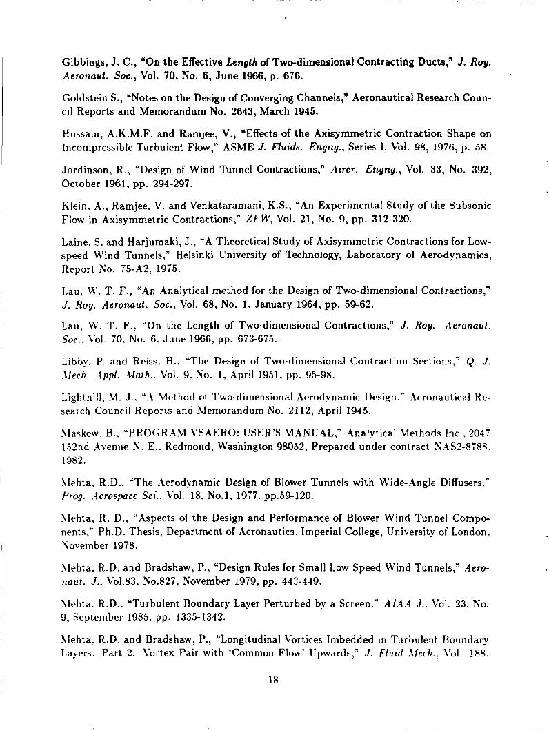
Gibbings, J. C., “On the Effective Length of Twedimensional Contracting Ducts,” J. Roy. Aeronaut. SOC., Vol. 70, No. 6, June 1966, p. 676.

Goldstein S., “Notes on the Design of Converging Channels,” Aeronautical Research Coun- cil Reports and Memorandum No. 2643, March 1945.

Hussain, A.K.M.F. and Ramjee, V., “Effects of the Axisymmetric Contraction Shape on Incompressible Turbulent Flow,” ASME J . Fluids. Engng., Series I, Vol. 98, 1976, p. 58.

, Jordinson, R., “Design of Wind Tunnel Contractions,” Airct. Engng., Vol. 33, No. 392, October 1961, pp. 294-297.

Klein, A., Ramjee, V. and Venkataramani, K.S., “An Experimental Study of the Subsonic Flow in Axisymmetric Contractions,” Z F W , Vol. 21, No. 9, pp. 312-320.

Laine, S. and Harjumaki, J., “A Theoretical Study of Axisymmetric Contractions for Low- speed Wind Tunnels,” Helsinki University of Technology, Laboratory of Aerodynamics, Report Yo. 75-A2. 1975.

Lau. M’. T. F., “An Analytical method for the Design of Two-dimensional Contractions,” J . Roy. Aeronaut. Soe., Vol. 68, No. 1, January 1964, pp. 59-62.

Lau, W. T. F., “On the Length of Two-dimensional Contractions,” J . Roy. Aeronaut. Soc.. Vol. 70, No. 6. June 1966, pp. 673-675.

Libby. P. and Reiss. H., “The ‘Design of Two-dimensional Contraction Sections,” Q. J. -1fec.h. -4pp l . . tfath.. Vol. 9, Yo. 1, April 1951, pp. 95-98.

, Lighthill. M. J.. ‘‘.4 Method of Two-dimensional Aerodynamic Design.” -4eronautical Re- search Council Reports and Memorandum Eo. 2112, April 1945.

I llaskew. B., “PROGRAM VSAERO: USER’S MANUAL,” Analytical Methods Inc.. 2047 152nd Avenue N. E.. Redmond, Washington 98052, Prepared under contract NAS2-8788. 1982.

I lfehta. R.D.. ”The -4erodynamic Design of Blower Tunnels with Wide-Angle Diffusers.” Prog. .-terospce Sci., Vol. 18, No.1, 1977. pp.59-120.

l lehta, R. D., “Aspects of the Design and Performance of Blower Wind Tunnel Compo- nents,” Ph.D. Thesis, Department of Aeronautics. Imperial College, University of London.

I Sovember 1978.

llehta. R.D. and Bradshaw, P., “Design Rules for Small Low Speed Wind Tunnels,? Aero- J.. Vo1.83. 30.827. November 1979, pp. 443-119.

llehta. R.D.. “Turbulent Boundary Layer Perturbed by a Screen.’ AIAA J., Vol. 23, So. 9, September 1985, pp. 1335-1342.

I Ilehta, R.D. and Bradshaw, P., “Longitudinal Vortices Imbedded in Turbulent Boundary Layers. Part 2. Vortex Pair with ‘Common Flow’ Upwards,” J. Fluid ‘2lech.. 1’01. 188.

I 18

Mills, R. D., "Some Finite Two-cimensional Contractions," Aeronaut. Q., Vol. 19, Febru- ary 1968, pp. 91-104.

Mikhail, N. and Rainbird, W. J., "Optimum Design of Wind Tunnel Contractions,n AIAA Paper 78-819, 1978.

Mikhail, M.N., "Optimum Design of Wind Tunnel Contractions," AIAA J., Vol. 17, No. 5, 1979, pp. 471-477.

Mokhtari, S. and Bradshaw, P., "Longitudinal Vortices in Wind Tunnel Wall Boundary Layers," Aeronaut. J., Vo1.87, 1983, pp. 233-236.

Morel, T., "Comprehensive Design of Axisymmetric Wind Tunnel Contractions," ASME J. Fluids Engng., June 1975, pp. 225-233.

Morel, T., "Design of Two-dimensional Wind Tunnel Contractions," ASME Paper No. 76-WA/FE-4, December 1976, pp. 1-7.

Murphy, J. D. and King, L. S., "Airfoil Flow-field Calculations with Coupled Boundary- layer Potential Codes," Proceedings 2nd Conference on Numerical and Physical Aspects of Aerodynamic Flows, California State University, Long Beach, California, 1982.

Ross, J . C., Olson, L.E., hleyn. L.A. and Van Aken, J.M., "A New Design Concept for Indraft Wind-Tunnel lnlet<s with Application to the National Full-Scale -4erodynamics Complex." AI.4.A Paper 86-0043, January 1986.

Smith. -4. 31. 0. and Pierce. J., "Exact Solution of the Neumann Problem. Calculation of Non-circulatory Plane and .Axially Symmetric Flows About or Within Arbitrary Bound- aries," Douglas Aircraft Inc. Report ES 26988, 1959.

Smith. R. and Wang, C., Tontracting Cones Giving Uniform Throat Speeds." J. rleronaut. Sci . . Vol. 11, Yo. 4, October 1941, pp. 356360.

Stratford, B.S.. "The Prediction of Separation of the Turbulent Boundary Layer." J. Flutd .\lech.. 1-01. 5, 1959. pp. 1-16.

Swam}. Y. S. N.. "On the Design of a Two-dimensional Contracting Channel," J. '4erospace Sct . . Vole 28, No. 6, June 1961. pp. 500-501.

Swam}. Y. S. 3.. "A Note on the Design of a Two-diniensional Contracting Channel." J. .-Ierospaee Sci., Vol. 29, No. 3. February 1962, p. 246.

Szczeniowski, B., "Contraction Cone for a Wind Tunnel," J. .4eronaut. Sci. Vol 10, So. 8. October 1943, p. 311.

Szczeniowski. B., "Further Note on the Design of Two-dimensional Contracting Channels," AI.4.4 J. C'ol. 1, No. 4, April 1963, p. 977.

Thwaites. B.. "On the Design of Contractions for Wind Tunnels." Aeronautical Research

19

Council Reports and Memorandum No. 2278, 1946.

Tsien, H., “On the Design of the Contraction Cone for a Wind Tunnel,” J. Aeronaut. Sci. Vol. 10, No. 2, February 1943, pp. 68-70.

Tulapurkara, E.G., “Studies on Thwaites’ Method for Wind Tunnel Contraction,” Aero- naut. J., Vol. 84, 1980, pp. 167-169.

I Tulapurkara, E.G. and Bhalla, V.V.K., “Experimental Investigation of Morel’s Method for Wind Tunnel Contractions,” J. Ffuids Engng., Vol. 110, 1988, pp. 45-47.

Watmuff, J. H., “Wind Tunnel Contraction Design,” Proceedings 9th Australasian Fluid Mechanics Conference, Auckland, New Zealand, December 1986.

Whitehead, L. G., Wu, L. Y. and Waters, M. H. L., “Contracting Ducts of Finite Length,” Aeronaut. Q., Vol. 2, 1951, p. 254.

Wood, D.H., “A Reattaching, Turbulent, Thin Shear Layer,” Ph.D. Thesis, Department of Aeronautics, Imperial College, London University, January 1980.

W700d, D.H. and Westphal, R.V., “Potential Flow Fluctuations Above a Turbulent Bound- ary Layer,” NASA-TM 100036, November, 1987.

I

20

> z z

d Y In

9 m 9

d cn z 0 cn z a n 5 0 0 a 0 n IL

w cn 3 cn z 0 F 0 a a I- z 0 0 s Y zi n I- w

O a O &OCi a

N a N 2 2

m k h

0

21

ae F I

z 9 0

m a N o 0 * ( v 9 9

F C 3 oo

0 0

s : * 9 9

0 0

m o o G S 9 9 0 0

( D N d m 0 0 9 9

m (v i

A - - A P P n e

e o

a m n 0

22

d P O N r 00

0 0 9 9

(00 m a c o b 0 0 0 0 0 0

( V r ab, N O 00

00 9 9

O b m m 0 0

0 0

r r

9 9 0 0

iP K

N m b m m m m o $ 8

moo

r N

N m N N L n c q

moo

N N mcq I

0 0 0 QON m m 0 0

* Lo

0 0

m a m m 22 m W J

I-

m a W I) J

> W I-

a n

o n

n

n

3

> P W U 3 v)

W

I t

W K

II

.. w J a

a E

E

n E \ Z n E n E n

m m N

J

a m 0 n I-

23

TABLE 4

COMPARISON OF WALL SHAPE PERFORMANCE

SEPARATION PREDICTED

I EXIT PLANE Reo AT UNIFORMITY

CONTRACTJON EXIT (STANDARD DEVIATION)

CONTRACTION WALL SHAPE

NO POLYNOMIAL 1 3RD0RDER 359 0.0102

5TH ORDER POLYNOMIAL

NO

YES

YES

7TH ORDER POLYNOMIAL

428 0.0040

478 0.0024

484 0.0024 SYMMETRIC MATCHED CUBICS

CONTRACTION RATIO = 7.7, LENGTH TO HEIGHT RATIO = 0.89, FREE-STREAM VELOCITY = 15 m/sec

24

u a x .I

*

E

a ." A

25

-.2

a 0 0

2

0

w .4

I--

2 .2 - LL LL

8

3

W a 3

W

.8

1 .o -.5 0 .5 1 .o 1.5

X/L

Fig. 2. Typical calculated wall pressure distributions.

I I 1 I -.5 0 .5 1 .o 1.5

XIL

Fig. 3. Typical calculated wall velocities.

26

a 1.5

3 '0

P

\

I-

W 1.0 -

0 a a (3 .5

9 -.5

RAW DATA ---

1 I I I 1 1 0 .4 .8 1.2 1.6 2.0

NORMALIZED DISTANCE ALONG WALL, S/L

Fig. 4. Example of smoothing used on velocity gradient data.

27

c I z .010 - X THWAITES PDMINT E ". .008

z a n a .oo6 0' K

> .004

4 g .002 a n 3 0 z

-.25 0 .25 .50 .75 1.0 1.25 1.50

X/L

Fig. 5. Calculation of boundary layer development through a contrac

7 .015 0

X r

Y

E ". .010

0 z a 0' .005 K w > -I

Q

a > 0 a a 0 z 3

-.005

THWAITES PDMINT

0 .4 .a 1.2 1.6 X I L

,tion.

Fig. 6. Boundary layer calculation indicating separation.

28

1 .o

.8

.6 .- I > \

.4

.2

WIND TUNNEL

--- A

- .......... c

-

-

-

. I -

0 .2 .4 .6 .8 1 .o X/L

Fig. 7 . Wall contour shapes of contractions used for verification of the scheme.

29

0

.2

cp .4

.6

.8

1 .o

.012

.010

.008

5 .006

2 .004

.002

F

b X - m n a z

-.5 0 .5 1 .o 1.5 X/L

-

-

-

-

-

-

THWAITES METHOD oe 0 Cf

0 ' k I I I 1

0 .4 .8 1.2 .16 XJL

Fig. 8. Wall pressure distributions and boundary layer calculations for the contraction on wind tunnel A.

30

.010

.008 F I

2 x .006 - E V

-.5 0 .5 1 .o 1.5 X I L

THWAITES METHOD 0 8 0 Cf

a- n .004 z a 6- .002

0 Y .

0 .4 .8 1.2 1.6 X/L

Fig. 9. Wall pressure distributions and boundary layer calculations for the contraction on wind tunnel B.

31

-.2

0

.2

cp .4

.6

.8

7.0'

m

PLANE OF

-.5 0 .5 1 .o 1.5 X/L

THWAITES METHOD .010 r - .008 r

b r

5 .006 E 0

0

0 8

0 Cf

0 .4 .8 1.2 1.6 X/L

Fig. 10. Wall pressure distributions and boundary layer calculations for the contraction on wind tunnel C.

32

-.2

0

.2

cp .4

.6

.8

1.0 -.5 0 .5 1 .o 1.5

X/L

.014

g.2 .012

.006 a

.004

.002

0

r THWAITES METHOD oe

0 .4 .8 1.2 1.6 X/L

Fig. 11. Wall pressure distributions and boundary layer calculations for the contraction on wind tunnel D.

33

-.2

0

.2

cp .4

.6

.8

1 .O' - 0 .5 1 .o 1.5 XI L

.06 A

F I

v- 0

THWAITES METHOD ne 0 Cf

-.02 I I I 1 I 1 0 .4 .8 1.2 1.6

X I L

Fig. 12. Wall pressure distributions and boundary layer calculations for the contraction on the Smoke Tunnel.

34

WALL CONTOUR SHAPE --- 3RD ORDER POLYNOMIAL . . . . . . . 5TH ORDER POLYNOMIAL

--- 7TH ORDER POLYNOMIAL 1 .oo

.75

.25

L I 1 I 1 I -1 0 .25 .50 .75 1 .oo

X/L

Fig. 13. Wall contour shapes of contractions tested.

35

1.6

s 1.2 -

0 0 J W > W z J K W

- I- .8 5 0 I 0 K

z 0 I-

>

L

- 5 .4 W n

0 .6

0 ATTACHED

0 SEPARATED BOUNDARY LAYER

BOUNDARY LAYER

1 .o 1.4 L/H i

1.8

Fig. 14. Effect of contraction length on flow uniformity.

36

1. Report No.

N A S A C R 177488

James H. B e l l R a b i n d r a D. Mehta

2. Government Accession No. 3. Recipient's Catalog No.

10. Work Unit No.

4. Title and Subtitle

C o n t r a c t i o n D e s i g n f o r S m a l l Low-Speed Wind T u n n e l s

7. Author(s1

5. Report Date

A t 1 9 8 8 6. Performwrganization Code

8. Performing Organization Report No.

N a t i o n a l A e r o n a u t i c s a n d S p a c e A d m i n i s t r a t i o W a s h i n g t o n , D.C. 20546

9. Performing Organization Name and Address

S t a n f o r d U n i v e r s i t y S t a n f o r d , C A 94305

12. Sponsoring Agency Name and Address

I

15. Supplementary Notes

- - 11. Contract or Grant No.

- - 13. Type of Report and Period Covered

P o i n t o f C o n t a c t : L. S. K i n g , M.S. 260-1, Moffe t t F i e l d , C A 94035 (415)694-6116 o r FTS 464-6116

16.Abstract An i t e r a t i v e d e s i g n p r o c e d u r e h a s b e e n d e v e l o p e d f o r t w o - o r t h r e e - d i m e n s i o n a l c o n t r a c t i o n s i n s t a l l e d o n s m a l l , l o w - s p e e d w i n d t u n n e l s . T h e p r o c e d u r e c o n s i s t s o f f i r s t c o m p u t i n g t h e p o t e n t i a l f l o w f i e l d a n d h e n c e t h e p r e s s u r e d i s t r i b u t i o n s a l o n g t h e w a l l s o f a c o n t r a c t i o n o f g i v e n s i z e a n d s h a p e u s i n g a t h r e e - d i m e n s i o n a l n u m e r i c a l p a n e l me thod . T h e p r e s s u r e o r v e l o c i t y d i s t r i b u t i o n s a r e t h e n f e d i n t o t w o - d i m e n s i o n a l b o u n d a r y l a y e r c o d e s t o p r e d i c t t h e b e h a v i o r o f t h e b o u n d a r y l a y e r s a l o n g t h e wal ls . F o r s m a l l , l o w - s p e e d c o n t r a c t i o n s i t is s h o w n t h a t t h e a s s u m p t i o n o f a l a m i n a r b o u n d a r y l a y e r o r i g i n a t i n g from s t a g n a t i o n c o n d i t i o n s a t t h e c o n t r a c t i o n e n t r y a n d r e m a i n i n g l a m i n a r t h r o u g h o u t p a s s a g e t h r o u g h t h e " s u c c e s s f u l " d e s i g n s I s j u s t i f i e d . T h i s h y p o t h e s i s was c o n f i r m e d by c o m p a r i n g t h e p r e d i c t e d b o u n d a r y l a y e r d a t a a t t h e c o n t r a c t i o n e x i t w i t h m e a s u r e d d a t a i n e x i s t i n g w i n d t u n n e l s . The m e a s u r e d b o u n d a r y l a y e r momentum t h i c k n e s s e s a t t h e e x i t of f o u r e x i s t i n g c o n t r a c t i o n s , two o f w h i c h were 3-0, were f o u n d t o l i e w i t h i n 10% o f t h e p r e d i c t e d v a l u e s , w i t h t h e p r e d i c t e d v a l u e s g e n e r a l l y lower.

9. Security Classif. (of this report)

'7. Key Words (Suggested by AuthorM)

20. Security Classif. (of t

37 U n c l a s s i f i e d U n c l a s s i f i e d

18. Distribution Statement

A02

Un 1 i m i t e d STAR C a t e g o r y 34

s page) I 21. No. of pages 1 22. Price