Beliefs and Voting Decisions: A Test of the Pivotal Voter Model

Beliefs and Voting Decisions: A Testof the Pivotal Voter Model

John Duffy George Mason UniversityMargit Tavits Washington University in St. Louis

We report results from a laboratory experiment testing the basic hypothesis embedded in various rational voter models thatthere is a direct correlation between the strength of an individual’s belief that his or her vote will be pivotal and the likelihoodthat individual incurs the cost to vote. This belief is typically unobservable. In one of our experimental treatments we elicitthese subjective beliefs using a proper scoring rule that induces truthful revelation of beliefs. This allows us to directly test thepivotal voter model. We find that a higher subjective probability of being pivotal increases the likelihood that an individualvotes, but the probability thresholds used by subjects are not as crisp as the theory would predict. There is some evidence thatindividuals learn over time to adjust their beliefs to be more consistent with the historical frequency of pivotality. However,many subjects keep substantially overestimating their probability of being pivotal.

Why do people vote? While many theories havebeen offered (for a survey see Dhillon and Per-alta 2002), the simplest and most widely used

framework is the pivotal voter model (Ledyard 1984; Pal-frey and Rosenthal 1983, 1985; see also Downs 1957; Tul-lock 1967). This model asserts that voters have only instru-mental concerns—their motivation is to affect the out-come of the election as opposed to noninstrumental mo-tivations, such as warm-glow altruism—and that in mak-ing the decision to vote they are rational, self-interestedexpected payoff maximizers. In particular, people vote ifthe expected benefit of voting is greater than the cost.

This model has widespread appeal but it is simulta-neously the most extensively debated theory in politicalscience (Green and Shapiro 1994, 47–48). The problem isstraightforward: the expected benefit calculation involvesthe voter’s probability that he or she will be pivotal to theelection outcome. As in large electorates, where this prob-ability is very small, rational citizens should not vote. This,however, contradicts the evidence. It is this paradox thatfeeds the rational choice controversy (Friedman 1995).Indeed, the apparent anomaly has led to the search for an

John Duffy is professor of economics, George Mason University, 4400 University Drive, MSN 3G4, Fairfax, VA 22030 ([email protected]).Margit Tavits is professor of political science, Washington University in St. Louis, Campus Box 1063, One Brookings Drive, St. Louis, MO63130 ([email protected]).

We thank Scott Kinross and Jonathan Lafky for expert research assistance. We have benefited from the helpful comments of James Adams,Taavi Annus, Marco Battaglini, Mark Andreas Kayser, Michael McClurg, Jack Ochs, and Jonathan Williamson and audiences at the 2006annual meetings of the Midwest Political Science Association and the American Political Science Association, and the 2007 annual meetingof the American Economic Association.

extra term—the “D-term” or “a sense of civic duty”—tomake voting rational (Riker and Ordeshook 1968). How-ever, this explanation remains theoretically unrewarding(Bendor, Diermeier, and Ting 2003).

Given this central controversy in the discipline, it iscurious that empirical studies examining the assumptionsand predictions of the pivotal voter model are scarce andindirect. Field data can usually provide only weak tests ofthe model as they pose challenge to measurement and pro-vide little control over extraneous factors (see Levine andPalfrey 2007). Among the difficulties are the unobserv-ability of voters’ costs of voting, benefits from an electionvictory, and their beliefs as to whether they will be pivotalto the election outcome—all of which play a critical rolein the theory (Green and Shapiro 1994, 47–71).

Undoubtedly, the greatest controversy surrounds themeasurement and relevance of the probability of any voterbeing pivotal—the trademark of the rational choice the-ory of turnout (Aldrich 1993; Foster 1984; Green andShapiro 1994, 47–71). Various proxies have been usedto measure pivotality, such as the expected or perceivedcloseness of the election (Blais and Young 1999; Blais,

American Journal of Political Science, Vol. 52, No. 3, July 2008, Pp. 603–618

C©2008, Midwest Political Science Association ISSN 0092-5853

603

604 JOHN DUFFY AND MARGIT TAVITS

Young, and Lapp 2000; Ferejohn and Fiorina 1975; Foster1984; see also Matsusaka and Palda 1993 for a review) andthe size of the electorate (Hansen, Palfrey, and Rosenthal1987; see also Bendor, Diermeier, and Ting 2003, 274–75). However, these proxies have been criticized as beinga “far cry” from the actual concept of pivotality (Aldrich1993, 259; Cyr 1975, 25; Green and Shapiro 1994, 54–55; Shachar and Nalebuff 1999). Survey measures, suchas whether the respondent has thought of the possibilitythat his or her vote might decide the election, or whetherthe respondent thinks the probability of such an eventis higher than “absolute zero” or “almost zero” (Blais,Young, and Lapp 2000), or replacing decisiveness by po-litical efficacy (Clarke et al. 2004) provide interesting in-sights into turnout decisions, but remain imprecise formeasuring pivotality. Thus, the tests based on these prox-ies cannot be considered as tests of the pivotal voter model(Merlo 2006).1

An alternative to working with field data is to con-duct laboratory experiments that enable one to controlboth the cost of voting and the payoff to the party thatwins. Using neutral language and anonymous interactionexperiments can minimize other factors that might affectvoting decisions, such as the fulfillment of “civic duty”or the avoidance of peer sanctions for nonparticipation.Several prior experimental studies have tested various as-pects of the pivotal voter model, including the implica-tions of different voting rules (plurality vs. proportional)(Schram and Sonnemans 1996a), communication, groupidentity, and individual characteristics such as the stu-dent’s university major (Schram and Sonnemans 1996b),various comparative static predictions including the ef-fects of variations in electorate sizes (Großer, Kugler, andSchram 2005; Levine and Palfrey 2007), exogenously vary-ing the pivot probabilities by designating active individu-als whose vote determines the outcome (Feddersen, Gail-mard, and Sandroni 2007), and asymmetric information(Battaglini, Morton, and Palfrey 2005). However, none ofthese prior studies has examined subjects’ beliefs aboutbeing pivotal and assessed the extent to which subjects(1) form correct beliefs and (2) appropriately conditiontheir behavior on those beliefs—questions that lie at theheart of the pivotal voter model.

In this article, we present results from a series of labo-ratory experiments. We adopt the neutral language partic-ipation game design (Großer and Schram 2006; Schram

1Coate, Conlin, and Moro (2004) test the pivotal voter model bylooking at turnout in local Texas elections and considering closenessas a measure of pivotality. However, as above, this does not providea direct test of the model. See also Battaglini, Morton, and Palfrey(2005, 21) on how such tests are not nuanced enough as tests of thepivotal voter model.

and Sonnemans 1996a, 1996b)2 and add to it a belief elic-itation stage that precedes the voting stage. In the beliefelicitation stage, we ask subjects to state a subjective prob-ability as to whether their own decision to vote or not willbe decisive for the election outcome. We incentivize truth-ful revelation of individual beliefs using a proper scoringrule, and subject earnings are determined in small part bythe ex post accordance of their beliefs with election out-comes.3 In addition, we are able to study whether subjectslearn over time to form correct beliefs with regard to theirpivotality in the finitely repeated election game. In sum,our study provides the first direct test of the pivotal votermodel.

We find that average participation rates are consistentwith the theoretical prediction, suggesting that the modelworks well on an aggregate level. However, our main in-terest is on the individual level. Here we provide evidencethat subjects are more likely to vote the higher their subjec-tive beliefs of being pivotal—as prescribed by the pivotalvoter model. The predicted probability of participating ismore then twice as high for those who are certain of be-ing pivotal than for those who believe that their chance ofbeing pivotal is zero. On the other hand, we find that sub-jects consistently overestimated the probability that theirdecision to vote or abstain would be pivotal, though thisdifference declined somewhat with experience. Further-more, the fit between their beliefs about decisiveness andturnout was considerably worse than the theory predicted:many subjects whose perceived pivotality probability washigher than the cost of voting did not vote while manyof those who stated a probability considerably lower thanthe cost of voting still decided to participate.4 Overall,thus, the evidence with regard to the pivotal voter modelis mixed. Yet, the study should not be interpreted as anattempt to “prove” or “disprove” the pivotal voter modelor the rational choice theory in general. Rather, the pur-pose has been to uncover those aspects of the theory thatare useful for understanding turnout decisions.

2See Palfrey and Rosenthal (1983) and Schram and Sonnemans(1996a) for a justification why turnout decision can be representedas a participation game.

3Several other experimental studies have sought to elicit subjects’subjective beliefs in environments other than the voting game thatwe examine (Costa-Gomes and Weizsacker 2005; Croson 2000;McKelvey and Page 1990; Nyarko and Schotter 2002; Offerman,Sonnemans, and Schram 1996; Rutstrom and Wilcox 2004). Theevidence from these studies regarding the impact of belief elicitationprocedures on subject behavior is mixed. For this reason, we reportdata from our own control treatment without belief elicitation forthe purposes of comparison.

4As detailed below, we normalized the benefits from one’s preferredcandidate winning to one and set the cost of voting to 0.18.

BELIEFS AND VOTING DECISIONS 605

Our findings are for small groups of 20 subjects. Anobvious issue is whether our experimental findings “scaleup” to larger electorate sizes, where the probability of be-ing pivotal is likely to be closer to zero. We see no reasonwhy our findings should not scale up, but acknowledgethat this claim is difficult to test.5 Conducting controlledlaboratory experiments with much larger populations isnot presently feasible; Internet experiments do not pro-vide the same level of control, as one cannot rule outcommunication or collusion among subjects, and surveyevidence is not directly comparable to laboratory findings.

On the other hand, the laboratory provides the piv-otal voter theory with an idealized test environment—onewhere factors other than pivotality (such as civic duty orthe sanction of others) have been carefully removed, andwhere subjects are given much more experience and infor-mation concerning election outcomes and pivotality thanthey might ordinarily encounter as voters in real elections.If the theory does not predict well in this idealized envi-ronment (with admittedly few participants), we mightexpect it to perform rather poorly in the less-controlledworld of real elections with large numbers of participants.

Pivotal Voter Model

We consider the complete information participation gameapproach to modeling voting pursued by Palfrey andRosenthal (1983). Specifically, there are two teams of play-ers of size M and N , and all team members have a choicebetween two actions, vote (participation) or do not vote(abstention/nonparticipation). The cost of voting c ∈ (0,1) is assumed to be the same for all agents; abstention iscostless. Each member of the winning team receives a pay-off benefit B > 0, while each member of the losing teamearns a payoff of zero. The utility function is assumed tobe linear, as is standard in the literature. Specifically, let-ting p denote the probability of casting a pivotal vote, thenet return to voting, R = pB − c . Note that we abstractaway from any fixed benefits to voting, such as the utilityone gets from a “civic duty” to vote or from the avoid-ance of sanctions from not voting; our neutral languageexperimental design makes such concerns unimportant.Normalizing B = 1, it follows that players will rationallychoose to vote whenever p > c , and will rationally chooseto abstain if p < c .

5As Borgers (2004, 57) observes, “This paradox [of voting] suggeststhat a conventional game-theoretic analysis of costly voting is out ofplace if large electorates are considered. By contrast, for small elec-torates there seems to be no reason why observed voting behaviorshould not be rational.”

The rule used to determine the outcome of voting issimple plurality. As for ties, we flipped a coin in advanceof each election to determine which team would win inthe event of a tie; the pre-announcement of the winnerin the event of a tie aids in assessments of pivotality (asdescribed later). Given the pre-announcement of the tie-breaking rule, the setting corresponds to the “status quo”rule where there is a default winner in the event of a tie.

For our setting with M = N > 0 and the status quorule, it follows from Palfrey and Rosenthal (1983) thatthere are no pure strategy equilibria. There may existquasi-symmetric, totally mixed strategy equilibria whereeach member of the group that does not win a tie choosesto vote with probability q, defined implicitly by(

M + N − 1

N

)q N(1 − q)M−1 = c , (1)

and members of the group that wins a tie vote with prob-ability 1–q. As Palfrey and Rosenthal (1983) show, thereexist values of c for which equation (1) yields either 0, 1or 2 solutions for q.

We chose parameters for the experiment, M = N =10 and c = 0.18, that are very close to the case where thereis a unique, quasi-symmetric totally mixed strategy equi-librium. Our aim was to try to reduce the set of equilibriathat subjects might coordinate on so as to have a morereasonable chance of predicting turnout.6 In the uniquemixed strategy equilibrium with M =N =10, we have q =N /(N + M − 1) = 0.53 and 1 − q = 0.47.7 It follows thatturnout in this equilibrium involves (2M − 1)N /(N +M − 1) = 10 participants out of an electorate of size 20,or a turnout rate of 50%. While turnout is of interest tous, the primary focus of this article is on the consistencyof subjects’ beliefs with their action choices. We now turnto a description of our experimental design and mainhypotheses.

Experimental Design and Hypotheses

The computerized experiment was run at the Experimen-tal Economics Laboratory of the University of Pittsburgh.

6There may also exist asymmetric equilibria, where some agents playpure strategies while others play mixed strategies, but for simplicity,we follow Levine and Palfrey (2005) and Battaglini, Morton, andPalfrey (2006) and focus on symmetric equilibria only.

7The value of c needed to implement the unique mixed strategyequilibrium is 0.17697. Given that the smallest increment of mon-etary payment is 0.01, we chose to set c = 0.18. Technically speaking,for c = 0.18, there are two totally mixed strategy equilibria, q1 =0.514883 and q2 = 0.53773, but we prefer to consider q = 0.53 asthe relevant benchmark.


Subjects were recruited from the university’s student pop-ulation using newspaper advertisements and email. Eachsubject participated in only one session and had no priorexperience with our experimental setup or knowledge ofour research agenda. The only demographic data we col-lected was on gender; 53.6% of our subjects were femaleand the fraction of females in each session ranged from45% to 65%.

Our experimental design involved two treatments.In the “beliefs” treatment we elicit subjects’ beliefs as towhether their voting decision will be pivotal to the electionoutcome prior to their voting decision. In the “control”treatment, we do not elicit beliefs. Thus the control treat-ment enables us to determine whether eliciting subjectivebeliefs with regard to pivotality affected behavior, for ex-ample, made subjects more likely to carefully weigh theexpected benefit from voting against the cost.8 We con-ducted three sessions of the control treatment and foursessions of the beliefs treatment.

Control Treatment

In the control treatment, subjects were randomly assignedto one of two groups labeled X and Y at the start of theexperimental session. We were careful to use neutral lan-guage in both treatments and avoid any context with re-gard to “voting” or “elections” as we did not want to cuesubjects’ beliefs with regard to social norms or sanctionsurrounding voting decisions. Subjects were told that ineach “round” of the experiment (20 rounds total), theywere to decide whether to purchase a “token” or not(equivalent to casting a vote or abstaining). Purchasinga token cost them $0.18, i.e., we set the cost of voting toc = 0.18. The payoff to each member of the winning groupis $1, while the payoff to each member of the losing groupis $0.

The experimental instructions, available athttp://www.pitt.edu/∼jduffy/pivotalvoter, made thepayoffs to the winning team and the cost of buyinga token public knowledge to all subjects. In addition,the instructions explained the plurality rule used todetermine the winning group and the pre-announcedtie-breaking rule which was to pick one team randomlyeach round to be the winning team in the event ofa tie. Prior to the start of the experiment, subjectshad to answer several quiz questions designed to testtheir comprehension of the rules and payoffs for theexperiment. Subjects played 20 rounds of this game,

8There is conflicting evidence on the obtrusiveness of belief elic-itation procedures (see, for example, Offerman, Sonnemans, andSchram 1996; Rutstrom and Wilcox 2004).

remaining in the same team over all rounds.9 They werepaid their net earnings from all 20 rounds played.

The timing of moves within a round was as follows.First, the random determination as to which team willwin a tie was made and announced. Second, subjects wereasked to decide whether or not to purchase a token. Fi-nally, the results of the round were revealed to all sub-jects. Specifically, at the end of each round, subjects wereinformed of the number of members of their group of10 who purchased a token, the number of members ofthe other group of 10 who purchased a token, and whichgroup had won for that round. In the event of a tie, thepre-announced tie-breaking rule determined the winninggroup. All members of the winning group earned $1 lessthe cost of purchasing a token, if they purchased a to-ken. Similarly, all members of the losing group earned $0less the cost of purchasing a token, if they purchased atoken.

Notice that in each round of the control treatment,subjects’ net earnings consist of one of four possiblepayoffs: $1, $0.82, $0, or −$0.18; the latter negativepayoff occurs when a subject buys a token and his or herteam loses. To rule out the possibility that subjects finishthe experiment with a net loss, we provided subjectswith a $6 show-up fee. As we only played 20 rounds ofthe voting game, the maximum loss possible was 20 ×(−0.18) = $3.60 and subjects were informed that suchlosses would come out of their show-up fee. In practice,all subject payments (including the show-up payment)were greater than $6 for both treatments. The averagetotal payoff earned by subjects in the three controlsessions was $14.55 for a 90-minute experiment.

Belief Elicitation Treatment

The belief elicitation treatment differed from the controltreatment in only one respect. Prior to deciding whetheror not to buy a token, subjects were asked to report theirsubjective belief as to whether their decision to buy a to-ken would be decisive (pivotal) or not.10 To aid subjects

9We considered random rematching of subjects into the two teamseach period so as to avoid “repeated game” effects, but we decidedthat such a design might adversely affect subject learning, especiallywith regard to the probability that any individual subject is pivotal.A second consideration is that the natural field settings in whichour results would be most applicable are ones that likely involverepeated interactions among the same individuals, e.g., membersof a political party. For these reasons, we chose to have subjectsremain as members of the same team in all 20 rounds played.

10For current purposes, we consider the terms “decisive” and “piv-otal” as synonyms. In the instructions we used the term “decisive”in order to make the concept easier to understand for the subjects.As explained below, subjects were given a precise working definitionof “decisive.”


in formulating this belief, the conditions under whichtheir decision to buy or not buy a token would be decisivewere carefully explained in the experimental instructions.The decisiveness conditions made use of the fact that onegroup was randomly selected at the start of each round tobe the winning group in the event of a tie.

The timing of moves within a round was as follows.First, the random determination as to which team wouldwin a tie was announced. Second, subjects stated theirsubjective belief as to whether their decision to purchasea token would be decisive. Third, subjects were asked todecide whether or not to purchase a token. Finally, the re-sults of the round were revealed. The information revealedat the end of each round included the same informationthat was revealed at the end of a control session, and ad-ditionally, subjects were reminded of their stated beliefand whether their token purchase decision was decisiveor not for the outcome of the round. The latter informa-tion was intended to provide subjects with the feedbacknecessary to better align their decisiveness beliefs withactual outcomes.

It is perhaps useful to quote the instructions with re-gard to the conditions under which an individual subject’stoken purchase decision is decisive:

You are decisive under any of the followingconditions.

Suppose that group X wins a tie.

1. If there is a tie then everyone in group X who boughta token is decisive.

2. If there is a tie then everyone in group Y who did notbuy a token is decisive.

3. If group X loses by one token, then everyone in groupX who did not buy a token is decisive.

4. If group Y wins by one token, then everyone in groupY who bought a token is decisive.

Suppose instead that Y wins a tie.

1. If there is a tie then everyone in group Y who boughta token is decisive.

2. If there is a tie then everyone in group X who did notbuy a token is decisive.

3. If group Y loses by one token, then everyone in groupY who did not buy a token is decisive.

4. If group X wins by one token, then everyone in groupX who bought a token is decisive.

These explanations provide a complete definition ofbeing pivotal. However, as a referee suggested, they aresomewhat complicated and, given the long list of pivotpossibilities, subjects may overestimate their probabilityof being pivotal. Because of this concern, we conductedan additional experimental session replicating all aspects

of the belief elicitation treatment described here, but pro-viding a shorter and simpler definition of decisiveness.The revised definition reads as follows.

Your decision to buy or not buy a token is decisive if:

1. You are a member of the group that wins a tie and thenumber of tokens purchased by the other membersof your group is one less than the number of tokenspurchased by the other group.

2. You are a member of the group that loses a tie and thenumber of tokens purchased by the other members ofyour group is equal to the number of tokens purchasedby the other group.

Unlike the longer definition above, these revised in-structions focus on the decisions of other players in bothgroups. Thus, an additional benefit of these revised in-structions is that they may help subjects realize that theirbelief of being decisive should be independent of theirown decision to participate or abstain.

To make it incentive compatible for subjects to re-port their true beliefs regarding decisiveness, we used aproper scoring rule and gave subjects a small payment ac-cording to the accuracy of their stated beliefs. Specifically,we used the quadratic scoring rule originally developedby Brier (1950) for weather forecasting but more recentlyadopted by many experimentalists (McKelvey and Page1990; Nyarko and Schotter 2002; Offerman, Sonnemans,and Schram 1996, among others). Suppose a subject re-ports the subjective probability p that he or she will be de-cisive. Ex post , when the election results are determined,he or she is either decisive or not. Let Id be an indicatorfunction that takes on the value “1” if the subject is de-cisive and “0” otherwise. The payoff we give to subjectsfor their stated belief each round is �(p) = .010[1 − p −I d)]2. That is, the maximum subjects can earn for a correctguess is $0.10, and this amount diminishes quadraticallyas the guess deviates from the actual outcome, down to$0.00. Theoretically, the quadratic scoring rule inducesa risk-neutral agent to report his or her true, subjectivebelief with regard to the binary event, in our case, beingdecisive in the participation game (Camerer 1995, 592–93;Winkler and Murphy 1968). In setting the payoff for thedecisiveness prediction, we followed Nyarko and Schot-ter (2002) in making this payoff small with respect to thepayoff of winning an election (which was $1). By keep-ing the payment for belief accuracy small, we sought tominimize strategic behavior in reporting of beliefs (e.g.,as insurance against election outcomes).

Aside from elicitation of beliefs before voting deci-sions, there were no differences between the two treat-ments. Subjects in the belief elicitation treatment an-swered several additional quiz questions that tested their


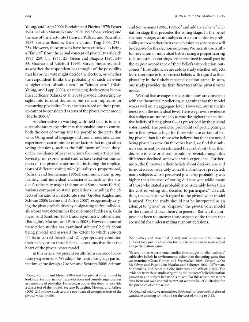
FIGURE 1 Average Subjective Decisiveness Probabilities acrossRounds by Session

0

0.1

0.2

0.3

0.4

0.5

0.6

1 2 3 4 5 6 7 8 9 10 11 12 13 14 15 16 17 18 19 20

Session 1 Session 2 Session 3 Session 4: simple

comprehension of the decisiveness rules and payoff possi-bilities in the belief treatment. They earned slightly moreon average ($15.75) than subjects in the control treatment,but the differences are easily accounted for by the addi-tional payments subjects received for the accuracy of theirbeliefs.

Our main interest in the belief elicitation treatmentis to assess whether subjects vote when their decisivenessbeliefs exceed the cost of voting, p > c = 0.18, and ab-stain otherwise. We are also interested in whether subjectslearn over time to adjust their beliefs toward the actualfrequency of decisiveness.

Results

We report results from seven sessions—four belief elici-tation (or treatment) sessions and three control sessions.Each session involved 20 subjects who made decisions in20 rounds. Thus, there are 1,600 participation (or vot-ing) decisions from the belief elicitation treatment and1,200 from the control treatment, i.e., a total of 2,800 de-cisions. We begin with a discussion of whether changinginstructions in the belief elicitation sessions altered sub-jects’ behavior. This is followed by a brief review of ag-gregate results. The lengthiest part of the results section isdevoted to the primary concern of this article—analyzingthe individual-level behavior. Finally, we test the obtru-siveness of the belief elicitation procedure.

Simple versus Complex Instructions

Figure 1 shows the average subjective decisiveness prob-ability over all 20 rounds of the four belief elicitationsessions. If the more complex instructions systematicallycause overestimation of the probability of being pivotalwhile simple instructions help avoid it, the series for thesingle session with simple instructions (session 4, repre-sented by a black solid line) should stand apart from thelines representing sessions 1–3. However, this is not thecase—the average subjective decisiveness probabilities insession 4 are very similar to those found in the other threesessions. Indeed, when looking at the rest of the graphsthat present information by session and are discussed be-low (Figures 3–6), session 4 does not differ much fromsessions 1–3. Including or excluding information fromthis session in the probit estimations (see Table 2) pro-duces substantively very similar results. Given this, wecan be rather confident that subjects’ ability to estimatetheir pivot probabilities does not depend significantly onthe complexity of instructions.11

11As the next section explains, the aggregate turnout in session 4is higher than that in the other six sessions (see Figure 2). How-ever, given that the turnout rate from session 4 represents a singlecase, it is hard to say whether this difference is systematic. If severaladditional sessions were run with simpler instructions, the averageturnout across those sessions may still look similar to the averageturnout from sessions with complex instructions. For our purposes,more important than the aggregate turnout is the original concernthat complex instructions may introduce a bias into subjects’ es-timations of their pivot probabilities. The latter, however, appearsnot to be the case.


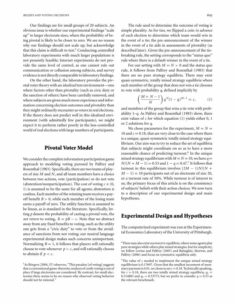
FIGURE 2 Turnout Rates for All Sessions, Five-Round Averages

0

10

20

30

40

50

60

70

1-5 6-10 11-15 16-20

Rounds

Turn

out (

%)

Beliefs 1 Beliefs 2 Beliefs 3 Beliefs 4

No beliefs 1 No beliefs 2 No beliefs 3

Aggregate Results

Figure 2 summarizes turnout using 5-round averages foreach of the seven sessions, labeled beliefs or no-beliefssessions 1, 2, 3, 4. The average turnout in rounds 1–5 isclose to the theoretical prediction of 53%. However, inall sessions, except beliefs session 4, the turnout levelsdrop below 50% over time.12 The differences in turnoutbetween the two treatments are not large. Using data on 5-round averages as shown in Figure 1, and a nonparametricMann-Whitney test, the null hypothesis of no differencein turnout rates between treatments can be rejected onlyin rounds 15–20 at the 0.05 level of significance. On the

12Although this is not an entirely fair comparison given the dif-ferences in experimental design and theoretical predictions, otherexperimental studies of turnout or participation games in general,report participation levels similar to ours. For example, Schram andSonnemans (1996b) use groups of 12 subjects to study turnout un-der different conditions. They do not give a theoretical predictionfor aggregate turnout levels but report observed turnout of about40%. (They use graphs rather than precise numbers to present ag-gregate turnout.) Großer et al. (2005) also use 12 subject groupsand present graphs that report turnout levels of about 40–45%.Bornstein, Kugler, and Zamir (2005) use six subject groups and re-port average turnout of about 55%. Levine and Palfrey (2007) usegroups of varying size and, unlike our study, an unequal number ofplayers in each team. They report turnout levels of about 37% forsessions involving 27 or more subjects (the closest possible compar-ison to our 20-subject design). Similarly to our study, Levine andPalfrey observe turnout levels that are lower than theoretically pre-dicted. However, Goeree and Holt (2005) have shown that for thetype of binary choice games such as ours, observed participationrates tend, in general, to be lower than the theoretical prediction ifthat prediction is above 0.5, which is the case in our study.

other hand, when the data are not grouped into 5-roundaverages, a Mann-Whitney test suggests that the overallaverage turnout rate (all rounds) is significantly higher(at the 0.05 level) for the four beliefs sessions (47%) thanfor the three no-beliefs sessions (39%). The latter findingis attributable to several factors, including the big drop-off in turnout in the no-beliefs sessions toward the end ofthose sessions; the high average turnout—56% (the clos-est to the theoretical prediction)—in beliefs session 4; andfinally the fact that in no-beliefs session 2, one group be-came dominant, i.e., the same group won nearly everyround, thus lowering participation rates in that session.The fraction of decisive games was very similar acrosstreatments: in the beliefs sessions, 21 out of the 80 (14 outof 60 if beliefs session 4 is excluded) games resulted in adecisive participation, while in the control treatment theratio was 12 out of 60. These aggregate findings do notallow us to draw strong conclusions about whether be-lief elicitation affected subjects’ behavior. We will returnto the issue of the potential obtrusiveness of the experi-mental treatment below. To foreshadow the conclusion,we find no significant differences in individual-choice be-havior across treatments, suggesting the belief elicitationprocedure was not obtrusive.

Individual-Level Results

The crucial independent variable in this study is thesubjective decisiveness probability. Subjects could state aprobability with an accuracy of up to three decimal places.


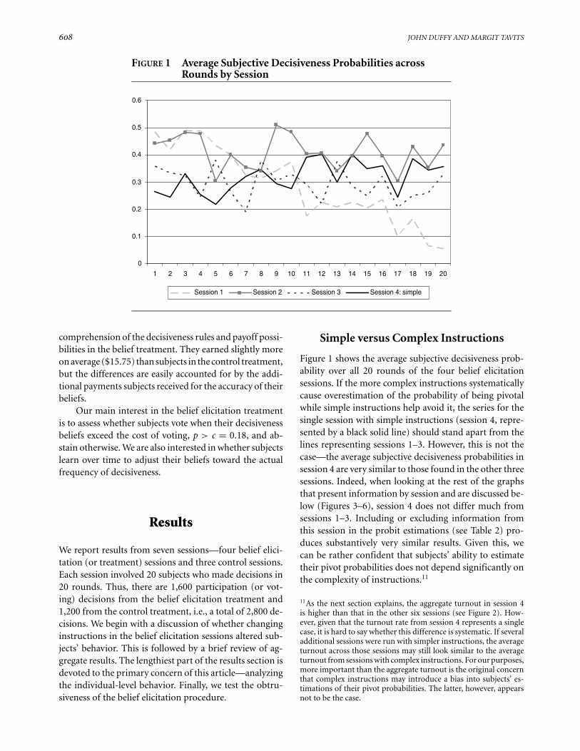
FIGURE 3 Average Frequency Distribution of Subjective Decisiveness Probabilities over TenRounds by Sessions

Session 1

0%10%20%30%40%50%60%70%80%90%

100%

0-.199 .2-.399 .4-.599 .6-.799 .8-1

Period 1-10 Period 11-20

Session 3

0%10%20%30%40%50%60%70%80%90%

100%

0-.199 .2-.399 .4-.599 .6-.799 .8-1


Session 2

0%10%20%30%40%50%60%70%80%90%

100%

0-.199 .2-.399 .4-.599 .6-.799 .8-1


Session 4: s im ple

0%

10%

20%

30%

40%50%

60%

70%

80%

90%

100%

0-.199 .2-.399 .4-.599 .6-.799 .8-1


In all sessions, 0 and 0.5 were modal values, though manyother values were chosen. The mean subjective probabil-ity that an individual is decisive is rather high: 0.33. Itvaries slightly by session, equal to 0.29 for the first andthe third beliefs sessions, 0.41 for the second, and 0.32 forthe fourth.

Figure 3 shows frequency distributions for the sub-jective decisiveness probabilities by session averaged overthe first and last 10 rounds. As the graphs illustrate, sub-jects’ decisiveness probabilities in the first 10 rounds arespread more uniformly over the interval [0,1] than thelast 10 rounds, where the distribution is more skewed tothe left of the interval.

On average, 63% of subjects across all four belief elic-itation sessions stated a probability of being decisive thatwas higher than 0.18. Recall that c = 0.18; thus, the deci-siveness probability of 0.18 serves as the theoretical cut-point for participation. These subjective probabilities ofbeing decisive can be compared to the actual probabil-ities, or the frequencies of past decisiveness. The actualmean frequency of decisiveness (all 20 rounds) averagesout to be 0.149 across all four beliefs sessions. This aver-age frequency is 0.05, 0.21, 0.13, and 0.21 for each session1 through 4, respectively.13 The difference between the

13In the mixed strategy equilibrium, the frequency of decisivenesswould average 0.18.

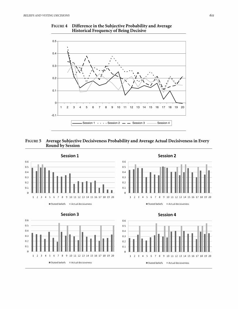
historical average objective frequency of decisiveness andthe subjective frequency of decisiveness is rather substan-tial. Figure 4 illustrates this difference by session; noticethat the difference is always positive, but decreases withexperience.14 The convergence is especially visible in thecase of the first session (solid line) where in the last tworounds the objective and average subjective probabilitiesare equal. This suggests that individuals can learn overtime to adjust their subjective probabilities of decisive-ness in response to histories of voting outcomes in thedirection of the true ex post frequency of decisiveness.The positive values of the series in Figure 4 indicate thatsubjects are almost without an exception overestimatingthe probability.

Figure 5 compares average subjective decisivenesswith the average actual decisiveness in each round of asession. It appears that subjects condition their beliefs ontheir actual experience of being decisive. Consider ses-sion 1: Here, actual decisiveness is a rare event that occursonly twice early in the session and subjects’ stated beliefs

14The average historical decisiveness at the start of round t is theaverage frequency with which subjects have been decisive in allprior rounds t = 1, . . ., t−1. Figure 4 plots the average differencebetween subjects’ stated subjective probability of decisiveness forround t and the average historical decisiveness at the start of round t ,beginning with the second round, as average historical decisivenesscannot be ascertained prior to that round.


FIGURE 4 Difference in the Subjective Probability and AverageHistorical Frequency of Being Decisive

-0.1

0

0.1

0.2

0.3

0.4

0.5

1 2 3 4 5 6 7 8 9 10 11 12 13 14 15 16 17 18 19 20

Session 1 Session 2 Session 3 Session 4

FIGURE 5 Average Subjective Decisiveness Probability and Average Actual Decisiveness in EveryRound by Session


of being decisive decline correspondingly over time. Inother sessions, especially in sessions 2 and 4, actual de-cisiveness occurs more frequently throughout the dura-tion of the session. This helps sustain subjects’ beliefs thatthey may be decisive at relatively high levels through all20 rounds. As above, we can observe that subjects usethe historical frequency of actual decisiveness to formtheir subjective beliefs about the probability of beingdecisive.

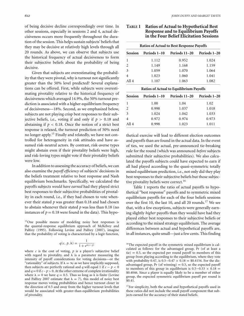
Given that subjects are overestimating the probabil-ity that they were pivotal, why is turnout not significantlygreater than the 50% level predicted? Several explana-tions can be offered. First, while subjects were overesti-mating pivotality relative to the historical frequency ofdecisiveness which averaged 14.9%, the 50% turnout pre-diction is associated with a higher equilibrium frequencyof decisiveness—18%. Second, as we emphasized below,subjects are not playing crisp best responses to their sub-jective beliefs, i.e., voting if and only if p > 0.18 andabstaining if p < 0.18. Once the notion of a strict bestresponse is relaxed, the turnout prediction of 50% needno longer apply.15 Finally and relatedly, we have not con-trolled for heterogeneity in risk attitudes and have as-sumed risk-neutral actors. By contrast, risk-averse typesmight abstain even if their pivotality beliefs were high,and risk-loving types might vote if their pivotality beliefswere low.

In addition to assessing the accuracy of beliefs, we canalso examine the payoff efficiency of subjects’ decisions inthe beliefs treatment relative to best response and Nashequilibrium benchmarks. Specifically, we calculated thepayoffs subjects would have earned had they played strictbest responses to their subjective probabilities of pivotal-ity in each round, i.e., if they had chosen to vote when-ever their stated p was greater than 0.18 and had chosento abstain whenever their stated p was less than 0.18 (noinstances of p = 0.18 were found in the data). This hypo-

15One possible means of modeling noisy best responses isthe quantal-response equilibrium approach of McKelvey andPalfrey (1995). Following Levine and Palfrey (2007), imaginethat the probability of voting is characterized by a logit function,

q(c , p, �) = 1

1 + e�(c−p)

where c is the cost of voting, p is a player’s subjective beliefwith regard to pivotality, and � is a parameter measuring theintensity of payoff considerations for voting decisions—or the“rationality” of subjects. If � = ∞ as we have implicitly supposed,then subjects are perfectly rational and q will equal 1 if c − p < 0and q = 0 if c – p > 0. At the other extreme of complete irrationalitywhere � = 0 we have q = 0.5. Thus so long as � is finite (Levineand Palfrey 2007 estimate that � = 7), this model of noisy bestresponse moves voting probabilities and hence turnout closer inthe direction of 0.5 and away from the higher turnout levels thatwould be associated with greater-than-equilibrium probabilitiesof pivotality.

TABLE 1 Ratios of Actual to Hypothetical BestResponse and to Equilibrium Payoffsin the Four Belief Elicitation Sessions

Ratios of Actual to Best Response Payoffs

Session Periods 1–10 Periods 11–20 Periods 1–20

1 1.112 0.952 1.0242 1.149 1.168 1.1593 1.059 1.070 1.0644 1.023 1.060 1.041All 4 1.107 1.063 1.082

Ratios of Actual to Equilibrium Payoffs

Session Periods 1–10 Periods 11–20 Periods 1–20

1 1.00 1.04 1.022 0.998 1.037 1.0183 1.024 1.042 1.0334 0.972 0.974 0.973All 4 0.998 1.023 1.011

thetical exercise will lead to different election outcomesand payoffs than are found in the actual data. In the eventof ties, we used the actual, pre-announced tie-breakingrule for the round (which was announced before subjectssubmitted their subjective probabilities). We also calcu-lated the payoffs subjects could have expected to earn ifall had played according to the quasi-symmetric totallymixed equilibrium prediction, i.e., not only did they playbest responses to their subjective beliefs but those subjec-tive pivotality beliefs were correct.16

Table 1 reports the ratio of actual payoffs to hypo-thetical “best response” payoffs and to symmetric mixedequilibrium payoffs for each of the four beliefs sessionsover the first 10, the last 10, and all 20 rounds.17 We seethat, with a few exceptions, subjects were generally earn-ing slightly higher payoffs than they would have had theyplayed either best responses to their subjective beliefs oraccording to the mixed strategy equilibrium. The averagedifferences between actual and hypothetical payoffs are,in all instances, quite small—just a few cents. This finding

16The expected payoff in the symmetric mixed equilibrium is cal-culated as follows: for the advantaged group, Pr (of at least atie) = 0.5, so the expected per round payoff to members of thisgroup from playing according to the equilibrium, where they votewith probability 0.47, is 0.5−0.47 × 0.18 = $0.4154. For the dis-advantaged group, Pr (of winning) = 0.5, so the expected payoffto members of this group in equilibrium is 0.5−0.53 × 0.18 =$0.4046. Since a player is equally likely to be a member of eithergroup, the expected symmetric equilibrium payoff per round is$0.41.

17For simplicity, both the actual and hypothetical payoffs used inthese ratios did not include the small payoff component that sub-jects earned for the accuracy of their stated beliefs.


suggests that, while subjects were not playing crisp bestresponses to their stated beliefs (more on this below), norwere their beliefs of pivotality consistent with the equilib-rium prediction, they nevertheless appear to have been noworse off as the result, so their incentives to move furthertoward the rational choice, equilibrium prediction mayhave been weak.

Multivariate Analyses

In order to further understand the effect of subjectivebeliefs of pivotality on the likelihood of buying a token,we have conducted a number of multivariate probit re-gressions. As individual decisions within sessions are notentirely independent, we have clustered the standard er-rors on subjects in all analyses. The results are presentedin Table 2. Model 1 estimates the effect of the stated be-liefs of being pivotal (continuous variable) on the deci-sion to vote (binary variable) while Model 2 replicatesthe same analysis using a dummy variable coded “1” forthose who stated a probability of being pivotal higherthan 0.18 in order to test the exact predictions of thetheory.

Both models include several controls. First, we con-trol for whether the group of which the subject is a mem-ber will win in the event of a tie. This variable might alsobe thought of as proxying for a preelection poll announc-ing a lead to one candidate. The pivotal voter model pre-dicts lower turnout for the “advantaged” group (see fn.7; Levine and Palfrey 2007). Further, since we ran sev-eral rounds of “elections” and the group members stayedthe same across rounds, we also control for various his-tory effects. These include (1) whether a given subjectwas pivotal in the last round, (2) whether the subjectbought a token in the last round, (3) whether the sub-ject’s group won the last round, (4) the number of tokensbought by the subject’s group in the last round, (5) thesubject’s earnings from the last round, and (6) whetherthere was a tie in the last round. We also control for ses-sion effects using session dummies and for the roundnumber.

The results of Model 1 show a strong effect of thestated probability of being decisive on the probability ofbuying a token. Substantively, the predicted probabilityof buying a token is 0.15 when the stated probability ofbeing pivotal is 0 (i.e., at its minimum) and 0.34 when it is1 (at its maximum), holding other variables at their mean(for continuous variables) or median (for categorical vari-ables; session dummies are held at 0). Model 2 producessimilar results—the predicted probability for buying a to-ken is 0.15 when the stated probability of being pivotal is

higher than 0.18 and only slightly higher, 0.26, when itis lower than 0.18, all other variables at their mean ormedian.18

These results suggest that the subjective probabilityof being pivotal plays a significant role in people’s deci-sion to participate: the higher the subjective probabilitythe greater the likelihood of buying a token. The resultsare not, however, as crisp as the theory would predict:a subjective probability of 0.18 does not function as aclear cutpoint for the decision to participate. If subjectswere playing according to the crisp cutpoint predictionof the theory, those who stated a probability of beingpivotal greater than or equal to 0.18 should participate,while those who stated a lower probability should ab-stain. However, only 52% of the former participated and60% of the latter abstained. Further, although the deci-siveness probabilities of participants are usually higherthan those of nonparticipants, there does not appear tobe a clear average cutpoint for participation. Thus, thereis only weak support for the specific prediction of the the-ory. Few participants use the exact deterministic cutpointstrategy predicted by the theory. However, there is evi-dence that subjects’ behavior tends toward the theoreticalprediction with higher subjective probabilities increasingthe likelihood of participation. Furthermore, as discussedabove, subjects’ payoff efficiency is already approximatelyequal to that of a rational choice voter.

Additional Findings

In addition to the main findings, some of the variablesmeasuring the effects of history or past behavior are alsosignificantly related to the decision to participate. First,round number or trend has a significant negative effecton the probability of buying a token: all else equal, sub-jects were less likely to buy a token in later than in earlierrounds. This may indicate a certain learning effect in termsof cumulative disappointment in low payoffs from buy-ing a token, or the emergence of a free rider problem (seeBendor, Diermeier, and Ting 2003; Kanazawa 2000 for

18We also estimated models that included the average historical fre-quency of being decisive in addition to the other variables reportedin Table 2, Models 1 and 2. This did not diminish the effect ofthe subjective probabilities of being decisive. Rather, the objectivefrequencies had a negative and no statistically significant effect onturnout while the effect of subjective beliefs remained significantand in the predicted direction. This underlines the importance ofsubjective beliefs of being pivotal in turnout decisions and chal-lenges the use of some objective measures of this probability, suchas closeness of an election, when testing the pivotal voter model.As we saw, although over time the subjective probability of beingpivotal tends toward the actual frequency, the differences can besubstantial.


TABLE 2 Probit Models of the Effect of Subjective Decisiveness Probability on Turnout

Model 1: Model 2: Model 3: Model 4:beliefs beliefs no-beliefs all sessionsb(SE) b(SE) b(SE) b(SE)

Beliefs elicited 0.151

(0.187)Subjective Pr(Decisive) 0.615∗∗∗

(0.184)Subjective Pr(Decisive) >0.18 0.389∗∗∗

(0.116)Historical frequency of decisiveness 1.219 −0.024

(0.935) (0.386)Group wins tie 0.231∗∗ 0.239∗∗ 0.549∗∗ 0.365∗∗∗

(0.111) (0.113) (0.129) (0.079)Decisive t − 1 0.153 0.164 0.218 0.257∗∗∗

(0.124) (0.128) (0.143) (0.099)Participate t − 1 1.011∗∗∗ 0.995∗∗∗ 0.861∗∗ 0.912∗∗∗

(0.132) (0.123) (0.152) (0.102)Win t − 1# −0.010 −0.012 0.075

(0.083) (0.083) (0.082)Number of group tokens t − 1 −0.109∗∗∗ −0.107∗∗∗ −0.112∗∗ −0.105∗∗∗

(0.025) (0.025) (0.026) (0.019)Earnings t − 1 0.042 0.018 0.322∗∗ 0.077

(0.110) (0.109) (0.142) (0.085)Tie t − 1 −0.041 −0.018 0.581∗∗ 0.084

(0.127) (0.130) (0.185) (0.103)Round (trend) −0.008∗ −0.007 −0.044∗∗ −0.023∗∗∗

(0.005) (0.005) (0.007) (0.004)Beliefs session 2 0.091 0.041 −0.009

(0.240) (0.234) (0.183)Beliefs session 3 0.203 0.156 −0.107

(0.322) (0.322) (0.191)Beliefs session 4 0.738∗∗ 0.657∗ 0.277

(0.377) (0.377) (0.219)No-beliefs session 2 0.147 0.158

(0.181) (0.135)No-beliefs session 3 −0.071 −0.075

(0.177) (0.163)Constant −0.320∗ −0.348∗ −0.341∗ −0.249∗

(0.190) (0.201) (0.172) (0.132)� 2 279.37∗∗∗ 265.01∗∗∗ 123.56∗∗ 173.28∗∗∗

Pseudo R2 0.12 0.12 0.12 0.11N 1520 1520 1140 2660

Note: Table entries are probit coefficients with robust standard errors, clustered on subject, in parentheses. Dependent variable is whetheror not a token was bought. ∗p≤0.1, ∗∗p≤0.05, ∗∗p≤0.01 #In Model 3, Win t − 1 is dropped due to colinearity.

learning effects). This result also reflects the observationthat turnout declines when democracies mature, i.e., as aresult of repeated elections (Kostadinova 2003). Second,subjects are more likely to participate when they have par-

ticipated before. This result reflects the argument aboutthe “habitual voter” (Gerber, Green, and Shachar 2003;Plutzer 2002) made in a previous empirical literature onturnout.


Further, the participation rate of one’s group mem-bers also significantly influences an individual’s decisionto buy a token: a subject is less likely to participate if thegeneral participation rate in his or her group was high,indicating the emergence of a free rider problem. Priorhigh participation rate in one’s own group may generateexpectations of a similarly high participation level in thesubsequent round. Given such an expectation, it is ratio-nal for a subject to abstain and avoid the cost of votingyet still expect to benefit from one’s group winning. In-terestingly, our result contradicts the argument that insituations that require voluntary contributing to publicgoods, conditional cooperation or reciprocity is the beststrategy for each player (Axelrod 1984). Our experiment,however, is not only limited to such intragroup conflictbut also includes intergroup conflict, which may explainwhy conditional cooperation does not occur. Past groupsuccess or failure does not play a significant role in deci-sions to participate.

Models 1 and 2 also allow us to test a further im-plication of the theory. Recall that in the unique quasi-symmetric mixed strategy equilibrium the turnout prob-abilities for the two groups are not the same (see fn. 7).Rather, we predicted an underdog effect (Levine and Pal-frey 2007), where the group winning a tie should havehigher turnout than the disadvantaged group. The Groupwins tie variable in Models 1 and 2 captures this relation-ship. Contrary to the theory, the finding indicates thatthe tie-breaking rule acts as a coordination device for vot-

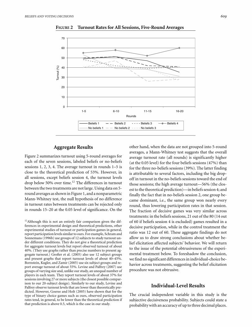
FIGURE 6 Turnout in Advantaged and Disadvantaged Groups

0

10

20

30

40

50

60

70

Beliefs 1 Beliefs 2 Beliefs 3 Beliefs 4 No-beliefs 1 No-beliefs 2 No-beliefs 3

Turn

ou

t (%

)

Advantaged group Disadvantaged group

0

10

20

30

40

50

60

70

Beliefs 1 Beliefs 2 Beliefs 3 Beliefs 4 No-beliefs 1 No-beliefs 2 No-beliefs 3

Turn

ou

t (%

)

Advantaged group Disadvantaged group

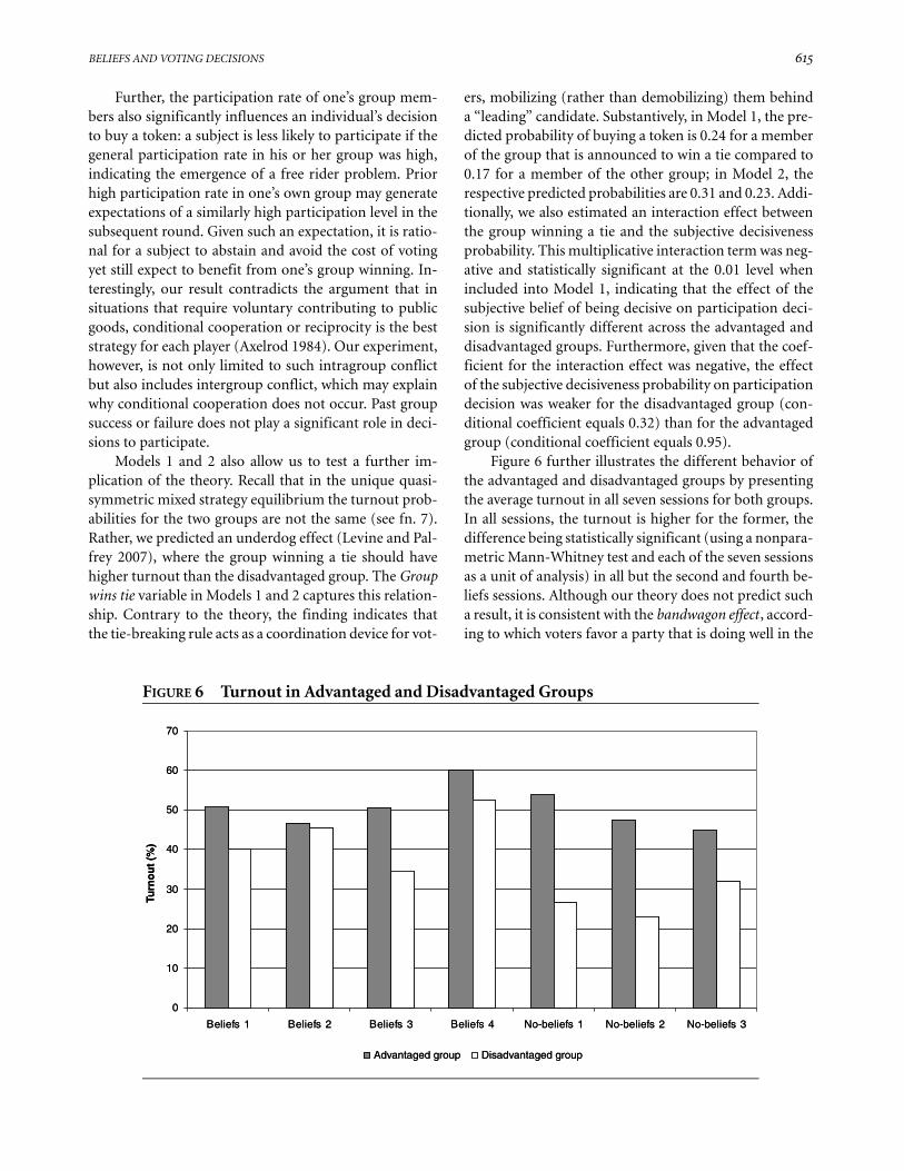
ers, mobilizing (rather than demobilizing) them behinda “leading” candidate. Substantively, in Model 1, the pre-dicted probability of buying a token is 0.24 for a memberof the group that is announced to win a tie compared to0.17 for a member of the other group; in Model 2, therespective predicted probabilities are 0.31 and 0.23. Addi-tionally, we also estimated an interaction effect betweenthe group winning a tie and the subjective decisivenessprobability. This multiplicative interaction term was neg-ative and statistically significant at the 0.01 level whenincluded into Model 1, indicating that the effect of thesubjective belief of being decisive on participation deci-sion is significantly different across the advantaged anddisadvantaged groups. Furthermore, given that the coef-ficient for the interaction effect was negative, the effectof the subjective decisiveness probability on participationdecision was weaker for the disadvantaged group (con-ditional coefficient equals 0.32) than for the advantagedgroup (conditional coefficient equals 0.95).

Figure 6 further illustrates the different behavior ofthe advantaged and disadvantaged groups by presentingthe average turnout in all seven sessions for both groups.In all sessions, the turnout is higher for the former, thedifference being statistically significant (using a nonpara-metric Mann-Whitney test and each of the seven sessionsas a unit of analysis) in all but the second and fourth be-liefs sessions. Although our theory does not predict sucha result, it is consistent with the bandwagon effect , accord-ing to which voters favor a party that is doing well in the


polls, reported in several voting studies (McAllister andStudlar 1991). Here, this finding may have occurred asan artifact of our particular experimental design, i.e., theuse of ex ante coin toss (or status quo) rule for break-ing ties and fixed group membership. An alternative, yetstrategically equivalent design might declare in advancethat one group always wins a tie and employ random re-matching of subjects into groups as opposed to our fixedgroup membership design. If the bandwagon effect dis-appears, then we might attribute the current result to ourdesign.19

Testing the Obtrusiveness of the BeliefElicitation Procedure

Models 3 and 4 in Table 2 replicate Model 1 with data fromthe control treatment and from all sessions respectively,using historical frequency of decisiveness instead of thestated beliefs of being pivotal. The goal here is to deter-mine whether subjects behaved significantly differentlywhen beliefs were elicited compared to the control group.Most importantly, the dummy variable differentiating be-tween treatment and control sessions (variable name Be-liefs elicited) in Model 4 is not statistically significant. Thisallows us to conclude that there are no significant differ-ences in the behavior of subjects across treatments andthat our belief elicitation procedure was not obtrusive interms of making subjects more aware of the rationality ofparticipating.

Furthermore, Model 3 produces roughly similar re-sults as Model 1. As above, we find that the tie-breakingrule influences turnout, prior participation increaseswhile high level of group participation depresses the like-lihood of current participation, and turnout decreasessignificantly over time. Further, as above (see fn. 18), theeffect of the historical frequency of decisiveness falls shortof the conventional level of statistical significance. Thesesimilarities across treatments further suggest that the be-lief elicitation was unobtrusive in terms of influencingsubjects’ decision making.

There are also some differences, however: both priorearnings and history of ties significantly and positivelyinfluence turnout. These history effects are likely influ-encing one’s subjective probability of being pivotal, and

19Interestingly, a recent study presents the results of an experimen-tal participation game with random rematching design withouteliciting beliefs and reports a similar bandwagon effect (Bornstein,Kugler, and Zamir 2005). When beliefs are elicited, a random re-matching design might make it more difficult for subjects to assessor adjust their subjective probability of decisiveness. We leave thisexercise to future research.

as such, may reflect some of the effects otherwise capturedby the subjective beliefs.

Conclusions

The pivotal voter model that builds on Downs’ (1957)rational choice theory of turnout is the most intuitive,yet also the most controversial formal theory in politicalscience. Empirical tests of the theory to date have mostlyrelied on proxies or have been partial. The concept aroundwhich much of the controversy revolves—the probabilityof being pivotal—has received the least empirical atten-tion. Indeed, pivotality is simply inferred from the close-ness of the election, and the individual-level calculus ofvoting is never unpacked.

This study has provided the first direct test of thepivotal voter model, with a specific focus on whether andhow voters’ beliefs of being pivotal factor into their votingdecisions. We used a context-free laboratory setting thatallows us to control voting benefits and costs and to elicitvoters’ beliefs about pivotality.

On the aggregate level, we find support for the pivotalvoter model with aggregate turnout rates that are close,though slightly below theoretical predictions. The mainfocus of this study, however, is on the individual-level be-havior, where we find mixed support for the theory. On theone hand, we find that subjects’ beliefs do inform us as totheir likely voting decision. Subjects who believe that theirparticipation will be pivotal for the outcome of a game (anelection) are more likely to participate. This relationshipis strong and robust, but it is not deterministic—there isno single cutpoint strategy of participation that applies toall voters as predicted by the theory. On the other hand, wehave found that subjects systematically overestimate theprobability that their voting decision will be pivotal. Theweakness in the empirical support for the theory comesnot from the failure of subjects to best respond to theirbeliefs; rather, it comes from the failure of subjects tohold the correct beliefs in the first place, a distinction thatcould not have been understood prior to conducting thisexperiment.

Additionally, we have found that subjective beliefsare more important for the participation (turnout) deci-sion than the actual frequencies of being decisive. Indeed,the subjective probabilities tend to be considerably higherthan the actual ones—undermining the common viewthat closeness is a useful proxy for pivotality in testingrational models of turnout. Yet, we also find that, on av-erage, beliefs become somewhat more accurate over time,indicating a learning effect in the turnout decision. The


overestimation of pivotality may, thus, provide a solutionto the paradox of voter turnout—voting happens becausepeople systematically think that their vote counts morethan it actually does, though this overestimation declineswith experience.

References

Aldrich, John H. 1993. “Rational Choice and Turnout.” Ameri-can Journal of Political Science 37(1): 246–78.

Axelrod, Robert. 1984. The Evolution of Cooperation. New York:Basic Books.

Battaglini, Marco, Rebecca Morton, and Thomas Palfrey. 2006.“The Swing Voter’s Curse in the Laboratory.” Working Paper.Princeton University, California Institute of Technology, andNew York University.

Bendor, Jonathan, Daniel Diermeier, and Michael Ting. 2003.“A Behavioral Model of Turnout.” American Political ScienceReview 97(2): 261–80.

Blais, Andre, and Robert Young. 1999. “Why Do People Vote?An Experiment in Rationality.” Public Choice 99(1–2): 39–55.

Blais, Andre, Robert Young, and Miriam Lapp. 2000. “The Cal-culus of Voting: An Empirical Test.” European Journal of Po-litical Research 37(2): 181–201.

Borgers, Tilman. 2004. “Costly Voting.” American Economic Re-view 94: 57–66.

Bornstein, Gary, Tamar Kugler, and Shmuel Zamir. 2005. “OneTeam Must Win, the Other Need Only Not Lose: An Ex-perimental Study of an Asymmetric Participation Game.”Journal of Behavioral Decision Making 18(2): 111–23.

Brier, Glenn W. 1950. “Verification of Forecasts Expressed inTerms of Probability.” Monthly Weather Review 78(1): 1–3.

Camerer, Colin. 1995. “Individual Decision Making.” In TheHandbook of Experimental Economics, ed. John H. Kagel andAlvin E. Roth. Princeton, NJ:Princeton University Press, 587–703.

Clarke, Harold D., David Sanders, Marianne C. Stewart, andPaul F. Whiteley. 2004. Political Choice in Britain. Oxford:Oxford University Press.

Coate, Stephen, Michael Conlin, and Andrea Moro. 2004. “ThePerformance of the Pivotal-Voter Model in Small-Scale Elec-tions: Evidence from Texas Liquor Referenda.” Unpublishedmanuscript. Cornell University.

Costa-Gomes, Miguel A., and Georg Weizsacker. 2005. “StatedBeliefs and Play in Normal Form Games.” Unpublishedmanuscript. London School of Economics and PoliticalScience.

Croson, Rachel T. A. 2000. “Thinking Like a Game Theorist:Factors Affecting the Frequency of Equilibrium Play.” Jour-nal of Economic Behavior and Organization 41(3): 299–314.

Cyr, A. Bruce. 1975. “The Calculus of Voting Reconsidered.”Public Opinion Quarterly 39(1): 19–38.

Dhillon, Amrita, and Susana Peralta. 2002. “Economic Theoriesof Voter Turnout.” Economic Journal 112: F332–F352.

Downs, Anthony. 1957. An Economic Theory of Democracy. NewYork: Harper & Row.

Feddersen, Timothy, Sean Gailmard, and Alvaro Sandroni. 2007.“Moral Bias in Large Elections: Theory and Experimental Ev-idence.” Unpublished manuscript. Northwestern University.

Ferejohn, John, and Morris P. Fiorina. 1975. “Closeness CountsOnly in Horseshoes and Dancing.” American Political ScienceReview 69(3): 920–25.

Foster, Carroll B. 1984. “The Performance of Rational VoterModels in Recent Presidential Elections.” American PoliticalScience Review 78(3): 678–90.

Friedman, Jeffrey, ed. 1995. The Rational Choice Controversy.New Haven, CT: Yale University Press.

Gerber, Alan S., Donald P. Green, and Ron Shachar. 2003.“Voting May Be Habit-Forming: Evidence from a Random-ized Field Experiment.” American Journal of Political Science47(3): 540–50.

Goeree, Jacob, and Charles Holt. 2005. “An Explanation ofAnomalous Behavior in Models of Political Participation.”American Political Science Review 99(2): 201–13.

Green, Donald P., and Ian Shapiro. 1994. Pathologies of RationalChoice Theory. New Haven, CT: Yale University Press.

Großer, Jens, Tamar Kugler, and Arthur Schram. 2005. “Pref-erence Uncertainty, Voter Participation and Electoral Effi-ciency: An Experimental Study.” Unpublished manuscript.University of Cologne.

Großer, Jens, and Arthur Schram. 2006. “Neighborhood Infor-mation Exchange and Voter Participation: An ExperimentalStudy.” American Political Science Review 100(2): 235–48.

Hansen, Steven, Thomas Palfrey, and Howard Rosenthal. 1987.“The Relationship between Constituency Size and Turnout:Using Game Theory to Estimate the Cost of Voting.” PublicChoice 52(1): 15–33.

Kanazawa, Satoshi. 2000. “A New Solution to the CollectiveAction Problem: The Paradox of Voter Turnout.” AmericanSociological Review 65(3): 433–42.

Kostadinova, Tatiana. 2003. “Voter Turnout Dynamics in Post-Communist Europe.” European Journal of Political Research42(6): 741–59.

Ledyard, John O. 1984. “The Pure Theory of Large Two-Candidate Elections.” Public Choice 52(1): 15–33.

Levine, David K., and Thomas R. Palfrey. 2007. “The Paradox ofVoter Participation? A Laboratory Study.” American PoliticalScience Review 101(1): 143–58.

Matsusaka, John G., and Filip Palda. 1993. “The DownsianVoter Meets the Ecological Fallacy.” Public Choice 77(4): 855–78.

McAllister, Ian, and Donley T. Studlar. 1991. “Bandwagon, Un-derdog, or Projection? Opinion Polls and Electoral Choicein Britain, 1979–1987.” Journal of Politics 53(3): 720–41.

McKelvey, Richard D., and Talbot Page. 1990. “Public and Pri-vate Information: An Experimental Study of InformationPooling.” Econometrica 58(6): 1321–39.

McKelvey, Richard D., and Thomas R. Palfrey. 1995. “QuantalResponse Equilibria for Normal Form Games.” Games andEconomic Behavior 10(1): 6–38.

Merlo, Antonio. 2006. “Whither Political Economy? Theories,Facts and Issues.” In Advances in Economics and Economet-rics: Theory and Applications, Ninth World Congress, Vol-ume 1 (Econometric Society Monographs no. 41), ed. R.Blundell et al. Cambridge: Cambridge University Press, 381–421.


Nyarko, Yaw, and Andrew Schotter. 2002. “An ExperimentalStudy of Belief Learning Using Elicited Beliefs.” Econometrica70(3): 971–1005.

Offerman, Theo, Joep Sonnemans, and Arthur Schram, 1996.“Value Orientations, Expectations and Voluntary Contribu-tions in Public Goods.” Economic Journal 106: 817–45.

Offerman, Theo, Joep Sonnemans, and Arthur Schram. 2001.“Expectation Formation in Step-Level Public Good Games.”Economic Inquiry 2(2): 250–56.

Palfrey, Thomas R., and Howard Rosenthal. 1983. “A StrategicCalculus of Voting.” Public Choice 41(1): 7–53.

Palfrey, Thomas R., and Howard Rosenthal. 1985. “Voter Partic-ipation and Strategic Uncertainty.” American Political ScienceReview 79(1): 62–78.

Palfrey, Thomas R., and Howard Rosenthal. 1988. “Private In-centives in Social Dilemmas: The Effects of Incomplete In-formation and Altruism.” Journal of Public Economics 35(3):309–32.

Plutzer, Eric. 2002. “Becoming a Habitual Voter: Inertia, Re-sources, and Growth in Young Adulthood.” American Polit-ical Science Review 96(1): 41–56.

Riker, William, and Peter Ordeshook. 1968. “A Theory of theCalculus of Voting.” American Political Science Review 79(1):62–78.

Rutstrom, E. Elisabet, and Nathaniel T. Wilcox. 2004. “Learn-ing and Belief Elicitation: Observer Effects.” Unpublishedmanuscript. University of Houston.

Schram, Arthur, and Joep Sonnemans. 1996a. “Voter Turnoutas a Participation Game: An Experimental Investiga-tion.” International Journal of Game Theory 25(3): 385–406.

Schram, Arthur, and Joep Sonnemans. 1996b. “Why PeopleVote: Experimental Evidence.” Journal of Economic Psychol-ogy 17(4): 417–42.

Shachar, Ron, and Barry Nalebuff. 1999. “Follow the Leader:Theory and Evidence on Political Opinion.” American Eco-nomic Review 89(3): 525–47.

Tullock, Gordon. 1967. Towards the Mathematics of Politics. AnnArbor: University of Michigan Press.

Winkler, R. L., and A. H. Murphy. 1968. “‘Good’ Probabil-ity Assessors.” Journal of Applied Meteorology 7(5): 751–58.

Beliefs and Voting Decisions: A Test of the Pivotal Voter Model

Documents

Transcript of Beliefs and Voting Decisions: A Test of the Pivotal Voter Model