Belgium

Aerodynamic Measurements at Low Reynolds Numbers for Fixed

Wing Micro-Air Vehicles

By

Thomas J. Mueller

to be presented at the

RTO AVT/VKI Special Course on

Development and Operation of UAVs for Military and Civil Applications

September 13-17, 1999VKI, Belgium

Hessert Center for Aerospace ResearchUniversity of Notre Dame

Aerodynamic Measurements at Low Reynolds Numbers

for Fixed Wing Micro-Air Vehicles

Thomas J. MuellerRoth-Gibson Professor

Hessert Center for Aerospace Research

Department of Aerospace and Mechanical Engineering

University of Notre Dame

Notre Dame, IN 46556

USA

Summary

A description of the micro-air vehicle (MAV) con-cept and design requirements is presented. These vehiclesare very small and therefore operate at chord Reynoldsnumbers below where very little data is avail-able on the performance of lifting surfaces, i.e., airfoilsand low aspect-ratio wings. This paper presents the re-sults of a continuing study of the methods that can be usedto obtain reliable force and moment data on thin wings inwind and water tunnels. To this end, a new platform forceand moment balance, similar to an already existing bal-ance, was designed and built to perform lift, drag and mo-ment measurements at low Reynolds numbers. Balancecharacteristics and validation data are presented. Resultsshow a good agreement between published data and dataobtained with the new balance. Results for lift, drag andpitching moment about the quarter chord with the exist-ing aerodynamic balance on a series of thin flat platesand cambered plates at low Reynolds numbers are pre-sented. They show that the cambered plates offer betteraerodynamic characteristics and performance. Moreover,it appears that the trailing-edge geometry of the wingsand the turbulence intensity up to about in the windtunnel do not have a strong effect on the lift and dragfor thin wings at low Reynolds numbers. However, thepresence of two endplates for two-dimensional tests andone endplate for the semi-infinite tests appears to havean undesirable influence on the lift characteristics at lowReynolds numbers. The drag characteristics for thin flat-plate wings of aspect ratio greater than one do not appearto be affected by the endplates. The effect of the endplateson the drag characteristics of cambered-plate wings is stillunder investigation. It is known, however, that endplatesdo have an effect on the drag and lift characteristics of acambered Eppler 61 airfoil/wing.

Copyright co1999 by Thomas J. Mueller. Published by RTO withpermission.

Nomenclature

Symbols

$5 full-span aspect ratio&' drag coefficient (3D)&G section drag coefficient (2D)&/ lift coefficient (3D)&O section lift coefficient (2D)&/m or &Om lift-curve slope

& / &' endurance parameter

&P pitching moment coefficient aboutthe quarter chord

&Pmslope of pitching moment curve

/ ' lift-to-drag ratio0 resolution of A/D converter5HF or 5H root-chord Reynolds number8 freestream velocityD lift-curve slopeD 2D lift-curve slopeE wing spanF root-chord lengthH4 quantization errorV$5 semi-span aspect ratioW wing thicknessm angle of attackm&/ zero-lift angle of attackmVWDOO stall angle of attack~ Glauert parameter

Subscripts

max maximummin minimum

Abbreviations

2D two-dimensional (airfoil)3D three-dimensional (wing)A/D analog-to-digitalTE trailing edgeUND-FB1 old Notre Dame aerodynamic force balanceUND-FB2 new Notre Dame aerodynamic force balance

1

Introduction

There is a serious effort to design aircraft that areas small as possible for special, limited-duration militaryand civil missions. These aircraft, called micro-air ve-hicles (MAVs) (Davis et al, 1996; Ashley, 1998; Wilson1998; Dornheim, 1998; Mraz, 1998; and Fulghum, 1998),are of interest because electronic surveillance and detec-tion sensor equipment can now be miniaturized so thatthe entire payload mass is about 18 grams. The advan-tages of a MAV include compact system transportable bya single operator, rapid deployment, real-time data, lowradar cross-section, difficult to see and very quiet. Thepotential for low production cost is also an advantage.The primary missions of interest for fixed wing MAVsinclude surveillance, detection, communications, and theplacement of unattended sensors. Surveillance missionsinclude video (day and night) and infrared images of bat-tlefields (referred to as the “over the hill” problem) andurban areas (referred to as “around the corner”). Thesereal-time images can give the number and location of op-posing forces. This type of information can also be use-ful in hostage rescue and counter-drug operations. Be-cause of the availability of very small sensors, detectionmissions include the sensing of biological agents, chemi-cal compounds and nuclear materials (i.e., radioactivity).MAVs may also be used to improve communications inurban or other environments where full-time line of sightoperations are important. The placement of acoustic sen-sors on the outside of a building during a hostage rescueor counter-drug operation is another possible mission.

The requirements for fixed wing MAVs cover a widerange of possible operational environments including ur-ban, jungle, desert, maritime, mountains and arctic envi-ronments. Furthermore, MAVs must be able to performtheir missions in all weather conditions (i.e., precipita-tion, wind shear, and gusts). Because these vehicles flyat relatively low altitudes (i.e., less than P) wherebuildings, trees, hills, etc. may be present, a collisionavoidance system is also required.

The long term goal of this project is to develop air-craft systems with a mass of less than 30 grams, haveabout an eight centimeter wing span that can fly for 20to 30 minutes at between 30 and NP KU. The cur-rent goal is to develop aircraft with a 15 centimeter wingspan that have a mass of about 90 grams. The grossmass of micro-air vehicles and other flying objects ver-sus Reynolds number is shown in Figure 1, with the datafrom Jackson (1996-97), Taylor (1969-70), and Tennekes(1996). Since it is not possible to meet all of the designrequirements for a micro-air vehicle with current technol-ogy, research is proceeding on all of the system compo-nents at various government laboratories, companies anduniversities.

Design aims

The design requirements cover a wide range when

1.E-04

1.E-03

1.E-02

1.E-01

1.E+00

1.E+01

1.E+02

1.E+03

1.E+04

1.E+05

1.E+06

1.E+03 1.E+04 1.E+05 1.E+06 1.E+07 1.E+08

Reynolds Number

Ma

ss (

kg)

Butterfly

Pheasant

Cessna 210

B747

MAV

Figure 1: Reynolds number range for flight vehicles

one considers the diversity of possible applications formicro-air vehicles. The MAV must be designed as asystem consisting of airframe, propulsion, payload andavionics. Although much smaller than currently opera-tional UAVs, electrically powered MAVs will have ap-proximately the same weight fractions, that is, forthe airframe, for the engine, for the battery,for the payload, and for avionics and miscellaneousitems. Minimum wing area for ease of packaging andpre-launch handling is also important. Figure 2 presentsthe payload mass versus wingspan for MAVs and otherlarger UAVs.

Figure 2: UAV payload vs wingspan (Davis, 1999)(Reprinted with permission of MIT Lincoln

Laboratory, Lexington, Massachusetts)

A typical fixed wing MAV mission (Morris, 1997)could include the following sequence of events:

1. Launch and climb to 100 meters

2. High speed dash (NP KU Indicated Air Speed) totarget (at NP KU head wind)

2

3. Loiter over target area

4. Maneuver over target during loiter while turning atthe minimum radius

5. Descend and climb over target area

6. Climb to 100 meters

7. High speed dash (NP KU Indicated Air Speed) tolaunch point (tail wind NP KU).

Mission constraints in this simulation include dura-tion, operational radius, minimum turning radius, min-imum climb angle, maximum altitude and number ofclimbs. Several MAV designs have been built and flownwith this type of mission in mind. A FP, square plan-form internal combustion engine powered vehicle calledthe Flyswatter has been flown by Morris (1997). A rudderand elevator surfaces are used to control this MAV. Thefirst electric poweredFP MAV with proportional radiocontrol carrying a video camera was designed and flownby Matthew T. Keennon ofAeroVironment. This vehiclecalled the Black Widow currently holds the record forendurance at 22 minutes (Keennon, 1999). Other MAVswith larger dimensions have been designed and flown tohelp develop the electronic packages and control systems(Harris, 1999; and Ailinger, 1999). Although these areexamples of current vehicles, further improvements willbe made when more data on low Reynolds number aero-dynamics is available and smaller, more efficient electricmotors and propellers have been developed.

The airfoil section and wing planform of the liftingsurface occupy a central position in all design proceduresfor flying vehicles. Therefore, all low Reynolds num-ber vehicles share the ultimate goal of a stable and con-trollable vehicle with maximum aerodynamic efficiency.Aerodynamic efficiency is defined in terms of the lift-to-drag ratio. Airfoil section&OPD[ , &GPLQ

and&O &GPD[

as a function of Reynolds number are shown in Fig-ures 3a, 3b, and 3c after McMasters and Henderson(1980). It is clear from this figure that airfoil perfor-mance deteriorates rapidly as the chord Reynolds num-ber decreases below . While the maximum lift-to-drag ratio for most low-speed fixed-wing aircraft (8 P V) is greater than 10, values for insectsand small birds are usually less than 10. Furthermore, toachieve these values for MAVs at low Reynolds numbers,the wings must emulate bird and insect wings and be verythin (i.e., W F ) with a modest amount of camber.

Requirements for a typical propeller driven MAV,for example, include long flight duration (i.e., high valueof & / &' at speeds up toNP KU at chord Reynoldsnumbers from about to and altitudesfrom 30 to 100 meters). Since these vehicles are es-sentially small flying wings, there is a need to developefficient low Reynolds number, low aspect-ratio wingswhich are not overly sensitive to wind shear, gusts, andthe roughness produced by precipitation. Furthermore,

(a) Maximum lift coefficient

(b) Minimum drag coefficient

(c) Maximum lift-to-drag ratio

Figure 3: Airfoil performance(McMasters and Henderson, 1980)

3

confidence that the operational vehicle will perform asdesigned is important in all applications.

Flow problems

Although design methods developed over the past35 years produce efficient airfoils for chord Reynoldsnumbers greater than about , these methods aregenerally inadequate for chord Reynolds numbers below , especially for very thin airfoils. In relation tothe airfoil boundary layer, important areas of concern arethe separated regions which occur near the leading and/ortrailing edges and transition from laminar to turbulentflow if it occurs. It is well known that separation andtransition are highly sensitive to Reynolds number, pres-sure gradient, and the disturbance environment. Transi-tion and separation play a critical role in determining thedevelopment of the boundary layer which, in turn, affectsthe overall performance of the airfoil. The aerodynamiccharacteristics of the wing and other components in turnaffect the static, dynamic and aeroelastic stability of theentire vehicle. Therefore the successful management ofthe sensitive boundary layer for a particular low Reynoldsnumber vehicle design is critical.

The survey of low Reynolds number airfoils byCarmichael (1981), although almost two decades old, isa very useful starting point in the description of the char-acter of the flow over airfoils over the range of Reynoldsnumbers of interest here. The following discussion offlow regimes from 5HF is a modi-fied version of Carmichael’s original work.

q In the range between 5HF , theboundary layer flow is laminar and it is very difficultto cause transition to turbulent flow. The dragon flyand the house fly are among the insects that fly inthis regime. The dragon fly wing has a sawtoothsingle surface airfoil. It has been speculated thateddies in the troughs help keep the flow from sepa-rating. The house fly wing has large numbers of finehair-like elements projecting normal to the surface.It is speculated that these promote eddy-induced en-ergy transfer to prevent separation. Indoor Mica Filmtype model airplanes also fly in this regime. It hasbeen found that both blunt leading and trailing edgesenhance the aerodynamic performance.

q For chord Reynolds numbers between and , the boundary layer is completely laminarand artificial tripping has not been successful. Ex-perience with hand-launched glider models indicatesthat when the boundary layer separates it does notreattach.

q The range 5HF is of great in-terest to MAV designers as well as model aircraftbuilders. The choice of an airfoil section is very im-portant in this regime since relatively thick airfoils(i.e., and above) can have significant hysteresis

effects caused by laminar separation with transitionto turbulent flow. Also below chord Reynolds num-bers of about , the free shear layer after lami-nar separation normally does not transition to turbu-lent flow in time to reattach. Near the upper end ofthis range, the critical Reynolds number can be de-creased by using boundary layer trips. Thin airfoilsections (i.e., less than thick) at the upper endof this regime can exhibit reasonable performance.

q At Reynolds numbers above and below , extensive laminar flow can be obtained andtherefore airfoil performance improves although thelaminar separation bubble may still present a prob-lem for a particular airfoil. Small radio controlledmodel airplanes fly in this range.

q Above 5HF of , airfoil performance im-proves significantly and there is a great deal of ex-perience available from large soaring birds, large ra-dio controlled model airplanes, human powered air-planes, etc.

Laminar separation bubbles occur on the upper sur-face of most airfoils at Reynolds numbers above about . These bubbles become larger as the Reynoldsnumber decreases, usually resulting in a rapid deteriora-tion in performance, i.e., substantial decrease in/ '.In principle the laminar separation bubble and transitioncan be artificially controlled by adding the proper type ofdisturbance at the proper location on the airfoil. Wires,tape strips, grooves, steps, grit, or bleed-through holes inthe airfoil surface have all been used to have a positiveinfluence on the boundary layer in this critical Reynoldsnumber region. The type and location of these so-called“turbulators” and their actual effect on the airfoil bound-ary layer has not been well documented. Furthermore, theaddition of a turbulatordoes not alwaysimprove the air-foil performance. In fact, how the disturbances producedby a given type of turbulator influence transition is notcompletely understood.

As a result of this critical boundary layer behavior,several important questions must be addressed:

1. What is the free stream disturbance level and flightenvironment for a given low Reynolds number ap-plication?

2. If the flight conditions are known and a suitabledesign technique was available, could the resultingvehicle or component be adequately evaluated in awind tunnel which, in general, has a different dis-turbance level and environment than the flight con-dition?

3. Is the hysteresis in aerodynamic forces observed inlow turbulence wind tunnel experiments present inpowered applications (i.e., do structural vibrationsoriginating with the propulsion or drive system affectboundary layer transition)?

4

4. Because the critical quantities measured in wind tun-nel experiments are very small, what is the levelof accuracy needed to improve design and analysismethods?

Preliminary experiments

Many of the problems plaguing very low Reynoldsnumber research involve the difficulties associated withmaking accurate wind/water tunnel models and obtain-ing reliable data. Because the boundary layers are sen-sitive to small disturbances, accurate wind/water tunnelmodels are very important in the evaluation of a givendesign. Furthermore, because the forces, pressure differ-ences and velocities are extremely small, a great deal ofcare must be exercised to obtain accurate and meaningfuldata. Low Reynolds number aerodynamic research hasbeen in progress at the University of Notre Dame since1978. However, chord Reynolds numbers below about were seldom of interest in the studies before 1996.Also, most of the studies were for relatively thick airfoils,e.g. the thick Lissaman 7769, the thick MileyM06-13-128, and the thick Wortmann FX 63-137airfoils. The only relatively thin airfoils studied were theEppler 61 and Pfenninger 048 airfoils. The Eppler 61,shown in Figure 4, was originally designed for model air-planes with a chord Reynolds numbers of about

and has a thickness of and camber. Figure 5shows a schematic of the Pfenninger 048 airfoil geome-try tested by Burns (see Burns, 1981). This airfoil has athickness-to-chord ratio of and a camber.

Figure 4: Eppler 61 airfoil profile

Figure 5: Pfenninger 048 airfoil profile

The wind tunnel data shown in Figure 6 for theEppler 61 and the Pfenninger 048 airfoils was obtainedin 1980 and published by Burns (1981) and Mueller andBurns (1982). Figure 6 indicates that for chord Reynoldsnumbers below , the thinner and sharper leadingedge Pfenninger airfoil performs better than the Eppler 61airfoil.

( Cl /

Cd)

ma

x

Figure 6: Maximum lift-to-drag ratio versus chordReynolds number for the two-dimensional Eppler 61 and

Pfenninger 048 airfoils (Burns, 1981)

Burns also studied the flowfield over the Eppler 61airfoil for different Reynolds numbers using the smokewire technique. The location of the boundary layer sepa-ration could be obtained from his flow visualization pho-tographs. Figure 7 shows the effect of changing the angleof attack on the boundary layer for5HF .

Flow visualization was also conducted on the Pfen-ninger 048 airfoil at different Reynolds numbers and dif-ferent angles of attack. Figure 8 shows examples of theflow visualization images for5HF .

A new series of experiments was performed in theSpring of 1997 to evaluate several thin airfoil shapes us-ing the existing strain gauge force balance (UND-FB1) inthe Hessert Center water tunnel. The results for lift anddrag from these experiments down to a chord Reynoldsof were very encouraging. A more complete ex-perimental study of one of these airfoil shapes (i.e., theEppler 61) was performed during the summer of 1997(Prazak and Mueller, 1997). These experiments coveredthe Reynolds number range from to . Hy-drogen bubble flow visualization was used to determinethe location of boundary layer separation and the existingwind tunnel lift/drag force balance (UND-FB1) was usedto make aerodynamic measurements. All of these 2D ex-periments included two endplates. The&O &GPD[ forthe 2D Eppler 61 from these water tunnel experiments isincluded in Figure 6 (1). The results of the Prazak andMueller study in the water tunnel indicated that by addinga computer data acquisition system to the UND-FB1 forcebalance, the uncertainty in the force measurements downto 5HF could be reduced significantly for thefull span models.

Scope of present study

The purpose of the present work is to present anddiscuss the measurement problems associated with smallaspect ratio wings at Reynolds numbers below .

5

(a) m p

(b) m p

(c) m p

Figure 7: Smoke flow visualization on Eppler 61 airfoilat 5HF (Burns, 1981)

(a) m p

(b) m p

(c) m p

Figure 8: Smoke flow visualization on Pfenninger 048airfoil at 5HF (Burns, 1981)

6

Both wind tunnel and water tunnel experiments were per-formed in an attempt to acquire 2D airfoil and finite lowaspect ratio wing data. Studies of the effect of two end-plates on the results for 2D configurations and one end-plate for semi-span or half models were also made.

Apparatus and procedures

Wind tunnel

The Hessert Center for Aerospace Research isequipped with two similar, horizontal, subsonic open-circuit wind tunnels. Each indraft tunnel has a contrac-tion ratio of 20.6:1. The cross-sections of the entranceand test section are square. The largest test section istwo feet by two feet ( FP by FP). The contractioncones are designed to provide very low turbulence levelsin the test section. Just ahead of the contraction coneare twelve anti-turbulence screens. Both the contractioncone and the test sections are mounted on rollers to pro-vide an easy means of interchanging these components.Downstream of the test section is the diffuser which isfixed into the wall of the laboratory. The diffuser de-celerates the air and also gradually transforms the squarecontour to a circle. The impeller is driven by a variablespeed electric motor. By varying the speed of the motor,the tunnel speed may reach a maximum of approximatelyIW VHF (P V) with a four square foot test section( FP). The test sections used are six feet (1.82 me-ters) in length. All wind tunnel experiments presented inthis report were conducted in one of these subsonic windtunnels. The range of velocities required for tests up to5HF could easily be obtained. In general, theminimum velocity for force balance measurements waskept aboveP V (IW V). Figure 9 is a schematic ofthe wind tunnel used. The freestream turbulence intensitywas approximately over the range of interest.

2’ 1’’

4’ 7’’ 6’ 0’’ 2’ 8’’9’ 8’’

4.2°

Exhaust Fan

Air

Flo

w

2’ 0’’

12’ 6’’

AdjustableLouvers18.6 kW Motor

and 8 Bladed Fan

Diffuser

Motor Room

InterchangeableTest Section

Contraction Inlet

12 Screens

Figure 9: Schematic of the low-speed wind tunnel

Water tunnel

For tests between 5HF , anEideticsU free-surface water tunnel with a LQ d LQ

( FP d FP) test section, pictured in Figure 10,was used. The water tunnel is also located in the mainlaboratory of the Hessert Center. Water velocities up to IW VHF ( FP VHF ) can be obtained in the testsection. A freestream turbulence intensity of less than has been reported by the manufacturer of the watertunnel.

7

8

9

KEY:

1. PUMP2. PERFORATED INLET3. DELIVERY PLENUM4. FLOW CONDITIONING ELEMENTS5. CONTRACTION SECTION6. TEST SECTION7. DISCHARGE PLENUM8. RETURN PIPING (REVERSIBLE)9. FILTER SYSTEM

6

1

2 34

5

Figure 10: Schematic of the flow visualization watertunnel (EideticsU)

Flow visualization techniques

A qualitative visual examination of the flow as itpasses an airfoil is key in understanding its quantitativeaerodynamic characteristics. In the wind tunnel, two dif-ferent methods can be used to generate smoke for thisflow visualization. With the first method, smoke is gen-erated by a device which allows kerosene to drip ontoelectrically heated filaments; the smoke is then funneledto a smoke rake. The rake has a filter bag and cool-ing coils which reduce the smoke temperature to approxi-mately ambient before passing through the anti-turbulencescreens and into the test section. With the second method,a fine wire is placed upstream of the model. This wireis coated with oil and an electric current is applied tothe wire. As the wire gets heated, the small beads of oilformed on the wire burn, which gives rise to fine smokestreaklines. This technique, which has been described inmore details by Batill and Mueller (1980), is referred to asthe smoke-wiretechnique. The water tunnel is excellentfor flow visualization using either the hydrogen bubbleor dye injection technique. A Kodak DC120 digital cam-era and CCD video cameras are available to capture flowvisualization results.

7

Description of the UND-FB1 balance

Most of the results on thin plates were obtained withthe existing three-component platform aerodynamic bal-ance UND-FB1. This balance can be used to measure lift,drag and pitching moment about the vertical axis. Thebalance is an external balance placed on top of the testsection of either of the two low-speed wind tunnels. Withthis balance, lift and drag forces are transmitted throughthe sting which is mounted directly to the moment sensor.The moment sensor is rigidly mounted to the adjustableangle of attack mechanism on the top platform. The liftplatform is supported from the drag platform by two ver-tical plates that flex only in the lift direction. The liftand drag platforms are also connected with a flexure withbonded foil strain gauges mounted on it. The drag plat-form is supported by two vertical plates that flex only inthe drag direction and hang from two more vertical flex-ible plates attached to the base platform of the balance.The base and drag platforms are also connected by a flex-ure with strain gauges mounted on it. For this balance asecond set of flexures, for both lift and drag, are engagedwhen the loads are large. For the range of forces mea-sured in this investigation, the second set of flexures wasnever engaged. Figure 11 shows a schematic of the oldbalance setup in the wind tunnel. The arrangement withtwo endplates shown in Figure 11 is known as arrange-ment number 1. Arrangement number 2, not shown, hasthe lower endplate removed for the semi-infinite tests.

Thin-plate models for current investigation

Keeping in mind the objective of this first phaseof the investigation which was to study the aerodynamiccharacteristics of small, low aspect-ratio flat and cam-bered wings, several thin, flat and cambered rectangu-lar aluminum models with a thickness-to-chord ratio of were built. Thin models were selected becausebirds and insects have very thin wings. The models eitherhad a 5-to-1 elliptical leading edge and ap tapered trail-ing edge, or 5-to-1 elliptical leading and trailing edges.The cambered models had a circular arc shape with

camber. The semi-span aspect ratios (V$5) tested var-ied between 0.50 and 3.00. The root-chord length of themodels was either LQ ( FP) or LQ ( FP). Fig-ure 12 shows schematics of the airfoil geometries for thewings with a tapered trailing edge, while Table 1 givesthe dimensions of the different models used. With thenomenclature used for the wing designation, the first fourcharacters define the nominal dimensions of the model.For instance, C8S4 means aChord of LQ and aSpan of LQ. The following characters, if any, define the shape:a C means a cambered plate andE means an ellipticaltrailing edge instead of a tapered trailing edge. A max-imum span of LQ ( FP) was chosen so that thesemodels could be used in both the wind and water tunnels.

Endplates

U∞

Lift platform

Drag platform

Base

StingStingcovering

Wing

3/100 in (0.8mm) Gap

24in (61cm)

24in(61cm)

Straingauges

Drag flexure

12in(30.5cm)

Figure 11: UND-FB1 balance arrangement (1) with twoendplates in the wind tunnel

thickness= t

5*t/2c

≈0.18c

(a) Flat plate

thickness= t5*t/2

c

0.18c

(b) Cambered plate

Figure 12: Airfoil geometry for models with taperedtrailing edge

8

Designation Chord (LQ) Span (LQ) V$5 Thickness (LQ) Camber (%)

C8S4 7.973 3.998 0.5 0.155 0C8S8 7.973 8.003 1.0 0.154 0C8S12 7.985 12.01 1.5 0.157 0C4S8 3.999 8.019 2.0 0.077 0C4S12 4 12.014 3.0 0.077 0

C8S4C 7.975 3.995 0.5 0.156 4C8S8C 7.983 8 1.0 0.156 4C8S12C 7.908 12.013 1.5 0.156 4C4S8C 3.995 8 2.0 0.078 4C4S12C 3.936 11.998 3.0 0.079 4

C8S12E 7.969 12.011 1.5 0.156 0C8S12CE 7.931 12.011 1.5 0.157 4

C: cambered; E: elliptical trailing edge

Table 1: Wing dimensions

Tunnel configurations

Endplates were mounted in the wind and water tun-nels. The plates could be removed to simulate either asemi-infinite model or a finite model. All wings testedwere held at the quarter-chord point and the sting was cov-ered by a streamlined sting covering in the wind tunneland a cylindrical covering in the water tunnel. The gapsbetween the wing and the endplates were adjusted to ap-proximately LQ (PP). Mueller and Burns (1982)showed that gap sizes varying between PP andPP are usually acceptable and do not affect the re-sults. Furthermore, Rae and Pope (1984) suggest that thegap be less thand VSDQ. For aLQ (FP) spanmodel, this corresponds to a maximum gap size ofLQ

(PP), which is larger than the gap used in the cur-rent investigation. All 2D tests (or infinite wing/airfoiltests) were performed with both endplates present. Forsemi-infinite wings (denoted by the semi-span aspect ra-tio symbolV$5), the bottom plate was removed. Finally,for finite wing tests (denoted by the aspect ratio symbol$5), both endplates and the sting covering were removed.

Data acquisition system with UND-FB1 balance

Signals from the strain gauges were measured withvery sensitive instrumentation. The strain gauges wereconfigured in a full Wheatstone bridge. An excitationvoltage of 9 was used for all the strain gauge bridges.The bridge signals were read with an instrumentation am-plifier circuit, with available gains from 1 to 8,000. Theamplified analog signals were sent to the computer wherethey were then converted using a four-channel, 12-bit A/Dconverter fromUnited Electronic Industries(UEI). Fourdata channels (lift, drag, moment and dynamic pressure)could be measured. All the data was acquired using a PC-based data acquisition system running the LABVIEWU

5 graphical programming language. The angle of attackwas controlled manually with the UND-FB1 balance.

Procedure for data acquisition

Before measuring any aerodynamic force and mo-ment with either balance, the amplifier gains were ad-justed to maximize the output signals that were expectedduring a given set of experiments. The balance was thencalibrated using known masses. The lift, drag and mo-ment axes were all independent.

For tests looking at the aerodynamic characteristicsas a function of angle of attack, the tunnel velocity wasadjusted with the model atm p to yield the desirednominal Reynolds number. The angle of attack was then,in general, set tom bp. Data was taken for anglesof attack up to a large positive angle by an increment ofp. The wing was then brought back tom p by anincrement ofbp in order to see if hysteresis was present.Offset readings were measured for all four data acquisi-tion channels before the tunnel was turned on with themodel atm p. At the end of the run, the tunnel wasturned off with the model atm p and drift readingswere obtained for all channels. The offset voltage for agiven channel was subtracted from all the voltage read-ings for that channel. A percentage of the drift was alsosubtracted from all the readings. A linear behavior wasassumed for the drift. This means that ifQ angles of at-tack were tested with the tunnel running, QdGULIW wassubtracted from the first point, QdGULIW was subtractedfrom the second point, and so forth. Other procedures re-lated to specific applications will be presented in the textwhen appropriate.

Measurement uncertainty with balance UND-FB1

Uncertainties in the measurements were computedusing the Kline-McClintock technique (Kline and Mc-Clintock, 1953) for error propagation. The two mainsources of uncertainty were the quantization error andthe uncertainty arising from the standard deviation of

9

a given mean output voltage. The quantization error is

H4

K5DQJH LQ YROWV

0

L, where0 is the number of bits

of the A/D converter. Optimizing the range of the outputvoltages can help to reduce the uncertainties. If the gainis increased, the standard deviation of the mean will alsobe increased, but the ratio of the standard deviation tothe mean will basically remain the same. However, theuncertainty from the quantization error will be reducedbecause the quantization error is a fixed value (a functionof the range and the resolution of the A/D converter).The ratio of the quantization error to the mean voltagewill then be smaller if a larger gain is used and a largerbalance output mean voltage is obtained.

The uncertainty in the angle of attack was deter-mined to be on the order ofp b p. Figures 13through 15 show an example of uncertainties obtained at5HF with the cambered plates. Error bars indi-cate the uncertainty in&/, &' and&P . The averageuncertainties fromm p and up are approximatelyto for &/ and&' and for &P .

New force/moment aerodynamic balanceUND-FB2

Description

A new platform force/moment balance was designedby Matt Fasano, Professional Specialist at the HessertCenter for Aerospace Research, and built for the aerody-namic studies on low aspect-ratio wings down to chordReynolds numbers of 20,000. The design of this newbalance (UND-FB2) was based on the existing balance(UND-FB1) and measures lift, drag, and pitching momentabout the vertical axis. It is an external balance placedon top of the test section for either of the two low-speedwind tunnels or the water tunnel. Due to the better sen-sitivity of the newly designed balance (UND-FB2), onlythis balance is now used with the water tunnel.

With this balance, lift and drag forces are transmit-ted through the sting which is mounted directly to themoment sensor (see Figure 16 for a schematic of the newbalance). The moment sensor is rigidly mounted to theadjustable angle of attack mechanism on the top plat-form. The lift platform is supported from a platform,called the drag platform, by two vertical plates that flexonly in the lift direction. The lift and drag platformsare also connected with a LQ d LQ d LQ

(PP d PP d PP) flexure with bondedfoil strain gauges mounted on it. The drag platform issupported by two vertical plates that flex only in thedrag direction and hang from two more vertical flexi-ble plates attached to the base platform of the balance.The base and drag platforms are also connected by a LQd LQd LQ (PPd PPd PP)flexure with strain gauges mounted on this drag flexure.Both flexures act like cantilever beams when loads areapplied to the balance.

α (degrees)

-20 -10 0 10 20 30

Cl,

CL

-1.5

-1.0

-0.5

0.0

0.5

1.0

1.5

2DsAR= 1.5

Figure 13: Uncertainties in lift coefficient for camberedplates at5HF with UND-FB1

α (degrees)

-20 -10 0 10 20 30

Cd,

CD

0.0

0.1

0.2

0.3

0.4

0.5

0.6

0.7

2DsAR= 1.5

Figure 14: Uncertainties in drag coefficient for camberedplates at5HF with UND-FB1

α (degrees)

-20 -10 0 10 20 30

Cm

/ 4

-0.25

-0.20

-0.15

-0.10

-0.05

0.00

0.05

0.10

0.15

0.20

0.25

2DsAR= 1.5

Figure 15: Uncertainties in pitching moment coefficientfor cambered plates at5HF with UND-FB1

10

DRAGLIFT

Servomotor

Calibrationpulley

Model

U∞

Liftplatform

Drag platform

Base

Moment sensorIncidence gear

Positive liftcalibration

Figure 16: Schematic of the new balance UND-FB2

As mentioned earlier, endplates were mounted inboth wind and water tunnels. Figure 17 shows aschematic of the new balance with the endplates in placein the water tunnel. All wings tested were held at thequarter-chord point and the sting was covered by a stream-lined sting covering in the wind tunnel and a cylindricalcovering in the water tunnel.

The moment sensor is aTransducer TechniquesRTS-25 reaction torque sensor. This torque sensor usesbonded foil strain gauges and is rated atP9 9 output.The maximum rated capacity is R] c FP (1 c FP)and a torsional stiffness of 1 c FP UDG. The mo-ment sensor is attached to an adjustable angle of attackmechanism powered by a servomotor with a controller.

Electronics

Signals from the strain gauges are measured withvery sensitive instrumentation. The strain gauges for thedrag and lift flexures are 350 ohms with a G-factor of2.09 and are configured in a full Wheatstone bridge. Anexcitation voltage of 9 is used for all the strain gaugebridges. The bridge signals are read with an instrumenta-tion amplifier circuit with a gain as high as 8,000. Due tothe sensitivity of the circuit many precautions were madeto reduce noise. At first, Ni-Cd rechargeable batterieswere used to power the amplifiers, analog-to-digital con-verters, and the excitation voltage for the strain gauges.A DC power supply is now being used because of thequick discharge of the batteries during data acquisition.

Wing

Water level

3/100" (0.8mm) Gap

24in (61cm)

18in(45.7 cm)

StingStingcovering

Balance

U∞

Endplates

Straingauges

Floor

Lift platform

Drag platform

Base

Drag flexure

Figure 17: New-balance arrangement (1) in the watertunnel with two endplates

The batteries used could not provide a constant voltagefor several hours.

The amplifiers and analog-to-digital converters aremounted on a circuit board placed in a control box withswitches and potentiometers (pots) to adjust the gains,offsets and balance the Wheatstone bridges. Four datachannels (lift, drag, moment and dynamic pressure whennecessary) can be measured quasi-simultaneously. The in-put differential signal from each channel is sent throughtwo amplifiers fromAnalog Devices: a precision instru-mentation AD624 amplifier (gain of 1, 100, 200 or 500)and a software programmable AD526 gain amplifier (gainof 1, 2, 4, 8 or 16). The amplified analog single-endedsignals from the four channels are then converted to dig-ital signals using aBurr-Brown AD7825, four-channel,16-bit analog-to-digital converter. The signals are thensent to aNational Instrumentsdigital data acquisition card(NIDAQ) in a data acquisition computer. The amplifiedsingle-ended analog signals can also be sent directly tothe computer, thus bypassing the 16-bit A/D converters;the signals are then converted using the four-channel, 12-bit A/D UEI converter, mentioned earlier. With the 16-bitA/D system, each amplifier circuit is identical except forthe fourth channel where the amplifiers can be bypassedand a single-ended signal can be sent directly to the 16-bit A/D converter. Figure 18 is a simplified schematic of

11

the electronic circuitry used.

+5V

AD624AD526

Straingauges

+6V+6V

+5V2kΩ

2kΩ1kΩ

5kΩ

Bridge balancing (if needed)

Force Balance20kΩ

-6V

+6V

10kΩ

AD

782

5

Manometer IN(channel 4 only)

+5V

UEI CardNIDAQ Card

16-Bit A/D converter

Offsetadjustment

Offsetadjustment

Figure 18: UND-FB2 balance electronics

Data acquisition

All the data was acquired using a PC-based dataacquisition system running the LABVIEWU 5 graphicalprogramming language. The NIDAQ card was first usedfor data acquisition. The UEI card is now used with thenew balance when severe noise interferes with the dataand the NIDAQ card cannot be used.

The data acquisition process with the new balancewas automated. The angle of attack can be automaticallyvaried from a pre-determined list of angles of attack. Therange is usually adjusted in order to be able to observestall.

Specifications

Since the force/moment balance includes very sensi-tive flexures and strain gauges, the applied forces and mo-ment cannot exceed certain limits. These limiting forcesand moment were determined conservatively and are listedin Table 2. The limiting forces and moment for the UND-FB1 balance are also included for comparison (see Huber,1985). In order to be able to move the balance and mountthe models without permanently deforming the flexures,locking pins are used to restrain the balance. These lock-ing pins must be removed when taking data.

Sources of noise

For all measurements, digital filtering inLABVIEWU was necessary to reduce noise gener-ated by the servomotor used to change the angle of

UND-FB2 UND-FB1Positive lift 1 1

Negative lift b1 b1Positive drag 1 1

Moment 1 c FP 1 c FP

Table 2: Maximum force/moment balance specifications

attack, and also the motor of the water tunnel when watertunnel tests were performed. A low-pass Butterworthfilter with a cut-off frequency of +] and of order5 was used. A study on the effect of the filter and itsorder showed that the mean voltages were basically notaffected, but the standard deviations of the means weregreatly reduced. It was discovered during preliminarycalibrations with the NIDAQ card that the servomotorwas causing noise in the data. With the motor ON, thestandard deviations of the samples (4,000 data pointsmeasured at a sampling frequency of +]) werelarger than those without the motor ON, although themean values, thus the calibration coefficients, were thesame. It was found that isolating the motor from thebalance helped to reduce the standard deviations. A thinplastic sheet was then placed between the aluminummotor support and the aluminum top plate, lift platform,of the balance. Moreover, plastic screws were used tomount the motor support to the balance. This eliminatedany aluminum/aluminum contact between the motor andthe balance. Noise caused by a metal-to-metal contactbetween a force/moment balance and a motor was alsodetected in a previous investigation at the Universityof Notre Dame (Pelletier, 1998). Figure 19 shows thestandard deviations of the samples for a lift channelcalibration example with and without the isolationplastic.

Lift (N)

-3 -2 -1 0 1 2 3

Sta

ndar

d d

evia

tion

(vo

lts)

-0.1

0.0

0.1

0.2

0.3

0.4

0.5

With motor OFFWith motor ON (no isolation)With motor ON (with isolation)

Figure 19: Effect of the motor on the standard deviationwith NIDAQ data acquisition card

12

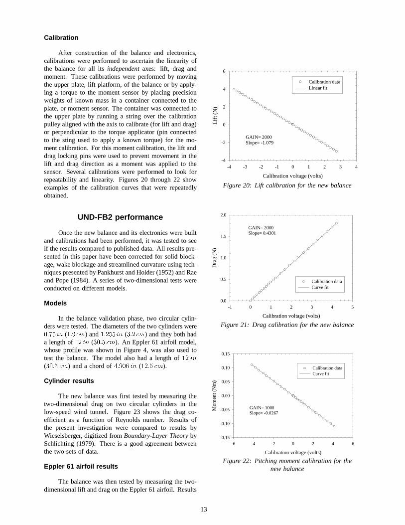
Calibration

After construction of the balance and electronics,calibrations were performed to ascertain the linearity ofthe balance for all itsindependentaxes: lift, drag andmoment. These calibrations were performed by movingthe upper plate, lift platform, of the balance or by apply-ing a torque to the moment sensor by placing precisionweights of known mass in a container connected to theplate, or moment sensor. The container was connected tothe upper plate by running a string over the calibrationpulley aligned with the axis to calibrate (for lift and drag)or perpendicular to the torque applicator (pin connectedto the sting used to apply a known torque) for the mo-ment calibration. For this moment calibration, the lift anddrag locking pins were used to prevent movement in thelift and drag direction as a moment was applied to thesensor. Several calibrations were performed to look forrepeatability and linearity. Figures 20 through 22 showexamples of the calibration curves that were repeatedlyobtained.

UND-FB2 performance

Once the new balance and its electronics were builtand calibrations had been performed, it was tested to seeif the results compared to published data. All results pre-sented in this paper have been corrected for solid block-age, wake blockage and streamlined curvature using tech-niques presented by Pankhurst and Holder (1952) and Raeand Pope (1984). A series of two-dimensional tests wereconducted on different models.

Models

In the balance validation phase, two circular cylin-ders were tested. The diameters of the two cylinders were LQ ( FP) and LQ ( FP) and they both hada length of LQ ( FP). An Eppler 61 airfoil model,whose profile was shown in Figure 4, was also used totest the balance. The model also had a length of LQ

( FP) and a chord of LQ ( FP).

Cylinder results

The new balance was first tested by measuring thetwo-dimensional drag on two circular cylinders in thelow-speed wind tunnel. Figure 23 shows the drag co-efficient as a function of Reynolds number. Results ofthe present investigation were compared to results byWieselsberger, digitized fromBoundary-Layer TheorybySchlichting (1979). There is a good agreement betweenthe two sets of data.

Eppler 61 airfoil results

The balance was then tested by measuring the two-dimensional lift and drag on the Eppler 61 airfoil. Results

Calibration voltage (volts)

-4 -3 -2 -1 0 1 2 3 4

Lift

(N

)

-4

-2

0

2

4

6

Calibration dataLinear fit

GAIN= 2000Slope= -1.079

Figure 20: Lift calibration for the new balance


-1 0 1 2 3 4 5

Dra

g (

N)

0.0

0.5

1.0

1.5

2.0

Calibration dataCurve fit

GAIN= 2000Slope= 0.4301

Figure 21: Drag calibration for the new balance


-6 -4 -2 0 2 4 6

Mom

ent (

Nm

)

-0.15

-0.10

-0.05

0.00

0.05

0.10

0.15

Calibration dataCurve fit

GAIN= 1000Slope= -0.0267

Figure 22: Pitching moment calibration for thenew balance

13

Re

1e+3 1e+4 1e+5

Cd

0.1

1

10

Small cylinderLarge cylinderWieselsberger (Schlichting, 1979)

Figure 23: 2D drag coefficient of two circular cylinderswith UND-FB2

were obtained in the wind tunnel and the water tunnel forseveral Reynolds numbers. Figures 24 and 25 show thetwo-dimensional lift and drag coefficients respectively inthe wind tunnel for differentnominalReynolds numbers,i.e., values used to adjust the velocity in the tunnel withthe model atm p.

Results for&O indicate a significant difference be-tween results at5HF ! and those for5HF

. For large5HF, &O increases smoothly with angleof attackm. For smaller5HF, the lift-curve slope&Om

is smaller forp m p and there is a sharp risein &O at m p. Similar results have been obtained byAlthaus (1980) and shown in Figure 26. Althaus useda strain gauge balance arrangement to measure lift and awake rake to measure drag. A drawback of using a wakerake will be addressed later. Althaus did observe a smallhysteresis loop at low Reynolds numbers. No apparenthysteresis was observed in the current study.

The sharp rise in&O at low Reynolds numbers isbelieved to be the result of a laminar separation bub-ble on the upper surface of the wing. O’Meara andMueller (1987) showed that the length of the separationbubble tends to increase with a reduction in5HF. A re-duction in the turbulence intensity also tends to increasethe length of the bubble. The lift-curve slope is affectedby separation bubbles. A longer bubble is usually associ-ated with a decrease in the lift-curve slope (Bastedo andMueller, 1985). This is the kind of behavior observedwith the Eppler 61 airfoil in this investigation. Flowvisualization by Mueller and Burns (1982) showed thepresence of a separation bubble on the Eppler 61 airfoilat 5HF .

In the water tunnel, the turbulence intensity is largerthan in the wind tunnel. Therefore, the smaller&Om andsharp rise in&O observed in the wind tunnel forp m p might not be present at all in the water tunneldata for the same Reynolds numbers. This is exactly

α (degrees)

-20 -10 0 10 20 30

Cl

-1.0

-0.5

0.0

0.5

1.0

1.5

2.0

Re= 42,000Re= 46,000Re= 62,300Re= 87,000

Figure 24: 2D lift coefficient on the Eppler 61 airfoil inthe wind tunnel with UND-FB2

α (degrees)

-20 -10 0 10 20 30

Cd

0.0

0.1

0.2

0.3

0.4

0.5

0.6

0.7

Re= 42,000Re= 46,000Re= 62,300Re= 87,000

Figure 25: 2D drag coefficient on the Eppler 61 airfoilin the wind tunnel with UND-FB2

what happened for5HF and5HF , asshown in Figure 27. The drag coefficient appears to beless affected, within the uncertainty of the measurements.Figure 28 shows the&G curves obtained in the watertunnel for the Eppler 61 airfoil.

Figures 29 through 31 show comparisons of the cur-rent Eppler 61 results with published data. There is, ingeneral, a good agreement between the current data andpublished data. The most significant difference is in thestall angle; there appears to be ap difference inmVWDOO.

Measurement uncertainty with UND-FB2

Uncertainties in the measurements were computedusing the Kline-McClintock technique (Kline and Mc-Clintock, 1953) for error propagation. As indicated ear-lier, the two main sources of uncertainty were the quanti-zation error and the uncertainty arising from the standarddeviation of a given mean output voltage. The quantiza-

14

Figure 26: Althaus’ results for 2D lift coefficient onthe Eppler 61 airfoil (Althaus, 1980)

tion error, described earlier, was smaller with the NIDAQcard than with the UEI card due to the better resolutionof the A/D converter (16 bits compared to 12 bits). Theuncertainty in the angle of attack was determined to be onthe order ofpb p. The error from the encoder wasnegligible. The encoder offered an excellent resolutionof 2,000 counts per degree, which gave an uncertainty ofdb. Figures 32 and 33 show a comparison of windtunnel and water tunnel results for the Eppler 61 airfoilat 5HF . Error bars indicate the uncertainty in&O and&G when the NIDAQ card is used. The averageuncertainties for&O and&G in the range of angles of at-tack tested are approximately in the water tunnel and in the wind tunnel.

The new balance in itself is also more sensitive thanthe old balance. This allows experiments at smaller ve-locities in the water tunnel. As of now, results with dif-ferent wings have shown a high degree of repeatability forReynolds numbers as low as . A major challengein measurements at Reynolds numbers below isbeing able to measure drag accurately. At5HF ,the minimum drag can be as low as1 , which corre-sponds to a load of approximately 2 grams. A fine dragcalibration of the balance showed that 1 gram was suf-ficient to deflect the drag flexure and yield a reasonableoutput voltage. However, this deflection is often on theorder of signal noise.

α (degrees)

-20 -10 0 10 20 30

Cl

-1.0

-0.5

0.0

0.5

1.0

1.5

2.0

Re= 42,000Re= 46,000

Figure 27: 2D lift coefficient on the Eppler 61 airfoil inthe water tunnel with UND-FB2

α (degrees)

-20 -10 0 10 20 30

Cd

0.0

0.1

0.2

0.3

0.4

0.5

0.6

0.7

Re= 42,000Re= 46,000

Figure 28: 2D drag coefficient on the Eppler 61 airfoilin the water tunnel with UND-FB2

Results for thin wings

This section will present results for thin flat andcambered wings. Some additional issues associated withdetermining aerodynamic characteristics as a function ofReynolds numbers will also be addressed. Accurate mea-surements of&O and&G with endplates and small aspect-ratio models are difficult to obtain at low Reynolds num-bers because of the interaction between the thick bound-ary layers on the endplates and the flow around the wing,which results into a three-dimensional flow along the spanof the model. This must be kept in mind when examiningthe following results.

Flat-plate wings

Some results for the flat-plate models (two endplatesfor 2D tests and one endplate for semi aspect-ratio tests)

15

α (degrees)

-20 -10 0 10 20 30

Cl

-1.0

-0.5

0.0

0.5

1.0

1.5

2.0

Re= 46,000 (wind tunnel)Re= 46,000 (Burns, 1981)Re= 40,000 (Althaus, 1980)

Figure 29: Comparison of 2D lift coefficient on theEppler 61 airfoil and published data with UND-FB2

Re= 46,000

α (degrees)

-20 -10 0 10 20 30

Cd

0.0

0.1

0.2

0.3

0.4

0.5

0.6

0.7

Current investigationBurns (1981)

Figure 30: Comparison of 2D drag coefficient on theEppler 61 airfoil and published data with UND-FB2

Cd

0.0 0.1 0.2 0.3 0.4 0.5 0.6 0.7

Cl

-1.0

-0.5

0.0

0.5

1.0

1.5

2.0

Re= 46,000Re= 40,000 (Althaus, 1980)

Figure 31: Comparison of 2D drag polar for the Eppler61 airfoil and published data with UND-FB2

Re= 42,000

α (degrees)

-20 -10 0 10 20 30

Cl

-1.0

-0.5

0.0

0.5

1.0

1.5

2.0

Wind tunnelWater tunnel

Figure 32: Comparison of the 2D lift coefficient on theEppler 61 airfoil in wind and water tunnels with UND-FB2

Re= 42,000

α (degrees)

-20 -10 0 10 20 30

Cd

0.0

0.1

0.2

0.3

0.4

0.5

0.6

0.7

Wind tunnelWater tunnel

Figure 33: Comparison of the 2D drag coefficient on theEppler 61 airfoil in wind and water tunnels with UND-FB2

can be seen in Figures 34 through 39 for5HF

and5HF . Figures 34 and 37 show a signifi-cant reduction in the lift-curve slope&/m for semi-infinitewings.

The lift-curve slope values obtained from the windtunnel data are compared to theoretical values for thinwings of different semi-span aspect ratios in Figure 40.Equation 1 from Anderson (1991) was used to estimatethe theoretical values of&/m :

&/m D D

bDe$5

c ~

(1)

whereD is the 2D lift-curve slope in 1/degrees,$5 isthe aspect ratio of the full wing ($5 e V$5) and ~is the Glauert parameter (equivalent to an induced dragfactor) varying typically between 0.05 and 0.25. The 2DvalueD was determined to beD GHJ. Thiscorresponds to the average of all the slopes&/m (for all

16

α (degrees)

-20 -10 0 10 20 30

Cl,

CL

-1.5

-1.0

-0.5

0.0

0.5

1.0

1.5

2DsAR= 3sAR= 1

Figure 34: Lift coefficient on flat plates at5HF with UND-FB1

α (degrees)

-20 -10 0 10 20 30

Cd,

CD

0.0

0.1

0.2

0.3

0.4

0.5

0.6

0.7

2DsAR= 3sAR= 1.5

Figure 35: Drag coefficient on flat plates at5HF with UND-FB1

α (degrees)

-20 -10 0 10 20 30

Cm

/4

-0.25

-0.20

-0.15

-0.10

-0.05

0.00

0.05

0.10

0.15

0.20

0.25

2DsAR= 3sAR= 1.5

Figure 36: Pitching moment coefficient on flat platesat 5HF with UND-FB1

α (degrees)

-20 -10 0 10 20 30

Cl,

CL

-1.5

-1.0

-0.5

0.0

0.5

1.0

1.5

2DsAR= 3sAR= 1.5sAR= 1sAR= 0.5

Figure 37: Lift coefficient on flat plates at5HF with UND-FB1

α (degrees)

-20 -10 0 10 20 30

Cd,

CD

0.0

0.1

0.2

0.3

0.4

0.5

0.6

0.7


Figure 38: Drag coefficient on flat plates at5HF with UND-FB1

α (degrees)

-20 -10 0 10 20 30

Cm

/4

-0.25

-0.20

-0.15

-0.10

-0.05

0.00

0.05

0.10

0.15

0.20

0.25


Figure 39: Pitching moment coefficient on flat plates at5HF with UND-FB1

17

1/sAR

0.00 0.25 0.50 0.75 1.00

CL

1/d

eg)

0.04

0.06

0.08

0.10

0.12

0.14

0.16

×

×

×

×

*

*

*

Re= 200,000Re= 180,000Re= 160,000Re= 140,000Re= 120,000Re= 100,000Re= 80,000×

Re= 60,000*

Theory: τ= 0.05

Theory: τ= 0.25

( )a

aa

a a

=+

+

=

0

0

0

157 3

1

2

* .

*

πτ

AR

AR sAR

and in degrees

Figure 40: Lift-curve slope for flat-plate models in windtunnel with UND-FB1

Reynolds numbers considered) for an infinite aspect ra-tio ( V$5 ). This value was picked instead of theconventional value ofD UDG GHJ given bythin-airfoil theory. Figure 40 shows a very good agree-ment between the experimental values of&/m and thetheoretical values estimated by Equation 1.

As the aspect ratio was decreased, Figures 34 and 37also show that the linear region of the&/ vs m curvebecame longer andmVWDOO tended to increase. Moreover,both figures show that there was no abrupt stall for lowaspect-ratio wings. For these low aspect ratios,&/ oftenreached a plateau and then remained relatively constant,or even started to increase, for increasing angles of attack.

Changing the aspect ratio of the models did notappear to have a measurable effect on the drag coef-ficient at 5HF , as shown in Figure 35. At5HF , increasing the aspect ratio had the unex-pected effect of increasing&' for angles greater thanp.No measurable difference was encountered in the rangebp m p.

Finally, Figures 36 and 39 show the pitching mo-ment at the quarter chord. Both figures indicate a slightlypositive slope&Pm

aroundm p, even when consider-ing the uncertainty. This would imply that the flat-platemodels were statically unstable aroundm p. Increas-ing the Reynolds number from to tendedto reduce the slope of&P . The model with a semi-span aspect ratio of 3 indicated an irregular behavior at5HF for &P ; the pitching moment was notzero atm p. This case will have to be repeated.

Aerodynamic characteristics as a function ofReynolds number: a different method

For tests without endplates, another balance arrange-ment, denoted arrangement number 3, was used and ispresented in Figure 41. The lift and drag forces measuredby the balance were for the wing-sting combination. Thelift on the sting was basically zero. However, the drag

of the sting alone, which dominated the total wing-stingdrag, was not zero and was subtracted from the wing-stingvalues to get the&' of the flat-plate wing alone.

U∞

Sting

Wing

24in(61cm)

8in(20.3cm)

Balance Straingauges

Lift platform

Drag platform

Base

Drag flexure

Figure 41: Balance arrangement (3) for finite wing testswith the new balance

In general, when investigators try to determine how&/PD[and&'PLQ

vary with Reynolds numbers, they deter-mine&/PD[

and&'PLQfrom &/ vsm and&' vsm curves

at different Reynolds numbers. It has been observed inthis investigation that the values obtained do not alwaysmatch the expected trend for drag because of the difficultyinvolved in measuring the very small drag forces. A slightoffset in one&/ vsm or&' vsm curve can lead to jagged&/PD[ vs 5HF or &'PLQ

vs 5HF curves. A better tech-nique was found to obtain&'PLQ

vs 5HF (the values of&/PD[ vs 5HF are of lesser importance because micro-airvehicles will rarely fly at&/PD[

). For this technique, theangle of attack was fixed to the angle yielding the lowest&' in a&' vsm curve, and measurements were taken fora series of increasing and decreasing Reynolds numberswithout stopping the tunnel. Results obtained with thenew balance UND-FB2 using this technique on a finitewing of aspect ratio$5 in the wind tunnel, pre-sented in Figures 42 and 43, are promising and the trendsobtained matched the expected reduction in&'PLQ

withincreasing Reynolds numbers.

18

Re

0 50000 100000 150000 200000 250000

CL

0.0

0.1

0.2

0.3

0.4

0.5

α= 0°α= 3°α= 10°

Figure 42: Lift coefficient variation with5H for$5 flat-plate wing with UND-FB2

Re

0 50000 100000 150000 200000 250000

CD

0.000

0.005

0.010

0.015

0.020

0.025

0.030

0.035

0.040

0.045

0.050

0.055

α= 0°

α= 3°Theory

CD = 1328 2. *

Re

(a) m p andp

Re

0 50000 100000 150000 200000 250000

CD

0.00

0.02

0.04

0.06

0.08

0.10

0.12

0.14

0.16

0.18

α= 10°

(b) m p

Figure 43: Drag coefficient variation with5H for$5 flat-plate wing with UND-FB2

Results at the angle of attack forb/'

cPD[

(m p) alsoshow an increase in&/ and a decrease in&' with in-creasing Reynolds number. The results of Figure 42 atm p are smaller than the lift coefficient presented inFigure 34 for a model withV$5 because of the lackof an endplate. For a given model, adding an endplateleads to an increase in lift compared to the case withoutan endplate, as shown in Figure 44. Adding one end-plate did not have a significant effect on&', as shownin Figure 45. The wing used for this series of tests had anominal chordF LQ and spanE LQ [C8S12].

Re

0 50000 100000 150000 200000 250000

CL

0.11

0.12

0.13

0.14

0.15

0.16

0.17

0.18

0.19

1 endplateNo endplate

Figure 44: Lift coefficient variation with Re (C8S12)with UND-FB2 atm p

Re

0 50000 100000 150000 200000 250000

CD

0.00

0.01

0.02

0.03

0.04

0.05

0.06

0.07

1 endplateNo endplate


At an angle of attackm p, adding one or twoendplates did not affect&/ for 5HF ! ; it re-mained basically around the expected value of zero, asshown in Figure 46. Moreover, adding endplates did not,once again, have a measurable effect on&', as presentedin Figure 47. Since Figure 47 is form p, it represents&'PLQ

versus Reynolds number for flat-plate wings. Ex-perimental results are also compared to theory (Blasius:&'PLQ

e S5H) and CFD results in Figure 47.

19

The CFD results were computed by Greg Brooks (AirForce Research Laboratory, Wright-Patterson Air ForceBase) using COBALT, a parallel, implicit, unstructured,finite volume CFD code based on Godunov’s exact Rie-mann method, developed by theAir Force Research Lab-oratory (see Strang, Tomaro and Grismer, 1999). All setsof data indicate the same trend. The experimental datawas always larger than theory and the CFD results. Thiscould have been caused by surface roughness, imperfectflow conditions, and so forth. Since all wind tunnel testswith the flat and cambered wings are usually conductedat Reynolds numbers greater than , the results pre-sented in Figures 42 through 47 for5H shouldbe analyzed with caution. The velocity in the wind tun-nel is usually too low for5H to yield reliableresults.

Re

0 50000 100000 150000 200000 250000

Cl,

CL

-0.10

-0.05

0.00

0.05

0.10

0.15

0.20

2 endplates1 endplateNo endplate


Re

0 50000 100000 150000 200000 250000

Cd,

CD

0.000

0.005

0.010

0.015

0.020

0.025

0.030

0.035

0.040

0.045

0.050

0.055

2 endplates1 endplateNo endplateBlasius solutionCOBALT (Brooks, 1999)

Figure 47: Drag coefficient variation with Re (C8S12)with UND-FB2 atm p

The results of Figure 47 seem to indicate that forthin flat-plate wings atm p the drag coefficient actingon the wing is independent of aspect ratio. Results ofFigure 47 were then compared to the drag coefficients

Re

0 50000 100000 150000 200000 250000

Cd,

CD

0.000

0.005

0.010

0.015

0.020

0.025

0.030

0.035

0.040

0.045

0.050

0.055

2DsAR= 1.5AR= 1.5AR= 1Blasius solutionCOBALT (Brooks, 1999)

Figure 48: Minimum drag coefficient with5H for$5 w flat-plate wings with UND-FB2

for the $5 plate and no difference was obtained,as shown in Figure 48. For aspect ratios greater thanone, the minimum drag coefficient is then independentof model size and the presence of endplates. For loweraspect ratios, preliminary tests indicated a larger&'PLQ

.More work is in progress to fully understand the behaviorof &'PLQ

as a function of Reynolds numbers for the verylow aspect-ratio wings ($5 ). Similar tests will alsohave to be conducted on the cambered wings. The non-measurable difference in&'PLQ

with Reynolds numbersmight just be valid for flat-plate wings. Adding cambermight change the results. Preliminary results seem toindicate this trend.

Cambered-plate wings

Results were also obtained for cambered-plate mod-els using the balance arrangement with one or two end-plates (semi-infinite or 2D tests). In general, camberled to better aerodynamic characteristics due to an in-crease in lift, even though drag also increased. Figures 49through 54 show some results for the cambered plates at5HF and 5HF . With camberedplates,&'PLQ

was slightly larger than for flat plates. Themaximum lift coefficient was also larger, as expected.Moreover, the variation in&/ with angle of attack atsmall angles was less linear for cambered plates than forflat plates. Finally, the behavior of the moment coefficient&P for the cambered plates was very different than thebehavior with the flat plates. A rise in&P occurredafterm p, leading to a hump at aroundm p. Thiswas not observed with the flat plates. Flow visualizationwill hopefully explain this behavior.

Equation 1 was also used to compare the experi-mental values of&/m at m&/ for the cambered platesto theoretical values. The 2D valueD used wasD GHJ. Figure 55 shows a good agreement betweentheory and experiments.

20

α (degrees)

-20 -10 0 10 20 30

Cl,

CL

-1.5

-1.0

-0.5

0.0

0.5

1.0

1.5

2DsAR= 3sAR= 1.5

Figure 49: Lift coefficient on cambered plates at5HF with UND-FB1

α (degrees)

-20 -10 0 10 20 30

Cd,

CD

0.0

0.1

0.2

0.3

0.4

0.5

0.6

0.7

2DsAR= 3sAR= 1.5

Figure 50: Drag coefficient on cambered plates at5HF with UND-FB1

α (degrees)

-20 -10 0 10 20 30

Cm

/4

-0.25

-0.20

-0.15

-0.10

-0.05

0.00

0.05

0.10

0.15

0.20

0.25

2DsAR= 3sAR= 1.5

Figure 51: Pitching moment coefficient on camberedplates at5HF with UND-FB1

α (degrees)

-20 -10 0 10 20 30

Cl,

CL

-1.5

-1.0

-0.5

0.0

0.5

1.0

1.5

2DsAR= 3sAR= 1.5sAR= 1

Figure 52: Lift coefficient on cambered plates at5HF with UND-FB1

α (degrees)

-20 -10 0 10 20 30

Cd,

CD

0.0

0.1

0.2

0.3

0.4

0.5

0.6

0.7


Figure 53: Drag coefficient on cambered plates at5HF with UND-FB1

α (degrees)

-20 -10 0 10 20 30

Cm

/4

-0.25

-0.20

-0.15

-0.10

-0.05

0.00

0.05

0.10

0.15

0.20

0.25


Figure 54: Pitching moment coefficient on camberedplates at5HF with UND-FB1

21

1/sAR

0.00 0.25 0.50 0.75 1.00

CL

(1/d

eg)

0.04

0.06

0.08

0.10

0.12

0.14

0.16

×

×

*

*

*

Re= 200,000Re= 180,000Re= 160,000Re= 140,000Re= 120,000Re= 100,000Re= 80,000×

Re= 60,000*

Theory: τ= 0.05

Theory: τ= 0.25

( )a

aa

a a

=+

+

=

0

0

0

157 3

1

2

* .

*

πτ

AR

AR sAR

and in degrees

Figure 55: Lift-curve slope for cambered-plate modelsin wind tunnel with UND-FB1

Since the cambered wings showed better aerody-namic characteristics, and hence are more suitable in thedesign of micro-air vehicles, only performance data forthe cambered plates is presented. Figures 56 through 59show the behavior of&/PD[

, &'PLQ,

b/'

cPD[

andt&

/

&'

uPD[

as a function of Reynolds number. The max-

imum / ' ratio is related to the maximum range for a

propeller driven airplane, while the maximum& / &'

is related to best endurance (longest flying time possi-ble). As expected,&/PD[

increased with Reynolds numberand aspect ratio in the range of Reynolds numbers tested.The same expected behavior was obtained for

b/'

cPD[

andt&

/

&'

uPD[

. On the other hand,&'PLQshowed an in-

crease with decreasing Reynolds number, as was also ex-pected. The maximum/ ' generally occurred atm p

to p, while

t&

/

&'

uPD[

occurred atm p to p. It

is important to remember that the endplates have beenshown to have an effect on the lift coefficients of flat-plate wings, and probably cambered-plate wings also. Asmentioned earlier, the effect of the endplates on the dragcharacteristics of cambered-plate wings is still under in-vestigation. The results presented in this report must thenbe analyzed with the possible effect of the endplates inmind; the numerical values should not be taken as the ul-timate results. The effect of the endplates on the pitchingmoment has not been investigated for both flat-plate andcambered-plate wings.

Effect of trailing-edge geometry

Four models [F LQ (F FP) andE LQ(E FP)] were tested in the wind tunnel at sev-eral chord Reynolds numbers to see if the trailing-edgegeometry had any influence on the aerodynamic charac-teristics of flat plates and cambered plates at low chord

Rec

0 50000 100000 150000 200000

Cl m

ax, C

Lm

ax

0.00

0.25

0.50

0.75

1.00

1.25

1.50

2DsAR= 1.5sAR= 1

Figure 56: Maximum lift coefficient as a function of5HF for cambered wings with UND-FB1

Rec

0 50000 100000 150000 200000

Cd m

in, C

Dm

in

0.00

0.01

0.02

0.03

0.04

0.05

2DsAR= 1.5

Figure 57: Minimum drag coefficient as a functionof 5HF for cambered wings with UND-FB1

Rec

0 50000 100000 150000 200000

( L/D

) ma

x

0

5

10

15

20

25

30


Figure 58: Maximum/ ' ratio as a function of5HF

for cambered wings with UND-FB1

22

Rec

0 50000 100000 150000 200000

(CL

3/2 /C

D) m

ax

0

5

10

15

20

25

30


Figure 59: Maximum& / &' ratio as a functionof 5HF for cambered wings with UND-FB1

Reynolds numbers. The first two models had a taperedtrailing edge, while the other two models had an ellipti-cal trailing edge. Results were obtained for infinite mod-els (2D case) and models with a semi-span aspect ratioV$5 . For both cases, no significant difference wasobserved in&/ or &O, and&' or &G, as a function oftrailing-edge geometry, as shown in Figures 60 and 61 for5HF . A difference was however observed inthe moment coefficient&P . For a sharp trailing edge,&Pm

often appeared to be positive aroundm p, evenwith the uncertainty considered (error bars in&P areabout the size of the symbols). With the elliptical trailingedge, the 2D cases at5HF showed a stablenegative value of&Pm

, as shown in Figure 62. For asemi-span aspect ratio of 1.5,&Pm

was basically zero atm p. Flow visualization to be performed later mayexplain this phenomenon.

With the cambered plates, there was basically nodifference between a sharp trailing edge and an ellipticaltrailing edge at5HF , as shown in Figures 63through 65. Results with the cambered plates seem toagree with Laitone (Laitone, 1996 and 1997), who showedthat at low Reynolds numbers, a sharp trailing edge is notas critical as for larger Reynolds numbers.

The influence of the leading-edge geometry was alsoinvestigated by looking at the lift and drag characteristicsof a flat-plate model in 2D andV$5 configurationsin the water tunnel at5HF and5HF .For these tests, the existing C8S12 model was rotated 180degrees (tapered leading edge and elliptical trailing edge).No difference was noticed in the results for lift and drag.Laitone (1996 and 1997) did notice a significant increasein lift at 5HF for a thicker reversed NACA0012 airfoil (the sharp trailing edge was facing the flow).Further tests will be conducted in the wind tunnel at largerReynolds numbers on flat-plate and cambered-plate wingsto complete this study of the leading-edge geometry effect

α (degrees)

-20 -10 0 10 20 30

Cl,

CL

-1.5

-1.0

-0.5

0.0

0.5

1.0

1.5

2D: sharp TE2D: elliptical TEsAR= 1.5: sharp TEsAR= 1.5: elliptical TE

Figure 60: Trailing-edge geometry effect on liftcoefficient at5HF on flat plates in the

wind tunnel with UND-FB1

α (degrees)

-20 -10 0 10 20 30

Cd,

CD

0.0

0.1

0.2

0.3

0.4

0.5

0.6

0.7


Figure 61: Trailing-edge geometry effect on dragcoefficient at5HF on flat plates in the


α (degrees)

-20 -10 0 10 20 30

Cm

/ 4

-0.25

-0.20

-0.15

-0.10

-0.05

0.00

0.05

0.10

0.15

0.20

0.25


Figure 62: Trailing-edge geometry effect on pitchingmoment coefficient at5HF on flat plates

in the wind tunnel with UND-FB1

23

α (degrees)

-20 -10 0 10 20 30

Cl,

CL

-1.5

-1.0

-0.5

0.0

0.5

1.0

1.5


Figure 63: Trailing-edge geometry effect on liftcoefficient at5HF on cambered plates in the


α (degrees)

-20 -10 0 10 20 30

Cd,

CD

0.0

0.1

0.2

0.3

0.4

0.5

0.6

0.7


Figure 64: Trailing-edge geometry effect on dragcoefficient at5HF on cambered plates in the


α (degrees)

-20 -10 0 10 20 30

Cm

/4

-0.25

-0.20

-0.15

-0.10

-0.05

0.00

0.05

0.10

0.15

0.20

0.25


Figure 65: Trailing-edge geometry effect on pitchingmoment coefficient at5HF on cambered plates

in the wind tunnel with UND-FB1

on the aerodynamic characteristics of thin wings/airfoils.

Effect of freestream turbulence

Mueller et al. (1983) showed that an increase infreestream turbulence intensity reduced the minimum dragacting on an thick Lissaman 7769 airfoil at5HF

and slightly increased&OPD[ . This was causedby an earlier laminar shear layer transition, hence earlierflow reattachment (i.e., a shorter separation bubble), witha larger turbulence intensity. At large angles of attackwhere the flow is mostly separated, they observed an in-crease in drag coefficient with an increase in turbulenceintensity. Increasing the turbulence intensity also helpedto eliminate some of the hysteresis encountered in&O and&G for that particular airfoil.

Pohlen (1983) also looked at the influence of turbu-lence intensity on a thick Miley airfoil (M06-13-128)(see Miley, 1972). He found that increasing the turbu-lence intensity helped to reduce the hysteresis in&O and&G and slightly improved airfoil performance.

Tests were then conducted in the wind tunnel withdifferent screens upstream of the flat-plateV$5

models and a flow restrictor downstream of the model tosee if a difference in the turbulence intensity could resultin different aerodynamic properties for the models usedin this investigation. The flow restrictor, or strawbox,was made of drinking straws packed in a wooden frameand placed between the test section and the diffuser. Theadditional turbulence intensity generated by the strawboxwas determined to be approximately (Brendel andHuber, 1984). Table 3 indicates the mesh size and nomi-nal freestream turbulence intensity in the test section withonly a screen present (no flow restrictor).

Screen Mesh size Wire Turbulence(PHVKHV FP) diameter %

(PP)

Fine 7.09 0.245 0.25Medium 3.15 0.508 0.45Coarse 0.64 1.397 1.3

Table 3: Turbulence screen data(Pohlen, 1983; and Brendel and Huber, 1984)

No measurable differences were observed in the re-sults for different turbulence intensities at5HF

on the V$5 flat-plate model, as shown in Fig-ures 66 and 67. Only a slight increase in&/PD[

and anincrease in&' for large angles of attack was noticedfor the case with the fine mesh and with the strawbox.All other cases gave the same results. Therefore, the ef-fect of turbulence intensity appeared to be minimal in thewind tunnel for the models tested. Similar results were

24

α (degrees)

-20 -10 0 10 20 30

CL

-1.5

-1.0

-0.5

0.0

0.5

1.0

1.5

No screen, no strawboxNo screen, with strawboxFine mesh, with strawboxMedium mesh, with strawboxCoarse mesh, with strawbox

Figure 66: Freestream turbulence effect on lift coefficientat 5HF in the wind tunnel for theV$5

flat-plate model with UND-FB1

α (degrees)

-20 -10 0 10 20 30

CD

0.0

0.1

0.2

0.3

0.4

0.5

0.6

0.7

No screen, no strawboxNo screen, with strawboxFine mesh, with strawboxMedium mesh, with strawboxCoarse mesh, with strawbox

Figure 67: Freestream turbulence effect on dragcoefficient at5HF in the wind tunnel for the

V$5 flat-plate model with UND-FB1

obtained at5HF in the wind tunnel, and at5HF and5HF in the water tunnel.

Effect of endplates on 2D measurements

It has been shown in previous experiments at NotreDame that the presence of the endplates during 2D testsusually leads to a larger&'PLQ

. For an 18% thick airfoil(NACA b ), Mueller and Jansen (1982) showedthat the interaction between the endplates and the modelresulted in a 20% increase in&GPLQ

at Reynolds numbersbetween and .

Since most of the tests in the current investiga-tion were conducted at very low speeds, the interactionbetween the boundary layer growing on the endplatesand the wing created acorner flow, as depicted in Fig-ure 68, which acted over a significant portion of the wingspan and significantly altered the 2-dimensionality of the

U∞

Figure 68: Schematic of corner flow on wing

flow over the wing. This phenomenon of the cornerflow has been investigated by several authors, includingHawthorne (1954) and Barber (1978) who looked at theflow around struts near a wall.

In order to verify the effect of the endplates on theaerodynamic characteristics of the Eppler 61 airfoil, a3-piece Eppler 61 model was used. With this setup, asection of an Eppler 61 model was free to move betweentwo other sections of the same airfoil. These two othersections were fixed to the endplates in the wind tunnel,as shown in Figure 69, at the same angle of attack asthe middle section. A small gap was present between theend models and the center piece connected to the forcebalance. Figure 70 shows the three pieces of the 3-pieceEppler 61 model.

The angle of attack of the 3-piece Eppler 61 modelwas adjusted to a certain value and the velocity in thetunnel, hence the Reynolds number, was varied. The be-havior of &G and&O was measured. From the previous2D results on the Eppler 61 airfoil, it was determinedthat&GPLQ occurred atm p and the angle for zero liftwas aboutm bp. The behavior of&G vs 5HF wasfirst obtained at these two angles of attack. Figures 71and 72 show that the drag coefficient with the 3-pieceEppler 61 model was much smaller than with the fullmodel. This result is similar to that reported by Muellerand Jansen (1982) for the NACA b airfoil. Thelift coefficient with the 3-piece model was higher thanwith the full model. The aerodynamic characteristics withthe 3-piece model were closer to true 2-dimensional re-sults, where a larger&O and smaller&G would normallybe expected. The behavior of&O and&G with Reynoldsnumbers also followed the expected trends. A reductionin &G and an increase in&O were observed with increas-ing Reynolds numbers. Results from Althaus (1980) andde Vries et al. (1980) are also included in the figuresfor comparison. As was mentioned earlier for Althaus,

25

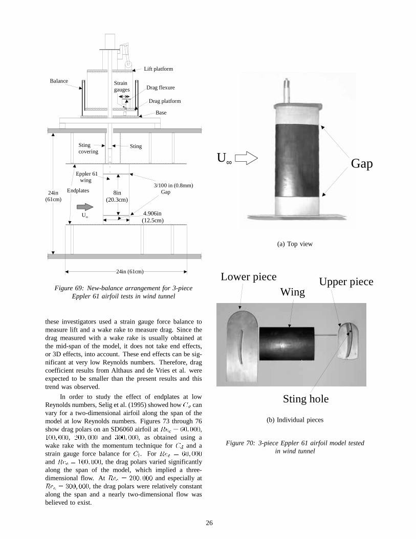
Endplates

U∞

StingStingcovering

Eppler 61 wing

3/100 in (0.8mm) Gap

24in (61cm)

24in(61cm)

4.906in(12.5cm)

Balance Straingauges

Lift platform

Drag platform

Base

Drag flexure

8in (20.3cm)

Figure 69: New-balance arrangement for 3-pieceEppler 61 airfoil tests in wind tunnel

these investigators used a strain gauge force balance tomeasure lift and a wake rake to measure drag. Since thedrag measured with a wake rake is usually obtained atthe mid-span of the model, it does not take end effects,or 3D effects, into account. These end effects can be sig-nificant at very low Reynolds numbers. Therefore, dragcoefficient results from Althaus and de Vries et al. wereexpected to be smaller than the present results and thistrend was observed.

In order to study the effect of endplates at lowReynolds numbers, Selig et al. (1995) showed how&G canvary for a two-dimensional airfoil along the span of themodel at low Reynolds numbers. Figures 73 through 76show drag polars on an SD6060 airfoil at5HF , , and , as obtained using awake rake with the momentum technique for&G and astrain gauge force balance for&O. For 5HF

and5HF , the drag polars varied significantlyalong the span of the model, which implied a three-dimensional flow. At5HF and especially at5HF , the drag polars were relatively constantalong the span and a nearly two-dimensional flow wasbelieved to exist.

GapU∞

(a) Top view

Lower piece Upper piece

Sting hole

Wing

(b) Individual pieces

Figure 70: 3-piece Eppler 61 airfoil model testedin wind tunnel

26

Re

20000 40000 60000 80000 100000 120000

Cl

0.30

0.35

0.40

0.45

0.50

0.55

0.60

0.65

0.703-piece airfoil1-piece airfoilAlthaus (1980)de Vries et al. (1980)

(a) Lift coefficient

Re

20000 40000 60000 80000 100000 120000

Cd

0.00

0.01

0.02

0.03

0.04

0.05

0.06

0.07

0.08

3-piece airfoil1-piece airfoilAlthaus (1980)de Vries et al. (1980)

(b) Drag coefficient

Figure 71: Endplates effect on 2D characteristics ofEppler 61 airfoil atm p with UND-FB2

Re

20000 40000 60000 80000 100000 120000C

l-0.05

0.00

0.05

0.10

0.15

0.20

0.25

3-piece airfoil1-piece airfoilAlthaus (1980)


Re

20000 40000 60000 80000 100000 120000

Cd

0.02

0.03

0.04

0.05

0.06

0.07

0.08

0.09



Figure 72: Endplates effect on 2D characteristics ofEppler 61 airfoil atm bp with UND-FB2

27

Figure 73: Drag polar for SD6060 airfoil at5HF (Selig et al., 1995)




28

(a) Oil flow on Clark Y airfoil at5HF d (Peake and Tobak, 1982)

(b) Conjectures pattern of skin-friction lines(Peake and Tobak, 1982)

Figure 77: Flow pattern over a rectangular wing ofaspect ratio 3.5 at angle of attack beyond stall

For semi-infinite models, and also for finite models,the flow is highly three-dimensional, as was shown byWilliams (1996) for low aspect-ratio wings at high anglesof attack and Winkelman and Barlow (1980), whose workwas reviewed by Peake and Tobak (1982). Figure 77shows the flow pattern over a finite rectangular wing atan angle of attack beyond stall.

Other results for the 3-piece Eppler 61 model indi-cated that the zero-lift angle of attack was close tobpinstead ofm bp, so tests were conducted at the newzero-lift angle of attack, as shown in Figure 78.

For the full model, it was determined that/ 'PD[occurred atm p. The 3-piece model was then testedat an angle of attack ofp. Unfortunately, the lift forceacting on the middle section of the model became largeenough at larger Reynolds numbers to deflect the lower tipof the section, which resulted in a poor alignment with thefixed bottom part of the model. Some three-dimensionaleffects were then believed to be created, which yielded re-sults that did not follow a two-dimensional trend: the liftcoefficient started to decrease with increasing Reynolds

Re

20000 40000 60000 80000 100000 120000

Cl

-0.14

-0.12

-0.10

-0.08

-0.06

-0.04

-0.02

0.00

0.02

0.04

0.06

0.08



Re

20000 40000 60000 80000 100000 120000

Cd

0.02

0.03

0.04

0.05

0.06

0.07

0.08

0.09

0.10



Figure 78: Endplates effect on 2D characteristics ofEppler 61 airfoil atm bp with UND-FB2

number. It is known that a semi-infinite model, wherethe bottom endplate has been removed, will have a lowerlift coefficient than an infinite model, or pseudo-infinitemodel. Figure 79 shows the results atm p. It is in-teresting to note the significant increase in&O just before5HF . This larger lift coefficient at Reynoldsnumbers greater than was mentioned earlier whenlooking at the behavior of&O with angle of attack for dif-ferent Reynolds numbers.

Conclusions

It has been shown that sensitive equipment mustbe used to perform aerodynamic measurements on smallmodels at very low Reynolds numbers. To achieve thisgoal, a new platform aerodynamic balance was designed

29

Re

20000 40000 60000 80000 100000 120000

Cl

0.8

0.9

1.0

1.1

1.2

1.3

1.4

1.5

3-piece airfoil1-piece airfoilAlthaus (1980)de Vries et al. (1980)


Re

20000 40000 60000 80000 100000 120000

Cd

0.00

0.02

0.04

0.06

0.08

0.10

0.12

0.14

0.16

0.183-piece airfoil1-piece airfoilAlthaus (1980)de Vries (1980)


Figure 79: Endplates effect on 2D characteristics ofEppler 61 airfoil atm p with UND-FB2

and built at the University of Notre Dame. The balanceshows good sensitivity, repeatability and accuracy. Tech-niques to reduce noise and increase the accuracy of theresults in the water tunnel below Reynolds numbers of are still being investigated.

Moreover, it has been shown that cambered-platewings with camber offer better aerodynamic charac-teristics than flat-plate wings for a given Reynolds num-ber. Reducing the Reynolds number can lead to poorperformance due to the large reduction in

b/'

cPD[

andt&

/

&'

uPD[

for both flat- and cambered-plate wings.

The turbulence intensity in the tunnel and thetrailing-edge geometry have been shown to have a verysmall effect on the measurements of lift, drag and pitch-ing moment on the thin models tested in this investigation.However, the presence of endplates can affect the resultsfor lift and drag due to the interaction between the bound-

ary layer growing on the endplate and the flow around thewing. The presence of endplates at low Reynolds num-bers reduces the 2D lift and increases the 2D drag thatwould normally be obtained with a truly infinite model,according to tests on the Eppler 61 airfoil. Furthermore,for a given model, adding one endplate leads to an in-crease in lift compared to the case without an endplate.Testing finite wing models without endplates appears tobe desirable at low Reynolds numbers because it elim-inates endplate effects. The full effect of the endplatesis still under investigation, especially for cambered-platewings.

Finally, trends of&'PLQversus5HF should be inves-

tigated by fixing the wing at the angle of attack yield-ing &'PLQ

and then varying the wind velocity, hence theReynolds number, in the tunnel. This seems to help toeliminate scatter in the results. Tests using this techniqueon various flat plates have indicated the expected trendsof a reduction in&'PLQ

and an increase in&/ with anincrease in Reynolds number.

Acknowledgements

This research was sponsored by the U.S. Navy,Naval Research Laboratory, Washington, D.C. under Con-tract No. N00173-98-C-2025 and the Roth-Gibson En-dowment at the University of Notre Dame. The authorwould like to thank Alain Pelletier for his effort and ex-pertise in the experimental phase of this study as well ashis help in preparing this manuscript. Special thanks goto Matthew Keennon ofAeroVironment, William Davis,Jr. of The Lincoln Laboratory, Jeffrey Harris ofSanders,A Lockheed Martin Company, and Kevin Ailinger of theNaval Research Laboratoryfor sharing the results of theirMAV development projects. Permission by Dr. M. Seligto used his wake rake data andThe Lincoln Laboratoryfor Figure 2 is gratefully acknowledged.

References

Ailinger, K. G. “U.S. Navy Micro Air Vehicle De-velopment.” Unmanned Air Vehicle Systems Four-teenth International Conference, April 1999: 36-1–36-7.

Althaus, Dieter. Profilpolaren fur den Modellflug.Neckar-Verlag, Institut fur Aerodynamik und Gas-dynamik, University of Stuttgart, 1980.

Anderson, John D., Jr. Fundamentals of Aerodynam-ics. QG ed. New York: McGraw-Hill, 1991.

Ashley, S.“Palm-Size Spy Planes.”Mechanical Engi-neering, February 1998: 74-78.

Barber, T. J. “An Investigation of Strut-Wall Intersec-tion Losses.”Journal of Aircraft,Vol. 15, No. 10,October 1978: 676-681.

30

Bastedo, W. G. Jr., and T. J. Mueller. “The Span-wise Variation of Laminar Separation Bubbles onFinite Wings at Low Reynolds Numbers.” AIAAPaper #85-1590, July 1985.

Batill, Stephen M., and Thomas J. Mueller.“Visual-ization of the Laminar-Turbulent Transition in theFlow Over an Airfoil Using the Smoke-Wire tech-nique.” AIAA Paper #80-0421, March 1980.

Brendel, Michael, and Arthur F. Huber II. “An Ex-perimental Investigation of Flow Quality in an In-draft Subsonic Wind Tunnel Using a Single HotWire Anemometer.” University of Notre Dame,November 1984.

Brooks, Gregory Air Force Research Laboratory, Pri-vate Communication, June 1999.

Burns, Thomas F. “Experimental Studies of Eppler61 and Pfenninger 048 Airfoils at Low ReynoldsNumbers.” Master’s Thesis, The University ofNotre Dame, January 1981.

Carmichael, B. H. “Low Reynolds Number Air-foil Survey.” Volume I, NASA Contractor Report165803, November 1981.

Davis, W. R., Jr., B. B. Kosicki, D. M. Boroson, andD. F. Kostishack. “Micro Air Vehicles for Opti-cal Surveillance.”The Lincoln Laboratory Journal,Vol. 9, No. 2, 1996: 197-213.

Davis, W. R., Jr. The Lincoln Laboratory, PrivateCommunication, June 1999.

de Vries, J., G. H. Hegen, and L. M. M. Boermans.“Preliminary Results of Windtunnel Measurementsat Low Reynolds Numbers on Airfoil Section E61.”Intern Report LSW 80-5, 1980.

Dornheim, M. A. “Unmanned Aerial Vehicles: TinyDrones May Be Soldiers’ New Tool.”AviationWeek & Space Technology, June 8, 1998: 42-48.

EideticsU. Operations Manual: Flow VisualizationWater Tunnel.

Fulghum, D. A. “Miniature Air Vehicles Fly IntoArmy’s Future.” Aviation Week & Space Technol-ogy, November 9, 1998: 37-38.

Harris, J. D. Sanders, A Lockheed Martin Company,Private Communication, 1999.

Hawthorne, W. R. “The Secondary Flow About Strutsand Airfoils.” Journal of the Aeronautical Sci-ences, Vol. 21, No. 1, January 1954: 588-608.

Huber, Arthur F., II. “The Effects of Roughness onan Airfoil at Low Reynolds Numbers.” Master’sThesis, The University of Notre Dame, May 1985.

Jackson, Paul, ed.Jane’s All the World’s Aircraft.Jane’s Information Group, 1996-97.

Keennon, M. AeroVironment, Private Communication,June 1999.

Kline, S. J., and F. A. McClintock. “DescribingUncertainties in Single-Sample Experiments.”Me-chanical Engineering, Vol. 75, No. 1, January1953: 3-8.

Laitone, E. V. “Aerodynamic Lift at Reynolds Num-bers Belowd.” AIAA Journal,Vol. 34, No. 9,September 1996: 1941-1942.

Laitone, E. V. “Wind Tunnel Tests of Wings atReynolds Numbers Below 70,000.”Experiments inFluids, Vol. 23, 1997: 405-409.

McMasters, J. H., and M. L. Henderson. “LowSpeed Single Element Airfoil Synthesis.”Tech.Soaring,Vol. 2, No. 2, 1980: 1-21.

Miley, S. J. “An Analysis of the Design of AirfoilSections for Low Reynolds Numbers.” Ph.D. Dis-sertation, Mississippi State University, 1972.

Morris, S. J. “Design and Flight Test Results forMicro-Signed Fixed-Wing and VTOL Aircraft.”VW International Conference on Emerging Tech-nologies for Micro Air Vehicles, Georgia Instituteof Technology, Atlanta Georgia, February 1997:117-131.

Mraz, S. J. “Honey I Shrunk the Plane.”Machine De-sign, October 1998: 35-42.

Mueller, T. J., and T. F. Burns. “Experimental Stud-ies of the Eppler 61 Airfoil at Low Reynolds Num-bers.” AIAA Paper #82-0345, January 1982.

Mueller, T. J., and B. J. Jansen, Jr. “AerodynamicMeasurements at Low Reynolds Numbers.” AIAAPaper #82-0598, March 1982.

Mueller, T. J., L. J Pohlen, P. E. Conigliaro, and B.J. Hansen, Jr.“The Influence of Free-Stream Dis-turbances on Low Reynolds Number Airfoil Ex-periments.”Experiments in Fluids.Vol. 1, 1983:3-14.

O’Meara, M. M., and T. J. Mueller. “Laminar Sepa-ration Bubble Characteristics on an Airfoil at LowReynolds Numbers.”AIAA Journal,Vol. 25, No. 8,August 1987: 1033-1041.

Pankhurst, R. C., and D. W. Holder. Wind-TunnelTechnique.London: Sir Isaac Pitman & Sons,1952.

31

Peake, David J., and Murray Tobak. “Three-Dimensional Flows About Simple Components atAngle of Attack.” AGARD Lecture Series No. 121on High Angle-of-Attack Aerodynamics, Paper No.2, 1982.

Pelletier, Alain. “A Study of the Nonlinear Aerody-namic Characteristics of a Slender Double-DeltaWing in Roll.” Ph.D. Dissertation, The Universityof Notre Dame, April 1998.

Pohlen, Lawrence.“Experimental Studies of the Ef-fect of Boundary Layer Transition on the Perfor-mance of the Miley (M06-13-128) Airfoil at LowReynolds Numbers.” Master’s Thesis, The Univer-sity of Notre Dame, January 1983.

Prazak, M. W., and T. J. Mueller. “ExperimentalStudies of an Eppler 61 Wing at Chord ReynoldsNumbers from 12,000 to 63,000.” Technical NoteUNDAS-TN-256-1, July 1997.

Rae, William H. Jr., and Alan Pope.Low-Speed WindTunnel Testing.QG ed. New York: John Wiley &Sons, 1984.

Schlichting, Hermann. Boundary-Layer Theory.WK

ed. New York: McGraw-Hill, 1979.

Selig, Michael S., et al.Summary of Low-Speed AirfoilData. Volume 1, Virginia: SoarTech Publications,1995.

Strang, W. Z., R. F. Tomaro, and M. J. Grismer.“The Defining Methods of Cobalt60: A Parallel,Implicit, Unstructured Euler/Navier-Stokes FlowSolver.” AIAA Paper #99-0786, January 1999.

Taylor, John W.R., ed.Jane’s All the World’s Aircraft.Jane’s Information Group, 1969-70.

Tennekes, Henk.The Simple Science of Flight: FromInsects to Jumbo Jets.Cambridge: The MIT Press,1996.

Williams, David L., III. “Dynamic, Lateral Behaviorof Low-Aspect-Ratio, Rectangular Wings at HighAngles of Attack.” Ph.D. Dissertation, The Univer-sity of Notre Dame, April 1996.

Wilson, J. R. “Mini Technologies for Major Impact.”Aerospace America, May 1998: 36-42.

Winkelmann, A. E., and J. B. Barlow. “FlowfieldModel for a Rectangular Planform Wing BeyondStall.” AIAA Journal,Vol. 18, No. 8, August 1980:1006-1008.

32

Belgium

Documents

Transcript of Belgium