Behavior-Based Quality Discrimination - Marketing Department
48
Behavior-Based Quality Discrimination Krista J. Li Assistant Professor of Marketing Kelley School of Business Indiana University 1309 East Tenth Street Hodge Hall 2115 Bloomington, IN 47405 (812) 856-0823 [email protected]
Transcript of Behavior-Based Quality Discrimination - Marketing Department
Behavior-Based Quality Discrimination
Krista J. Li
Assistant Professor of MarketingKelley School of Business
Indiana University1309 East Tenth Street
Hodge Hall 2115Bloomington, IN 47405
(812) [email protected]
Abstract
New technology enables firms to recognize customers from their purchase histories andthen provide different quality levels of product features or services for repeat and newcustomers. Extant research has examined behavior-based price discrimination (BBP), thatis, how firms set different prices for repeat and new customers. This research extends theliterature by investigating behavior-based quality discrimination to reveal the unique effectsof quality discrimination beyond the effects of BBP. Using a two-period game-theoreticmodel, we find that firms reward repeat customers on the quality dimension by offering themhigher-quality product features or services than what new customers receive. Such qualitydiscrimination dissuades competitive poaching, softens second-period price competition,and increases second-period profits. Meanwhile, firms reward new customers on the pricedimension by offering them a lower price than what repeat customers pay. Therefore, firmsshould reward different types of customers with the right attribute (i.e., product features orservices versus price). In addition, quality discrimination increases customer retention in thesecond period. Anticipating this outcome, forward-looking firms reduce first-period pricesto compete aggressively for initial customers. This effect intensifies first-period competitionand reduces first-period profits. Overall, behavior-based quality discrimination decreasesfirms’ total profits but increases consumer surplus and social welfare.
Keywords: behavior-based pricing, customer recognition, game theory, OM-marketinginterface

3
1 Introduction
Information technology such as customer-relationship management systems, Internet cookies,
or online logins have given firms an unprecedented ability to track customers’ purchase
histories. From purchase history data, firms can recognize repeat customers who purchased
from them before and new customers. This information enables firms to undertake
behavior-based targeting by offering different product features, services, and prices to repeat
and new customers based on their purchase histories.
Extant research on behavior-based targeting has examined firms’ behavior-based pricing
(BBP) decisions, that is, how firms offer different prices for repeat and new customers.
Research shows that firms reward new customers with lower prices than what repeat
customers pay. For example, the phone service provider Verizon offers up to $650 for
customers to switch from another carrier (Welch 2015). The television service provider Dish
guarantees $250 savings to customers who switch (Dish 2015). These switching discounts
essentially lower the prices that new customers pay, while repeat customers do not receive
these price rewards.
Other than setting prices, firms invest heavily in R&D to develop various innovative
product features (Comcast 2014). For example, Verizon has invested approximately $17
billion in the 5G network to improve the speed and connectivity of its broadband Internet
coverage and to create new applications and experiences for customers (Verizon 2019,
Rossolillo 2019). AT&T (2016) invested nearly $10 billion in 2016 to enhance its innovative
platform and features such as Network on Demand, Internet of Things (IoT), and AT&T
NetBond. The cost of R&D can be considered a fixed cost that does not vary with the
number of users of these features. Even when firms incur a variable cost to provide these
product features to customers, they incur a fixed cost for R&D in product innovation and
infrastructure construction.
With a selection of product features or services, firms can target repeat and new customers
with not only different prices but also different sets of product features or services that offer
different quality levels or values. For example, television service providers offer new product
features such as Voice Remote, steam APP, high-dimensional channels, and advanced search
with personalized recommendations for customers. These features provide additional value

4
and higher-quality experiences to customers. It is feasible that television service providers
carry out behavior-based quality discrimination by offering bundles of product features that
have different quality levels to repeat and new customers. Similarly, phone service providers
such as Verizon can also use behavior-based quality discrimination by rewarding either repeat
or new customers with enhanced product features or services such as unlimited shared data
plans and mobile protection plans.
Despite the feasibility of behavior-based quality discrimination, it is unclear how firms
should provide product features or services with different quality levels for repeat and new
customers. In this paper, we fill this research gap and extend the BBP literature by
examining behavior-based quality discrimination, that is, how firms offer not only different
prices but also product features or services with different quality levels to repeat and new
customers. In doing so, we aim to understand the unique effects of behavior-based quality
discrimination beyond the effects of BBP and the fundamental difference between these two
types of behavior-based targeting. Specifically, we address the following research questions:
(1) How do firms offer product features or services with different quality levels for repeat
and new customers? Should firms reward repeat or new customers on the quality dimension
by offering them higher-quality product features or services than what the other type of
customers receive? (2) How do firms offer different prices to repeat and new customers
when they use behavior-based quality discrimination? Should firms reward repeat or new
customers on the price dimension by offering them a price discount? (3) What is the
fundamental difference between quality discrimination and price discrimination? Should
firms reward the same type of customers with both higher quality and lower prices, or
should they reward different types of customers with different attributes? (4) How does
quality discrimination affect firms’ competition in the later period when firms differentiate
quality and prices and in the earlier period when they acquire initial customers and collect
their purchase history data? and (5) How does quality discrimination affect firm profits,
consumer surplus, and social welfare?
To address these questions, we build a two-period game-theoretic model with two
symmetric and differentiated firms that sell a repeatedly purchased product or service. The
firms compete with each other by making quality and pricing decisions. Consumers prefer
higher-quality product features or services but also have heterogeneous intrinsic preferences
5
for the two firms. In the first period, consumers’ intrinsic preferences are private information,
which can be partially revealed by their purchase decisions in this period. Firms set prices
to compete for customers in the first period. At the beginning of the second period, firms
observe customers’ purchase histories to determine whether they purchased from them or
the competitor previously. With this information, firms can provide different second-period
quality and prices for their repeat and new customers.
The literature has established three effects of BBP (Fudenberg and Villas-Boas 2006).
First, firms reward new customers with lower prices than what repeat customers pay. This
is because a purchase from a firm in the last period reveals that the customer has a higher
preference for the firm’s product than the competitor’s product. Thus, the firm can exploit
the revealed preference by charging this customer a higher price than what it charges new
customers who purchased from the competitor last time. To attract new customers, firms
need to offer them a discount to lure them to switch firms. Second, the BBP literature
indicates that the practice of BBP intensifies the second-period price competition. This
is because although it is profitable for one firm to poach its competitor’s customers, when
firms poach each other’s customers, competition intensifies and their profit declines. Third,
the BBP literature has also established that when consumers are forward looking, they
understand that if they purchase from a firm at a higher price in the first period, the
purchase history data reveal that they have a stronger preference for the firm’s product,
which leads the competing firm to poach them with a higher discount in the second period.
Anticipating a better deal, consumers become less price sensitive in the first period. This
strategic consumer behavior allows firms to raise prices in the first period when they collect
consumers’ purchase history data.
Our analysis reveals several important findings about quality discrimination over and
above these effects of BBP. First, our results show that firms provide higher-quality product
features or services for repeat customers than for new customers. In other words, firms
reward repeat customers on the quality dimension to encourage them to stay. Our results
also indicate that when firms differentiate quality, they still reward new customers on the
price dimension by offering them lower prices than what repeat customers pay. This finding
implies that managers should reward different types of customers with the right attribute
(i.e., quality or price).
6
The reason firms reward repeat customers on the quality dimension is that such quality
discrimination makes it more difficult for the competitor to poach these customers, thus
dissuading competitive poaching and softening second-period price competition. Note that
firms make quality decisions before making pricing decisions. This sequence of decisions
also reflects that prices are short-term decisions that are easier to adjust than investment
in quality. By offering higher-quality product features or services to repeat customers
than to new customers, firms force their competitor to reduce prices when poaching their
customers. As a result, poaching each other’s customers becomes more costly and less
profitable for firms. As competitive poaching decreases, price competition becomes softer.
Firms can better retain their existing customers and extract higher surplus from them. As
a result, profits in the second period increase. Thus, quality discrimination is a coordination
device that firms use to mitigate competitive poaching and soften price competition. This
finding also underscores the difference and connection between behavior-based quality
discrimination and price discrimination: firms use behavior-based price discrimination to
poach each other’s customers, which intensifies competition, whereas firms use behavior-based
quality discrimination to soften price competition associated with price discrimination and
competitive poaching. As a result, firms’ profits in the second period increase with quality
discrimination.
Second, we also find that quality discrimination intensifies price competition in the first
period, when firms acquire initial customers and collect purchase history data. This is
because with quality discrimination, by offering repeat customers higher-quality product
features or services than what new customers receive, firms can better retain repeat customers
in the second period. Anticipating this effect, firms cut prices in the first period to compete
aggressively for initial customers, because customers are more likely to stay with them to
enjoy the higher-quality product features or services in the second period. Thus, firms’
profits in the first period decrease with quality discrimination.
Third, although quality discrimination increases second-period profits, the increase is
offset by the decrease in the first-period profits. Firms’ total profits over two periods
decline with quality discrimination. Our analysis shows that firms have incentives to
unilaterally differentiate quality. When both firms differentiate quality, they make lower
profits than when they do not differentiate quality. Therefore, quality discrimination is
7
a prisoner’s dilemma. In addition, quality discrimination improves consumer surplus by
allowing consumers to buy first-period products at lower prices. Quality discrimination also
increases social welfare by leading more customers to stay with their preferred firms.
This research makes several theoretical contributions. First, it contributes to the BBP
literature by revealing the unique effects of quality discrimination beyond the effects of BBP.
Our results on how firms set discriminatory quality levels for repeat and new customers
and how quality discrimination affects second- and first-period prices and profits are new
insights to the BBP literature. Second, this research illustrates the different mechanisms
of behavior-based quality discrimination and price discrimination. The mechanisms that
firms use quality discrimination to soften second-period price competition by dissuading
competitive poaching and that they reduce prices in the first period to compete for initial
customers in anticipation of increased repeat purchase due to quality discrimination are
new to the BBP literature. Third, this research provides a theoretical framework that
shows how firms customize multiple attributes (i.e, quality and price) on the basis of
consumers’ purchase history data. We show that firms penalize repeat purchase on the
price dimension and reward repeat purchase on the quality dimension. From managers’
perspectives, the results highlight the importance of rewarding different types of customers
with the right attribute (quality or price). Specifically, firms should reward repeat customers
with higher-quality product features or services and reward new customers with lower
prices. Managers should also understand that customer retention will increase with quality
discrimination. Therefore, they need to reduce first-period prices to acquire customers and
build up their customer base.
1.1 Related Literature
This article is closely related to the economics and marketing literature on BBP (see
Fudenberg and Villas-Boas 2006 for a comprehensive review). Research has investigated
how firms set discriminatory prices for repeat and new customers. In a typical BBP
framework, firms reward new customers by offering them a switching discount. In other
words, firms pay customers to switch (Chen 1997). Researchers have extended the BBP
model to show conditions under which firms may reward repeat customers by offering them
a lower price than what new customers pay. Firms may reward repeat customers (on the
8
price dimension) if their customers face lower switching costs (Shaffer and Zhang 2000),
customers have heterogeneous demand and changing preferences (Shin and Sudhir 2010), or
customers sufficiently discount the future and firms are vertically differentiated (Rhee and
Thomadsen 2016). The current study extends this research stream by investigating whether
and how firms reward new and repeat customers when they can differentiate both quality
and prices.
Other research has examined firms’ dynamic price discrimination on the basis of other
types of customer information. Chen and Iyer (2002) find that firms invest in customer
addressability, in which they know the locations of some customers in the database and offer
individualized prices accordingly. They also show that firms may choose not to include all
customers in their database to soften price competition. In Shin et al.’s (2012) study, firms
differentiate prices on the basis of the cost to serve customers. In a monopoly setting, they
show that firms may sometimes fire some profitable customers and that cost-based pricing
can be profitable. In a competitive setting, Subramanian et al. (2014) show that firms may
retain unprofitable customers who are costly to serve to deter poaching by the competitor.
These studies all focus on firms’ pricing decisions when firms can access customers’
information. Although new technology enables firms to tailor the quality of product
features or services according to consumers’ purchase histories, scant research has examined
how firms make behavior-based quality discrimination decisions. One important work in
this area is the study by Zhang (2011), who examines how symmetric and horizontally
differentiated firms differentiate products’ horizontal attributes on the basis of consumers’
purchase histories. That study reveals that behavior-based personalization reduces design
differentiation and intensifies price competition between firms. Our research supplements
this study by investigating how firms differentiate vertical attributes (i.e., quality) on
the basis of consumers’ purchase histories. In contrast with that work, which shows
the perils of behavior-based personalization in both periods, our results suggest that
behavior-based quality discrimination allows firms to reduce competitive poaching and soften
price competition in the second period.
Other researchers have extended the BBP framework by allowing firms to provide
enhanced benefits to repeat customers. For example, Acquisti and Varian (2005) assess
firms that provide higher benefits to repeat customers and show that a monopolist should
9
not price-discriminate between high-value and low-value customers even when it is feasible to
do so. Pazgal and Soberman (2008) allow differentiated firms to choose whether to use BBP
when they can add benefits to repeat customers. They show that, in general, BBP leads to
lower profits for firms with identical ability to add benefits to repeat customers. However,
the firm with an advantage in adding benefits can attain higher profits than it can without
BBP. Our research is different from Pazgal and Soberman (2008) in two important aspects:
First, Pazgal and Soberman (2008) assume that firms provide enhanced quality to repeat
customers. When firms also use BBP, they charge a lower price to new customers. This
research assumes away the possibility that firms provide higher quality to new customers
than to repeat customers and that firms charge new customers a higher price than what
repeat customers pay. By contrast, we allow for these possibilities by endogenizing firms’
quality and pricing decisions and allowing firms to reward either repeat or new customers on
quality and pricing dimensions. Second, Pazgal and Soberman (2008) focus on whether firms
adopt BBP or not when they reward repeat customers with enhanced quality. However,
it is unclear why firms reward repeat customers instead of new customers with enhanced
quality and why firms charge repeat customers a higher price than what new customers
pay. We seek to understand how and why firms reward repeat customers with enhanced
quality but at the same time penalize them with higher prices. Our analysis and mechanism
provide new insights into the fundamental difference between quality discrimination and
price discrimination.
Lastly, our research relates to the steam of literature on loyalty programs. Loyalty
programs are structured marketing efforts which reward repeat purchase and loyal behavior
(Sharp and Sharp 1997). Research has examined various forms of loyalty programs and their
impact on competition, profits, and repeat purchase. For example, Kim et al. (2001) show
that cash rewards are inefficient as they have higher unit cost than offering a free product.
Zhang et al. (2000) assess the profitability of front-loaded and rear-loaded incentives.
They find that front-loaded incentives are generally more profitable than rear-loaded
incentives. However, consumers’ variety-seeking behavior can make rear-loaded incentives
more profitable. Roehm et al. (2002) find that cue-compatible incentives can increase
favorable brand association and postprogram loyalty. By contrast, tangible or concrete
incentives undermine postprogram loyalty. Singh et al. (2008) use a game-theoretical model
10
to examine the type of loyalty programs that provide benefit to loyal customers in the form
of discount over market prices. They find conditions under which both symmetric and
asymmetric equilibrium can be sustained. Wang et al. (2016) used a field experiment to
assess the impact of goal achievement loyalty program on guests’ purchase at a hotel chain.
They found that guests who reached the goal significantly increased post-promotion purchase
than those who failed to reach the goal. The behavior-based quality discrimination that we
study in this paper relates to the loyalty program in that firms reward repeat customers with
a higher quality level than new customers. We show that this format of reward in quality
instead of price is an endogenous firm decision. Firms choose to reward repeat purchase with
a higher quality to soften competitive poaching and price competition.
2 Model
We consider a duopoly setting in which firms A and B sell a repeatedly purchased product
or service with base value v to consumers over two periods. We assume that the value of v
is sufficiently high so that all consumers make a purchase and the market is fully covered in
each period.
A firm can improve customers’ utility by incurring a fixed cost for R&D and product
innovation to provide higher-quality product features or services. We assume that the cost
of providing quality is a quadratic function of the quality improvement to ensure that profits
are a concave function of quality. Specifically, in the first period, the cost for firm i to provide
product features or services with quality level qi1 is C(qi1) = q2i1. In the second period, if the
firm provides standardized quality to all customers, the cost of further improving the quality
to level qi2 is C(qi2) = (qi2 − qi1)2, where qi2 − qi1 is the magnitude of quality improvement.
This assumption reflects that product or service quality does not reinitialize to zero at the
beginning of the first period. In Section 4.1, we show that our main results continue to
hold even if the second-period quality reinitializes to zero or the first-period quality level is
standardized to zero. If firms differentiate quality in the second period, qio and qin denote
firm i’s quality for repeat and new customers, respectively. The cost of providing quality
to the segment of repeat customers is γ(qio − qi1)2 and the cost of providing quality to the
segment of new customers is γ(qin− qi1)2, where γ > 0 indicates the cost efficiency of quality
11
discrimination to serve a segment of customers. A higher value of γ indicates that quality
discrimination is more costly. Thus, the total cost of quality discrimination in the second
period is γ [(qio − qi1)2 + (qin − qi1)
2].1 We assume that firms incur the same marginal cost
to serve customers, and we standardize the marginal cost to zero. In Section 4.1, we allow
the firms to incur a marginal cost of quality provision and show that our main results are
robust to this specification.
All consumers enter the market at the beginning of the first period and stay for two
periods. Each consumer has single-unit demand in each period, prefers higher quality, and
has different intrinsic preferences for the two firms. We capture the intrinsic preferences by
assuming that consumers are uniformly distributed on a Hotelling line that ranges from 0
to 1. Firm A is located at 0, and firm B is located at 1. The location of a consumer on
the line represents his or her taste. A consumer incurs a mismatch disutility when he or she
consumes a product that is not ideal. The mismatch disutility is captured by the distance
from the customer’s location to the firm’s location. Let qij denote the quality of product
features or services that firm i ∈ {a, b} provides in period j and pij denote firm i’s price
in period j. For a consumer located at θ, the utility from consuming firm A’s product is
v − θ + qaj − paj, and the utility from consuming firm B’s product is v − (1− θ) + qbj − pbj.
The game unfolds as follows: There are two periods, and each period comprises three
stages. In the first period, because no prior information is available for firms to discriminate
among customers, each firm provides the same level of quality at the same price to all
customers. Firms first simultaneously set the quality level (denoted by qa1 and qb1) of their
first-period quality and then simultaneously set the first-period prices (denoted by pa1 and
pb1). The sequence of firms’ quality and pricing decisions indicates that prices are easier to
adjust than quality levels. Customers observe the quality levels and prices and decide which
product to buy.
A customer’s purchase decision in the first period partially reveals his or her intrinsic
preference. If firms store customers’ purchase history data, they can use these data to
differentiate quality and prices in the second period. In this case, firms first simultaneously
set quality levels, where qao and qbo denote the levels of firm A’s and firm B’s quality for
1Our model allows for the corner solution that q∗an = q∗a1, that is, firms only improve quality for repeatcustomers in the second period. Our analysis shows that it is optimal for firms to improve quality for bothrepeat and new customers in the second period.
12
own repeat customers and qan and qbn denote the quality levels for new customers. Then,
firms simultaneously set prices, where pao and pbo denote the prices firm A and firm B charge
their own repeat customers and pan and pbn denote the prices they charge new customers.
Customers observe the quality levels and prices that firms offer to them from their first-period
purchase record and decide whether to stay with the original firm or switch to the competing
firm. For analytical simplicity, we standardize firms’ and consumers’ discounting factors to
1. We will relax this assumption to examine the impact of firm and consumer patience in
Section 4.2.
3 Analysis
Before analyzing the main model with BBP and quality discrimination, we first analyze the
benchmark model in which firms use BBP but do not differentiate quality based on purchase
histories. The difference between these two models is whether firms differentiate quality.
Comparison of the equilibrium outcomes of these models reveals the unique effects of quality
discrimination.2
3.1 Benchmark Model: Without Quality Discrimination
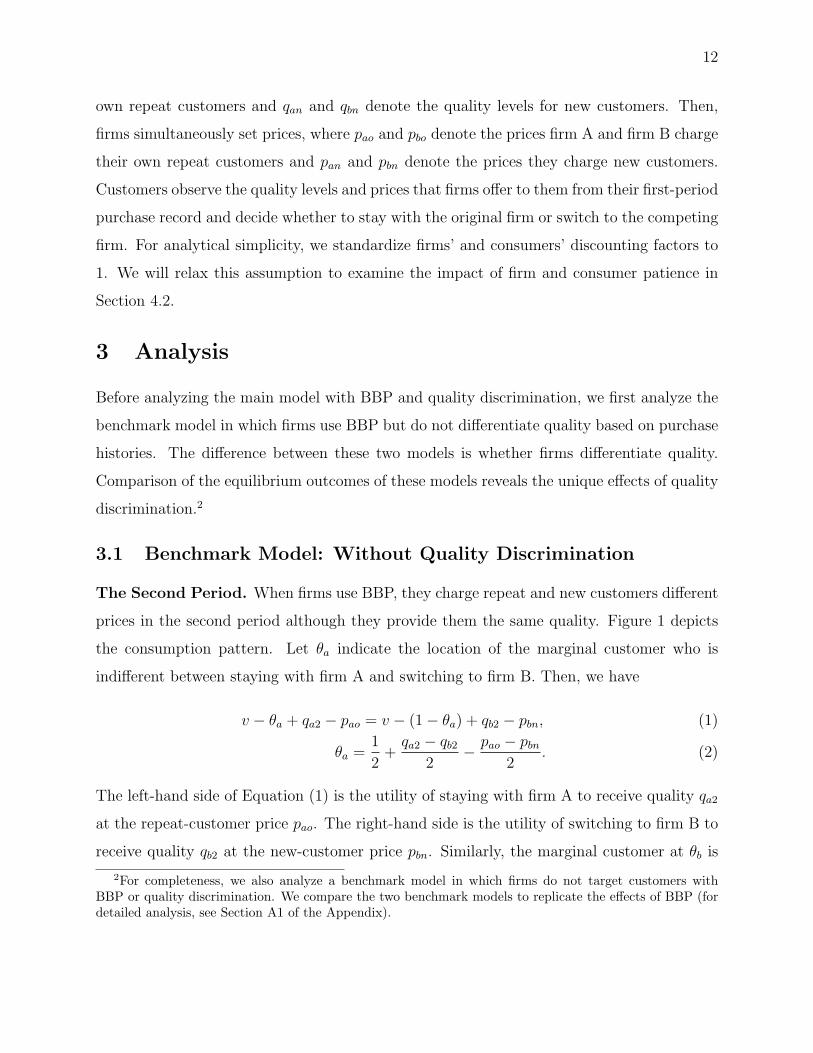
The Second Period. When firms use BBP, they charge repeat and new customers different
prices in the second period although they provide them the same quality. Figure 1 depicts
the consumption pattern. Let θa indicate the location of the marginal customer who is
indifferent between staying with firm A and switching to firm B. Then, we have
v − θa + qa2 − pao = v − (1− θa) + qb2 − pbn, (1)
θa =1
2+
qa2 − qb22
− pao − pbn2
. (2)
The left-hand side of Equation (1) is the utility of staying with firm A to receive quality qa2
at the repeat-customer price pao. The right-hand side is the utility of switching to firm B to
receive quality qb2 at the new-customer price pbn. Similarly, the marginal customer at θb is
2For completeness, we also analyze a benchmark model in which firms do not target customers withBBP or quality discrimination. We compare the two benchmark models to replicate the effects of BBP (fordetailed analysis, see Section A1 of the Appendix).

13
indifferent between switching to firm A and staying with firm B. We therefore write
v − θb + qa2 − pan = v − (1− θb) + qb2 − pbo, (3)
θb =1
2+
qa2 − qb22
− pan − pbo2
. (4)
Firms’ profit functions in the second period are
Πa2 = paoθa + pan(θb − θ1)− (qa2 − qa1)2, (5)
Πb2 = pbo(1− θb) + pbn(θ1 − θa)− (qb2 − qb1)2. (6)
We obtain second-period prices and quality levels using first-order conditions; second-order
conditions are also satisfied. Prices are p∗an = 3−4θ13
+ qa2−qb23
, p∗ao = 1+2θ13
+ qa2−qb23
, p∗bn =
4θ1−13
+ qb2−qa23
, and p∗bo = 3−2θ13
+ qb2−qa23
. Quality levels are q∗a2 = 521
− θ17+ 8qa1−qb1
7and
q∗b2 =221
+ θ17+ 8qb1−qa1
7.
The First Period. The marginal customer at θ1 makes a trade-off between buying from
firm A and firm B in the first period. Anticipating switching firms in the second period, this
customer takes the anticipated second-period utilities into account. We have
v − θ1 + qa1 − pa1 + [v − (1− θ1) + qe∗b2 − pe∗bn] = v − (1− θ1) + qb1 − pb1 + [v − θ1 + qe∗a2 − pe∗an] , (7)
where the superscript e∗ indicates customers’ expectations of the second-period quality and
prices. Assuming rational expectations, we insert the second-period equilibrium quality and
prices into Equation (7) and obtain
θ1 =1
2+
2(qa1 − qb1)
9+
7(pb1 − pa1)
18. (8)
The total profits that firms maximize in the first period are
Πat = pa1θ1 +Π∗a2 − q2a1, (9)
Πbt = pb1(1− θ1) + Π∗b2 − q2b1. (10)
We solve for the first-period equilibrium prices and obtain p∗a1 = 43+ 8(qa1−qb1)
25and p∗b1 =
43+ 8(qb1−qa1)
25. The first-period equilibrium quality levels are q∗a1 = q∗b1 =
1975. We summarize
the rest of the equilibrium outcomes in Table 1.
Next, we analyze the main model with quality discrimination. By comparing the main
model with the benchmark model, we aim to understand how quality discrimination affects
the equilibrium.

14
3.2 Main Model: With Quality Discrimination
Now, consider the case in which firms use consumers’ purchase history data recorded from
the first period to differentiate both quality and prices in the second period. Figure 2 depicts
the consumption pattern.
The Second Period. The marginal customer at θa is indifferent between staying with
firm A and switching to firm B. We can write
v − θa + qao − pao = v − (1− θa) + qbn − pbn, (11)
θa =1
2+
qao − qbn2
− pao − pbn2
. (12)
The left-hand side of Equation (11) is the utility of buying from firm A as a repeat customer.
In this case, the customer receives firm A’s differentiated quality for repeat customers, where
the quality is qao and price is pao. The right-hand side is the utility of switching to firm B. In
this case, the customer receives firm B’s differentiated quality for new customers, where the
quality is qbn and price is pbn. Similarly, the marginal customer at θb is indifferent between
switching to firm A and staying with firm B. We can write
v − θb + qan − pan = v − (1− θb) + qbo − pbo, (13)
θb =1
2+
qan − qbo2
− pan − pbo2
. (14)
The left-hand side of Equation (13) is the utility of switching to firm A, and the right-hand
side is the utility of staying with firm B. Then, firms’ profit functions in the second period
are
Πa2 = paoθa + pan(θb − θ1)− γ[(qao − qa1)
2 + (qan − qa1)2], (15)
Πb2 = pbo(1− θb) + pbn(θ1 − θa)− γ[(qbo − qb1)
2 + (qbn − qb1)2]. (16)
We solve for second-period prices and obtain p∗ao =qao−qbn
3+ 2θ1
3+ 1
3, p∗an = qan−qbo
3− 4θ1
3+ 1,
p∗bo = qbo−qan3
− 2θ13
+ 1, and p∗bn = qbn−qao3
+ 4θ13
− 13. Then, we solve for the second-period
quality and obtain q∗ao = 54γ2qa1−3γ(qa1+qb1)+6γθ1+3γ−θ16γ(9γ−1)
, q∗an = 54γ2qa1−3γ(qa1+qb1)−12γθ1+9γ+θ1−16γ(9γ−1)
,
q∗bo =54γ2qb1−3γ(qa1+qb1)−6γθ1+9γ+θ1−1
6γ(9γ−1), and q∗bn = 54γ2qb1−3γ(qa1+qb1)+12γθ1−3γ−θ1
6γ(9γ−1).
The First Period. In the first period, each firm provides the same quality level of
product features or services to all customers at the same price. The marginal customer

15
at θ1 is indifferent between buying from firm A and firm B in the first period after taking
second-period utilities into account. Thus, we have
v − θ1 + qa1 − pa1 + [v − (1− θ1) + qe∗bn − pe∗bn] = v − (1− θ1) + qb1 − pb1 + [v − θ1 + qe∗an − pe∗an] .(17)
The left-hand side of Equation (17) is the total utility of buying from firm A in the first
period and switching to firm B in the second period. The right-hand side is the total utility
of buying from firm B in the first period and switching to firm A in the second period.
Superscript e∗ indicates consumers’ expectations of the second-period quality and prices
for new customers. Assuming rational expectations, we plug the second-period equilibrium
quality and prices into Equation (17) and obtain
θ1 =1
2− 3γ(9γ − 1)(pa1 − pb1)
(12γ − 1)(6γ − 1)+
3γ(qa1 − qb1)
12γ − 1. (18)
Firms set first-period prices to maximize total profits over two periods. The profit functions
are
Πat = pa1θ1 +Π∗a2 − q2a1, (19)
Πbt = pb1(1− θ1) + Π∗b2 − q2b1. (20)
We solve for first-period prices using first-order conditions and obtain:
p∗a1 =(6γ − 1) [31104γ4 − 17928γ3 + 3330γ2 − 255γ + 7 + (5832γ4 − 2268γ3 + 288γ2 − 12γ)(qa1 − qb1)]
6γ(23328γ4 − 14094γ3 + 2817γ2 − 234γ + 7)
p∗b1 =(6γ − 1) [31104γ4 − 17928γ3 + 3330γ2 − 255γ + 7− (5832γ4 − 2268γ3 + 288γ2 − 12γ)(qa1 − qb1)]
6γ(23328γ4 − 14094γ3 + 2817γ2 − 234γ + 7)
(21)
Using first-order conditions with respect to quality, we obtain:
q∗a1 = q∗b1 =4212γ3 − 2124γ2 + 279γ − 11
6(2592γ3 − 1278γ2 + 171γ − 7)(22)
The second-order conditions are satisfied for γ > 13, i.e., providing quality to a segment of
customers is not too cost efficient than providing quality to all customers. We focus our
analysis on this region of parameter. We illustrate the equilibrium outcomes in Table 1. Let
us understand how firms differentiate quality levels and prices for repeat and new customers
and the resulting implications on profits in the second period.

16
Proposition 1 (The Second Period)
a. Firms provide higher-quality product features or services to repeat customers than to
new customers.
b. Firms charge new customers a lower price than the price they charge repeat customers.
c. Firms’ second-period profits increase with quality discrimination.
The BBP literature shows that in a typical BBP setting, firms reward new customers by
offering them lower prices than what repeat customers pay. This is because new customers
have lower preferences for the firm’s product and buy from the competitor in the first period.
At the same time, firms penalize repeat customers by charging them higher prices than what
new customers pay, because repeat customers have stronger preferences for the firm’s product
than the competitor’s product. Proposition 1 suggests that when firms differentiate quality,
they reward repeat customers on the quality dimension by offering them higher-quality
product features or services than what new customers receive. We also find that when
firms reward repeat customers with higher-quality product features or services, they reward
new customers on the price dimension by offering them a discounted price (see Table 1).
This result is interesting for two reasons. First, it lends new insights to the BBP literature
into whether and how to reward repeat and new customers. Specifically, this result suggests
that managers should reward repeat and new customers with different attributes; that is,
firms should reward new customers with lower prices and reward repeat customers with
a higher quality. Second, this result reveals the (supply-side) difference between quality
discrimination and price discrimination. Consumers’ utility from consumption can be
simplified as quality minus price (i.e., q − p). From the demand side, quality and prices are
perfect substitutes. An increase in price (p) has the same effect on consumers’ utility function
as a decrease in quality (q). Discriminating quality and prices could affect consumers’
purchase decisions the same way. Consequently, rewarding new customers on the price
dimension seems to suggest that firms should also reward new customers on the quality
dimension. Because new customers have lower preferences for the firm’s product, we may
expect the firm to offer higher-quality product features or services to lure the competitor’s
customers to switch firms. However, our result shows that the opposite is true; firms offer
higher-quality product features or services to encourage repeat customers to stay.
17
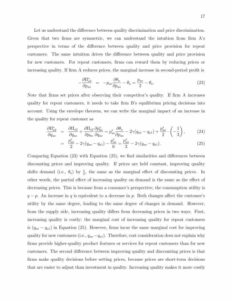
Let us understand the difference between quality discrimination and price discrimination.
Given that two firms are symmetric, we can understand the intuition from firm A’s
perspective in terms of the difference between quality and price provision for repeat
customers. The same intuition drives the difference between quality and price provision
for new customers. For repeat customers, firms can reward them by reducing prices or
increasing quality. If firm A reduces prices, the marginal increase in second-period profit is
−∂Π∗a2
∂pao= −pao
∂θa∂pao
− θa =pao2
− θa. (23)
Note that firms set prices after observing their competitor’s quality. If firm A increases
quality for repeat customers, it needs to take firm B’s equilibrium pricing decisions into
account. Using the envelope theorem, we can write the marginal impact of an increase in
the quality for repeat customer as
∂Π∗a2
∂qao=
∂Πa2
∂qao+
∂Πa2
∂pbn
∂p∗bn∂qao
= p∗ao∂θa∂pao
− 2γ(qao − qa1) +p∗ao2
·(−1
3
), (24)
=p∗ao2
− 2γ(qao − qa1)−p∗ao6
=p∗ao3
− 2γ(qao − qa1). (25)
Comparing Equation (23) with Equation (25), we find similarities and differences between
discounting prices and improving quality. If prices are held constant, improving quality
shifts demand (i.e., θa) by 12, the same as the marginal effect of discounting prices. In
other words, the partial effect of increasing quality on demand is the same as the effect of
decreasing prices. This is because from a consumer’s perspective, the consumption utility is
q − p. An increase in q is equivalent to a decrease in p. Both changes affect the customer’s
utility by the same degree, leading to the same degree of changes in demand. However,
from the supply side, increasing quality differs from decreasing prices in two ways. First,
increasing quality is costly; the marginal cost of increasing quality for repeat customers
is (qao − qa1) in Equation (25). However, firms incur the same marginal cost for improving
quality for new customers (i.e., qan−qa1). Therefore, cost consideration does not explain why
firms provide higher-quality product features or services for repeat customers than for new
customers. The second difference between improving quality and discounting prices is that
firms make quality decisions before setting prices, because prices are short-term decisions
that are easier to adjust than investment in quality. Increasing quality makes it more costly
18
for the competitor to poach the focal firm’s customers. If firm A increases its quality, firm
B must cut prices to attract A’s customers (i.e.,∂p∗bn∂qao
< 0).
Similarly, firms can also increase quality for new customers, which makes it more costly
for the competitor to retain its repeat customers (i.e.,∂p∗bo∂qan
< 0), thereby encouraging firms
to poach each other’s customers. Firms offer higher-quality product features or services to
repeat customers than to new customers, because by doing so, firms make it more appealing
for customers to stay with their original firms and more costly for firms to poach each other’s
customers. As competitive poaching declines, competition becomes softer, and firms’ profits
in the second period increase from the level without quality discrimination. Therefore, this
result of quality discrimination is driven by supply-side considerations. Firms use quality
discrimination as a coordination device to attenuate competitive poaching associated with
price discrimination. This intuition also reflects the difference between quality discrimination
and price discrimination; that is, firms use price discrimination to poach each other’s
customers, which intensifies competition, while they use quality discrimination to alleviate
competitive poaching and soften price competition.
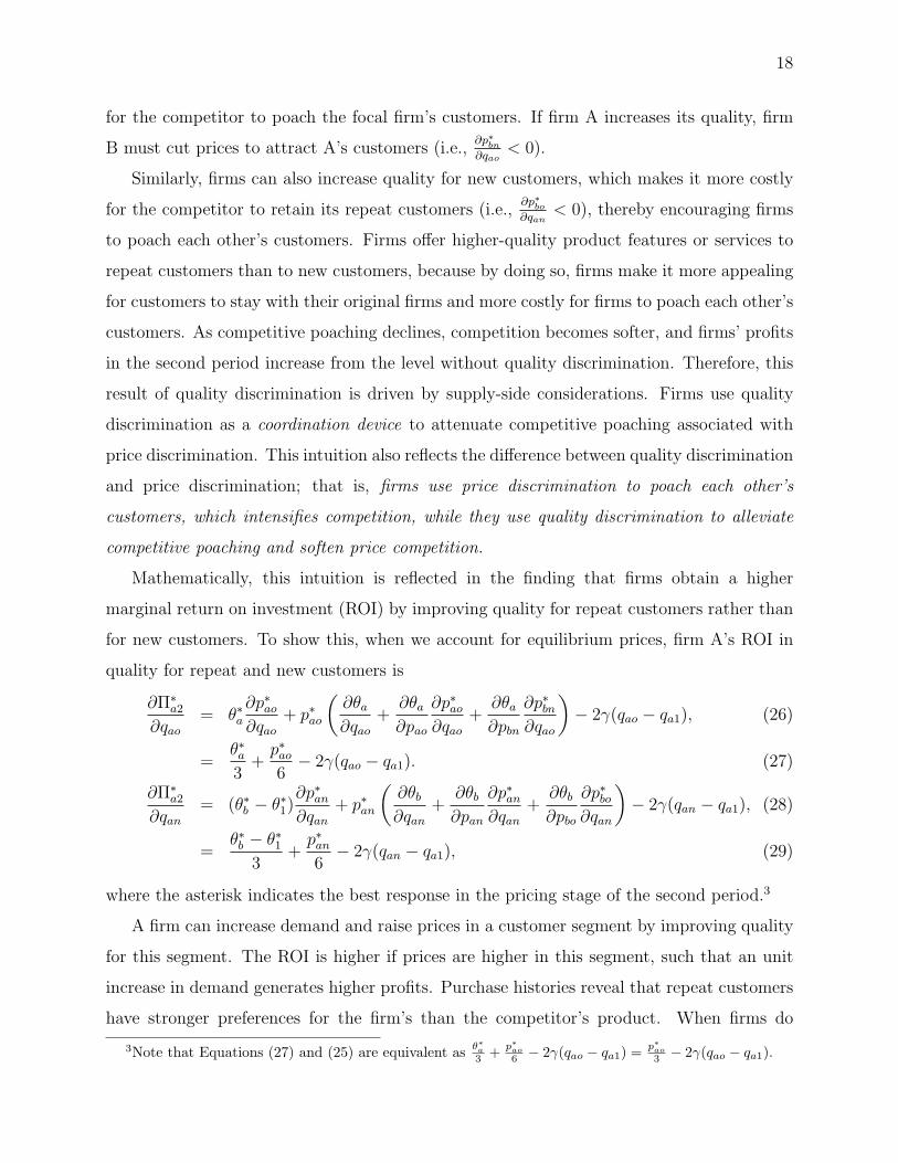
Mathematically, this intuition is reflected in the finding that firms obtain a higher
marginal return on investment (ROI) by improving quality for repeat customers rather than
for new customers. To show this, when we account for equilibrium prices, firm A’s ROI in
quality for repeat and new customers is
∂Π∗a2
∂qao= θ∗a
∂p∗ao∂qao
+ p∗ao
(∂θa∂qao
+∂θa∂pao
∂p∗ao∂qao
+∂θa∂pbn
∂p∗bn∂qao
)− 2γ(qao − qa1), (26)
=θ∗a3
+p∗ao6
− 2γ(qao − qa1). (27)
∂Π∗a2
∂qan= (θ∗b − θ∗1)
∂p∗an∂qan
+ p∗an
(∂θb∂qan
+∂θb∂pan
∂p∗an∂qan
+∂θb∂pbo
∂p∗bo∂qan
)− 2γ(qan − qa1), (28)
=θ∗b − θ∗1
3+
p∗an6
− 2γ(qan − qa1), (29)
where the asterisk indicates the best response in the pricing stage of the second period.3
A firm can increase demand and raise prices in a customer segment by improving quality
for this segment. The ROI is higher if prices are higher in this segment, such that an unit
increase in demand generates higher profits. Purchase histories reveal that repeat customers
have stronger preferences for the firm’s than the competitor’s product. When firms do
3Note that Equations (27) and (25) are equivalent asθ∗a
3 +p∗ao
6 − 2γ(qao − qa1) =p∗ao
3 − 2γ(qao − qa1).
19
not use quality discrimination, they charge higher prices to repeat customers than to new
customers (i.e., p∗ao > p∗an when qao = qan and qbo = qbn). Given the price difference, when
firms use quality discrimination, it is more profitable to invest in quality improvement to
attract repeat customers than new customers. Second, the ROI in quality improvement for
a customer segment is higher if there are more customers in this segment, such that an
increase in price associated with quality improvement generates higher profits. When firms
do not use quality discrimination, they acquire more repeat customers than new customers
(i.e., θ∗a > θ∗b − θ∗1).4 Therefore, when firms use quality discrimination, it is more profitable
to raise prices for repeat customers by improving quality for them. For both these reasons,
firms have stronger incentives to provide higher-quality product features or services to repeat
than new customers.
In general, BBP reduces second-period profits, as competitive poaching intensifies price
competition from the level in the static game (Fudenberg and Tirole 2000). Our results show
that quality discrimination mitigates the traditional BBP’s negative impact on firm profits
in the second period. Note that second-period profits are still lower than those in the static
game without BBP, because quality discrimination does not completely eliminate competitive
poaching associated with BBP. Second-period competition is still more intense than that in
the static game. Therefore, quality discrimination alleviates BBP’s negative impact on
second-period profits. Also note that firms increase repeat-customer prices and reduce
new-customer prices from the levels without quality discrimination. The price difference
between repeat and new customers increases, because firms offer higher-quality product
features or services to repeat customers than to new customers and the quality difference
enlarges the price difference that arises from BBP. Next, let us examine how second-period
quality discrimination affects first-period competition when firms acquire initial customers
and generate purchase history data.
Proposition 2 (The First Period): Quality discrimination leads to lower prices and
profits in the first period.
Proposition 1 shows that quality discrimination benefits firms in the second period. By
contrast, Proposition 2 shows that quality discrimination hurts firms in the first period. The
4θ∗a−(θ∗b −θ∗1) = θ1− 13 +
qao−qan+qbo−qbn6 > 0 when firms do not use quality discrimination (i.e., qao = qan
and qbo = qbn) and θ1 is in the neighborhood of 12 that follows from a symmetric first-period equilibrium.
20
intuition is that quality discrimination increases firms’ ability to retain repeat customers in
the second period, because customers are more willing to stay to enjoy the higher-quality
product features or services for repeat customers. Anticipating this effect of quality
discrimination, forward-looking firms compete aggressively in the first period to build up
their customer base. Thus, firms reduce prices in the first period from the level without
quality discrimination.5
We can show this intuition in detail. Without quality discrimination, forward-looking
firms anticipate that a decrease in first-period prices will expand their first-period market
share. Having a higher market share in the first period will lead a firm’s competitor to
increase second-period quality to poach its customers (i.e.,∂q∗b2∂θ1
> 0), which reduces the
firm’s ability to retain repeat customers, and second-period profit declines accordingly (i.e.,∂Π∗
a2
∂qb2< 0). This dynamic relationship discourages forward-looking firms from reducing
first-period prices to expand the segment of repeat customers. With quality discrimination,
firms are better able to retain repeat customers by offering them higher quality than what
new customers receive. The increase in a firm’s first-period market share induces its
competitor to raise quality for new customers and decrease quality for repeat customers
(i.e.,∂q∗bn∂θ1
> 0 and∂q∗bo∂θ1
< 0). These counteracting effects cancel out and have no impact
on the firm’s second-period profit. Anticipating this effect of quality discrimination, firms
reduce first-period prices and compete more aggressively for initial customers who are more
likely to stay with them to receive the better quality.
This result suggests that though quality discrimination alleviates price competition by
dissuading competitive poaching in the second period, the anticipation of reduced poaching
intensifies first-period competition. These effects of quality discrimination have implications
on firms’ total profits, consumer surplus, and social welfare, which we state in Proposition
3.
Proposition 3 (Overall Welfare): Quality discrimination reduces firms’ total profits but
increases consumer surplus.
Quality discrimination increases profits in the second period and decreases profits more
5Although quality discrimination reduces firms’ prices in the first period, the first-period prices are stillhigher than those in the static game, because consumers are still less price sensitive than they are in thestatic game. Therefore, quality discrimination mitigates the traditional BBP’s impact on consumers’ pricesensitivity in the first period.
21
in the first period. Over the two periods, firms’ total profits are lower with quality
discrimination than without it. BBP research (e.g., Pazgal and Soberman 2008) shows that
when firms simultaneously decide whether to use BBP at the beginning of the first period,
two pure-strategy equilibria exist: both firms do not use BBP or both firms use BBP while
the adoption of BBP is a Pareto dominated equilibrium. However, without commitment
power, firms unilaterally deviate to use BBP at the beginning of the second period, resulting
in lower total profits (i.e., a prisoner’s dilemma). Similarly, our analysis shows that without
credible commitments, firms have incentives to unilaterally deviate to differentiate quality
in the second period. Specifically, if the cost of quality differentiation is low (i.e., γ < 0.55),
firms adopt quality discrimination in the second period. It is profitable for one firm to
differentiate quality. However, when both firms differentiate quality, firms’ total profits
are lower than the profits without quality discrimination, resulting in a prisoner’s dilemma
problem.
With quality discrimination, both prices and quality levels decline in the first period.
The first-period consumer utility increases. In the second period, repeat customers receive
higher-quality product features or services at a higher price, whereas new customers receive
lower-quality product features or services and pay a lower price. Repeat customers’ utility
increases and new customers’ utility decreases. Overall, the first-period effect dominates
and consumer surplus improves with quality discrimination. Social welfare increases when
the cost of quality discrimination is moderate (i.e., γ ∈ (0.35, 0.68)). This is because with
quality discrimination, customers are more willing to stay with their original firms. As a
result, fewer consumers make inefficient switching between firms and social welfare increases
with quality discrimination.
4 Extensions
In this section, we relax several assumptions made in the main model to show the robustness
of the main results. In Section 4.1, we relax the assumption on the cost functions to generalize
our results. In Section 4.2, we allow firms and consumers to discount the future payoff. In
Section 4.3, we incorporate consumers’ switching costs into the analysis. We summarize key
findings below and show detailed analyses in the Appendix.

22
4.1 Alternative Cost Functions
In the main model, we assumed that firms incur costs to improve quality in the second period.
Without further investment, second-period quality level does not reinitialize to zero. Here,
we examine whether our key findings are robust to this assumption. Assume that quality
reinitializes to zero and firms’ cost function for providing quality qi2 in the second period is
C(qi2) = q2i2 rather than C(qi2) = (qi2 − qi1)2. As a result, when firms differentiate quality,
their second-period profit functions become Πa2 = paoθa+pan(θb−θ1)−γ (q2ao + q2an) and Πb2 =
pbo(1−θb)+pbn(θ1−θa)−γ (q2bo + q2bn). We solve the benchmark and main models and verify
that all results in the main model hold (see Table 2). That is, firms provide higher-quality
product features or services to repeat customers than to new customers, whereas firms charge
new customers lower prices. First-period prices decline. Second-period profits increase while
first-period profits decline. Total profits are lower with quality discrimination (for detailed
analysis, see Section A2 in the Appendix). When second-period quality reinitializes to zero,
second-period quality levels decline. This is intuitive because providing high-quality product
features or services in the second period becomes more costly under the new assumption.
Moreover, when second-period quality reinitializes to zero, an increase in first-period
quality does not make quality provision in the second period less costly. The investment
in first-period quality only helps the firm to compete for customers in the first period
rather than both periods. We would expect firms to have lower incentives to invest in
quality provision in the first period if the quality does not carry into the second period.
Interestingly, we find that first-period quality increases if second-period quality reinitializes
to zero. The intuition is as follows. Suppose that firm A increases its first-period quality
(qa1) and second-period quality does not reinitializes. Consumers anticipate that firm
A’s second-period quality will also increase accordingly as firm A only invests in quality
improvement from the level of qa1 in the second period. Since the first-period marginal
customer switches firms, he or she has incentives to buy from firm B in the first period to
enjoy firm A’s higher-quality product features or services in the second period after switching
firms. Consumers’ second-period consideration leads first-period demand to decrease with
first-period quality (i.e.,∂θ∗1∂qa1
= − 9166
). Therefore, firms provide lower-quality product
features or services in the first period to expand demand. By contrast, when quality
reinitializes to zero in the second period, an increase in first-period quality does not affect
23
second-period quality. First-period consumers are more willing to buy from the firm that
provides higher quality in the first period and demand increases with first-period quality
(i.e.,∂θ∗1∂qa1
= 441664
). Therefore, firms provide higher-quality product features or services in the
first period than they would if quality carries into the second period.
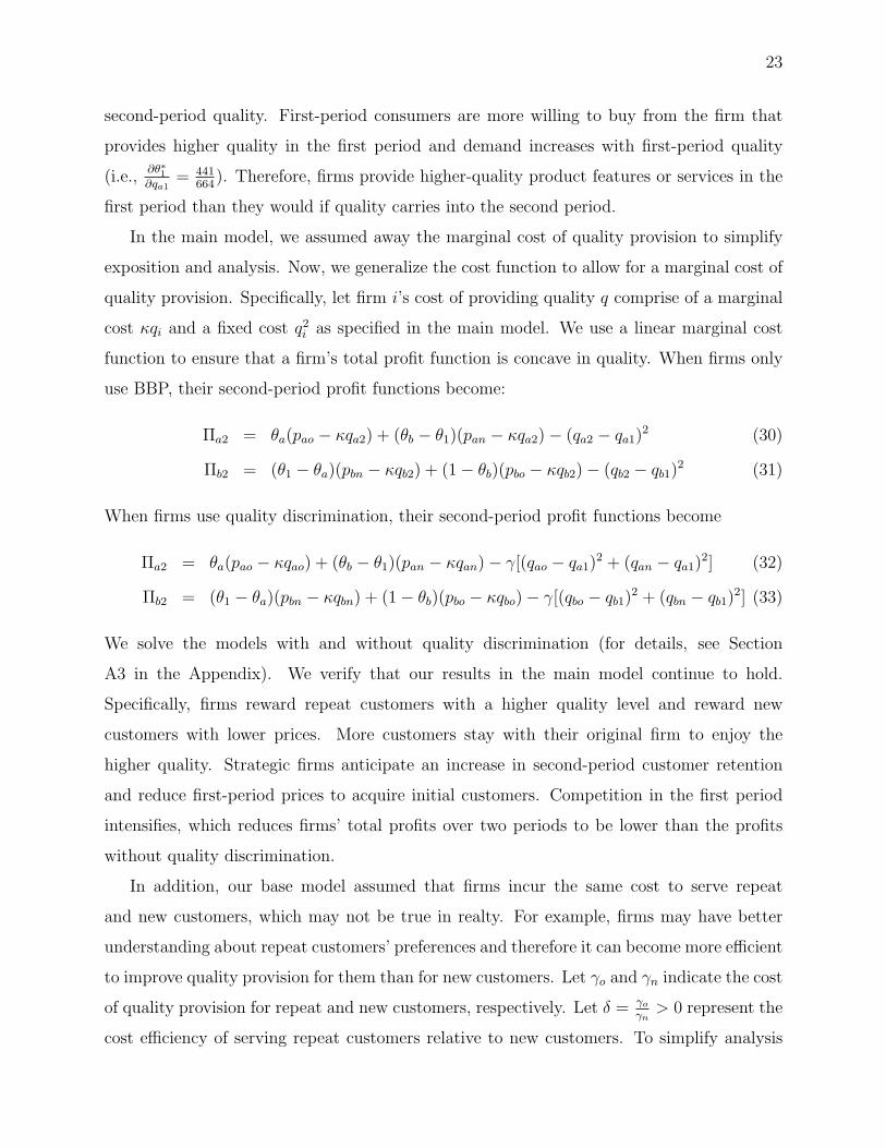
In the main model, we assumed away the marginal cost of quality provision to simplify
exposition and analysis. Now, we generalize the cost function to allow for a marginal cost of
quality provision. Specifically, let firm i’s cost of providing quality q comprise of a marginal
cost κqi and a fixed cost q2i as specified in the main model. We use a linear marginal cost
function to ensure that a firm’s total profit function is concave in quality. When firms only
use BBP, their second-period profit functions become:
Πa2 = θa(pao − κqa2) + (θb − θ1)(pan − κqa2)− (qa2 − qa1)2 (30)
Πb2 = (θ1 − θa)(pbn − κqb2) + (1− θb)(pbo − κqb2)− (qb2 − qb1)2 (31)
When firms use quality discrimination, their second-period profit functions become
Πa2 = θa(pao − κqao) + (θb − θ1)(pan − κqan)− γ[(qao − qa1)2 + (qan − qa1)
2] (32)
Πb2 = (θ1 − θa)(pbn − κqbn) + (1− θb)(pbo − κqbo)− γ[(qbo − qb1)2 + (qbn − qb1)
2] (33)
We solve the models with and without quality discrimination (for details, see Section
A3 in the Appendix). We verify that our results in the main model continue to hold.
Specifically, firms reward repeat customers with a higher quality level and reward new
customers with lower prices. More customers stay with their original firm to enjoy the
higher quality. Strategic firms anticipate an increase in second-period customer retention
and reduce first-period prices to acquire initial customers. Competition in the first period
intensifies, which reduces firms’ total profits over two periods to be lower than the profits
without quality discrimination.
In addition, our base model assumed that firms incur the same cost to serve repeat
and new customers, which may not be true in realty. For example, firms may have better
understanding about repeat customers’ preferences and therefore it can become more efficient
to improve quality provision for them than for new customers. Let γo and γn indicate the cost
of quality provision for repeat and new customers, respectively. Let δ = γoγn
> 0 represent the
cost efficiency of serving repeat customers relative to new customers. To simplify analysis
24
and exposition, we assume that the second-period quality reinitializes to zero. We solve
the equilibrium as in the main model (for details, please see the Appendix). Proposition 4
summarizes our new findings. We focus on situations when the cost of serving customers is
not negligible (i.e., γn, γo >112).
Proposition 4 As serving repeat customers becomes more costly relative to serving new
customers (i.e., δ increases), firms’ second-period profits decrease, first-period profits
increase, and total profits increase.
Our analysis yields several interesting findings. First, we find that as long as serving
repeat customers is not twice more costly than serving new customers (i.e., δ < 2), firms still
provide a higher quality level to repeat customers than to new customers (i.e., q∗ao > q∗an).
In this case, firms still reward new customers with a discounted price (i.e., p∗ao > p∗an).
Second, intuitively, as δ increases, it becomes relatively more costly to serve repeat customers
than new customers. Thus, firms reduce quality provision for repeat customers and increase
quality provision for new customers. Third, our analysis shows that as it becomes more costly
to serve repeat customers than new customers (i.e., δ increases), firms’ second-period profits
decline. This is because cost inefficiency of serving repeat than new customers constrained
firm’s ability to use quality discrimination to deter competitive poaching and soften price
competition. Firms’ second-period profits decline accordingly. Fourth, we also find that
firm’s first-period profits increase with δ. This is because as δ increases, it becomes more
costly to perform behavior-based quality discrimination in the second period as providing a
higher quality to repeat customers becomes relatively more costly. As firms reduce quality
discrimination in the second period, customer retention decreases. Anticipating this, firms
in the first period have less incentives to cut prices to acquire initial customers. Therefore,
profits in the first period increase. Lastly, as δ increases, firms become less engaged in the
behavior-based quality discrimination that reduces total profits. As a result, a higher cost
of serving repeat customers than new customers serves as a commitment device for firms to
reduce quality discrimination and increase total profits.
25
4.2 Firm and Consumer Patience
In our main model, we assumed that firms and consumers did not discount the second-period
payoff. This assumption is plausible when the time distance between the two periods is short.
Given that some of the results in our main model arise from firms’ and consumers’ strategic
forward-looking behavior, we relax the main model to consider how firm and consumer
patience (i.e., their discounting factor) may affect our results. To simplify analysis, we set
γ = 12. Let δf , δc ∈ [0, 1] represent firms’ and consumers’ discount factor, respectively. A
higher value means that firms or consumers are more forward-looking or patient so that the
future utility weighs more heavily in their first-period decision making. Given that firm and
consumer patience only affects first-period decisions, results pertaining to the second-period
outcomes in Proposition 1 continue to hold.
Proposition 5 When firms only use BBP, firm and consumer patience increases first-period
prices. When firms use BBP and quality discrimination, consumer patience decreases
first-period prices.
Proposition 5 reflects the opposite effects of firm and consumer patience on firms’ first-period
pricing decisions. When firms only use BBP, as firms and consumer become more patient,
firms raise first-period prices. This is because consumers are willing to pay a higher price
in the first period when they anticipate receiving a better deal in the second period. This
forward-looking behavior leads first-period demand to become less price sensitive and results
in a higher first-period price. This effect becomes stronger when consumers are more
patient. Therefore, consumer patience increases first-period prices. At the same time,
when firms use BBP, their first-period market share reduces their second-period profit. This
is because as a firm obtains a larger market share from the first-period competition, its
competitor will increase second-period quality level to attract its customers, which reduces
its second-period profit. Anticipating this effect, firms strategically raise first-period prices
to reduce first-period market share and increase second-period profit. The more patient
firms are, the higher they raise first-period prices for the second-period benefit. Therefore,
as firms become more patient, their first-period prices increase.
However, when firms also differentiate quality for the two segments of repeat and new
customers, the effect of consumer patience flips and the effect of firm patience no longer exists.
26
Consumer patience reduces first-period prices because consumers anticipate less willingness
to switch in the second period because firms reward repeat customers. This anticipation
makes consumers more price sensitive in the first period. Therefore, consumer patience
increases consumers’ price sensitivity and reduces prices in the first period. Firm patience
no longer has impact on first-period pricing, because as a firm expands its first-period
market share, its competitor provides higher-quality product features or services for new
customers and lower-quality product features or services for repeat customers. These
counteracting changes in second-period quality levels result in no impact on second-period
profits. Therefore, firms’ forward-looking behavior has no impact on their first-period prices.
When firms and consumers are myopic (i.e., δf = δc = 0), the game reduces to the static
game without behavior-based targeting. In this case, prices and firm profits are the same
with or without quality differentiation. when firms and consumers are somewhat patient
(i.e., δf > 0 and δc > 0), Proposition 5 suggests that first-period prices would be lower with
quality differentiation. Consequently, first-period profits decline with quality differentiation,
which leads firms’ profits to be lower with quality differentiation than without it. Thus, our
results pertaining to the first-period prices and profits as well as the total profits and welfare
continue to hold.
4.3 Switching Costs
When consumers switch firms in the second period, they may incur switching costs. The
switching costs could arise from physical learning costs or psychological factors such as
inertia (Klemperer 1987, 1995, Farrell and Klemperer 2007). Let s denote switching costs.
If switching costs are prohibitive, no consumers switch firms. Thus, we focus our analysis
on the case when s < 23, such that both firms poach competitors’ customers when they use
BBP and quality discrimination and consumers switch firms in equilibrium. We solve the
benchmark and main models and present the equilibrium outcomes in Table 3.
Our analysis shows that switching costs enhance the key results that we present in
the main model. Specifically, with switching costs, firms increase quality level for repeat
customers and decrease quality level for new customers. This result is counterintuitive
because repeat customers are locked in with their firm, which seems to suggest that firms
do not have incentives to provide higher-quality product features or services to them. The

27
reason is that when repeat customers face a higher switching cost, it is harder for firms to
poach their competitor’s customers. As a result, firms offer lower prices to poach customers,
which makes competitive poaching more harmful for firms. Firms have greater incentives
to attenuate competitive poaching by securing their repeat customers with an even higher
quality level. Thus, firms continue to reward repeat (new) customers on the quality (price)
dimension and the quality (price) difference increases with switching costs.
Switching costs lead firms to reduce prices in the first period to attract customers as
customers will be locked in with them in the second period. Firms exploit the switching
costs by raising prices for repeat customers and second-period profits increase. However,
first-period profits decrease more and firms’ total profits decline with switching costs. In
addition, when switching costs are sufficiently high, firms have incentives to raise first-period
prices to depress their first-period market share, so that the competitor does not poach its
customers in the second period. Even in this scenario, our key results presented in the
propositions continue to hold (for detailed analysis, see Section A4 in the Appendix).
5 Conclusion
New information technology makes it possible for firms to differentiate quality and prices
for repeat and new customers. Firms’ practice of behavior-based quality discrimination has
become increasingly common in various industries. Existing research has focused on firms’
pricing decisions and established the effects of BBP (Fudenberg and Villas-Boas 2006). The
current research contributes to the BBP literature by allowing firms to differentiate both
quality and prices on the basis of purchase histories and examining the unique effects of
behavior-based quality discrimination. Our key findings address the research questions we
initially posited and, in turn, provide theoretical and managerial insights.
Should firms reward new customers or repeat customers? Our analysis suggests that
the answer to this question is not simply determining which types of customers should
receive rewards. Instead, firms should reward different types of customers with different
attributes. Specifically, our results show that firms should reward repeat customers on the
quality dimension by providing them higher-quality product features or services. At the
same time, firms should reward new customers on the price dimension by offering them a
28
switching discount. Therefore, firms should provide the right reward to the right type of
customers.
What is the fundamental difference between quality discrimination and price
discrimination? Our analysis reveals that quality discrimination and price discrimination
have two main differences. First, quality discrimination is costly. Second, firms make
quality decisions before making pricing decisions. By quality discrimination and rewarding
repeat customers with better quality, firms reduce competitive poaching. Thus, quality
discrimination is a coordination device that alleviates competition associated with price
discrimination in the second period.
How should firms adjust first-period prices to compete for initial customers? Our
results show that forward-looking firms anticipate higher customer retention with quality
discrimination. Such anticipation leads firms to reduce prices in the first period to
aggressively compete for initial customers and build up customer base.
How does quality discrimination affect firm profits, consumer surplus, and social welfare?
We find that quality discrimination alleviates competitive poaching in the second period and
increases second-period profits. However, quality discrimination intensifies price competition
in the first period and decreases first-period profits. Firms’ total profits decline, though
consumer surplus and social welfare tend to improve with quality discrimination.
This article provides several directions for future research. First, we focused on firms’
behavior-based quality decisions. Future research could examine how firms differentiate other
important strategies on the basis of consumers’ purchase histories to glean qualitatively new
insights. Second, firms have begun using big data to improve their decisions. Thus, it would
be worthwhile to examine how firms use other types of consumer data and the resultant
implications on firm profits, consumer surplus, and social welfare. Third, this article reveals
the theoretical insights that firms should reward repeat customers on the quality dimension
and reward new customers on the price dimension. Future research could empirically examine
how firms’ practice of quality and price discrimination between repeat and new customers
affects firm profits and financial performance.
29
References
Acquisti, A. and H. R. Varian (2005), “Conditioning Prices on Purchase History,” MarketingScience, 24, 3, 367-381.
Chen, Y. (1997), “Paying Customers to Switch,” Journal of Economics & ManagementStrategy, 6, 4, 877-897.
Chen, Y. and G. Iyer (2002), “Consumer Addressability and Customized Pricing,”MarketingScience, 21, 2, 197-208.
Delta (2018), “Delta Sky Club News & Updates,” available at https://www.
delta.com/content/www/en_US/traveling-with-us/airports-and-aircraft/
delta-sky-club/news-and-updates.html.
Farrell, J. and P. Klemperer (2007), “Coordination and Lock-In: Competition with SwitchingCosts and Network Effects,” Handbook of Industrial Organization, edition 1, volume 3,number 1, Elsevier.
Fudenberg, D. and J. Tirole (2000), “Customer Poaching and Firm Switching,” The RANDJournal of Economics, 31, 4, 634-657.
Fudenberg, D. and J. M. Villas-Boas (2006), “Behavior-Based Price Discrimination andCustomer Recognition,” Handbook on Economics and Information Systems, 377-436, T.J.Hendershott, Ed., Elsevier.
Klemperer, P. (1987), “The Competitiveness of Markets with Switching Costs,” Rand Journalof Economics, 18, 1, 138-150.
Klemperer, P. (1995), “Competition When Consumers Have Switching Costs: An Overviewwith Applications to Industrial Organization, Macroeconomics and International Trade,”Review of Economics Studies, 62, 515-539.
Lewis, M. (2004), “The Influence of Loyalty Programs and Short-Term Promotions onCustomer Retention,” Journal of Marketing Research, 41, 281-292.
Pazgal, A. and D. Soberman (2008), “Behavior-Based Discrimination: Is it a Winning Play,and If So, When?” Marketing Science, 27, 6, 977-994.
Rhee, K.-E. and R. Thomadsen (2016), “Behavior-Based Pricing in Vertically DifferentiatedIndustries,” Management Science, forthcoming.
Shaffer, G. and Z. J. Zhang (2000), “Preference-Based Price Discrimination in Markets withSwitching Costs,” Journal of Economics and Management Strategy, 9, 3, 397-424.
Shen, Q. and J. M. Villas-Boas (2017), “Behavior-Based Advertising,” Management Science,Articles in Advance, 1-18.
Shin, J. and K. Sudhir (2010), “A Customer Management Dilemma: When Is It Profitableto Reward One’s Own Customers?” Marketing Science, 29, 4, 671-689.
Shin, J., K. Sudhir, and D.-H. Yoon (2012), “When to “Fire” Customers: CustomerCost-Based Pricing,” Management Science, 58, 5, 932-947.
30
Subramanian, U., J. S. Raju, Z. J. Zhang (2014), “The Strategic Value of High-CostCustomers,” Management Science, 60, 2, 494-507.
Techbargains (2018), “Amazon Prime: Free 30-Day Trial, $20 off First TimeMembers w/ Echo,” available at https://www.techbargains.com/deal/387638/
amazon-prime-deals.
Villas-Boas, J. M. (1999), “Dynamic Competition with Customer Recognition,” RANDJournal of Economics, 30, 4, 604-631.
Villas-Boas, J. M. (2004), “Price Cycles in Markets with Customer Recognition,” RANDJournal of Economics, 35, 3, 486-501.
Zhang, J. (2011), “The Perils of Behavior-Based Personalization,” Marketing Science, 30, 1,170-186.

31
Table 1: Equilibrium Outcomes (γ = 12)
Benchmark Model Main ModelSecond-Period Quality q∗a2: 0.420 q∗ao: 0.487
q∗an: 0.344First-Period Quality q∗a1: 0.253 q∗a1: 0.249Second-Period Prices p∗ao: 0.667 p∗ao: 0.714
p∗an: 0.333 p∗an: 0.286First-Period Prices p∗a1: 1.333 p∗a1: 0.952Second-Period Profits (Π∗
a2) 0.250 0.263First-Period Profits (Π∗
a1) 0.602 0.414Total Profits (Π∗
at) 0.852 0.677Consumer Surplus (CS∗) 18.229 18.610Social Welfare (SW ∗) 19.934 19.965
Table 2: Equilibrium Outcomes when Second-Period Quality Reinitializes to Zero (γ = 12)
Benchmark Model Main ModelSecond-Period Quality q∗a2: 0.167 q∗ao: 0.238
q∗an: 0.095First-Period Quality q∗a1: 0.230 q∗a1: 0.283Second-Period Prices p∗ao: 0.667 p∗ao: 0.714
p∗an: 0.333 p∗an: 0.286First-Period Prices p∗a1: 1.333 p∗a1: 0.952Second-Period Profits (Π∗
a2) 0.250 0.263First-Period Profits (Π∗
a1) 0.614 0.396Total Profits (Π∗
at) 0.864 0.659Consumer Surplus (CS∗) 17.952 18.395Social Welfare (SW ∗) 19.680 19.714
Table 3: Equilibrium Outcomes with Switching Costs (γ = 12)
Benchmark Model Main ModelSecond-Period Quality q∗a2: 0.420 q∗ao: 0.487 + 0.143s
q∗an: 0.344− 0.143sFirst-Period Quality q∗a1: 0.253 q∗a1: 0.249Second-Period Prices p∗ao: 0.667 + 0.333s p∗ao: 0.714 + 0.429s
p∗an: 0.333− 0.333s p∗an: 0.286− 0.429sFirst-Period Prices p∗a1: 1.333− 0.667s p∗a1: 0.952− 0.762sSecond-Period Profits (Π∗
a2) 0.250 + 0.111s+ 0.111s2 0.263 + 0.163s+ 0.163s2
First-Period Profits (Π∗a1) 0.602− 0.333s 0.414− 0.381s
Total Profits (Π∗at) 0.852− 0.222s+ 0.111s2 0.677− 0.218s+ 0.163s2
Consumer Surplus (CS∗) 18.229 + 0.222s+ 0.056s2 18.610 + 0.354s+ 0.092s2
Social Welfare (SW ∗) 19.934− 0.222s+ 0.278s2 19.965− 0.082s+ 0.418s2

32
Figure 1: Benchmark Model: Without Quality Discrimination
•0
•θ1
|Buy from A (qa1, pa1) Buy from B (qb1, pb1)•1
Period 1
•0
•θa
|Stay with A
(qa2, pao) •θ1
|Switch to B
(qb2, pbn) •θb
|Switch to A(qa2, pan) •
1
Stay with B(qb2, pbo)
Period 2
Figure 2: Main Model: With Quality Discrimination
•0
•θ1
|Buy from A (qa1, pa1) Buy from B (qb1, pb1)•1
Period 1
•0
•θa
|Stay with A(qao, pao) •
θ1
|Switch to B
(qbn, pbn) •θb
|Switch to A(qan, pan) •
1
Stay with B(qbo, pbo)
Period 2

A1
Technical Appendix
Proof of Proposition 1
When firms adopt quality discrimination, second-period equilibrium quality levels are:
q∗ao =75816γ5 − 15552γ4 − 8658γ3 + 2574γ2 − 233γ + 7
12(9γ − 1)γ(2592γ3 − 1278γ2 + 171γ − 7)(A1)
q∗an =75816γ5 − 31104γ4 − 990γ3 + 1548γ2 − 191γ + 7)
12(9γ − 1)γ(2592γ3 − 1278γ2 + 171γ − 7)(A2)
It follows that q∗ao − q∗an = 12(9γ−1)
> 0 for γ > 13, the region that we consider. Therefore,
firms reward repeat customers on the quality dimension. Second-period equilibrium pricesare:
p∗ao =12γ − 1
2(9γ − 1)(A3)
p∗an =6γ − 1
2(9γ − 1)(A4)
We can obtain that p∗ao − p∗an = 3γ9γ−1
> 0 for γ > 13, the region that we consider. Therefore,
firms reward new customers on the price dimension. The second-period equilibrium profitsare
Π∗a2 = Π∗
b2 =(18γ − 1)(90γ2 − 18γ + 1)
72γ(9γ − 1)2(A5)
which is higher than the second-period profit (i.e., 14) without quality differentiation.
Proof of Proposition 2
When firms adopt quality discrimination, first-period prices are
p∗a1 =(12γ − 1)(6γ − 1)
6γ(9γ − 1)(A6)
which is lower than the first-period price (43) without quality customization when γ > 1
3.
First-period profits are
Π∗a1 =
U1
36γ(9γ − 1)(2592γ3 − 1278γ2 + 171γ − 7)2(A7)
where U1 = 1291519728γ8 − 1615055760γ7 + 842531544γ6 − 239826096γ5 + 40902651γ4 −4302567γ3+274032γ2−9707γ+147. The profits are lower than the first-period profits (3389
5625)
without quality customization.

A2
Proof of Proposition 3
Let superscript PP and CC indicate the models with BBP only and with qualitydiscrimination. We compare firms’ total profits over two periods, consumer surplus, andsocial welfare between these two cases.
Π∗CCat − Π∗PP
at =U2
72(9γ − 1)2γ(2592γ3 − 1278γ2 + 171γ − 7)2− 19181
22500(A8)
where U2 = 34131266784γ9 − 45168233472γ8 + 25462348704γ7 − 8057182104γ6 +1585564146γ5 − 202203702γ4 +16778358γ3 − 876393γ2 +26218γ− 343. The above equationis negative for γ > 1
3, the region we consider. Therefore, quality discrimination decreases
firm’s total profits over two periods.
CS∗CCat = 2
∫ θ∗a
0
(v + q∗a1 − θ − p∗a1 + v + q∗a2 − θ − p∗ao)dθ
+2
∫ θ∗1
θ∗a
(v + q∗a1 − θ − p∗a1 + v + q∗b2 − 1 + θ − p∗bn)dθ
= 2v − 9587808γ6 − 8195904γ5 + 2759832γ4 − 473922γ3 + 44181γ2 − 2135γ + 42
24γ(9γ − 1)2(2592γ3 − 1278γ2 + 171γ − 7)
CS∗PPat = 2
∫ θ∗a
0
(v + q∗a1 − θ − p∗a1 + v + q∗ao − θ − p∗ao)dθ
+2
∫ θ∗1
θ∗a
(v + q∗a1 − θ − p∗a1 + v + q∗bn − 1 + θ − p∗bn)dθ
= 2v − 797
450(A9)
CS∗CCat − CS∗PP
at =U3
1800γ(9γ − 1)2(2592γ3 − 1278γ2 + 171γ − 7)> 0 (A10)
for γ > 13, where U3 = −(49758624γ6−135938088γ5+81230364γ4−19849626γ3+2366739γ2−
137809γ + 3150). Therefore, quality discrimination increases consumer surplus.
SW ∗CCat = CS∗CC
at +Π∗CCat = 2v − U4
72γ(9γ − 1)2(2592γ3 − 1278γ2 + 171γ − 7)2
SW ∗PPat = CS∗PP
at +Π∗PPat = 2v − 124
1875(A11)
where U4 = 6292261440γ9−10154538432γ8+6877397664γ7−2557891872γ6+577347912γ5−82662768γ4 + 7572681γ3 − 431298γ2 + 13945γ − 196.
SW ∗CCat − SW ∗PP
at = − U5
45000(9γ − 1)2γ(2592γ3 − 1278γ2 + 171γ − 7)2(A12)
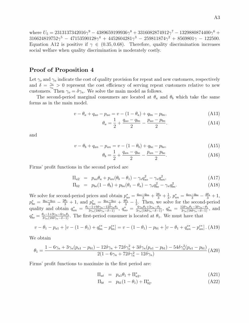
A3
where U5 = 2313137342016γ9 − 4389659199936γ8 + 3316082874912γ7 − 1329880874400γ6 +316624819752γ5 − 47153590128γ4 + 4452604281γ3 − 259811874γ2 + 8569801γ − 122500.Equation A12 is positive if γ ∈ (0.35, 0.68). Therefore, quality discrimination increasessocial welfare when quality discrimination is moderately costly.
Proof of Proposition 4
Let γo and γn indicate the cost of quality provision for repeat and new customers, respectivelyand δ = γo
γn> 0 represent the cost efficiency of serving repeat customers relative to new
customers. Then γo = δγn. We solve the main model as follows.The second-period marginal consumers are located at θa and θb which take the same
forms as in the main model.
v − θa + qao − pao = v − (1− θa) + qbn − pbn, (A13)
θa =1
2+
qao − qbn2
− pao − pbn2
. (A14)
and
v − θb + qan − pan = v − (1− θb) + qbo − pbo, (A15)
θb =1
2+
qan − qbo2
− pan − pbo2
. (A16)
Firms’ profit functions in the second period are
Πa2 = paoθa + pan(θb − θ1)− γoq2ao − γnq
2an, (A17)
Πb2 = pbo(1− θb) + pbn(θ1 − θa)− γoq2bo − γnq
2bn. (A18)
We solve for second-period prices and obtain p∗ao =qao−qbn
3+ 2θ1
3+ 1
3, p∗an = qan−qbo
3− 4θ1
3+ 1,
p∗bo = qbo−qan3
− 2θ13
+ 1, and p∗bn = qbn−qao3
+ 4θ13
− 13. Then, we solve for the second-period
quality and obtain q∗an = θ1−1+9δγn−12δγnθ13γn(18δγn−δ−1)
, q∗ao = 6γnθ1+3γn−θ13γn(18δγn−δ−1)
, q∗bn = 12δγnθ1−3δγn−θ13γn(18δγn−δ−1)
, and
q∗bo =θ1−1+9γn−6γnθ13γn(18δγn−δ−1)
. The first-period consumer is located at θ1. We must have that
v − θ1 − pa1 + [v − (1− θ1) + qe∗bn − pe∗bn] = v − (1− θ1)− pb1 + [v − θ1 + qe∗an − pe∗an] . (A19)
We obtain
θ1 =1− 6γn + 3γn(pa1 − pb1)− 12δγn + 72δγ2
n + 3δγn(pa1 − pb1)− 54δγ2n(pa1 − pb1)
2(1− 6γn + 72δγ2n − 12δγn)
(A20)
Firms’ profit functions to maximize in the first period are:
Πat = pa1θ1 +Π∗a2, (A21)
Πbt = pb1(1− θ1) + Π∗b2. (A22)
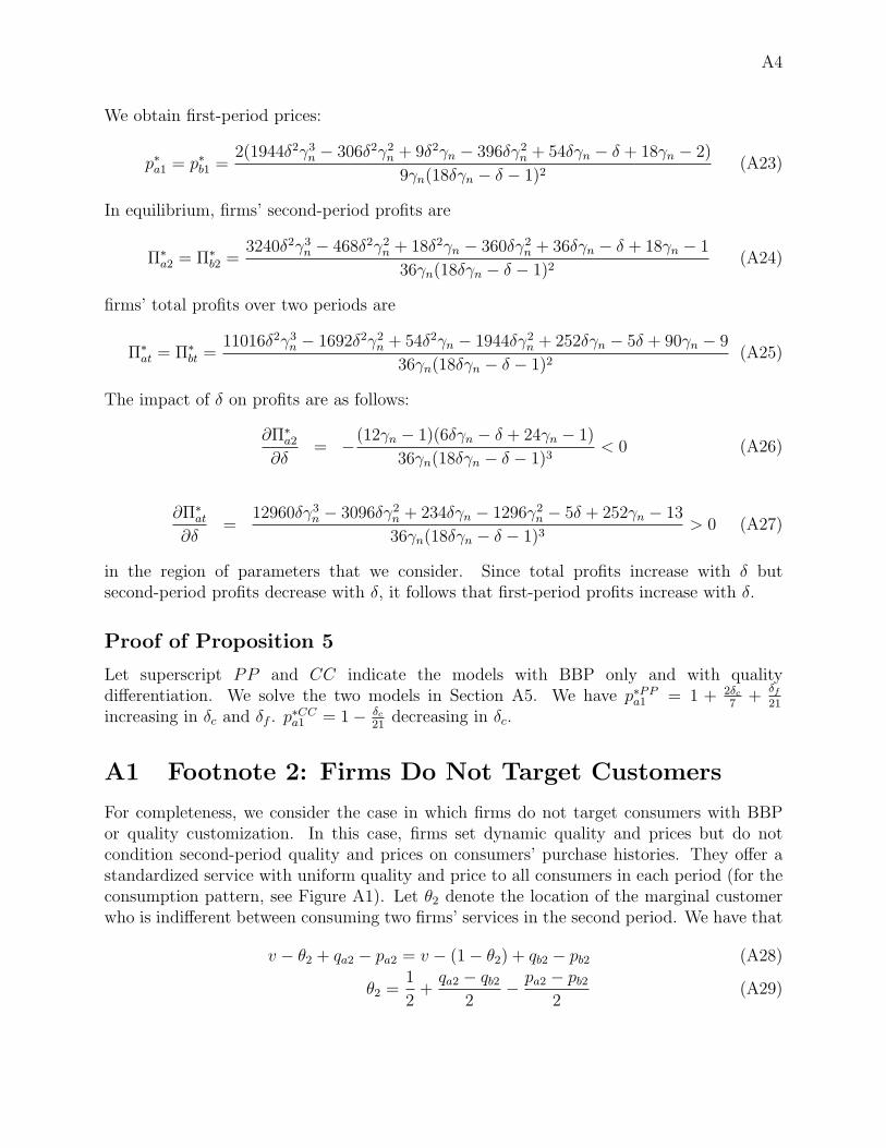
A4
We obtain first-period prices:
p∗a1 = p∗b1 =2(1944δ2γ3
n − 306δ2γ2n + 9δ2γn − 396δγ2
n + 54δγn − δ + 18γn − 2)
9γn(18δγn − δ − 1)2(A23)
In equilibrium, firms’ second-period profits are
Π∗a2 = Π∗
b2 =3240δ2γ3
n − 468δ2γ2n + 18δ2γn − 360δγ2
n + 36δγn − δ + 18γn − 1
36γn(18δγn − δ − 1)2(A24)
firms’ total profits over two periods are
Π∗at = Π∗
bt =11016δ2γ3
n − 1692δ2γ2n + 54δ2γn − 1944δγ2
n + 252δγn − 5δ + 90γn − 9
36γn(18δγn − δ − 1)2(A25)
The impact of δ on profits are as follows:
∂Π∗a2
∂δ= −(12γn − 1)(6δγn − δ + 24γn − 1)
36γn(18δγn − δ − 1)3< 0 (A26)
∂Π∗at
∂δ=
12960δγ3n − 3096δγ2
n + 234δγn − 1296γ2n − 5δ + 252γn − 13
36γn(18δγn − δ − 1)3> 0 (A27)
in the region of parameters that we consider. Since total profits increase with δ butsecond-period profits decrease with δ, it follows that first-period profits increase with δ.
Proof of Proposition 5
Let superscript PP and CC indicate the models with BBP only and with qualitydifferentiation. We solve the two models in Section A5. We have p∗PP
a1 = 1 + 2δc7
+δf21
increasing in δc and δf . p∗CCa1 = 1− δc
21decreasing in δc.
A1 Footnote 2: Firms Do Not Target Customers
For completeness, we consider the case in which firms do not target consumers with BBPor quality customization. In this case, firms set dynamic quality and prices but do notcondition second-period quality and prices on consumers’ purchase histories. They offer astandardized service with uniform quality and price to all consumers in each period (for theconsumption pattern, see Figure A1). Let θ2 denote the location of the marginal customerwho is indifferent between consuming two firms’ services in the second period. We have that
v − θ2 + qa2 − pa2 = v − (1− θ2) + qb2 − pb2 (A28)
θ2 =1
2+
qa2 − qb22
− pa2 − pb22
(A29)
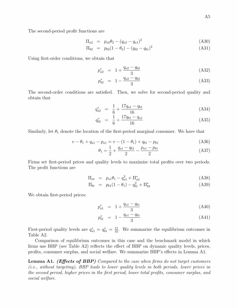
A5
The second-period profit functions are
Πa2 = pa2θ2 − (qa2 − qa1)2 (A30)
Πb2 = pb2(1− θ2)− (qb2 − qb1)2 (A31)
Using first-order conditions, we obtain that
p∗a2 = 1 +qa2 − qb2
3(A32)
p∗b2 = 1− qa2 − qb23
(A33)
The second-order conditions are satisfied. Then, we solve for second-period quality andobtain that
q∗a2 =1
6+
17qa1 − qb116
(A34)
q∗b2 =1
6+
17qb1 − qa116
(A35)
Similarly, let θ1 denote the location of the first-period marginal consumer. We have that
v − θ1 + qa1 − pa1 = v − (1− θ1) + qb1 − pb1 (A36)
θ1 =1
2+
qa1 − qb12
− pa1 − pb12
(A37)
Firms set first-period prices and quality levels to maximize total profits over two periods.The profit functions are
Πat = pa1θ1 − q2a1 +Π∗a2 (A38)
Πbt = pb1(1− θ1)− q2b1 +Π∗b2 (A39)
We obtain first-period prices:
p∗a1 = 1 +qa1 − qb1
3(A40)
p∗b1 = 1− qa1 − qb13
(A41)
First-period quality levels are q∗a1 = q∗b1 = 1132. We summarize the equilibrium outcomes in
Table A2.Comparison of equilibrium outcomes in this case and the benchmark model in which
firms use BBP (see Table A2) reflects the effect of BBP on dynamic quality levels, prices,profits, consumer surplus, and social welfare. We summarize BBP’s effects in Lemma A1.
Lemma A1. (Effects of BBP) Compared to the case when firms do not target customers(i.e., without targeting), BBP leads to lower quality levels in both periods, lower prices inthe second period, higher prices in the first period, lower total profits, consumer surplus, andsocial welfare.
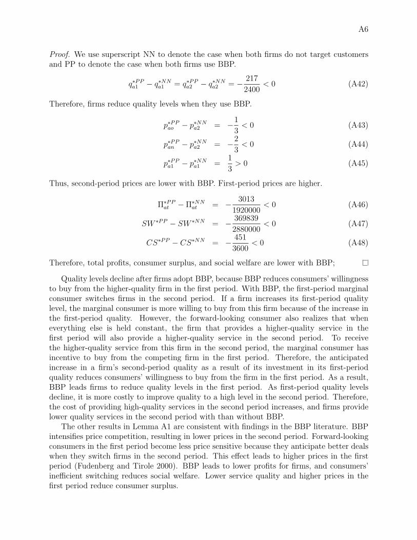
A6
Proof. We use superscript NN to denote the case when both firms do not target customersand PP to denote the case when both firms use BBP.
q∗PPa1 − q∗NN
a1 = q∗PPa2 − q∗NN
a2 = − 217
2400< 0 (A42)
Therefore, firms reduce quality levels when they use BBP.
p∗PPao − p∗NN
a2 = −1
3< 0 (A43)
p∗PPan − p∗NN
a2 = −2
3< 0 (A44)
p∗PPa1 − p∗NN
a1 =1
3> 0 (A45)
Thus, second-period prices are lower with BBP. First-period prices are higher.
Π∗PPat − Π∗NN
at = − 3013
1920000< 0 (A46)
SW ∗PP − SW ∗NN = − 369839
2880000< 0 (A47)
CS∗PP − CS∗NN = − 451
3600< 0 (A48)
Therefore, total profits, consumer surplus, and social welfare are lower with BBP;
Quality levels decline after firms adopt BBP, because BBP reduces consumers’ willingnessto buy from the higher-quality firm in the first period. With BBP, the first-period marginalconsumer switches firms in the second period. If a firm increases its first-period qualitylevel, the marginal consumer is more willing to buy from this firm because of the increase inthe first-period quality. However, the forward-looking consumer also realizes that wheneverything else is held constant, the firm that provides a higher-quality service in thefirst period will also provide a higher-quality service in the second period. To receivethe higher-quality service from this firm in the second period, the marginal consumer hasincentive to buy from the competing firm in the first period. Therefore, the anticipatedincrease in a firm’s second-period quality as a result of its investment in its first-periodquality reduces consumers’ willingness to buy from the firm in the first period. As a result,BBP leads firms to reduce quality levels in the first period. As first-period quality levelsdecline, it is more costly to improve quality to a high level in the second period. Therefore,the cost of providing high-quality services in the second period increases, and firms providelower quality services in the second period with than without BBP.
The other results in Lemma A1 are consistent with findings in the BBP literature. BBPintensifies price competition, resulting in lower prices in the second period. Forward-lookingconsumers in the first period become less price sensitive because they anticipate better dealswhen they switch firms in the second period. This effect leads to higher prices in the firstperiod (Fudenberg and Tirole 2000). BBP leads to lower profits for firms, and consumers’inefficient switching reduces social welfare. Lower service quality and higher prices in thefirst period reduce consumer surplus.

A7
A2 Second-Period Quality Reinitializes to Zero
Suppose that quality reinitializes to zero so that the cost of providing quality qi2 in period 2is a quadratic function of qi2 rather than the quality improvement qi2 − qi1. We can modifythe cost function in the models accordingly. Specifically, firms’ profit functions when theydo not customize quality are:
Πa2 = paoθa + pan(θb − θ1)− q2a2, (A49)
Πb2 = pbo(1− θb) + pbn(θ1 − θa)− q2b2. (A50)
Second-period prices are p∗an = 1− 4θ13
+ qa2−qb23
, p∗ao =1+2θ1
3+ qa2−qb2
3, p∗bn = 4θ1−1
3− qa2−qb2
3,
and p∗bo = 1− 2θ13− qa2−qb2
3. Second-period quality levels are q∗a2 =
521
− θ17and q∗b2 =
221
+ θ17.
The marginal consumer at θ1 faces the same trade-off as in the main model. We have
v − θ1 + qa1 − pa1 + [v − (1− θ1) + qe∗b2 − pe∗bn] = v − (1− θ1) + qb1 − pb1 + [v − θ1 + qe∗a2 − pe∗an] .
(A51)
With the second-period equilibrium quality and prices, we obtain
θ1 =1
2− 7(pa1 − pb1)
18+
7(qa1 − qb1)
18. (A52)
Firms’ profit functions at the beginning of the first period are
Πat = pa1θ1 +Π∗a2 − q2a1, (A53)
Πbt = pb1(1− θ1) + Π∗b2 − q2b1. (A54)
First-period prices are p∗a1 = 43+ 2(qa1−qb1)
25and p∗b1 = 4
3− 2(qa1−qb1)
25. We obtain first-period
quality levels q∗a1 = q∗b1 = 0.23. The rest of the equilibrium outcomes are summarized inTable 2.
When firms customize quality, their second-period profit functions are
Πa2 = paoθa + pan(θb − θ1)− γ(q2ao + q2an
), (A55)
Πb2 = pbo(1− θb) + pbn(θ1 − θa)− γ(q2bo + q2bn
). (A56)
Second-period prices are p∗an = 1− 4θ13
+ qan−qbo3
, p∗ao =1+2θ1
3+ qao−qbn
3, p∗bn = 4θ1−1
3− qao−qbn
3,
and p∗bo = 1 − 2θ13
− qan−qbo3
. Second-period quality levels are q∗ao = 4θ121
+ 17, q∗an = 1
3− 10θ1
21,
q∗bo =13− 4θ1
21, q∗bn = 10θ1
21− 1
7.
We solve for first-period marginal consumer as before:
v − θ1 + qa1 − pa1 + [v − (1− θ1) + qe∗bn − pe∗bn] = v − (1− θ1) + qb1 − pb1 + [v − θ1 + qe∗an − pe∗an] ,
θ1 =1
2− 21(pa1 − pb1)
40+
21(qa1 − qb1)
40. (A57)

A8
Firms’ profit functions at the beginning of the first period are
Πat = pa1θ1 +Π∗a2 − q2a1, (A58)
Πbt = pb1(1− θ1) + Π∗b2 − q2b1. (A59)
First-period prices are p∗a1 =2021+ 11(qa1−qb1)
83and p∗b1 =
2021− 11(qa1−qb1)
83. We obtain first-period
quality levels q∗a1 = q∗b1 =47166
≈ 0.283. The rest of the equilibrium outcomes are summarizedin Table 2 of the paper. Comparison of equilibrium outcomes show that all propositions inthe main model continue to hold.
A3 A Marginal Cost of Quality Provision
We generalize the cost functions to allow for a marginal cost of quality provision. Wesolve the benchmark model without quality discrimination and the main model with qualitydiscrimination separately below.
A3.1 Benchmark Model: Without Quality Discrimination
The marginal consumers are located at the same places as before. We have
v − θa + qa2 − pao = v − (1− θa) + qb2 − pbn, (A60)
θa =1
2+
qa2 − qb22
− pao − pbn2
. (A61)
v − θb + qa2 − pan = v − (1− θb) + qb2 − pbo, (A62)
θb =1
2+
qa2 − qb22
− pan − pbo2
. (A63)
Firms’ profit functions in the second period are
Πa2 = (pao − κqa2)θa + (pan − κqa2)(θb − θ1)− q2a2, (A64)
Πb2 = (pbo − κqb2)(1− θb) + (pbn − κqb2)(θ1 − θa)− q2b2. (A65)
We obtain second-period prices:
p∗an = 1− 4θ13
+qa2 − qb2 + κ(qb2 + 2qa2)
3(A66)
p∗ao =1
3+
2θ13
+qa2 − qb2 + κ(2qa2 + qb2)
3(A67)
p∗bn =4θ13
− 1
3+
qb2 − qa2 + κ(qa2 + 2qb2)
3(A68)
p∗bo = 1− 2θ13
+qb2 − qa2 + κ(qa2 + 2qb2)
3(A69)

A9
The second-period quality levels are
q∗a2 =κ(κ2 − 3κ− 3) + 3θ1(κ− 1) + 5
3(7 + 4κ− 2κ2)(A70)
q∗b2 =κ2(κ− 3) + 3θ1(1− κ) + 2
3(7 + 4κ− 2κ2)(A71)
The first-period marginal consumer is located at θ1. We have that
v − θ1 − pa1 + [v − (1− θ1) + qe∗b2 − pe∗bn] = v − (1− θ1)− pb1 + (v − θ1 + qe∗a2 − pe∗an) (A72)
θ1 =9 + 7(pb1 − pa1) + 2κ2(pa1 − pb1)− 3κ2 + 4κ(pb1 − pa1) + 6κ
6(3 + 2κ− κ2)(A73)
The total profits that firms maximize in the first period are
Πat = pa1θ1 +Π∗a2, (A74)
Πbt = pb1(1− θ1) + Π∗b2. (A75)
We obtain first-period prices that p∗a1 = p∗b1 = 43. Table A1 summarizes the equilibrium
outcomes.
A3.2 Main Model: With Quality Discrimination
When firms offer different quality levels to repeat and new customers in the second period,the second-period marginal consumers are located at
v − θa + qao − pao = v − (1− θa) + qbn − pbn, (A76)
θa =1
2+
qao − qbn2
− pao − pbn2
. (A77)
v − θb + qan − pan = v − (1− θb) + qbo − pbo, (A78)
θb =1
2+
qan − qbo2
− pan − pbo2
. (A79)
With the general cost function, firms’ profit functions in the second period are
Πa2 = (pao − κqao)θa + (pan − κqan)(θb − θ1)− γ(q2ao + q2an
), (A80)
Πb2 = (pbo − κqbo)(1− θb) + (pbn − κqbn)(θ1 − θa)− γ(q2bo + q2bn
). (A81)
We obtain the second-period equilibrium prices:
p∗an = 1− 4θ13
+qan − qbo + κ(qbo + 2qan)
3(A82)
p∗ao =1
3+
2θ13
+qao − qbn + κ(2qao + qbn)
3(A83)

A10
p∗bn =4θ13
− 1
3+
qbn − qao + κ(qao + 2qbn)
3(A84)
p∗bo = 1− 2θ13
+qbo − qan + κ(qan + 2qbo)
3(A85)
Then, we solve for second-period quality levels
q∗an =(1− κ)(1− θ1 − 9γ − κ2θ1 + κ2 + 2κθ1 + 12γθ1 − 2κ)
6γ(κ2 − 2κ− 9γ + 1)(A86)
q∗ao =(1− κ)(θ1 − 3γ + κ2θ1 − 2κθ1 − 6γθ1)
6γ(κ2 − 2κ− 9γ + 1)(A87)
q∗bn =(1− κ)(θ1 + 3γ + κ2θ1 − 2κθ1 − 12γθ1)
6γ(κ2 − 2κ− 9γ + 1)(A88)
q∗bo =(1− κ)(1− θ1 − 9γ − 2κ+ 6γθ1 − κ2θ1 + κ2 + 2κθ1)
6γ(κ2 − 2κ− 9γ + 1)(A89)
The first-period marginal consumers are located at θ1. We have that
v − θ1 − pa1 + [v − (1− θ1) + qe∗bn − pe∗bn] = v − (1− θ1)− pb1 + [v − θ1 + qe∗an − pe∗an] (A90)
θ1 =1
2+
3γ(pa1 − pb1)(κ2 − 2κ− 9γ + 1)
(κ2 − 2κ− 12γ + 1)(κ2 − 2κ− 6γ + 1)(A91)
Firms set first-period prices to maximize total profits over two periods. The profit functionsare
Πat = pa1θ1 +Π∗a2, (A92)
Πbt = pb1(1− θ1) + Π∗b2. (A93)
We obtain first-period prices:
p∗a1 = p∗b1 =(1− 6γ + κ2 − 2κ)(12γ − 1− κ2 + 2κ)
6γ(1− 9γ + κ2 − 2κ)(A94)
Table A1 summarizes the equilibrium outcomes.
A3.3 Verification of Main Results
We focus on the region of κ and γ in which the profit functions are concave in quality andprices. We verify that main results in the paper continue to hold.
q∗ao − q∗an =1− κ
2(9γ − 1 + 2κ− κ2)> 0 (A95)
p∗ao − p∗an =6γ + κ− κ2
2(9γ − 1 + 2κ− κ2)> 0 (A96)
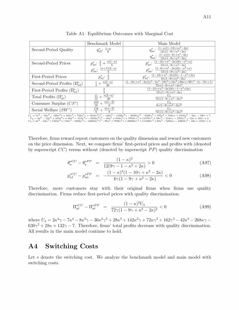
A11
Table A1: Equilibrium Outcomes with Marginal Cost
Benchmark Model Main Model
Second-Period Quality q∗a2:1−κ6
q∗ao:(1−κ)(1−12γ+κ2−2κ)12γ(1−9γ+κ2−2κ)
q∗an:(1−κ)(1−6γ+κ2−2κ)12γ(1−9γ+κ2−2κ)
Second-Period Prices p∗ao:23+ κ(1−κ)
6p∗ao:
(1−12γ+κ2−2κ)(6γ−κ2+κ)12γ(1−9γ+κ2−2κ)
p∗an:(κ+1)(2−κ)
6p∗an:
(1−6γ+κ2−2κ)(6γ−κ2+κ)12γ(1−9γ+κ2−2κ)
First-Period Prices p∗a1:43
p∗a1:(1−12γ+κ2−2κ)(6γ−1−κ2+2κ)
6γ(1−9γ+κ2−2κ)
Second-Period Profits (Π∗a2)
14+ κ(2−κ)
36(1−18γ+κ2−2κ)(κ4−4κ3−18κ2γ+6κ2+36κγ+90γ2−4γ−18γ+1)
72γ(1−9γ+κ2−2κ)2
First-Period Profits (Π∗a1)
23
(1−12γ+κ2−2κ)(6γ−1−κ2+2κ)12γ(1−9γ+κ2−2κ)
Total Profits (Π∗at)
1112
+ κ(2−κ)36
U1
72γ(1−9γ+κ2−2κ)2
Consumer Surplus (CS∗) 31918
+ κ(κ−2)6
U2
8γ(1−9γ+κ2−2κ)2
Social Welfare (SW ∗) 1769
+ κ(κ−2)9
U3
72γ(1−9γ+κ2−2κ)2
U1 = 7κ6 − 42κ5 − 198κ4γ + 105κ4 + 792κ3γ + 1818κ2γ2 − 140κ3 − 1188κ2γ − 3636κγ2 − 5508γ3 + 105κ2 + 792κγ + 1818γ2 − 42κ − 198γ + 7.U2 = 2κ6 − 12κ5 + 103κ4γ + 30κ4 − 412κ3γ − 2352κ2γ2 − 40κ3 + 618κ2γ + 4704κγ2 + 11376γ3 + 30κ2 − 412κγ − 2352γ2 − 12κ + 103γ + 2.
U3 = 4κ6 −24κ5 +1323κ4γ+60κ4 −5292κ3γ−24804κ2γ2 −80κ3 +7938κ2γ+49608κγ2 +113400γ3 +60κ2 −5292κγ−24804γ2 −24κ+1323γ+4.
Therefore, firms reward repeat customers on the quality dimension and reward new customerson the price dimension. Next, we compare firms’ first-period prices and profits with (denotedby superscript CC) versus without (denoted by superscript PP ) quality discrimination
θ∗CCa − θ∗PP
a =(1− κ)2
12(9γ − 1− κ2 + 2κ)> 0 (A97)
p∗CCa1 − p∗PP
an = −(1− κ)2(1− 10γ + κ2 − 2κ)
6γ(1− 9γ + κ2 − 2κ)< 0 (A98)
Therefore, more customers stay with their original firms when firms use qualitydiscrimination. Firms reduce first-period prices with quality discrimination.
Π∗CCat − Π∗PP
at =(1− κ)2U4
72γ(1− 9γ + κ2 − 2κ)2< 0 (A99)
where U4 = 2κ4γ − 7κ4 − 8κ3γ − 36κ2γ2 +28κ3 +142κ2γ +72κγ2 +162γ3 − 42κ2 − 268κγ −630γ2 + 28κ+ 132γ − 7. Therefore, firms’ total profits decrease with quality discrimination.All results in the main model continue to hold.
A4 Switching Costs
Let s denote the switching cost. We analyze the benchmark model and main model withswitching costs.

A12
A4.1 Benchmark Model
When firms use BBP and consumers incur switching costs, the marginal consumers in thesecond period become:
v − θa + qa2 − pao = v − (1− θa) + qb2 − pbn − s, (A100)
θa =1 + s
2+
qa2 − qb22
− pao − pbn2
. (A101)
v − θb + qa2 − pan − s = v − (1− θb) + qb2 − pbo, (A102)
θb =1− s
2+
qa2 − qb22
− pan − pbo2
. (A103)
Firms maximize second-period profit functions:
Πa2 = paoθa + pan(θb − θ1)− (qa2 − qa1)2, (A104)
Πb2 = pbo(1− θb) + pbn(θ1 − θa)− (qb2 − qb1)2. (A105)
Second-period prices are p∗an = 3−4θ1−s3
+ qa2−qb23
, p∗ao =1+s+2θ1
3+ qa2−qb2
3, p∗bn = 4θ1−1−s
3+ qb2−qa2
3,
and p∗bo = 3−2θ1+s3
+ qb2−qa23
. Second-period quality levels are q∗a2 = 521
− θ17+ 8qa1−qb1
7and
q∗b2 =221
+ θ17+ 8qb1−qa1
7. The first-period marginal consumer is located at θ1. We have
v − θ1 + qa1 − pa1 + [v − (1− θ1) + qe∗b2 − pe∗bn − s] = v − (1− θ1) + qb1 − pb1 + [v − θ1 + qe∗a2 − pe∗an − s]
θ1 =1
2+
2(qa1 − qb1)
9+
7(pb1 − pa1)
18. (A106)
The total profits that firms maximize in the first period are
Πat = pa1θ1 +Π∗a2 − q2a1, (A107)
Πbt = pb1(1− θ1) + Π∗b2 − q2b1. (A108)
We solve for the first-period equilibrium prices and obtain p∗a1 = 43+ 8(qa1−qb1)
25− 2s
3and
p∗b1 = 43+ 8(qb1−qa1)
25− 2s
3. The first-period equilibrium quality levels are q∗a1 = q∗b1 = 19
75. We
summarize the rest of the equilibrium outcomes in Table 3 of the paper.
A4.2 Main Model
When both firms customize quality and consumers incur switching costs, the second-periodmarginal consumers are
v − θa + qao − pao = v − (1− θa) + qbn − pbn − s, (A109)
θa =1 + s
2+
qao − qbn2
− pao − pbn2
. (A110)
v − θb + qan − pan − s = v − (1− θb) + qbo − pbo, (A111)
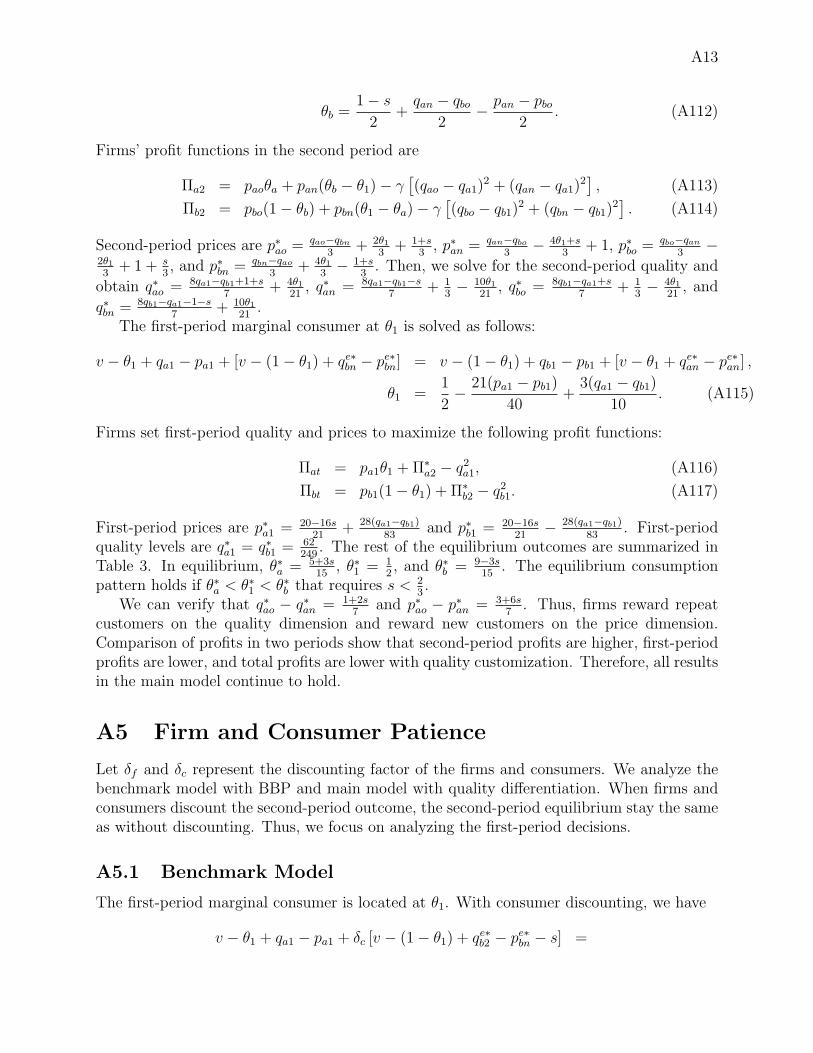
A13
θb =1− s
2+
qan − qbo2
− pan − pbo2
. (A112)
Firms’ profit functions in the second period are
Πa2 = paoθa + pan(θb − θ1)− γ[(qao − qa1)
2 + (qan − qa1)2], (A113)
Πb2 = pbo(1− θb) + pbn(θ1 − θa)− γ[(qbo − qb1)
2 + (qbn − qb1)2]. (A114)
Second-period prices are p∗ao =qao−qbn
3+ 2θ1
3+ 1+s
3, p∗an = qan−qbo
3− 4θ1+s
3+ 1, p∗bo =
qbo−qan3
−2θ13
+ 1 + s3, and p∗bn = qbn−qao
3+ 4θ1
3− 1+s
3. Then, we solve for the second-period quality and
obtain q∗ao = 8qa1−qb1+1+s7
+ 4θ121, q∗an = 8qa1−qb1−s
7+ 1
3− 10θ1
21, q∗bo = 8qb1−qa1+s
7+ 1
3− 4θ1
21, and
q∗bn = 8qb1−qa1−1−s7
+ 10θ121
.The first-period marginal consumer at θ1 is solved as follows:
v − θ1 + qa1 − pa1 + [v − (1− θ1) + qe∗bn − pe∗bn] = v − (1− θ1) + qb1 − pb1 + [v − θ1 + qe∗an − pe∗an] ,
θ1 =1
2− 21(pa1 − pb1)
40+
3(qa1 − qb1)
10. (A115)
Firms set first-period quality and prices to maximize the following profit functions:
Πat = pa1θ1 +Π∗a2 − q2a1, (A116)
Πbt = pb1(1− θ1) + Π∗b2 − q2b1. (A117)
First-period prices are p∗a1 = 20−16s21
+ 28(qa1−qb1)83
and p∗b1 = 20−16s21
− 28(qa1−qb1)83
. First-periodquality levels are q∗a1 = q∗b1 = 62
249. The rest of the equilibrium outcomes are summarized in
Table 3. In equilibrium, θ∗a = 5+3s15
, θ∗1 = 12, and θ∗b = 9−3s
15. The equilibrium consumption
pattern holds if θ∗a < θ∗1 < θ∗b that requires s < 23.
We can verify that q∗ao − q∗an = 1+2s7
and p∗ao − p∗an = 3+6s7
. Thus, firms reward repeatcustomers on the quality dimension and reward new customers on the price dimension.Comparison of profits in two periods show that second-period profits are higher, first-periodprofits are lower, and total profits are lower with quality customization. Therefore, all resultsin the main model continue to hold.
A5 Firm and Consumer Patience
Let δf and δc represent the discounting factor of the firms and consumers. We analyze thebenchmark model with BBP and main model with quality differentiation. When firms andconsumers discount the second-period outcome, the second-period equilibrium stay the sameas without discounting. Thus, we focus on analyzing the first-period decisions.
A5.1 Benchmark Model
The first-period marginal consumer is located at θ1. With consumer discounting, we have
v − θ1 + qa1 − pa1 + δc [v − (1− θ1) + qe∗b2 − pe∗bn − s] =

A14
v − (1− θ1) + qb1 − pb1 + δc [v − θ1 + qe∗a2 − pe∗an − s]
θ1 =1
2− 3δc(qa1 − qb1) + 7(pa1 − pb1 + qb1 − qa1)
7 + 2δc(A118)
The total profits that firms maximize in the first period are
Πat = pa1θ1 +Π∗a2 − q2a1, (A119)
Πbt = pb1(1− θ1) + Π∗b2 − q2b1. (A120)
We solve for the first-period equilibrium prices and quality and obtain q∗a1 = q∗b1 =686+273δf−98δc−608δ2f+363δcδf−84δ2c
84(49+14δc−38δf ). In equilibrium, the first-period price is p∗a1 = p∗b1 =
2δc7+
δf21+1.
A5.2 Main Model
Again, the second-period analysis is the same as in the main model because firm andconsumer discounting does not affect the second-period decisions. The first-period marginalconsumer at θ1 is solved as follows:
v − θ1 + qa1 − pa1 + δc [v − (1− θ1) + qe∗bn − pe∗bn] = v − (1− θ1) + qb1 − pb1 + δc [v − θ1 + qe∗an − pe∗an] ,
θ1 =1
2− 3 [3δc(qa1 − qb1) + 7(pa1 − pb1 + qb1 − qa1)]
21− δc(A121)
Firms set first-period quality and prices to maximize the following profit functions:
Πat = pa1θ1 +Π∗a2 − q2a1, (A122)
Πbt = pb1(1− θ1) + Π∗b2 − q2b1. (A123)
First-period equilibrium quality levels are q∗a1 = q∗b1 =9261+189δ2c+1656δcδf−7424δ2f−4410δc+4200δf
42(1323−63δc−928δf ).
Equilibrium first-period prices are p∗a1 = p∗b1 = 1− δc21.
A5.3 Verification of Main Results
With firm and consumer patience, proposition 1 remains the same as the second-periodoutcomes do not change. To see this, q∗CC
ao − q∗CCan = 1
7, p∗CC
ao − p∗CCan = 3
7, and
Π∗CCa2 − Π∗PP
a2 = 231764
. Proposition 2 holds as p∗CCa1 − p∗PP
a1 = − δc3
− δf21
< 0 andΠ∗CC
at − Π∗PPat = U1
7056(63δc+928δf−1323)2(14δc−38δf+49)2< 0, where U1 = 244268136δ5cδf +
2382098985δ4cδ2f − 11529899136δ3cδ
3f + 3807147008δ2cδ
4f + 39685259264δcδ
5f − 914838624δ5c −
27535138596δ4cδf − 46187599332δ3cδ2f + 905390869712δ2cδ
3f − 1541574429696δcδ
4f −
106895622144δ5f + 31947782832δ4c + 191482856208δ3cδf − 3752254963786δ2cδ2f +
7858122606432δcδ3f + 440868841472δ4f − 143183135592δ3c + 5156406567900δ2cδf −
15993413416036δcδ2f − 452079659696δ3f − 2364819724764δ2c + 14728301634816δcδf −
350037350551δ2f−5126298229584δc+853188665616δf−386633673468 < 0. CS∗CC−CS∗PP =U2
1764(63δc+928δf−1323)(14δc−38δf+49)> 0, where U2 = 484659δ3cδf + 738528δ2cδ
2f + 532728δ3c +
5677805δ2cδf − 19901192δcδ2f − 2962176δ3f − 9322740δ2c + 55604857δcδf + 7812168δ2f −

A15
39155508δc − 5092521δf . SW ∗CC − SW ∗PP = U3
3528(63δc+928δf−1323)2(14δc−38δf+49)2> 0,
where U3 = 1099206612δ5cδf + 13957694541δ4cδ2f − 30058089600δ3cδ
3f − 48279755776δ2cδ
4f +
39685259264δcδ5f +24893568δ5c − 21189211218δ4cδf +71491174244δ3cδ
2f +219317898352δ2cδ
3f −
200769442816δcδ4f +102020726784δ5f −871274880δ4c −42413713020δ3cδf −291898325418δ2cδ
2f +
313767351072δcδ3f −562934177792δ4f +3964300704δ3c +65020703076δ2cδf −65943090444δcδ
2f +
1165856105456δ3f+64038703680δ2c−220188103632δcδf−1074067015931δ2f+134481277728δc+371380010022δf > 0 for δc, δf ∈ [0, 1].
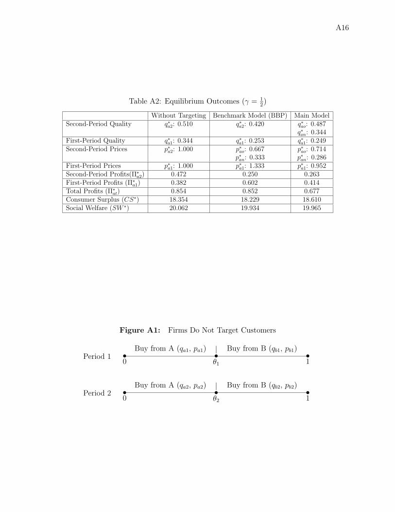
A16
Table A2: Equilibrium Outcomes (γ = 12)
Without Targeting Benchmark Model (BBP) Main ModelSecond-Period Quality q∗a2: 0.510 q∗a2: 0.420 q∗ao: 0.487
q∗an: 0.344First-Period Quality q∗a1: 0.344 q∗a1: 0.253 q∗a1: 0.249Second-Period Prices p∗a2: 1.000 p∗ao: 0.667 p∗ao: 0.714
p∗an: 0.333 p∗an: 0.286First-Period Prices p∗a1: 1.000 p∗a1: 1.333 p∗a1: 0.952Second-Period Profits(Π∗
a2) 0.472 0.250 0.263First-Period Profits (Π∗
a1) 0.382 0.602 0.414Total Profits (Π∗
at) 0.854 0.852 0.677Consumer Surplus (CS∗) 18.354 18.229 18.610Social Welfare (SW ∗) 20.062 19.934 19.965
Figure A1: Firms Do Not Target Customers
•0
•θ1
|Buy from A (qa1, pa1) Buy from B (qb1, pb1)•1
Period 1
•0
•θ2
|Buy from A (qa2, pa2) Buy from B (qb2, pb2)•1
Period 2