BEFORE THE MINNESOTA OFFICE OF ADMINISTRATIVE HEARINGS … · BEFORE THE MINNESOTA OFFICE OF...

$: BEFORE THE MINNESOTA OFFICE OF ADMINISTRATIVE HEARINGS … · BEFORE THE MINNESOTA OFFICE OF ADMINISTRATIVE HEARINGS 600 North Robert Street St. Paul, MN 55101 ... R.Dessler\rhttps:$
PUC Docket No. E-999/CI-14-643

OAH Docket No. 80-2500-31888

Clean Energy Organizations

Exhibit ________

BEFORE THE MINNESOTA OFFICE OF ADMINISTRATIVE HEARINGS

600 North Robert Street

St. Paul, MN 55101

FOR THE MINNESOTA PUBLIC UTILITIES COMMISSION

121 Seventh Place East, Suite 350

St Paul, MN 55101-2147

In the Matter of the Further

Investigation into Environmental and

Socioeconomic Costs Under

Minnesota Statute 216B.2422, Subd. 3


OAH Docket No. 80-2500-31888

REBUTTAL TESTIMONY OF DR. ANDREW DESSLER,

Professor in the Department of Atmospheric Sciences

Texas A&M University

On Behalf of


John Mashey

Text Box

R.Dessler https://www.edockets.state.mn.us/EFiling/edockets/searchDocuments.do?method=showPoup&documentId={C36B70CA-5848-4A60-A1D0-1664F0E5250C}&documentTitle=20158-113193-04 REBUTS: Happer, Lindzen, Spencer SURREBUTALS BY: Happer, Lindzen, Spencer p.4 Focus on ECS claims by the above. p.5 "One of the guiding principles of science is to use all of the available data when testing hypotheses. Reliable science does not throw out the vast majority of the data that disagrees with a hypothesis, and then use the remaining tiny fraction to conclude that the sought-after result is correct. This type of "cherry picking" is how Drs. Spencer, Lindzen, and Happer reach the conclusions in their testimony. " p.6 "Specifically, it is incorrect to say that: ECS is "extremely unlikely to exceed 2°C." (Dr. Lindzen) "The temperature increase for doubling CO2 levels appears to be close to the feedback-free doubling sensitivity of S = 1 K." (Dr. Happer) " p.7 "In addition, Drs. Spencer, Lindzen, and Happer only discuss estimates of ECS 9 based on the 20th century record. This is another example of cherry picking --10 other analyses of ECS, such as those from paleoclimate data and from model 11 simulations, suggest ECS values nearer to the top of the IPCC range. " p.8 "I do not view the satellite record as a robust data set, and I would not trust it to 10 guide climate policy." (reviews history of errors and corrections), see also R.Abraham. p.14 "Thus, I view the satellite record as a work in progress, and it is far from the "gold standard" that Drs. Spencer, Lindzen, and Happer present it as. And I do not judge the satellite record to be of sufficient quality to use it to (in)validate the climate models." p.15 "It is also worth noting that skeptics frequently make claims about the surface record that, upon cursory examination, turn out to be wrong. ... Dr. Lindzen stood before the House of Commons and accused a major NASA center of fraud based on a plot that he clearly knew nothing about." (He had gotten a plot from someone else and had not checked it.) p.22 "Thus, I find that Drs. Spencer, Lindzen, and Happer's claim that climate change has stopped, or paused, is incorrect. " pp.34-42 CV


OAH Docket No. 80-2500-31888


Exhibit ________

i

TABLE OF CONTENTS

I. EXPERT EXPERIENCE ............................................................................................. 1

II. OVERVIEW OF TESTIMONY .................................................................................. 2

III. SPECIFIC RESPONSES OR CORRECTIONS ......................................................... 4

A. Equilibrium Climate Sensitivity ........................................................................... 4

B. Temperature Data ................................................................................................. 8

C. No Evidence of a Warming “Hiatus” ................................................................. 15

D. Accuracy of Models ........................................................................................... 23

E. Extreme Weather ................................................................................................ 26

IV. CONCLUSION ......................................................................................................... 28

V. REFERENCES ............................................................................................................. i


OAH Docket No. 80-2500-31888


Exhibit ________

1

I. EXPERT EXPERIENCE 1

Q. Please state your name and address for the record. 2

A. My name is Andrew Dessler. My address is 5110 Congressional Dr., College 3

Station, Texas 77845. 4

Q. What is your educational background and profession? 5

A. I am currently a professor in the Department of Atmospheric Sciences at Texas 6

A&M University. I have a Bachelor of Arts degree in physics from Rice 7

University, a Doctor of Philosophy (“Ph.D.”) in chemistry from Harvard 8

University, and I spent two years doing postdoctoral research at NASA in 9

Greenbelt, Maryland. Prior to taking my job at Texas A&M University in 2005, I 10

was on the research faculty in the Department of Meteorology and the Earth 11

System Science Interdisciplinary Center at the University of Maryland. My 12

complete curriculum vitae is attached as Schedule 1 to this testimony. 13

Q. Please describe the work you have done related to global warming, if any. 14

A. My research for the past decade has focused on water vapor and clouds, both of 15

which play an important role in regulating our climate. On the policy side, I spent 16

a year as a Senior Policy Analyst in the White House Office of Science and 17

Technology Policy, where I was the Office’s staff atmospheric scientist. Based on 18

my experience, I have co-authored two books on climate change: “The Science 19

and Politics of Global Climate Change: A Guide to the Debate” (Cambridge 20


OAH Docket No. 80-2500-31888


Exhibit ________

2

University Press, 2006, 2010); and “Introduction to Modern Climate Change” 1

(Cambridge University Press, 2012, 2015). 2

Q. Does your current profession require you to keep informed of developments 3

and to maintain your in-depth understanding of global warming issues? 4

A. Yes. 5

II. OVERVIEW OF TESTIMONY 6

Q. What is the purpose of your testimony? 7

A. I have been asked by the Minnesota Center for Environmental Advocacy, Fresh 8

Energy, Sierra Club, and the Izaak Walton League of America – Midwest Office 9

(collectively “Clean Energy Organizations”) to respond to opinions and assertions 10

offered in the direct testimony submitted on behalf of Peabody Energy by Dr. 11

William Happer, Dr. Roy Spencer, and Dr. Richard Lindzen criticizing the 12

equilibrium climate sensitivity assumption used by the Interagency Working 13

Group (“IWG”) to develop a Social Cost of Carbon. 14

Q. Please explain what “equilibrium climate sensitivity” is. 15

A. Equilibrium climate sensitivity (hereafter “ECS”) is typically defined to be the 16

warming in response to a doubling of atmospheric carbon dioxide from pre-17

industrial amounts (280 parts per million) to twice that (560 parts per million), 18

after equilibrium is established. The Intergovernmental Panel on Climate Change 19

(“IPCC”) reviewed all of the evidence in the peer-reviewed literature and 20


OAH Docket No. 80-2500-31888


Exhibit ________

3

concluded in their 2007 Fourth Assessment Report that the likely range for the 1

ECS was 2-4.5°C. The IWG used this estimate, along with an economic model, to 2

estimate the cost of the damage caused by a ton of carbon dioxide released to the 3

atmosphere. In the IPCC’s 2013 Fifth Assessment Report, the likely range was 4

slightly expanded to 1.5-4.5°C. 5

Q. Have you reviewed the direct testimony submitted in this proceeding by Dr. 6

Roy Spencer, Dr. Richard Lindzen, and Dr. William Happer? 7

A. Yes. 8

Q. What is your overall impression of their testimony? 9

A. I find that the conclusions offered in their testimony are unreliable because they 10

have not employed unbiased and rigorous scientific methods. One of the guiding 11

principles of science is to use all of the available data when testing hypotheses. 12

Reliable science does not throw out the vast majority of the data that disagrees 13

with a hypothesis, and then use the remaining tiny fraction to conclude that the 14

sought-after result is correct. This type of “cherry picking” is how Drs. Spencer, 15

Lindzen, and Happer reach the conclusions in their testimony. Looking at all of 16

the data strongly supports the fundamental conclusions that the Earth is warming, 17

humans are extremely likely responsible for the recent warming, and future 18

warming carries with it the risk of significant harm—the exact opposite of what 19

they concluded. In my testimony, I will point out many of the places where Drs. 20

John Mashey

Highlight

John Mashey

Highlight


OAH Docket No. 80-2500-31888


Exhibit ________

4

Spencer, Lindzen, and Happer relied on cherry picking to support otherwise 1

untenable scientific positions. 2

III. SPECIFIC RESPONSES OR CORRECTIONS 3

Q. Do you have responses or corrections to specific assertions in the testimony of 4

Drs. Spencer, Lindzen, and Happer? 5

A. Yes. In this testimony I will first give my opinion regarding the general assertion 6

by Drs. Spencer, Lindzen, and Happer that the ECS assumed by the IWG is too 7

large. Next, I will discuss the primary bases for this general assertion, namely that 8

the satellite temperature data show a “hiatus” in the warming trend of global 9

average temperatures and that models significantly overestimate the warming that 10

will occur in the coming decades. Lastly, I provide a response to the assertion that 11

there has been no increase in extreme weather due to climate change. 12

A. Equilibrium Climate Sensitivity 13

Q. Drs. Spencer, Lindzen, and Happer all claim that the ECS is below the 14

IPCC’s canonical range of 1.5-4.5°C for doubled carbon dioxide. Do you 15

agree? 16

A. No. Specifically, it is incorrect to say that: 17

ECS is “extremely unlikely to exceed 2°C.” (Dr. Lindzen) 18

“The temperature increase for doubling CO2 levels appears to be close to the 19

feedback-free doubling sensitivity of S = 1 K.” (Dr. Happer) 20


OAH Docket No. 80-2500-31888


Exhibit ________

5

In fact, none of the credible peer-reviewed literature cited supports either of those 1

claims. 2

It is true that several recent estimates have uncertainty ranges that extend to low 3

values. Thus, Dr. Spencer’s testimony is most accurate when he says that ECS is 4

“possibly as low as 1°C or less.” What he neglects to say, however, is that these 5

same analyses also allow much higher values of ECS—well within the IPCC’s 6

ECS range. Thus, while these measurements allow a low ECS value, they also 7

allow higher values in the upper end of the IPCC’s range. 8

In addition, Drs. Spencer, Lindzen, and Happer only discuss estimates of ECS 9

based on the 20th

century record. This is another example of cherry picking—10

other analyses of ECS, such as those from paleoclimate data and from model 11

simulations, suggest ECS values nearer to the top of the IPCC range. 12

Thus, while there is some evidence that ECS is near the bottom of the IPCC 13

range, there is other evidence that it is nearer to the top. That is why the IPCC 14

range is as wide as it is. 15

Q. Drs. Spencer, Lindzen, and Happer all suggest that a small amount of 16

warming due to increased carbon dioxide emissions might be beneficial for 17

the Earth. Is warming of a few degrees significant? 18

A. A few degrees may not seem like much warming to some. After all, summer days 19

can be 50°C warmer than the winter days and daytime can be 25°C warmer than 20

the following night. And one day can be several tens of degrees Celsius warmer 21

John Mashey

Highlight

John Mashey

Highlight


OAH Docket No. 80-2500-31888


Exhibit ________

6

or cooler than the next. If you consider these ranges of temperature variations, 1

changes in the global average of a few degrees Celsius may sound insignificant. 2

In this case, however, this common intuition is wrong. Although the temperature 3

in any single place can vary considerably by season, by day, and even by hour, the 4

variations tend to cancel when averaged over the entire globe. When you are 5

experiencing the warmth of daytime, someone on the other side of the globe is 6

experiencing the coolness of night. When it is summer where you live, it is winter 7

in the other hemisphere. Heat waves in one location are generally canceled by a 8

cold spell somewhere else. In other words, the large temperature variations you 9

experience are nearly completely canceled by opposite variations somewhere else 10

on the Earth. 11

Because of this cancellation, the global average temperature of the Earth is very 12

stable, with year-to-year temperature variations of just a few tenths of a degree. 13

Moreover, seemingly small changes in global average temperature are associated 14

with significant shifts in the Earth’s climate. For example, the global annual 15

average temperature during the last ice age was about 10°F colder than that of our 16

present climate. At that time, the Earth was basically a different planet: glaciers 17

covered much of North America and Europe, leading to a very different 18

distribution of ecosystems, and because so much water was tied up in glaciers, sea 19

level was approximately 400 feet lower than it is today. 20

John Mashey

Highlight

John Mashey

Highlight


OAH Docket No. 80-2500-31888


Exhibit ________

7

During the summer of 2003, a heat wave struck Europe in which the average 1

temperature in Europe was about 3°C above average. Despite this seemingly 2

small amount of warming, this heat wave caused the deaths of several tens of 3

thousands of people. And temperatures a few hundred years ago were about 1°C 4

cooler than today—a large enough difference that we refer to that period as the 5

Little Ice Age. 6

Furthermore, it is not just the magnitude of the warming but also the rate of 7

warming that is of concern. It took more than 10,000 years for the planet to warm 8

5°C and emerge from the last ice age—an average rate of 0.05°C per century. The 9

rate of warming predicted for the twenty-first century is a few degrees per 10

century—about 100 times faster. Rate matters because the faster the warming 11

occurs, the less time people and natural ecosystems have to adapt to the changes. 12

If the sea level rises one meter in 1,000 years, we could likely adapt to that change 13

without too much trouble. But a one-meter increase in sea level in a century 14

would be much more expensive to adjust to. And a one-meter increase in a decade 15

would be a disaster, displacing millions of people and destroying trillions of 16

dollars of infrastructure. 17

John Mashey

Highlight

John Mashey

Highlight


OAH Docket No. 80-2500-31888


Exhibit ________

8

B. Temperature Data 1

Q. Much of Drs. Spencer, Lindzen, and Happer’s testimony claiming that the 2

ECS assumed by the IWG is too high is based on measurements of the 3

Earth’s temperature. What temperature records are available? 4

A. There are several widely used records, including the surface thermometer and 5

satellite records. Weather balloon records are also discussed, but are much less 6

frequently used by the scientific community for reasons discussed below. 7

Q. Drs. Spencer, Lindzen, and Happer all emphasize the satellite record, 8

particularly Dr. Spencer. What is your opinion of that data set? 9

A. I do not view the satellite record as a robust data set, and I would not trust it to 10

guide climate policy. A review of its history provides justification for my views. 11

Dr. Spencer and his colleague John Christy first published this data set in 1990. 12

Surprisingly, Spencer and Christy’s data showed a cooling trend (Christy et al., 13

19951) in the mid-1990s. This result was surprising given that all of the other data 14

at that time showed the climate system was warming. 15

In 1998, Wentz and Schabel discovered that Spencer and Christy had neglected 16

the decay of the satellites’ orbit in their trend calculation. Spencer and Christy 17

acknowledged this problem and updated their algorithm to incorporate this effect 18

(Christy et al., 2000). Despite their correction, there was no significant change to 19

the cooling trend they saw. This was at least partially because, when correcting 20

1 A complete list of references cited in this testimony appears at the end.

John Mashey

Highlight

John Mashey

Highlight

John Mashey

Highlight

John Mashey

Highlight

John Mashey

Highlight


OAH Docket No. 80-2500-31888


Exhibit ________

9

for their last error, they introduced a new error into their algorithm—an incorrect 1

diurnal cycle.2 2

In 2004, Fu et al. discovered that the tropospheric temperature trend in the 3

satellite record was contaminated by stratospheric cooling. That is, the trend 4

measured by the satellite was a combination of warming of the troposphere and 5

cooling of the stratosphere. They offset each other to some extent, causing the 6

resulting trend to be lower than the actual tropospheric trend. This was not, 7

strictly speaking, an error. However, it underlines the complexity of the satellite 8

temperature measurement and the fact that, even 15 years after the data set was 9

first published, the scientific community was still learning what the measurements 10

actually meant. 11

In 2005, Mears and Wentz discovered the diurnal cycle problem that Spencer and 12

Christy introduced when they corrected for the orbit decay problem. To 13

understand how the diurnal cycle affects the trend, imagine that a satellite flies 14

over a location at 2 PM each day and takes a measurement of that location’s 15

temperature. Over time, the satellite’s orbit drifts so that it flies over that location 16

later and later each day. After a few years, the satellite is flying over that location 17

at 3 PM. Because temperatures rise throughout the day, it is generally warmer at 18

that location at 3 PM than it is at 2 PM. Thus, the drift in the satellite’s orbit 19

2 The diurnal cycle refers to the daily cycle of temperatures: warming during the day and

cooling at night.

John Mashey

Highlight

John Mashey

Highlight

John Mashey

Highlight

John Mashey

Highlight


OAH Docket No. 80-2500-31888


Exhibit ________

10

would by itself introduce a warming trend, even if the climate were not actually 1

changing. This artifact must also be identified and adjusted for. 2

Here’s what Mears and Wentz said in a letter to Science in response to a letter 3

from Spencer and Christy in 2005: 4

Once we realized that the diurnal correction being used by Christy and 5

Spencer for the lower troposphere had the opposite sign from their 6

correction for the middle troposphere sign, we knew that something was 7

amiss. Clearly, the lower troposphere does not warm at night and cool in 8

the middle of the day. We question why Christy and Spencer adopted an 9

obviously wrong diurnal correction in the first place. They first 10

implemented it in 1998 in response to Wentz and Schabel [1998], which 11

found a previous error in their methodology: neglecting the effects of orbit 12

decay. 13

In the years since, new problems with the satellite temperature record keep being 14

identified. Po-Chedley and Fu, 2012, pointed out issues with how Spencer and 15

Christy constructed their satellite time series. This problem arises because the 16

record is stitched together from data gathered by about a dozen satellites, each of 17

which lasts just a few years before it fails and is replaced by the next. This makes 18

the temperature trend highly sensitive to how the records from successive 19

satellites are intercalibrated. To understand this, suppose you are trying to watch 20

your weight, but your scale breaks and a month passes before you buy a new one. 21

If the new scale says you are two pounds heavier than your last reading on the old 22

one, does this mean you have gained two pounds? Or does the new scale just read 23

two pounds heavier than the old one? You could tell which of these was the case 24

if you bought a new scale before the old one broke, and measured yourself on 25

John Mashey

Highlight

John Mashey

Highlight

John Mashey

Highlight


OAH Docket No. 80-2500-31888


Exhibit ________

11

both scales for a while to estimate the difference between them—if you had the 1

foresight, patience, and money to do this. 2

The U.S. Government has tried to do this by launching each new satellite while 3

the previous one is still operating. That way, overlapping measurements can be 4

collected long enough to calibrate the new instrument. But since it is impossible 5

to predict exactly when an instrument is going to fail, they have not been entirely 6

successful in obtaining records that overlap for a sufficient period of time. As a 7

result, the temperature trend estimated from the satellite data is quite sensitive to 8

how one connects data between these satellites. After analyzing the methodology, 9

Po-Chedley and Fu, 2012, concluded that the way Spencer and Christy stitched 10

the satellites together artificially reduced the global mid-tropospheric trend by 11

0.042°C per decade for 1979–2009. 12

Most recently, Po-Chedley et al., 2015, have revisited the issue of diurnal cycle 13

corrections and found that problems still remain in the trend calculations from 14

these satellites. 15

Q. What are your conclusions about using satellite temperature data based on 16

this history? 17

A. From this history, I extract three important points. First, every few years, 18

significant new issues are discovered in the satellite temperature record, some of 19

which are still being resolved. Second, the errors Spencer and Christy make 20

always tend to reduce the trend—i.e., they work to lessen the magnitude of 21

John Mashey

Highlight

John Mashey

Highlight


OAH Docket No. 80-2500-31888


Exhibit ________

12

climate change. Third, Spencer and Christy never discover these issues 1

themselves. 2

Thus, I view the satellite record as a work in progress, and it is far from the “gold 3

standard” that Drs. Spencer, Lindzen, and Happer present it as. And I do not judge 4

the satellite record to be of sufficient quality to use it to (in)validate the climate 5

models. 6

Q. Are balloon radiosonde data more reliable? 7

A. No. In my opinion, the radiosonde, or weather balloon, record is another 8

unreliable data set. Issues with data homogenization (e.g., shifts in the trend due 9

to changes in instrumentation) are even bigger problems than they are for the 10

satellite record. 11

Also, as with the satellite record, scientists are continually uncovering issues with 12

the data set. Sherwood et al., 2005, for example, found an uncorrected bias in the 13

trend caused by daytime solar heating of the balloon instrument. And the 14

methodology used to calculate the trends can have a huge impact on the answer 15

one gets. In a recent paper, Sherwood and Nishant, 2015, used a novel 16

homogenization technique to calculate an atmospheric warming in good 17

agreement with the climate models. 18

One might view the supposed agreement between the satellite and balloon records 19

as validations of both data sets. However, such comparisons have not identified 20

the many problems in the satellite data, described above. Thus, the satellite-21

John Mashey

Highlight

John Mashey

Highlight

John Mashey

Highlight

John Mashey

Highlight


OAH Docket No. 80-2500-31888


Exhibit ________

13

balloon temperature comparisons appear to be a very loose check on either data 1

set. Overall, like the satellite data, I do not judge the balloon record to be of 2

sufficient quality to use it to (in)validate the climate models. 3

Q. Drs. Spencer, Lindzen, and Happer claim that the surface record has biases 4

in it. What’s your opinion of that claim? 5

A. In the mid-2000s, criticisms about the poor quality of the surface thermometer 6

network surfaced. Some thermometers were admittedly placed in locations (e.g., a 7

parking lot) that could cause reasonable people to wonder whether there was 8

contamination in the long-term surface thermometer temperature record. 9

But the scientists who produce and maintain these records have been aware of this 10

issue for decades and account for changes in station location, as well as many 11

other factors, when calculating the temperature trends. After claims were made 12

about poor siting, this issue was reexamined by independent groups (e.g., 13

Hausfather et al., 2013; Wickham et al., 2013). In all cases, the surface 14

temperature record has emerged unscathed. 15

It is also worth noting that skeptics frequently make claims about the surface 16

record that, upon cursory examination, turn out to be wrong. For example, in 17

2012, during testimony to the UK House of Commons, Lindzen claimed to have 18

found evidence that NASA Goddard Institute for Space Studies (“GISS”) was 19

John Mashey

Highlight

John Mashey

Highlight

John Mashey

Highlight


OAH Docket No. 80-2500-31888


Exhibit ________

14

nefariously manipulating data3 to inflate the warming trend. It turned out that his 1

“evidence” was actually a simple mistake on his part, and no evidence of data 2

tampering exists.4 3

When the error was pointed out, Lindzen issued a correction5 that acknowledged 4

that he took the plot from someone else and that he had done no work to verify 5

the contents of the plot. This episode is deeply revealing about climate skeptics in 6

general and Dr. Lindzen in particular. Dr. Lindzen stood before the House of 7

Commons and accused a major NASA center of fraud based on a plot that he 8

clearly knew nothing about. The fact that Dr. Lindzen throws accusations of fraud 9

around so freely, without even a cursory checking of the facts, speaks volumes 10

about the quality of his skepticism. I can assure you that his testimony in this case 11

shows the same level of scholarship and due diligence as his claim of tampering 12

in the NASA GISS data. 13

Q. So what do you view as the most reliable data set? 14

A. My view is that the surface thermometer record is the most reliable data set. To 15

reach this conclusion, one need only compare the history of the surface 16

thermometer record with that of the satellite record. As discussed above, every 17

few years another major problem in the satellite record is discovered, and there is 18

3 http://i.telegraph.co.uk/multimedia/archive/02148/RSL-

HouseOfCommons_2148505a.pdf, slide 12. 4 http://www.realclimate.org/index.php/archives/2012/03/misrepresentation-from-

lindzen/. 5 https://web.archive.org/web/20140720170731/http://repealtheact.org.uk/blog/apology-

from-prof-lindzen-for-howard-haydens-nasa-giss-data-interpretation-error.

John Mashey

Highlight

John Mashey

Highlight


OAH Docket No. 80-2500-31888


Exhibit ________

15

abundant evidence of on-going issues in the data set (e.g., the diurnal cycle 1

correction). The surface thermometer record, on the other hand, because of its 2

central role in the climate debate, has undergone incredible scrutiny over the last 3

decade and has emerged unscathed. In the end, there is absolutely no legitimate 4

scientific reason to reject the surface record in favor of the satellite record, and 5

there are many good reasons to consider the surface record superior to the satellite 6

record. 7

C. No Evidence of a Warming “Hiatus” 8

Q. Has the climate stopped changing over the past two decades? 9

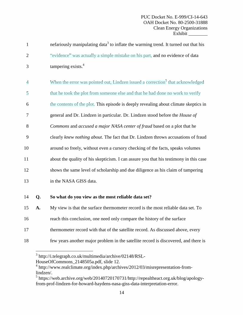
A. No, the climate is still changing. Figure 1 shows the trend in surface air 10

temperature between the date on the x-axis and March 2015 (the most recent 11

available month). The trend is positive for every month, except January 2005, 12

thereby demonstrating that the climate has been (nearly) continuously warming 13

since the late 1970s. 14

John Mashey

Highlight

John Mashey

Highlight


OAH Docket No. 80-2500-31888


Exhibit ________

16

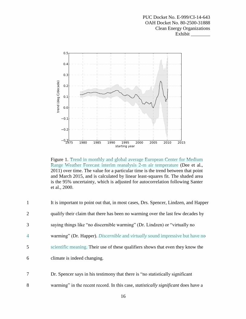
Figure 1. Trend in monthly and global average European Center for Medium

Range Weather Forecast interim reanalysis 2-m air temperature (Dee et al.,

2011) over time. The value for a particular time is the trend between that point

and March 2015, and is calculated by linear least-squares fit. The shaded area

is the 95% uncertainty, which is adjusted for autocorrelation following Santer

et al., 2000.

It is important to point out that, in most cases, Drs. Spencer, Lindzen, and Happer 1

qualify their claim that there has been no warming over the last few decades by 2

saying things like “no discernible warming” (Dr. Lindzen) or “virtually no 3

warming” (Dr. Happer). Discernible and virtually sound impressive but have no 4

scientific meaning. Their use of these qualifiers shows that even they know the 5

climate is indeed changing. 6

Dr. Spencer says in his testimony that there is “no statistically significant 7

warming” in the recent record. In this case, statistically significant does have a 8

John Mashey

Highlight

John Mashey

Highlight


OAH Docket No. 80-2500-31888


Exhibit ________

17

specific scientific meaning. It means that the error bars on the trend extend below 1

zero—so you cannot exclude a trend of zero. This is quite different from saying 2

that there is no trend, and Dr. Spencer is capitalizing on the fact that most people 3

do not understand the nuances of the language of statistics. 4

Figure 1 shows that Dr. Spencer is correct: beginning around 2000, the 5

uncertainty in the trend expands and begins to encompass zero. Thus, it is correct 6

to say that there has been no statistically significant warming since 2000. But this 7

does not mean the trend is zero, close to zero, or even small. It means that the 8

trend is smaller than the uncertainty. It seems quite clear to me that Drs. Spencer, 9

Lindzen, and Happer recognize this, which is why they have to qualify their 10

claims. 11

In addition, Drs. Spencer, Lindzen, and Happer only investigate a single metric 12

for climate change: global average temperature. This is not necessarily an 13

unreasonable choice, but there are many other metrics one should look at before 14

claiming that climate change had stopped. This is yet another example of cherry 15

picking in their testimony. 16

John Mashey

Highlight

John Mashey

Highlight


OAH Docket No. 80-2500-31888


Exhibit ________

18

If one looks at the spatial distribution of temperature change rather than global 1

average temperature for example, quite a different picture of trends over the last 2

two decades emerges. Figure 2 shows that most of the globe has warmed 3

considerably since the 1980s and 1990s, except for the Eastern Pacific, which has 4

actually cooled. The cooling in the Eastern Pacific largely offsets the warming in 5

the rest of the planet, leading to the reduced global average trends apparent since 6

the early 2000s, shown in Figure 1. Thus, our climate is changing, even though 7

the global average temperature may not be changing much. 8

Figure 2. Mean annual surface temperature differences from NASA GISS

Surface Temperature Analysis for 1999–2012 and 1976–1998 in °C, with

zonal means at right for ocean (blue), land (red), and zonal mean (black).

From Trenberth and Fasullo, 2013.

John Mashey

Highlight


OAH Docket No. 80-2500-31888


Exhibit ________

19

Other measures of climate change may very well be better predictors of the 1

impact that increased concentrations of greenhouse gases will have on our planet. 2

Indeed, as discussed by Dr. John Abraham in his Rebuttal Testimony, most of the 3

energy trapped by greenhouse gases goes into the ocean, so that changes in ocean 4

heat content (“OHC”) are an important indicator of climate change. Figure 3 5

shows OHC has increased rapidly since 1998, even as the rate of warming of the 6

surface temperature has slowed. 7

Figure 3. Ocean heat content (“OHC”) integrated from 0 to 300 m (grey), 700

m (blue), and total depth (violet) from a reanalysis system, as represented by

its 5 ensemble members. The time series show monthly anomalies smoothed

with a 12 month running mean, with respect to the 1958-1965 base period.

Hatching extends over the range of the ensemble members and hence the

spread gives a measure of the uncertainty. The vertical colored bars indicate a

2 year interval following volcanic eruptions with a 6 month lead (owing to the

12 month running mean), and the 1997-1998 El Nino event again with 6

months on either side. On lower right, the linear slope for a set of global

heating rates (W/m2) is given. After Fig. 1 of Balmaseda et al., 2013.

John Mashey

Highlight

John Mashey

Highlight


OAH Docket No. 80-2500-31888


Exhibit ________

20

Finally, Figure 4 shows a time series of the 95th

percentile temperatures over land; 1

this figure demonstrates that the warmest 5 percent of observed temperatures have 2

risen rapidly over the period that Drs. Spencer, Lindzen, and Happer claim that 3

climate change has stopped. In other words, extreme temperatures over land are 4

becoming more extreme. This result is consistent with Figure 2, which shows that 5

land areas have continued warming over the past decade. 6

Figure 4. The time series are the ERA-Interim 95th percentile of the maximum

temperature over land (Txp95_Land, red) and the global (ocean + land) mean

temperature (Tm_Glob) in ERA-Interim (blue) and HadCRUT4 (black). The

anomalies are computed with respect to the 1979-2010 time period. From Fig. 2

of Seneviratne et al., 2014.

Thus, I find that Drs. Spencer, Lindzen, and Happer’s claim that climate change 7

has stopped, or paused, is incorrect. A more complete and less biased examination 8

John Mashey

Highlight


OAH Docket No. 80-2500-31888


Exhibit ________

21

of the data yields the exact opposite conclusion to the one advanced by Drs. 1

Spencer, Lindzen, and Happer—that, indeed, climate change continues unabated. 2

Q. Has the rate of warming slowed down over the last decade or so? 3

A. Yes. Figure 1 shows that the warming since the beginning of the 21st century has 4

been smaller than that since the 1990s (although the differences are not 5

statistically significant). 6

Q. Does a smaller trend over a decade or so tell you anything about the long-7

term trajectory of the climate? 8

A. No. The trend over short periods (e.g., a decade) can deviate significantly from 9

the long-term trend. As an example, Figure 5 shows a time series of monthly and 10

global average surface temperature from the surface thermometer record. Also 11

shown as short black segments are trends based on endpoints that were carefully 12

selected to produce cooling trends. As you can see, it is possible to generate a 13

continuous set of short-term cooling trends, even as the climate is experiencing a 14

long-term warming. All you have to do is start the trend calculation during a 15

particularly hot year (e.g., an El Niño year) and then end it in a cool year (e.g., a 16

La Niña or volcanic year). 17

John Mashey

Highlight


OAH Docket No. 80-2500-31888


Exhibit ________

22

Figure 5. A plot of monthly and global average surface temperature from the

surface thermometer record (gray line) along with short-term trend lines (black

lines). Data are from the NASA GISS Surface Temperature Analysis (Hansen et

al., 2010), downloaded from data.giss.nasa.gov/gistemp/. This was taken from

Fig. 2.5 of Dessler, Introduction to Modern Climate Change, 2nd

edition, to be

published in Sept. 2015 by Cambridge Univ. Press.


OAH Docket No. 80-2500-31888


Exhibit ________

23

The existence of these short-term negative trends allows people like Drs. Spencer, 1

Lindzen, and Happer to claim during almost any year covered by Figure 5 that 2

global warming had stopped or even that the Earth had entered a cooling period. 3

But in reality, the short-term cooling trends provide zero information about the 4

long-term trajectory and it is not accurate for Drs. Spencer, Lindzen, and Happer 5

to imply otherwise. 6

D. Accuracy of Models 7

Q. Drs. Spencer, Lindzen, and Happer all claim that climate models have 8

overpredicted temperature increases when compared to observations. In 9

your opinion, have models been able to simulate the 20th

century historical 10

record? 11

A. Yes. Figure 6 shows a comparison between climate models and observations, and 12

the overall agreement between models and observations is excellent. In particular, 13

I see no evidence supporting Dr. Spencer’s claim that climate models have 14

warmed two to three times faster than the observations over the last thrity-five to 15

fifty-five years. 16

John Mashey

Highlight


OAH Docket No. 80-2500-31888


Exhibit ________

24

Figure 6. Three observational estimates of global mean surface temperature

(black lines) from the Hadley Centre/Climatic Research Unit gridded surface

temperature data set (HadCRUT4), Goddard Institute for Space Studies

Surface Temperature Analysis (GISTEMP), and Merged Land-Ocean Surface

Temperature Analysis (MLOST), compared to model simulations (CMIP3

models – thin blue lines and CMIP5 models – thin yellow lines) with

anthropogenic and natural forcings. After Figure TS.9 of the Technical

Summary of the 2013 IPCC Working Group I report.

Q. Have models been able to simulate temperature changes during the last one 1

to two decades? 2

A. For long-term comparisons, such as that in Figure 6, short-term fluctuations (e.g., 3

El Nino cycles and volcanic eruptions) have little effect on the comparison. But 4

when comparing periods of a decade or two, they can have a huge effect. As 5

demonstrated in Figure 5, sometimes these short-term variations can produce a 6

short-term negative trend during a period long-term warming. 7

John Mashey

Highlight

John Mashey

Highlight

John Mashey

Highlight


OAH Docket No. 80-2500-31888


Exhibit ________

25

So the key to comparing short-term trends in models and observations is to 1

account for these short-term variations in the comparison. This means that 2

comparing the observed temperature time series to an average of an ensemble of 3

models, as done in the testimony of Drs. Spencer, Lindzen, and Happer (see, e.g., 4

Figures 1 and 3 of Dr. Spencer’s Exhibit 2), will not produce accurate results. In 5

an ensemble of models, the highs and lows caused by the short-term variability do 6

not occur at the same time. When many model runs are averaged together, the 7

short-term ups and downs cancel out and you get a smooth increase in 8

temperature. When such an ensemble average is compared to a single time series, 9

full of ups and downs, the agreement may look terrible. This is certainly a major 10

problem with Drs. Spencer, Lindzen, and Happer’s comparisons. 11

To do this comparison correctly, the models must incorproate the same the exact 12

phasing of short-term variability as is in the observations. Recent publications 13

have actually done this and it substantially improves the comparison between the 14

models and observations (Dai et al., 2015; Huber and Knutti, 2014). 15

Another issue with the model-data comparison is that the models assumed 16

incorrect “forcing”6 over the last decade. In particular, the models assumed a 17

brighter sun than we actually had, which causes the models to run “hot.” And the 18

models do not include the effects of several small volcanic eruptions that occurred 19

6 “Forcing” is an imposed energy imbalance imposed on the planetary system. Addition

of CO2 causes a forcing, as do changes in the intensity of the Sun, addition of aerosols,

etc. In response to a forcing, the planet’s temperature adjusts until it reestablishes energy

balance.

John Mashey

Highlight

John Mashey

Highlight

John Mashey

Highlight


OAH Docket No. 80-2500-31888


Exhibit ________

26

in the last decade. This also tends to make the models run “hot.” Accounting for 1

these errors in the forcings of the models improves agreement between the models 2

and observations (Huber and Knutti, 2014). 3

In the end, the models do a reasonable job of simulating the last decade, just as 4

they do a reasonable job of simulating the last century. I therefore find no 5

evidence that climate models have been programmed to be too sensitive, as 6

suggested by these witnesses. 7

E. Extreme Weather 8

Q. Drs. Spencer, Lindzen, and Happer also claim that there is no evidence that 9

extreme weather events are increasing in frequency or intensity due to 10

climate change. Do you agree? 11

A. No. These statements are false. For example, Dr. Happer writes: 12

There is not the slightest evidence for any increase in extreme weather 13

events, as summarized by the Senate Testimony of 1 August, 2012 by 14

John Christy, which I reference in my prepared report. 15

But Figure 4 clearly shows an increase in extreme heat events. And by relying on 16

the testimony of John Christy, Dr. Happer is also relying on a source that is 17

several years old, not published in the peer-reviewed literature, and widely 18

disputed by the scientific community. 19

In fact, a wide array of peer-reviewed analyses have indicated that humans are 20

playing an increasingly important role in extreme temperature and precipitation 21

John Mashey

Highlight


OAH Docket No. 80-2500-31888


Exhibit ________

27

events (Christidis et al., 2011; Fischer and Knutti, 2015; Min et al., 2011; Min et 1

al., 2013; Morak et al., 2013). And rising sea level is making extreme sea level 2

events more damaging, even when the weather event driving the sea level is not 3

more extreme. For example, the increase in sea level over the 20th

century made 4

the storm surge from Hurricane Sandy more damaging and more costly than it 5

would otherwise have been.7 And given the strong connection between 6

temperature and sea level, we can expect sea level to continue to rise due to 7

human activities—and bring with it more intense extreme sea level events. 8

Finally, while not exactly an “extreme event,” the ongoing acidification of the 9

ocean due to the release of carbon dioxide could have dire consequences (Orr et 10

al., 2005). Two billion people on the planet rely on protein from the ocean, and 11

changes in ocean ecosystems due to changing ocean chemistry could severely 12

stress those food supplies. 13

7 https://www.climate.gov/news-features/features/superstorm-sandy-and-sea-level-rise.

John Mashey

Highlight


OAH Docket No. 80-2500-31888


Exhibit ________

28

IV. CONCLUSION 1

Q. What are the most important aspects of climate change you would like the 2

Public Utilities Commission to know? 3

A. 4

1. The climate has changed over the last century, and the climate has continued to 5

change over the last decade or so. 6

2. There is no evidence that our predictions of several degrees Celsius of warming 7

over the next 100 years are wrong. 8

3. A few degrees Celsius in global average warming is a huge amount of warming 9

for human society and ecosystems. 10

Q. Does this conclude your testimony? 11

A. Yes. 12


OAH Docket No. 80-2500-31888


Exhibit ________

i

V. REFERENCES

Balmaseda, M. A., K. E. Trenberth, and E. Kaellen (2013), Distinctive climate signals in

reanalysis of global ocean heat content, Geophys. Res. Lett., 40, 1754-1759, doi:

10.1002/grl.50382.

Christidis, N., P. A. Stott, and S. J. Brown (2011), The Role of Human Activity in the

Recent Warming of Extremely Warm Daytime Temperatures, J. Climate, 24, 1922-1930,

doi: 10.1175/2011JCLI4150.1.

Christy, J. R., R. W. Spencer, and R. T. McNider (1995), Reducing noise in the MSU

daily lower-tropospheric global temperature dataset, J. Climate, 8, 888-896, doi:

10.1175/1520-0442(1995)008<0888:rnitmd>2.0.co;2.

Christy, J. R., R. W. Spencer, and W. D. Braswell (2000), MSU tropospheric

temperatures: Dataset construction and radiosonde comparisons, Journal of Atmospheric

and Oceanic Technology, 17, 1153-1170, doi: 10.1175/1520-

0426(2000)017<1153:mttdca>2.0.co;2.

Dai, A., J. C. Fyfe, S.-P. Xie, and X. Dai (2015), Decadal modulation of global surface

temperature by internal climate variability, Nature Clim. Change, 5, 555-559, doi:

10.1038/nclimate2605

http://www.nature.com/nclimate/journal/v5/n6/abs/nclimate2605.html - supplementary-

information.

Fischer, E. M., and R. Knutti (2015), Anthropogenic contribution to global occurrence of

heavy-precipitation and high-temperature extremes, Nature Clim. Change, 5, 560-564,

doi: 10.1038/nclimate2617


information.

Fu, Q., C. M. Johanson, S. G. Warren, and D. J. Seidel (2004), Contribution of

stratospheric cooling to satellite-inferred tropospheric temperature trends, Nature, 429,

55-58, doi: 10.1038/nature02524.

Hansen, J., R. Ruedy, M. Sato, and K. Lo (2010), Global surface temperature change,

Rev. Geophys., 48, Rg4004, doi: 10.1029/2010rg000345.

Hausfather, Z., M. J. Menne, C. N. Williams, T. Masters, R. Broberg, and D. Jones

(2013), Quantifying the effect of urbanization on U.S. Historical Climatology Network

temperature records, Journal of Geophysical Research: Atmospheres, 118, 481-494, doi:

10.1029/2012JD018509.

http://www.nature.com/nclimate/journal/v5/n6/abs/nclimate2605.html#supplementary-information





OAH Docket No. 80-2500-31888


Exhibit ________

ii

Huber, M., and R. Knutti (2014), Natural variability, radiative forcing and climate

response in the recent hiatus reconciled, Nature Geosci, 7, 651-656, doi:

10.1038/ngeo2228

http://www.nature.com/ngeo/journal/v7/n9/abs/ngeo2228.html - supplementary-

information.

Mears, C. A., and F. J. Wentz (2005), The effect of diurnal correction on satellite-derived

lower tropospheric temperature, Science, 309, 1548-1551, doi: 10.1126/science.1114772.

Min, S.-K., X. Zhang, F. W. Zwiers, and G. C. Hegerl (2011), Human contribution to

more-intense precipitation extremes, Nature, 470, 378-381, doi:

http://www.nature.com/nature/journal/v470/n7334/abs/10.1038-nature09763-

unlocked.html - supplementary-information.

Min, S.-K., X. Zhang, F. Zwiers, H. Shiogama, Y.-S. Tung, and M. Wehner (2013),

Multimodel detection and attribution of extreme temperature changes, J. Climate, 26,

7430-7451, doi: 10.1175/JCLI-D-12-00551.1.

Morak, S., G. C. Hegerl, and N. Christidis (2013), Detectable Changes in the Frequency

of Temperature Extremes, J. Climate, 26, 1561-1574, doi: 10.1175/JCLI-D-11-00678.1.

Orr, J. C., et al. (2005), Anthropogenic ocean acidification over the twenty-first century

and its impact on calcifying organisms, Nature, 437, 681-686, doi:

http://www.nature.com/nature/journal/v437/n7059/suppinfo/nature04095_S1.html.

Po-Chedley, S., and Q. Fu (2012), A Bias in the Midtropospheric Channel Warm Target

Factor on the NOAA-9 Microwave Sounding Unit, Journal of Atmospheric and Oceanic

Technology, 29, 646-652, doi: 10.1175/jtech-d-11-00147.1.

Po-Chedley, S., T. J. Thorsen, and Q. Fu (2015), Removing Diurnal Cycle Contamination

in Satellite-Derived Tropospheric Temperatures: Understanding Tropical Tropospheric

Trend Discrepancies, J. Climate, 28, 2274-2290, doi: 10.1175/jcli-d-13-00767.1.

Seneviratne, S. I., M. G. Donat, B. Mueller, and L. V. Alexander (2014), No pause in the

increase of hot temperature extremes, Nature Clim. Change, 4, 161-163, doi:

10.1038/nclimate2145


information.

Sherwood, S. C., J. R. Lanzante, and C. L. Meyer (2005), Radiosonde Daytime Biases

and Late-20th Century Warming, Science, 309, 1556-1559, doi:

10.1126/science.1115640.

http://www.nature.com/ngeo/journal/v7/n9/abs/ngeo2228.html#supplementary-information

http://www.nature.com/ngeo/journal/v7/n9/abs/ngeo2228.html#supplementary-information

http://www.nature.com/nature/journal/v470/n7334/abs/10.1038-nature09763-unlocked.html#supplementary-information

http://www.nature.com/nature/journal/v470/n7334/abs/10.1038-nature09763-unlocked.html#supplementary-information

http://www.nature.com/nature/journal/v437/n7059/suppinfo/nature04095_S1.html




OAH Docket No. 80-2500-31888


Exhibit ________

iii

Sherwood, S. C., and N. Nishant (2015), Atmospheric changes through 2012 as shown by

iteratively homogenized radiosonde temperature and wind data (IUKv2), Environmental

Research Letters, 10, 7, doi: 10.1088/1748-9326/10/5/054007.

Wentz, F. J., and M. Schabel (1998), Effects of orbital decay on satellite-derived lower-

tropospheric temperature trends, Nature, 394, 661-664, doi: 10.1038/29267.

Wickham, C., R. Rohde, R. A. Muller, J. Wurtele, J. Curry, D. Groom, R. Jacobsen, S.

Perlmutter, A. Rosenfeld, and S. Mosher (2013), Influence of urban heating on the global

temperature land average using rural sites identified from MODIS classifications,

Geoinfo. Geostat., 1:2, doi: 10.4172/gigs.1000104.

PUC Docket No. E-999/CI-14-643 Dr. Andrew Dessler Rebuttal Testimony

OAH Docket No. 80-2500-31888 Clean Energy Organizations

Schedule 1

Exhibit ___

Schedule 1, Page 1

Andrew E. Dessler

Address

Dept. of Atmospheric Sciences

Texas A&M University

TAMU 3150

College Station, TX 77845

Telephone: 979-862-1427

Fax: 979-862-4466 E-mail: [email protected]

Research Areas: Climate change, climate feedbacks, remote sensing, climate

change policy

Education: 1994 - Ph.D. - Chemistry, Harvard University

1990 - A.M. - Chemistry, Harvard University

1986 - B.A. - Physics, Rice University

Employment 2007-present Professor, Dept. of Atmospheric Sciences,

Texas A&M University 2005-2007 Associate Professor, Dept. of Atmospheric

Sciences, Texas A&M University 2000 Senior Policy Analyst, White House Office of

Science and Technology Policy, Environment

Division, Washington, DC 1998-2005 Associate Research Scientist, Earth System

Science Interdisciplinary Center (ESSIC), Univ.

of Maryland, College Park, MD 1996-1998 Assistant Research Scientist, ESSIC and the

Dept. of Meteorology 1994-1996 National Research Council Research

Associateship in the Atmospheric Chemistry

and Dynamics Branch of NASA Goddard Space

Flight Center, Greenbelt, MD.

Awards 2014 AMS Louis J. Battan Author’s Award for

Introduction to Modern Climate Change

2014 Texas A&M Association of Former Students

Teaching Award (College of Geosciences)

2012 AGU Atmospheric Sciences Ascent Award

2011 Google Science Communication Fellow

2011

Texas A&M College of Geosciences

Distinguished Achievement Award for Faculty

Research



Schedule 1

Exhibit ___

Schedule 1, Page 2

2011

Texas A&M Sigma Xi Outstanding

Communicator Award 2006 Aldo Leopold Leadership Program Fellowship

1999 NASA Goddard Laboratory for Atmospheres

Best Senior Author Publication Award for “A

reexamination of the ‘stratospheric fountain’

hypothesis” [Geophys. Res. Lett., 1998]. 1999 NASA New Investigator Award recipient

1994-1996 National Research Council Research

Associateship 1993 AGU Atmospheric Sciences Section

Outstanding Student Paper Award 1991-1994 NASA Graduate Student Fellowship in Global

Change Research

Notable recent invited presentations 2012 Woods Hole, H. Burr Steinbech at-large scholar

2012 NCAR ASP Thompson Lecturer

2012 Truman Distinguished Lecturer Series, Sandia National Laboratories

Leadership positions and notable committees 2012-2015

Chair of AAAS Section W (atmospheric and hydrospheric

sciences)

2013-2016 Member, AMS Climate and Radiation Committee

2014-2017 Member, NASA Earth Science Subcommittee

2011, 2015 NASA Earth Science Senior Review for Mission Extension

Teaching:

• GEOS 444: The science and politics of global climate change: A guide to the debate.

Developed this course, which is taught as part of the Enviromental Sciences

curriculum.

• GEOS 210: Climate change. Developed this course, which is taught as part of the

Enviromental Sciences curriculum.

• ATMO 602: Atmospheric physics (Fall 13 and 14)

• ATMO 685, Climate modeling (Fall 06)

• ATMO 201, Atmospheric Science (Fall 07)

Graduate students:

Hyun Cheol Kim – Ph.D. (Univ. of Maryland), 2005



Schedule 1

Exhibit ___

Schedule 1, Page 3

Joonsuk Lee – Ph.D, 2007, co-chair (with P. Yang)

Allison Cardona – M.A. 2008

Jeremy Solbrig – M.A. 2009

Sean Casey — Ph.D. 2009

A. Verma — M.A. 2011

Tao Wang — M.A. 2011

A. Christenberry — M.A. 2013

Tao Wang — Ph.D. 2014

Chen Zhou — Ph.D. 2014

chaired 2 masters recipients while at the Univ. of Maryland (1998 and 1999)

H. Ye — Ph.D., current

K. Smalley — M.A., current

S. Zhai — M.A., current

W. Yu — M.A., current

X. Wang — M.A., current

Postdoctoral Associates:

Christian Alcala (2001-2002), Sun Wong (2003-2005), Likun Wang (2004-2005), Wei

Wu (2005-2006)

Research Scientist:

Sun Wong (2005-2009)

Books A. E. Dessler, The chemistry and physics of stratospheric ozone, Academic Press, San

Diego, 2000.

A. E. Dessler and E. A. Parson, The science and politics of global climate change: A

guide to the debate, Cambridge Univ. Press, first edition 2006, second edition 2010, third

edition expected 2016.

A. E. Dessler, Introduction to modern climate change, Cambridge Univ. Press, first

edition 2011, second edition sent to publisher, publication expected 2015.

Refereed Publications

(‘*’ indicates a graduate student or postdoc first author)

*Wang, T., A.E. Dessler, M.R. Schoeberl, W.J. Randel, and J.-E. Kim, The impact of

temperature vertical structure on trajectory modeling of stratospheric water

vapor, Atmos. Chem. Phys., 15, 3517-3526, doi:10.5194/acp-15-3517-2015,

2015.



Schedule 1

Exhibit ___

Schedule 1, Page 4

*Zhou, C., A.E. Dessler, M.D. Zelinka, P. Yang, and T. Wang, Cirrus feedback on

interannual climate fluctuations, Geophys. Res. Lett., 41, 9166–9173,

doi:10.1002/2014GL062095, 2014.

Schoeberl M. R., A.E. Dessler, T. Wang, M.A. Avery, and E.J. Jensen, Cloud formation,

convection, and stratospheric dehydration, Earth and Space Science, 1,

doi:10.1002/2014EA000014, 2014.

Dessler, A.E., M.R. Schoeberl, T. Wang, S.M. Davis, K.H. Rosenlof, and J.-P. Vernier,

Variations of stratospheric water vapor over the past three decades, J. Geophys.

Res., 119, doi:10.1002/2014JD021712, 2014.

Dessler, A.E. and M.D. Zelinka, Climate Feedbacks. Encyclopedia of Atmospheric

Sciences, eds. G.R. North, J. Pyle, and F. Zhang, 2nd edition, Vol 2, pp. 18–25,

2014.

*Wang, T., W.J. Randel, A.E. Dessler, M.R. Schoeberl, and D.E. Kinnison, Trajectory

model simulations of ozone (O3) and carbon monoxide (CO) in the lower

stratosphere, Atmos. Chem. Phys., 14, 7135-7147, doi:10.5194/acp-14-7135-

2014, 2014.

*Wang, C., P. Yang, A.E. Dessler, B.A. Baum, and Y. Hu, Estimation of the cirrus cloud

scattering phase function from satellite observations, Journal of Quantitative

Spectroscopy and Radiative Transfer, 138, 36-49, doi:

10.1016/j.jqsrt.2014.02.001, 2014.

*Kummer, J.R. and A.E. Dessler, The impact of forcing efficacy on the equilibrium

climate sensitivity, Geophys. Res. Lett., 41, doi:10.1002/2014GL060046, 2014.

Dessler, A. E., M. R. Schoeberl, T. Wang, S. M. Davis, and K. H. Rosenlof, Stratospheric

water vapor feedback, Proc. Natl. Acad. Sci., 110, 18,087-18,091, doi:

10.1073/pnas.1310344110, 2013.

Schoeberl, M. R., Dessler, A. E., and Wang, T., Modeling upper tropospheric and lower

stratospheric water vapor anomalies, Atmos. Chem. Phys., 13, 7783-7793,

doi:10.5194/acp-13-7783-2013, 2013.

*Zhou, C., P. Yang, A.E. Dessler, F. Liang, Statistical properties of horizontally oriented

plates in optically thick clouds From satellite observations, IEEE Geosci. Remote

Sens. Lett., 10, 986-990, doi:10.1109/LGRS.2012.2227451, 2013.

*Zhou, C., M.D. Zelinka, A.E. Dessler, P. Yang, An analysis of the short-term cloud

feedback using MODIS data, J. Climate, 26, 4803-4815, doi:10.1175/JCLI-D-12-

00547.1, 2013.

Dessler, A.E. and N.G. Loeb, Impact of dataset choice on calculations of the short-

term cloud feedback, J. Geophys. Res., 118, 2821-2826, doi:10.1002/jgrd.50199,

2013.

Dessler, A.E., Observations of climate feedbacks over 2000-2010 and comparisons to

climate models, J. Climate, 26, 333-342, doi: 10.1175/JCLI-D-11-00640.1, 2013.

Huang, X.L., H.W. Chuang, A. Dessler, X.H. Chen, K. Minschwaner, Y. Ming, V.

Ramaswamy, Radiative-convective equilibrium perspective of the weakening of

tropical Walker circulation in response to global warming, J. Climate, 26, 1643-

1653, doi:10.1175/JCLI-D-12-00288.1, 2013.



Schedule 1

Exhibit ___

Schedule 1, Page 5

*Wang, C, S. Ding, P. Yang, B. Baum, and A.E. Dessler, A new approach to retrieving

cirrus cloud height with a combination of MODIS 1.24- and 1.38-micron

channels, Geophys. Res. Lett., 39, L24806, doi: 10.1029/2012GL05854, 2012.

*Zhou, C., P. Yang, A.E. Dessler, Y. Hu, and B.A. Baum: Study of horizontally oriented

ice crystals with CALIPSO observations and comparison with Monte Carlo

radiative transfer simulations, J. Appl. Meteor. Climatol., 51, 1426–1439. doi:

10.1175/JAMC-D-11-0265.1, 2012.

*Li, Y., P. Yang, G.R. North, A.E. Dessler: Test of the fixed anvil temperature

hypothesis. J. Atmos. Sci., 69, 2317–2328, doi: 10.1175/JAS-D-11-0158.1, 2012.

Schoeberl, M.R., A.E. Dessler, T. Wang: Simulation of stratospheric water vapor and

trends using three reanalyses, Atmos. Chem. Phys., 12, 6475-6487, doi:

10.5194/acp-12-6475-2012, 2012.

*Wang, T. and A.E. Dessler, Analysis of cirrus in the tropical tropopause layer from

CALIPSO and MLS data – A water perspective, J. Geophys. Res., 117, D04211,

DOI: 10.1029/2011JD016442, 2012.

Schoeberl, M. R., and A. E. Dessler, Dehydration of the stratosphere, Atmos. Chem.

Phys., 11, doi: 10.5194/acp-11-8433-2011, 8433-8446, 2011.

Dessler, A.E., Cloud variations and the Earth's energy budget, Geophys. Res. Lett., 38,

L19701, DOI: 10.1029/2011GL049236, 2011.

Dessler, A. E., A determination of the cloud feedback from climate variations over the

past decade, Science, 330, doi:10.1126/science.1192546, 1523-1527, 2010.

Dessler, A. E., and S. M. Davis, Trends in tropospheric humidity from reanalysis

systems, J. Geophys. Res., 115, D19127, doi:10.1029/2010jd014192, 2010.

Yang, P., G. Hong, A.E. Dessler, S.S.C. Ou, K.-N. Liou, P. Minnis, Harshvardan,

Contrails and induced cirrus: Optics and radiation, Bull. Am. Met. Soc., 91,

DOI: 10.1175/2009BAMS2837.1, 2010.

*Lee, J., P. Yang, A.E. Dessler, B.-C. Gao, S. Platnick, Distribution and radiative forcing

of tropical thin cirrus clouds, J. Atmos. Sci., 66, DOI: 10.1175/2009JAS3183.1,

3721-3731, 2009.

Dessler, A.E., Energy for air capture, Nature Geosci., 2, DOI: 10.1038/ngeo691, 811,

2009.

Dessler, A.E., Clouds and water vapor in the northern hemisphere summertime

stratosphere, J. Geophys. Res., 114, D00H09, DOI: 10.1029/2009JD012075,

2009.

Dessler, A.E., and S. Wong, Estimates of the water vapor feedback during the El Nino

Southern Oscillation, J. Climate, 22, 6404-6412, DOI: 10.1175/2009JCLI3052.1,

2009.

*Wong, S., A.E. Dessler, N.M. Mahowald, P. Yang, and Q. Feng, Maintenance of lower

tropospheric temperature inversion in the Saharan Air Layer by dust and dry

anomaly, J. Climate, 22, 5149-5162, DOI: 10.1175/2009JCLI2847.1, 2009.

*Casey, S.P.F., A.E. Dessler, and C. Schumacher, Five-year climatology of

midtroposphere dry air layers in warm tropical ocean regions as viewed by

AIRS/Aqua, J. Appl. Met. Clim., 48, DOI: 10.1175/2009JAMC2099.1, 1831-

1842, 2009.



Schedule 1

Exhibit ___

Schedule 1, Page 6

Dessler, A.E., and S.C. Sherwood, A matter of humidity, Science, 323, 1020-1021, DOI:

10.1126/science.1171264, 2009.

Fueglistaler, S., A.E. Dessler, T. J. Dunkerton, I. Folkins, Q. Fu, and P.W. Mote, The

tropical tropopause layer, Rev. Geophys., 47, RG1004, DOI:

10.1029/2008RG000267, 2009.

Dessler, A.E., Z. Zhang, and P. Yang, The water-vapor climate feedback inferred from

climate fluctuations, 2003-2008, Geophys. Res. Lett., 35, L20704, DOI:

10.1029/2008GL035333, 2008.

Dessler, A.E., P. Yang, J. Lee, J. Solbrig, Z. Zhang, and K. Minschwaner, An analysis of

the dependence of clear-sky top-of-atmosphere outgoing longwave radiation on

atmospheric temperature and water vapor, J. Geophys. Res., 113, D17102, DOI:

10.1029/2008JD010137, 2008.

*Wong, S. A. E. Dessler, N. Mahowald, P. R. Colarco, A. da Silva, Long-term variability

in Saharan dust transport and its link to the North Atlantic sea surface

temperature, Geophys. Res. Lett., 35, L07812, DOI:10.1029/2007GL032297,

2008.

Dessler, A.E., and K. Minschwaner, An analysis of the regulation of tropical tropospheric

water vapor, J. Geophys. Res., 112, DOI: 10.1029/2006JD007683, 2007.

Dessler, A.E., T.F. Hanisco, and S.A. Fueglistaler, Effects of convective ice lofting on

H2O and HDO in the tropical tropopause layer, J. Geophys. Res., 112, D18309,

DOI: 10.1029/2007JD008609, 2007.

*Casey, S.P.F., A.E. Dessler, and C. Schumacher, Frequency of tropical precipitating

clouds as observed by the Tropical Rainfall Measuring Mission Precipitation

Radar and ICESat/Geoscience Laser Altimeter System, J. Geophys. Res., 112,

D14215, DOI: 10.1029/2007JD008468, 2007.

*Wong, S., and A.E. Dessler, Regulation of H2O and CO in Tropical Tropopause Layer

by the Madden-Julian Oscillation, J. Geophys. Res., 112, D14305, DOI:

10.1029/2006JD007940, 2007.

Hanisco, T. F., et al., Observations of deep convective influence on stratospheric water

vapor and its isotopic composition, Geophys. Res. Lett., 34, L04814,

doi:10.1029/2006GL027899, 2007.

Dessler, A.E., S.P. Palm, W.D. Hart, and J.D. Spinhirne, Tropopause-level thin cirrus

coverage revealed by ICESat/Geoscience Laser Altimeter System, J. Geophys.

Res., 111, D08203, DOI: 10.1029/2005JD006586, 2006.

Dessler, A.E., S.P. Palm, and J.D. Spinhirne, Tropical cloud-top height distributions

revealed by the Ice, Cloud, and Land Elevation Satellite (ICESat)/Geoscience

Laser Altimeter System (GLAS), J. Geophys. Res., 111, D12215, DOI:

10.1029/2005JD006705, 2006.

*Lee, J., P. Yang, A.E. Dessler, B.A. Baum, and S. Platnick, The influence of

thermodynamic phase on the retrieval of mixed-phase cloud microphysical and

optical properties in the visible and near infrared region, Ieee Trans. Geosci.

Remote, 3, 287-291, 2006.



Schedule 1

Exhibit ___

Schedule 1, Page 7

Minschwaner, K., A.E. Dessler, and P. Sawaengphokhai, Multi-model analysis of the

water vapor feedback in the tropical upper troposphere, J. Climate, 19, 5455-

5464, 2006.

*Wang, L.K., and A.E. Dessler, Instantaneous cloud overlap statistics in the tropical area

revealed by ICESat/GLAS data, Geophys. Res. Lett., 33, L15804, DOI:

10.1029/2005GL024350, 2006.

*Wong, S., P.R. Colarco, and A.E. Dessler, Principal component analysis of the

evolution of the Saharan Air Layer and dust transport: Comparisons between a

model simulation and MODIS and AIRS retrievals, J. Geophys. Res., 111,

D20109, DOI: 10.1029/2006JD007093, 2006.

*Wu, W., A.E. Dessler, and G.R. North, Analysis of the correlations between

atmospheric boundary-layer and free-tropospheric temperatures in the Tropics,

Geophys. Res. Lett., 33, L20707, DOI: 10.1029/2006GL026708, 2006.

*Wong, S., and A.E. Dessler, Suppression of deep convection over the Tropical North

Atlantic by the Saharan air layer, Geophys. Res. Lett., 32, L09808, DOI:

10.1029/2004GL022295, 2005.

Wu, D.L., W.G. Read, A.E. Dessler, S.C. Sherwood, and J.H. Jiang, UARS MLS cloud

ice measurements and implications for H2O transport near the tropopause, J.

Atmos. Sci., 62, 518-530, 2005.

Dessler, A.E., and S.C. Sherwood, The effect of convection on the summertime

extratropical lower stratosphere, J. Geophys. Res., 109, D23301, DOI:

10.1029/2004JD005209, 2004.

Minschwaner, K., and A.E. Dessler, Water vapor feedback in the tropical upper

troposphere: Model results and observations, J. Climate, 17, 1272-1282, 2004.

Dessler, A.E., and S.C. Sherwood, A model of HDO in the tropical tropopause layer,

Atmos. Chem. Phys., 3, 2173-2181, 2003.

Dessler, A.E., and E.M. Weinstock, Comment on "Balloon-borne observations of water

vapor and ozone in the tropical upper troposphere and lower stratosphere" by H.

Vömel et al., J. Geophys. Res., 108, 4136, DOI: 10.1029/2002JD002811, 2003.

Dessler, A.E., and P. Yang, The distribution of tropical thin cirrus clouds inferred from

Terra MODIS data, J. Climate, 16, 1241-1248, 2003.

Sherwood, S.C., and A.E. Dessler, Convective mixing near the tropical tropopause:

Insights from seasonal variations, J. Atmos. Sci., 60, 2674-2685, 2003.

*Alcala, C.M., and A.E. Dessler, Observations of deep convection in the tropics using the

TRMM precipitation radar, J. Geophys. Res., 107, 4792, DOI:

10.129/2002JD002457, 2002.

Dessler, A.E., The effect of deep, tropical convection on the tropical tropopause layer, J.

Geophys. Res., 107, 4033, DOI: 10.1029/2001JD000511, 2002.

Sherwood, S.C., and A.E. Dessler, A model for transport across the tropical tropopause,

J. Atmos. Sci., 58, 765-779, 2001.

*Wu, J., and A.E. Dessler, Comparisons between modeled and measured polar ozone

loss, J. Geophys. Res., 106, 3195-3201, 2001.

Dessler, A.E., and S.C. Sherwood, Simulations of tropical upper tropospheric humidity, J.

Geophys. Res., 105, 20,155-20,163, 2000.



Schedule 1

Exhibit ___

Schedule 1, Page 8

Sherwood, S.C., and A.E. Dessler, On the control of stratospheric humidity, Geophys.

Res. Lett., 27, 2513-2516, 2000.

Dessler, A.E., Reply to a comment on “A reexamination of the ‘stratospheric fountain’

hypothesis” by Vömel and Oltmans, Geophys. Res. Lett., 26, 2739, 1999.

Dessler, A.E., and H. Kim, Determination of the amount of water vapor entering the

stratosphere based on HALOE data, J. Geophys. Res., 104, 30,605-30,607, 1999.

Dessler, A.E., J. Wu, M.L. Santee, and M.R. Schoeberl, Satellite observations of

temporary and irreversible denitrification, J. Geophys. Res., 104, 13,993-14,002,

1999.

Considine, D.B., A.E. Dessler, C.H. Jackman, J.E. Rosenfield, P.E. Meade, M.R.

Schoeberl, A.E. Roche, and J.W. Waters, Interhemispheric asymmetry in the 1

mbar O3 trend: An analysis using an interactive zonal mean model and UARS

data, J. Geophys. Res., 103, 1607-1618, 1998.

Dessler, A.E., A reexamination of the "stratospheric fountain" hypothesis, Geophys. Res.

Lett., 25, 4165-4168, 1998.

Dessler, A.E., M.D. Burrage, J.-U. Grooss, J.R. Holton, J.L. Lean, S.T. Massie, M.R.

Schoeberl, A.R. Douglass, and C.H. Jackman, Selected science highlights from

the first five years of the Upper Atmosphere Research Satellite (UARS) program,

Rev. Geophys., 36, 183-210, 1998.

Dessler, A.E., D.B. Considine, J.E. Rosenfield, S.R. Kawa, A.R. Douglass, and J.M.

Russell, III, Lower stratospheric chlorine partitioning during the decay of the Mt.

Pinatubo aerosol cloud, Geophys. Res. Lett., 24, 1623-1626, 1997.

Morris, G.A., D.B. Considine, A.E. Dessler, S.R. Kawa, J.B. Kumer, J.L. Mergenthaler,

A.E. Roche, and J.M. Russell, III, Nitrogen partitioning in the middle stratosphere

as observed by the Upper Atmosphere Research Satellite, J. Geophys. Res., 102,

8955-8965, 1997.

Dessler, A.E., S.R. Kawa, D.B. Considine, J.W. Waters, L. Froidevaux, and J.B. Kumer,

UARS measurements of ClO and NO2 at 40 and 46 km and implications for the

model "ozone deficit", Geophys. Res. Lett., 23, 339-342, 1996.

Dessler, A.E., S.R. Kawa, A.R. Douglass, D.B. Considine, J.B. Kumer, A.E. Roche, J.W.

Waters, J.M. Russell, III, and J.C. Gille, A test of the partitioning between ClO

and ClONO2 using simultaneous UARS measurements of ClO, NO2, and

ClONO2, J. Geophys. Res., 101, 12,515-12,521, 1996.

Dessler, A.E., K. Minschwaner, E.M. Weinstock, E.J. Hintsa, J.G. Anderson, and J.M.

Russell, III, The effects of tropical cirrus clouds on the abundance of lower

stratospheric ozone, Journal of Atmospheric Chemistry, 23, 209-220, 1996.

Minschwaner, K., A.E. Dessler, J.W. Elkins, C.M. Volk, D.W. Fahey, M. Loewenstein,

J.R. Podolske, A.E. Roche, and K.R. Chan, Bulk properties of isentropic mixing

into the tropics in the lower stratosphere, J. Geophys. Res., 101, 9433-9439, 1996.

Schoeberl, M.R., A.R. Douglass, S.R. Kawa, A.E. Dessler, P.A. Newman, and R.S.

Stolarski, The development of the Antarctic ozone hole, J. Geophys. Res., 101,

20,909-20,924, 1996.



Schedule 1

Exhibit ___

Schedule 1, Page 9

Boering, K.A., et al., Measurements of stratospheric carbon dioxide and water vapor at

northern midlatitudes: Implications for troposphere-to-stratosphere transport,

Geophys. Res. Lett., 22, 2737-2740, 1995.

Dessler, A.E., et al., Correlated observations of HCl and ClONO2 from UARS and

implications for stratospheric chlorine partitioning, Geophys. Res. Lett., 22, 1721-

1724, 1995.

Dessler, A.E., E.J. Hintsa, E.M. Weinstock, J.G. Anderson, and K.R. Chan, Mechanisms

controlling water vapor in the lower stratosphere: "A tale of two stratospheres", J.

Geophys. Res., 100, 23,167-23,172, 1995.

Fahey, D.W., et al., In situ observations in aircraft exhaust plumes in the lower

stratosphere at midlatitudes, J. Geophys. Res., 100, 3065-3074, 1995.

Weinstock, E.M., E.J. Hintsa, A.E. Dessler, and J.G. Anderson, Measurements of water

vapor in the tropical lower stratosphere during the CEPEX campaign: Results and

interpretation, Geophys. Res. Lett., 22, 3231-3234, 1995.

Dessler, A.E., E.M. Weinstock, E.J. Hintsa, J.G. Anderson, C.R. Webster, R.D. May,

J.W. Elkins, and G.S. Dutton, An examination of the total hydrogen budget of the

lower stratosphere, Geophys. Res. Lett., 21, 2563-2566, 1994.

Hintsa, E.J., E.M. Weinstock, A.E. Dessler, J.G. Anderson, M. Loewenstein, and J.R.

Podolske, SPADE H2O measurements and the seasonal cycle of stratospheric

water vapor, Geophys. Res. Lett., 21, 2559-2562, 1994.

Salawitch, R.J., et al., The diurnal variation of hydrogen, nitrogen, and chlorine radicals:

Implications for the heterogeneous production of HNO2, Geophys. Res. Lett., 21,

2551-2554, 1994.

Salawitch, R.J., et al., The distribution of hydrogen, nitrogen, and chlorine radicals in the

lower stratosphere: Implications for changes in O3 due to emission of NOy from

supersonic aircraft, Geophys. Res. Lett., 21, 2547-2550, 1994.

Weinstock, E.M., E.J. Hintsa, A.E. Dessler, J.F. Oliver, N.L. Hazen, J.N. Demusz, N.T.

Allen, L.B. Lapson, and J.G. Anderson, New fast response photofragment

fluorescence hygrometer for use on the NASA ER-2 and the Perseus remotely

piloted aircraft, Rev. Sci. Inst., 65, 3544-3554, 1994.

Avallone, L.M., D.W. Toohey, W.H. Brune, R.J. Salawitch, A.E. Dessler, and J.G.

Anderson, Balloon-borne in situ measurements of ClO and ozone: Implications

for heterogeneous chemistry and mid-latitude ozone loss, Geophys. Res. Lett., 20,

1795-1798, 1993.

Dessler, A.E., et al., Balloon-borne measurements of ClO, NO, and O3 in a volcanic

cloud: An analysis of heterogeneous chemistry between 20 and 30 km, Geophys.

Res. Lett., 20, 2527-2530, 1993.

Wennberg, P.O., R.M. Stimpfle, E.M. Weinstock, A.E. Dessler, S.A. Lloyd, L.B. Lapson,

J.J. Schwab, and J.G. Anderson, A test of modeled stratospheric HOx chemistry:

Simultaneous measurements of OH, HO2, O3, and H2O, Geophys. Res. Lett., 17,

1909-1912, 1990.

BEFORE THE MINNESOTA OFFICE OF ADMINISTRATIVE HEARINGS … · BEFORE THE MINNESOTA OFFICE OF...

Documents

Transcript of BEFORE THE MINNESOTA OFFICE OF ADMINISTRATIVE HEARINGS … · BEFORE THE MINNESOTA OFFICE OF...