MATHEMATICAL SIMULATION OF

COLLISION, I

Volume I V of I V

F ina l Report on Contract FH-11-6685

Appendix C

RFP-142 P r o j e c t No. 7A

J u d i t h M. Becker

D . Hurley Robbins

HIGHWAY SAFETY RESEARCH INSTITUTE The University of Michigan 0 Ann Arbor

Prepared under C o n t r a c t No. FH-11-6685 w i t h t h e U. S. Department of T r a n s p o r t a t i o n , Na t iona l T r a f f i c S a f e t y Bureau.

The o p i n i o n s , f i n d i n g s , and c o n c l u s i o n s expressed i n t h i s p u b l i c a t i o n a r e t h o s e of t h e a u t h o r s and not n e c e s s a r i l y t h o s e of t h e Na t iona l T r a f f i c S a f e t y Bureau.

Available from the Clearinghouse for Federal Scientific and Technical Information, Inquiries should be directed to the Clearinghouse, Code 41 0.1 4, Department of Commerce, Springfield, Virginia 22151, or to any Com- merce Field Office.

TABLE OF CONTENTS

Section Title

Introduction Derivation of Matrix Equation Simulation

Input information Preliminary calculations Integration Generalized forces

Centrifugal Gravity Joint Seat Be1 t Contact

Accelerations Output calculations End-of-program test Input data modification

A simple analog to collision between auto occupants

Page

iii

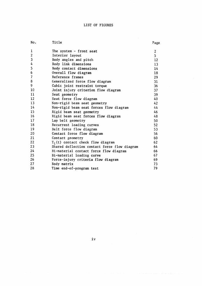
LIST OF FIGURES

No. Title

The system - front seat Interior layout Body angles and pitch Body link dimensions Body contact dimensions Overall flow diagram Reference frames Generalized force flow diagram Cubic joint restraint torque Joint injury criterion flow diagram Seat geometry Seat force flow diagram Non-rigid beam seat geometry Non-rigid beam seat forces flow diagram Rigid beam seat geometry Rigid beam seat forces flow diagram Lap belt geometry Recurrent loading curves Belt force flow diagram Contact force flow diagram Contact geometry Ti (t) contact check flow diagram Shared deflection contact force flow diagram Bi-material contact force flow diagram Bi-material loading curve Force-injury criteria flow diagram Body matrix Time end-of-program test

Page

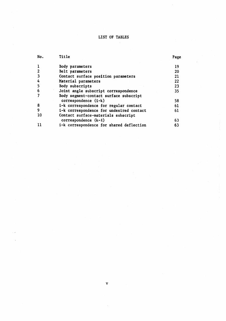
LIST OF TABLES

No. Title

Body parameters Belt parameters Contact surface position parameters Material parameters Body subscripts Joint angle subscript correspondence Body segment-contact surface subscript correspondence (i-k) i-k correspondence for regular contact i-k correspondence for undesired contact Contact surface-materials subscript correspondence (k-R)

i-k correspondence for shared deflection

Page

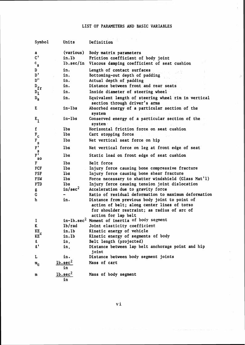
LIST OF PARAMETERS AND BASIC VARIABLES

Symbo 1 Units Definition

F' s F ' S 0 F FCF FSF FSW FTD g G h

(various) Body matrix parameters in,lb Friction coefficient of body joint lb, sec/in Viscous damping coefficient of seat cushion

,.

in, in.

in-lbs

in-lbs

lbs lbs lbs

Length of contact surfaces Bottoming-out depth of padding Actual depth of padding Distance between front and rear seats Inside diameter of steering wheel Equivalent length of steering wheel rim in vertical section through driver's arms

Absorbed energy of a particular section of the sys tem Conserved energy of a particular section of the sys tem Horizontal friction force on seat cushion Cart stopping force Net vertical seat force on hip

lbs Net vertical force on leg at front edge of seat

lbs Static load on front edge of seat cushion

lbs Belt force lbs Injury force causing bone compressive fracture lbs Injury force causing bone shear fracture lbs Force necessary to shatter windshield (Glass Mat' 1) lbs Injury force causing tension joint dislocation in/sec2 Acceleration due to gravity force - Ratio of residual deformation to maximum deformation in. Distance from previous body joint to point of

action of belt; along center lines of torso for shoulder restraint; as radius of arc of action for lap belt

in-lb. sec2 Moment of inertia of body sepent lb/rad Joint elasticity coefficient in, lb Kinetic energy of vehicle in. lb Kinetic energy of segments of body in. Belt length (projected) in. Distance between lap belt anchorage point and hip

joint in. Distance between body segment joints

lb. sec2 Mass of cart in

lb. sec2 Mass of body segment in

Symbol Units Definition

NC NBYLT NBODY NCART NEND NLOAD NOUT P P ' r r A R

- lbs lbs in. in.

s lb/in S in.

sec sec sec sec in.

in. lbs/rad in/sec

lbs

in. in.

x" in.

in,

x in, C

in. in,

Y I' in.

Order of polynomial approximation to loading characteristics of materials and belts

Maximum number of contact surfaces Belt option Occupant option Cart deceleration option End of program option Loading curve option Output variable options Normal contact force Tangential contact force Radius of curvature of body contact arcs Ankle radius Ratio of energy conserved to that absorbed in belt or contact surface Linear spring coefficient at front edge of seat Perpendicular distance from center of body contact arc to contact surface Time Time points at which input data are available Maximum duration of program run

Length of integration time interval Distance of contact point from contact surface reference point, measured along contact surface Linear joint restraint coefficients Tangential velocity of body contact point along contact surf ace Static load on seat cushion at hip joint

Horizontal joint coordinate (inertial) Horizontal joint coordinate (relative to inside of vehicle) Horizontal coordinates of contact surface reference points (noninertial) Horizontal coordinate of hip relative to space fixed axes, with origin of axes at the initial hip position (inertial) Horizontal displacement of center of gravity of vehicle, relative to initial position (inertial)

Initial forward velocity of body and vehicle

Vertical joint coordinate (inertial) Vertical joint coordinate (relative to inside of vehicle) Vertical coordinates of contact surface reference points (noninertial)

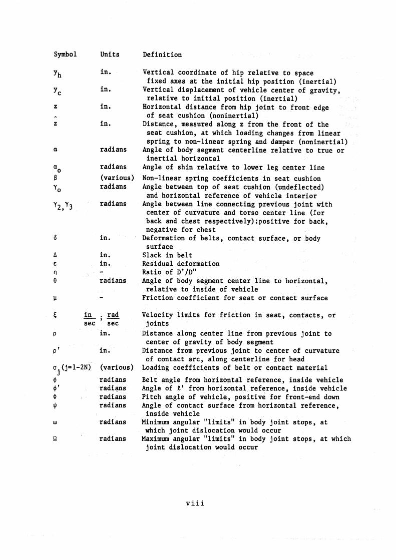
Symbo 1 Units Definition

in.

in,

in.

in.

radians

radians (various) radians

radians

in.

in, in. - radians

5 - in . rad 9 -

sec sec P in.

o ' in.

a. (j=l-2N) (various) 3

4 radians 4)' radians 3 radians JI radians

w radians

51 radians

Vertical coordinate of hip relative to space fixed axes at the initial hip position (inertial)

Vertical displacement of vehicle center of gravity, relative to initial position (inertial)

Horizontal distance from hip joint to front edge of seat cushion (noninertial) Distance, measured along z from the front of the seat cushion, at which loading changes from linear spring to non-linear spring and damper (noninertial)

Angle of body segment centerline relative to true or inertial horizontal

Angle of shin relative to lower leg center line Non-linear spring coefficients in seat cushion Angle between top of seat cushion (undeflected) and horizontal reference of vehicle interior Angle between line connecting previous joint with center of curvature and torso center line (for back and chest respectively) ;positive for back, negative for chest Deformation of belts, contact surface, or body surface Slack in belt Residual deformation Ratio of D' /D" Angle of body segment center line to horizontal, relative to inside of vehicle Friction coefficient for seat or contact surface

Velocity limits for friction in seat, contacts, or joints Distance along center line from previous joint to center of gravity of body segment Distance from previous joint to center of curvature of contact arc, along centerline for head Loading coefficients of belt or contact material

Belt angle from horizontal reference, inside vehicle Angle of R' from horizontal reference, inside vehicle Pitch angle of vehicle, positive for front-end down Angle of contact surface from horizontal reference, inside vehicle

Minimum angular "limits" in body joint stops, at which joint dislocation would occur Maximum angular "limits" in body joint stops, at which joint dislocation would occur

SECTION A, INTRODUCTION

This report is concerned with the mathematical simulation of

the motion of an occupant of a motor vehicle which has been involved

in an accident. There are three phases to this simulation project.

The first phase is quite similar to the Cornell simulation project,

differing only in the methods of obtaining certain quantities and in

the number of allowed body contacts with the vehicle interior. An

Highway Safety Research Institute computer program is currently being

used to generate results which are being compared with results from the

Cornell program.

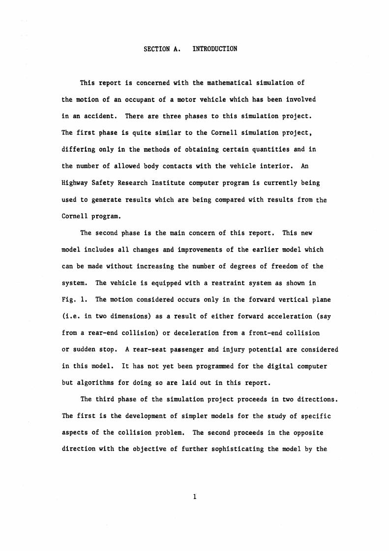
The second phase is the main concern of this report. This new

model includes all changes and improvements of the earlier model which

can be made without increasing the number of degrees of freedom of t:he

system. The vehicle is equipped with a restraint system as shown in

Fig. 1. The motion considered occurs only in the forward vertical plane

(i.e. in two dimensions) as a result of either forward acceleration (say

from a rear-end collision) or deceleration from a front-end collision

or sudden stop. A rear-seat passenger and injury potential are considered

in this model. It has not yet been programmed for the digital computer

but algorithms for doing so are laid out in this report.

The third phase of the simulation project proceeds in two directions.

The first is the development of simpler models for the study of specific

aspects of the collision problem. The second proceeds in the opposite

direction with the objective of further sophisticating the model by the

addition of body elasticity, three-dimensional motion, asymetries, artd

relative vehicle interior motions.

The body of the person is approximated by an eight segment

articulated system of links. The eight angles of these segment center

lines, which are measured counter-clockwise from the true horizontal,

and the two inertial Cartesian coordinates of the hip joint comprise the

ten degrees of freedom of the body in the simulations of phases one

and two. Phase three will have a larger number of degrees of freedom due

to the explicit simulation of such body deformabilities as spine-limb

length, shoulder joint motion, and chest-face-abdomen deformations. The

phase one program and Cornell ignore these deformabilities while the

phase two simulation approximates them by the introduction of injury

criteria based on forces. The chest-face-abdomen deformabilities are

further approximated by the use of force-deflection loading curves which

modify their contact or belt forces. See Section C.4.e and C.4.f for details.

These injury criteria can also be used as end-of-program tests, with a

program option to specify which of these criteria would be so used, These

will be enumerated below. In phases two and three, each of the seven joints

of the body is considered to possess torsional elasticity proportional to

the relative joint angle, Coulomb friction, and 2-sided angular restraints

approximating actual limitations to joint motion. Cornell allows elasticity

for only the two spinal joints, with two-sided linear restraints for the

neck and spinal joints and one-sided linear restraints for the elbow

and knee. The phase one program adds a two-sided linear restraint

for the shoulder and a one-sided one for the hip. The phase two

simulation allows the form of the restraints to be linear, cubic, or

arbitrary. Again an option in the computer program will specify which

of these would be used, See Section C.4.c for details.

The vehicle of phase one and the Cornell vehicle possess one degree

of freedom, This is straight-line horizontal motion. Vertical motion

and pitch are included in the models of phases two and three. In the

former simulation an option exists which specifies whether this horizontal

acceleration has an arbitrarily specified time history or whether a cart-

stopping-mechanism is used as would be the case with a sled test. The

phase two simulation has no such option and all three accelerations must

be known time-functions, However, it is possible to include tables for

the horizontal, vertical, and angular positions and/or rates as input data

and thus eliminate some or all of the vehicle integrations, The phase

three simulation will have the option of using explicit differential

equations for the three vehicle variables, a three-dimensional cart-stopping-

mechanism, or the above tabular data.

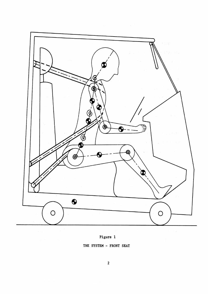
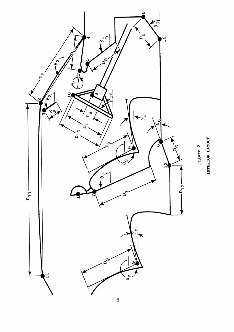
The vehicle interior is described by taking several vertical sections

through the vehicle, through the center of the occupant, through his legs,

and through his arms, These sections are then superimposed to form one

composite interior layout, as shown in figure 2. All three phases have

an option to specify the position of the person in the vehicle, whether

driver, front-seat passenger or rear-seat passenger. Cornell specifies

only driver or front-seat passenger by the values of certain contact

surface parameters. The Cornell vehicle interior contains only seven

contact surfaces, all of which are flat. The phase one program has twelve

flat surfaces, while phases two and three have seventeen, some of which

may be curved. Cornell considers only seven combinations of contact

between particular body segments and contact surfaces. The number of

possible contacts in the Highway Safety Research Institute simulations

varies with the position of the occupant in the car. In the phase one

program the driver has 11 possible contacts, the front-seat passenger 14,

and the rear-seat passenger 13, In phases two and three these numbers

are 20, 18 and 14 respectively.

The Cornell contact surfaces are assumed to consist of a single

material, This is also the case in the phase one program, In phases

two and three some of the contact surfaces may be padded, as indicated

in Table 10. Cornell and the phase one program have only rigid (non-

movable) contact surfaces, while in phase two the motion of the non-rigid

ones (for example, the sunvisor, steering wheel rim and column, and head

rest) is approximated by force-deflection loading curves and the use of

the shared deflection subroutine (Fig, 23). In phase three the non-rigid

motion will be expressed in terms of explicit differential equations, All

these force-deflection loading curves are assumed to be expressed by

fifth-order polynomials in both the deflection and the rate of deflection.

Cornell and the phase one program represent the seat by two systems,

one a linear spring whose force acts at the front edge of the seat and the

other a linear damper - third order non-linear spring combination whose force acts at the hip joint. Thus this latter force may move along the

seat following body motion and might overlap the front edge force, This

overlap is prevented in phases two and three either by logic or by using

an entirely different seat representation, two possibilities for which are a

rigid beam supported by the present spring-damper systems and a pair

of non-rigid beams. In all cases, logic allows the person to fall

completely off the seat. Logic in the appropriate sections of the

simulations of all three phases automatically differentiates between

a person whose feet touch the floor and a child whose legs stick straight

out in front of him,

In all cases, the restraint system is composed of a lap belt whose

force acts at a constant radial distance from the hip joint and a shoulder

restraint whose two forces act at specified points on the body torso

center lines. Cornell has an option to specify whether the 3 belt sections

and thus the three belt forces are independent, whether the lap belt is

independent of the shoulder restraint while the tension forces in the

two sections of the shoulder restraint are equal, or whether the forces

in all three sections are the same. The phase one program and the phase

two simulation assume that the first of these alternatives is true. Phase

three will have this option. All three phases have another option to

specify how many of the belts are in use, whereas Cornell must use the

values of the various belt parameters to do this. The phase one p1:ogram

assumes that the chest wall and abdomen do not deform, while phase two

approximates their deformation by load-deflection curves and a shared-

deflection subroutine to generate the belt forces. Phase three will have

explicit differential equations for their motion,

Cornell and the phase one program do not consider injuries at all,

In phase two, the injuries which are considered in the first approximation

for non-rigid body segments are joint dislocations, bone fractures, and

cuts. Joint dislocations can be of two types; one caused by excessive

relative angle and the other by excessive tensile forces across thie joint.

Fractures are also of two types; one caused by excessive compressive

force along the center line of the bone, the other by excessive shear

forces. This last type affects not only the spine and limbs, but also

the skull, face, and ribs. Cuts are considered only for head-windshield

contact when the glass is actually shattered. These injury criteria

will also appear in phase three, though perhaps in different forms.

For all three phases the equations of motion for the system are

obtained from the system Lagrangian, which includes the system kinetic

energy, potential energy, dissipated energy rate, and the classical

generalized non-conservative forces.

SECTION B.

Derivation of Matrix Equation

m -+ -+ -+

The body matrix equation, Az = b, where z i s the generalized (-0-

o rd ina te vector with the ten components a through a 1 8' Xh

and yh; A i s

-+ the body matrix a s shown i n sec t ion C, 5; and b i s the generalized force

vector whose components a r e calculated i n sec t ion c.4, i s obtained from

the system Lagrangian:

d a (KE) + 2 (PE) + 3 (DE) - - ;ii [ ail, a R~ a zi ati - FZi, f o r i = 1-10,

where KE i s the system k ine t i c energy, PE i s i t s po ten t i a l energy, DE

i s i t s d i ss ipa ted energy r a t e , and the FZi a r e the c l a s s i c a l generalized

forces , developed i n d e t a i l i n sec t ions C.4. e and C . 4. f . The t o t a l body k ine t i c energy i s

where m . and I . a r e the mass and moment of i n e r t i a of the i - t h body se- 1 1

gment, respect ively, a is the angle of the i - t h body segment center i

l i n e to t he t rue o r i n e r t i a l horizontal measured counter-clockwise, and

Xi, Y . a r e the i n e r t i a l coordinates of the center of gravi ty of the i - t h 1

body segment a s follows:

. . X1 = x - p a s ina

h 1 1 1

I I

Y1 = y + p a cosa h 1 1 1

. X2 = x + L cosa + p cosa -

h 1 1 2 2 a2 - ih - L a sinal 1 1

- p2A2 s ina 2

Y 2 = y + L s ina + p 2 s ina2 f = ih + L ~ ; L ~ cosal + p2U2 cosa h 1 2

X3 = xh + L cosa + L2 cosa2 + p 3 cosa 1 1 3

= y + L s ina + L s ina2 + p 3 sins Y3 h 1 1 2 3

i3 = ;h - L a s ina - L a s ina2 - p 3 i 3 s ina3 1 1 1 2 2

i3 = ih + L ~ ; L ~ cosa + L a cosa2 + p3a3 COSa3 1 2 2

X4 = x + L cosa + L cosa2 + L3 cosa3 + p 4 h 1 1 2 c0sa4

- + L s ina + L s ina2 + L s ina + p s i na4 Y4 - Yh 1 1 2 3 3 4

. . . . . X4 = xh -L a s ina -L a s ina -L a s ina 1 1 1 2 2 2 3 3

-p4a4 s ina4

cosal + L2a2 cosa2 + L a cosa + p4a4 3 3 3 ' cosa4

X5 = x + L cosal + L cosa2 + L cosa + p h 1 2 4 3 5 C0Sa5

- + L s ina + L s ina + L s ina Y5 - Yh 1 1 2 2 4 + p 5 s i na 5 . .

X = x -L a s ina -L a s ina -L a s ina 5 h 1 1 1 2 2 2 4 3 -p5a5 s ina 5

. e

Y5 = yh + Llal cosa + L a cosa + L a cosa 1 2 2 2 4 3 + p5A5 cosa 5

X6 = xh + L cosa + L cosa + L4 cosa + L cosa + p 6 cosa6 1 1 2 2 3 5 5

- + L s ina + L s ina + L s ina + L s ina '6 - Yh 1 1 2 2 4 3 5 + p 6 s ina6

. . . . - -L a s ina -L a s ina -L a s ina + L a s ina -p a s ina %5 - ;h 1'1 1 2 2 2 4 3 3 5 5 5 6 6 6

. . Y6 = y + L n cosa + L a cosa + L a cosa + L a cosa +p a

h 1 1 1 2 2 2 4 3 3 5 5 5 6 6 'OSa6

. - X7 = xh + p 7 cosa 7 X7 - xh -p7a7 s ina7

- + L cosa + p cosag . , '8 - 'h 7 7 8 X = x - L a s ina -p a si.na 8 h 7 7 7 8 8 8

. Y8 = x + L s ina + p s inag

h 7 7 8 i = ; + L ;

8 h 7 7 cosa7 + p8a8

c0 "8

Figures 3 , 4 and 5 show the body dimensional parameters and angles; L o i s IL

the l i n k length, p i the dis tance from the previous j o i n t t o the center of

grav i ty , and a . a s above. In f i gu re 3 the axes shown with broken l i n e s 1

a r e the t rue , outs ide, or i n e r t i a l horizontal and v e r t i c a l reference:;,

while the so l id l i n e axes a r e r e l a t i v e to the i n t e r i o r of the vehiclle and

a r e thus inclined a t an angle 0 to the i n e r t i a l axes. This angle 0 i s

the vehic le p i t ch angle and is pos i t ive f o r a vehic le having i t s f ront

end down. The angles of the body segment center l i n e s with the vehic le

i n t e rna l horizontal reference ( i . e . the f l oo r ) a r e equal to the i n e r t i a l

angles plus the vehic le p i tch angle; i . e . 0 = a + a . If the vehic le i i

does not p i tch , then the reference frames w i l l coincide. In a l l cases,

xh and yh a r e the i n e r t i a l coordinates of the hip jo in t .

The poten t ia l energy due to j o in t e l a s t i c i t y , the s ea t springs (both

l i nea r and third-order non-linear) and gravi ty , respect ively, i s :

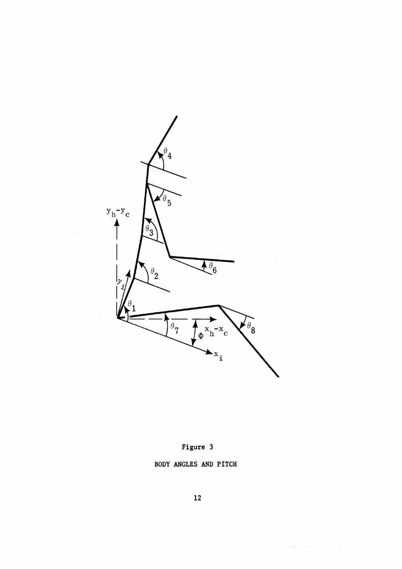
Figure 3

BODY ANGLES AND PITCH

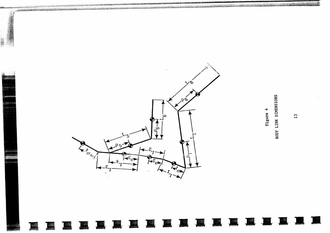
Figure 5

BODY CONTACT DIMENSIONS

14

where yl and y z a r e a u x i l l i a r y va r i ab l e s t o be defined i n s ec t ion C.4.d.

In general , p o t e n t i a l energy i s the i n t e g r a l of t he fo rce o r torque

over t he d i s t ance ( l i n e a r o r angular) involved. Since these a r e a l l

wel l defined funct ions i n the ana lys i s , they can a l l be d i r e c t l y in-

tegra ted ; even the s e a t non-linear spr ing , which gives

However, i f e i t h e r of t he other two s e a t representa t ions a r e used,

appropriate terms must be subs t i t u t ed .

The d iss ipa ted energy r a t e due t o s e a t f r i c t i o n , the s e a t damper,

j o i n t f r i c t i o n , and t h e j o i n t r e s t r a i n t s , respec t ive ly , i s :

In each case here, the r a t e of energy d i s s i p a t i o n i s equal t o t h e i n t e g r a l

of the fo rce or torque over t he ve loc i ty ( l i nea r o r angular) . I n

p a r t i c u l a r i f t h e j o i n t r e s t r a i n t s ( s ec t ion C.4.c. and Fig. 9) do not

depend on the angular r a t e s , they could be in tegra ted yielding:

The FZi a r e obta ined by f i n d i n g t h e e x t e r n a l f o r c e s and moments

c o n s i s t i n g of t h e t h r e e b e l t f o r c e s , t h e normal and t a n g e n t i a l c o n t a c t

f o r c e s , and t h e p i t c h . (Sect ions C.4.e. and C . 4 . f . ) .

A f t e r d i f f e r e n t i a t i o n and proper a l g e b r a i c manipula t ion, t h e r e

r e s u l t s a s e t of t e n d i f f e r e n t i a l equat ions i n t h e t e n genera l i zed

+ -+ coord ina tes , which can be recognized a s A z = b, where A i s a f u n c t i o n of

+- -b +- +- -+ z and b of z and z. For e a s e of c a l c u l a t i o n b i s r e p a r t i t i o n e d i n t o

those i tems c a l c u l a t e d i n Sec t ion C.4.

SECTION C.

SIMULATION

The detailed simulation presented in this section is that of

phase two. It incorporates all the additions and changes that can

be made to the phase one program without raising the number of degrees

of freedom of the system. The overall flow chart for the phase two

simulation program is shown in figure 6,

SECTION C.1

INPUT INFORMATION

The general format for the input information is that the various

parameters should be grouped according to type. This arrangement allow

any one section to be changed by simply substituting new data cards.

A complete list of parameters and the basic variables along with their

units and definitions will be found just before the introduction, section A.

Arbitrarily specifiable initial conditons are: body position

angle (O through O ), belt length (k ) and angle ( 4 ) for j = 1 10 80 j 0 .I 0 . through 3, vehicle velocity (X ) .

CO

Vehicle pitch angle, plus its rate and acceleration, and deceleration

time-histories are entered in tabular form, as well as vehicle velocity

e

((t,), Xc(tm), ;,(tm), ((t,) if available, for all t 1 The only other m

vehicle parameters needed at present are its mass (mc) and moment of

inertia (I,),

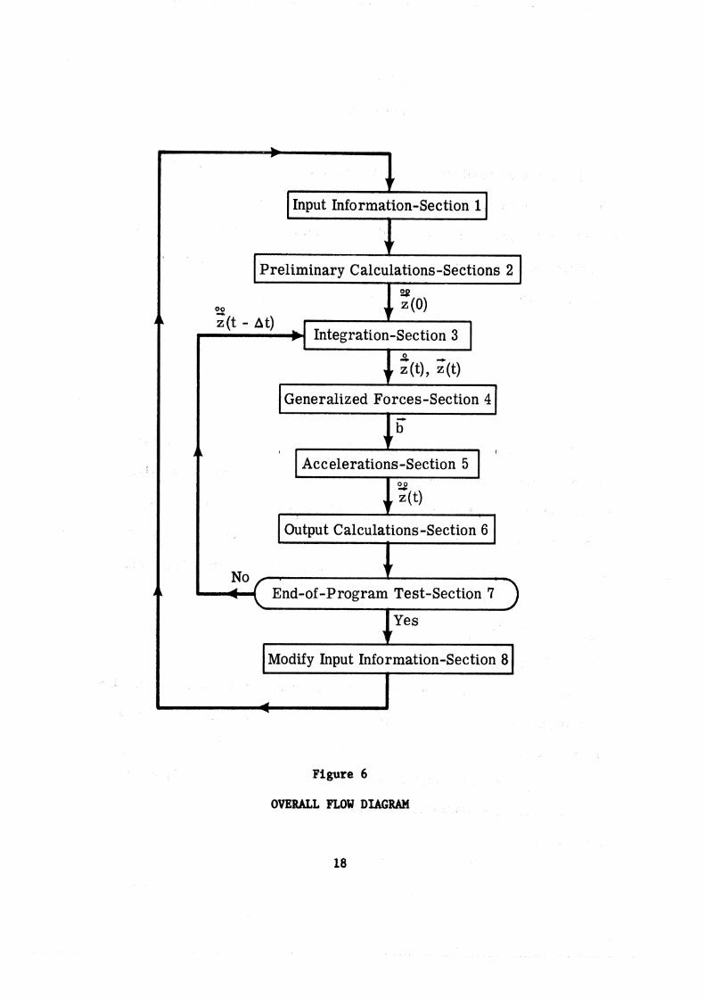
Figure 6

OVERALL FLOW DIAGRAM

subscript - i 1 2 3 4 5 6 7 8 9 10 other

contact radius r

mass I X X X X X X X X

x x x x x x x x x x rA

shear fracture force

inertia I I X X X X X X X X

F S F x x x x x x x x x

length L ~ x x x x x x x x

center of gravity distance P x x x x x x x x

tension dislocation force F T D x x x x x x x

compression fracture force FCF x x x x x x x

coulomb friction coefficient C ' x x x x x x x

elasticity K

minimum joint angle u l x x x x x x x

x x x x x x x

friction velocity 1 imi t E

maximum joint angle SI x x x x x x x

x x x x x x x

linear Joint stop7 ( T I I x x x x x x x

coefficients i I x x x x x x x

center of curvature distance P

TABLE 1.

center of curvature angle from center- line Y x x

<

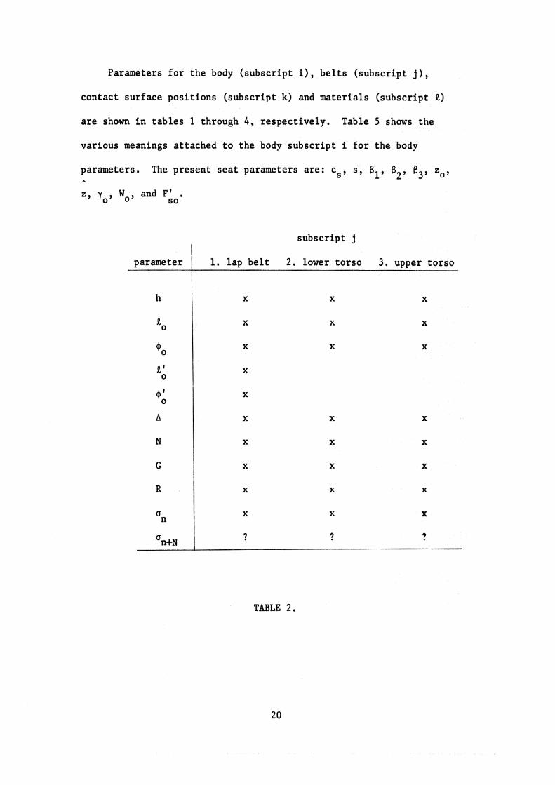
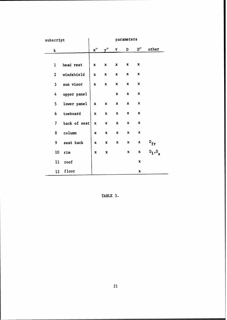
Parameters for the body (subscript i), belts (subscript j),

contact surface positions (subscript k) and materials (subscript L)

are shown in tables 1 through 4, respectively. Table 5 shows the

various meanings attached to the body subscript i for the body

parameters. The present seat parameters are: cs, s, Bl, B 2 , B3, z0, A

z , yo, Wo, and F' . s 0

subscript j I

TABLE 2 ,

parameter

h

1. lap belt 2. lower torso 3. upper torso

x x X

X X X

subscript I parameters

1 head rest x x x x x

2 windshield x X X X X

3 sun visor x x x x x

- k

upper panel I

x1! y" Y D D" other

lower panel

toeboard 1 back of seat

seat back

floor I

X X x

x x x x x

x X X X x

x x x x x

x x x x x

x x x x x

X X X X

X

X -

TABLE 3 .

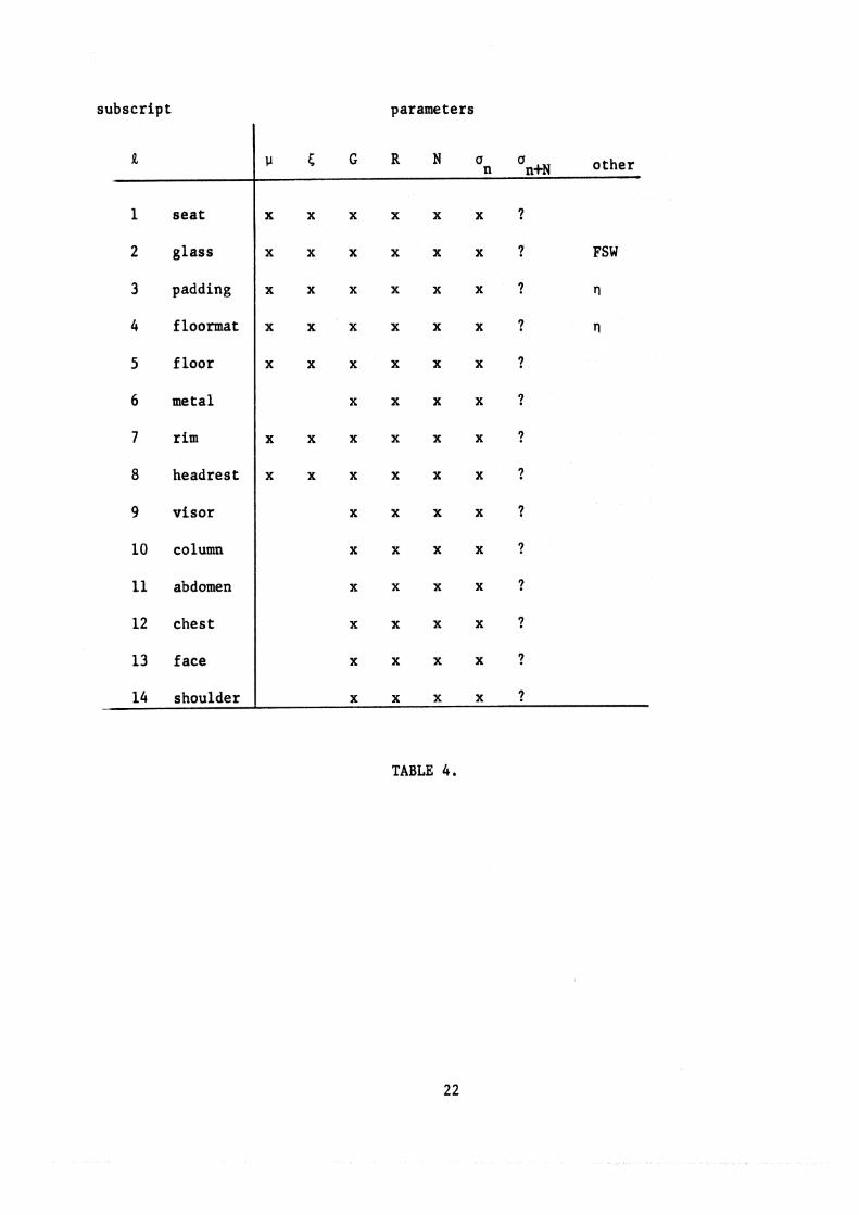
subscript parameters

1 seat

2 glass

3 padding

4 floormat

5 floor

6 metal

7 rim

8 headrest

9 visor

10 column

11 abdomen

12 chest

13 face

14 shoulder

x x x x x x ?

x x x x x x ? FSW

X X X X X x ? n

X X X x x x ? n

X X x x x x ?

X X X X ?

X X X X X x ?

X X X X X x ?

X X X X ?

X X X x ?

X X X X ?

X X X x ?

X X X X ?

X X X X ?

TABLE 4 ,

subscr ip t bone in ju ry c r i t e r i a

i body contact shear compress:Lon seamen t jo in t a r c f r a c t u r e f r a c t u r e

parameters

cen te r lower upper cen t e r cen t e r t o r so spine back spine spine

m,I,L,p G I K T 1 9 G p ' ,y FSF FCF T' ,w,Q, 5, FTD

1

upper upper ches t upper upper t o r so spine spine spine

lower h ip lower lower lower t o r so back spine spine

I h e a d neck head s k u l l

upper shoulder shoulder back arm

upper arm

lower elbow elbow r i b lower arm arm

upper knee knee upper upper l eg l e g l eg

foo t lower lower l e g leg

8

1 sh in face

lower l eg

lo 1 hand -

TABLE 5.

SECTION C.2

PRELIMINARY CALCULATIONS

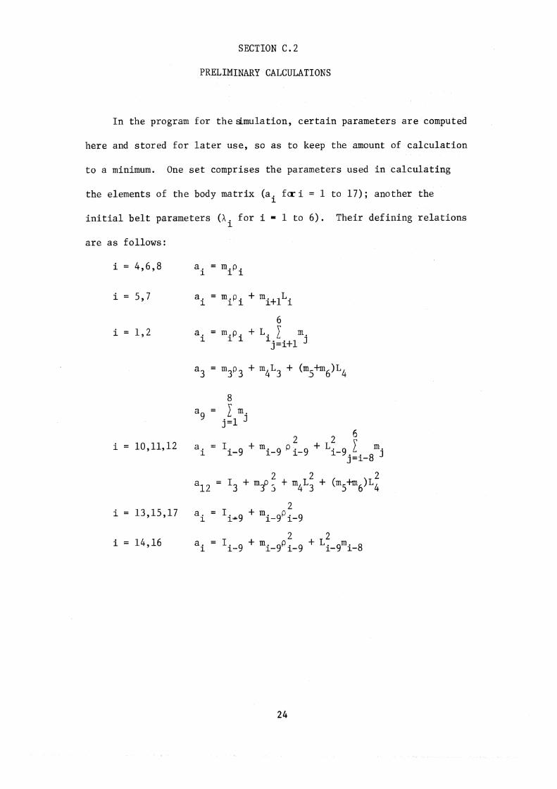
I n t h e program f o r thes imula t ion , c e r t a i n parameters a r e computed

here and s t o r e d f o r l a t e r use , so a s t o keep t h e amount of c a l c u l a t i o n

t o a minimum. One s e t comprises t h e parameters used i n c a l c u l a t i n g

t h e elements of t h e body m a t r i x (ai f c r i = 1 t o 1 7 ) ; another t h e

i n i t i a l b e l t parameters (hi f o r i = 1 t o 6 ) . Their d e f i n i n g r e l a t i o n s

a r e a s fo l lows :

h 4 = L cosO + h2cos0 1 l o 20 - k20C0s+20

= L cosO + L cosO + h cosO '6 1 l a 2 20 3 3 0 ~ ~ 3 0 C O S ~

30

Single parameters a r e the i n i t i a l l ap b e l t angle and length, and t h e

angle between the s h i n sur face and the lower l e g center l i n e . These

a r e def ined, respec t ive ly , as :

-1 = 4 + s i n [h,la;l,

$10 0

a o = sin-'[ (r7-rA) 1 ~ ~ 1 .

Other ca l cu la t ions performed here a r e of the i n i t i a l values of

t h e output da t a va r i ab l e s . Most of these w i l l be zero; eg the head

and ches t acce l e ra t ions a t t h e i r cen ters of grav i ty , a l l energies

except k i n e t i c , and a l l contac t forces except those on on the s e a t

back, head r e s t , f l o o r , and toeboard. I n i t i a l k i n e t i c energies a r e ,

respec t ive ly f o r the veh ic l e and body segments:

1 K E ~ = Ti ;ao, f o r i = 1-8.

I n i t i a l contact forces a r e dependent on i n i t i a l body pos i t i on (or

perhaps v i c e versa,using the appropr ia te loading r e l a t i o n f o r fo rce

i n terms of de f l ec t ion with r a t e of de f l ec t ion equal t o zero) .

L a s t l y t h e i n i t i a l a c c e l e r a t i o n s on t h e body a r e c a l c u l a t e d

cons ider ing on ly t h e i n i t i a l f o r c e s due t o g r a v i t y , t h e b e l t s , and

t h e i n i t i a l c o n t a c t s . The genera l i zed c e n t r i f u g a l f o r c e s , j o i n t

to rques , and n e t s e a t cushion f o r c e s a r e a l l zero .

The v e h i c l e i n i t i a l a c c e l e r a t i o n s a r e read from t h e t a b l e s .

SECTION C.3

INTEGRATION

At present, a four point Adams-Moulton method started with a

modified Euler method is used. The Euler method is used to obtain

the first three points after the given initial point, Thereafter

four points are used in the Adams third difference prediction and

correction equations, At each computation of a new point, the

iteration continues until successive approximations are within a

given tolerance or the iteratian has been tried a prescribed number

of times.

With an integration option, different schemes could be chosen

according to the option. Otherwise the integration would be (and is)

carried out by a subroutine.

If, in the input information, tabular data is available only

for Kc l tm) , yc ($), and B (tm) , then these must be integrated for the vehicle position and velocity and for its pitch angle and rate. If

tabular data is also available for xc(tm), iC(tm), i(tm) andlor for

xc (tm) , yc (t,) , O(t,), some or all of the integratiols for the

vehicle may be omitted and the proper values read in from the table.

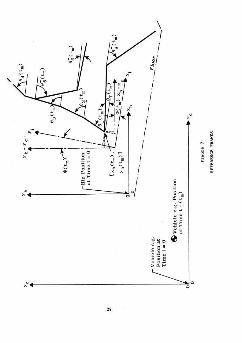
The body generalized coordinates (xh, yh, a1 - a8) are now in the

inertial reference frame and can be directly integrated twice, The

body angles and rates relative to the vehicle interior [ei(t+At),

Bi(ttbt)] are obtained by adding 4 ( t ~ 1 ) and i(tel) to a(ttAt) and

& (tt~t) respectively.

Figure 7 shows the various reference frames, along with the

vehicle center of gravity and body positions at some later time t-t,.

SECTION C. 4

GENERALIZED FORCES

Once the set of ten equations in the ten generalized coordinates

is obtained for the body motion (see Section B for details), it can

be separated so that all the acceleration terms are on one side; i.e. L l i .

-b AZ = 9, where A is a function of z and $ of t and Z. In order to -+

facilitate the calculation of the components of the vector b, which is

now called the generalized force vector, it is partitioned into sections

for the forces and moments due to: 1) centrifugal force, 2) gravity,

3) joint torques, 4) the seat cushion, 5) the belts, and 6) contacts

with the interior surfaces of the vehicle, as shown in Fig. 8. In

order then,

= C - Gi + J + Si + B + Qi, for i 1 to 10. bi i i i

-+ The vector z has as components a through a

1 8 9 Xh, and y h '

In the present case, when the magnitude of the vehicle deceleration

is known for each time point, the magnitude of the resulting force on

the vehicle is simply:

The instantaneous positions and velocities of the seven joints,

relative to the inside of the vehicle, are needed in several of the

subsequent sections. They are calculated from the following relations.

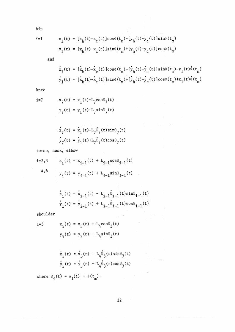
hip

i= 1 xl(t) = Ixh(t)-xc(t) lcos@(tm)-[~h(t)-~c(t) lsinm(tm)

yl(t) = [xh(t)-xc(t)lsin@(tm)+[yh(t)-yc(t)1cos~(tm)

and

$(t) = [Gh(t)-ic(t) lcos~ (tm)- [ih(t)-ic (t) I sin@ (tm)-yl(t)i (tm)

il(t) = ~~h(t)-~c(t)lsin@(tm)+l~h(t)-~c(t)l~~~~(t,)+~l(~)~(tm)

knee

i= 7 x7(t) = x (t)+L cos07(t) 1 7

y7(t) = y1(t)+L7sinO7(t)

i7(t) = xl(t)-~ 7 6 7 (t)sino7(t)

i7(t) = ;1(t)+~767 (t)cOso7 (t)

torso, neck, elbow

i=2,3 xi(t) = x i 1 + Li-l~~~Oi-l(t)

496 y,(t) = Yi- 1 (t) + Li-lsinO (t) i- 1

shoulder

i=5 x 5 (t) = x3(t) + L4cos03(t)

y5(t) = y3 (t) + L4sin03(t)

. . x 5 (t) = xj(t) - L403(t)sin03(t)

G5(t) = ;3(t) + L 4 Q 3 (t)coso3(t)

SECTION C. 4. a

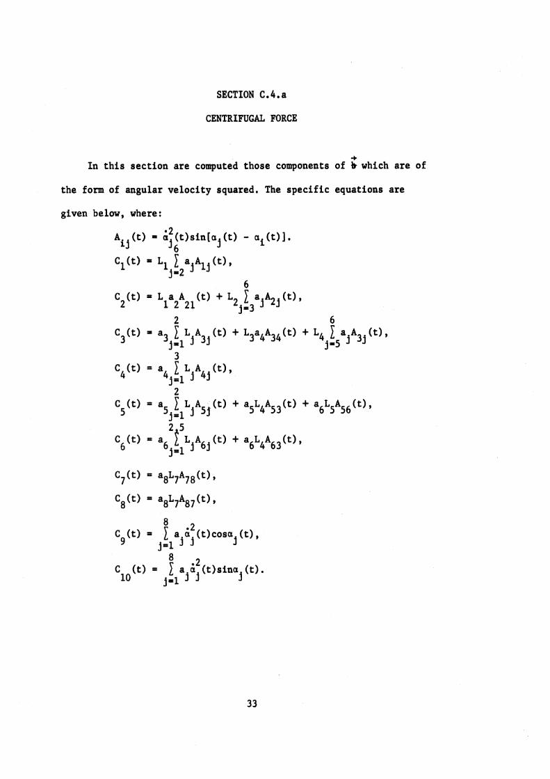
CENTRIFUGAL FORCE

-b In this section are computed those components of b which are of

the form of angular velocity squared. The specific equations are

given below, where:

Aij(t) = i2(t)sin[a (t) - ai(t)]. j 6 J

cl(t) = L~ 1 a j ~ l j (t), .iu2

6 = L a A (t) + LZ 1 ajA2j(t),

C2(t) 1 2 2 1 j = 3

.2 Cg(t) ' 1 . a (t)cosa (t),

jP1 j .I j

SECTION C . 4 . b

GRAV I TY

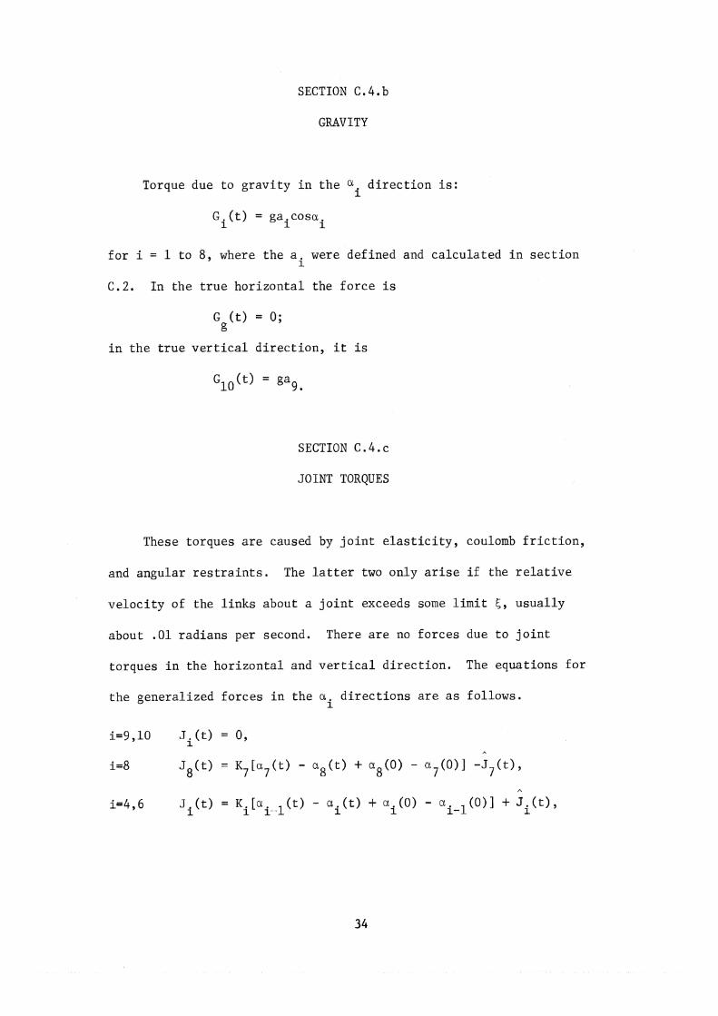
Torque due t o g r a v i t y i n t h e a d i r e c t i o n i s : i

G . ( t ) = gaicosai 1

f o r i = 1 t o 8 , where t h e a . were de f ined and c a l c u l a t e d i n s e c t i o n 1

C.2. I n t h e t r u e h o r i z o n t a l t h e f o r c e is

G ( t ) = 0 ; g

i n t h e t r u e v e r t i c a l d i r e c t i o n , i t i s

SECTION C . 4 . c

JOINT TORQUES

These to rques a r e caused by j o i n t e l a s t i c i t y , coulomb f r i c t i o n ,

and angu la r r e s t r a i n t s . The l a t t e r two on ly a r i s e i f t h e r e l a t i v e

v e l o c i t y of t h e l i n k s about a j o i n t exceeds some l i m i t 5 , u s u a l l y

about . 0 1 r a d i a n s per second. There a r e no f o r c e s due t o j o i n t

to rques i n t h e h o r i z o n t a l and v e r t i c a l d i r e c t i o n . The equa t ions f o r

t h e genera l i zed f o r c e s i n t h e a d i r e c t i o n s a r e a s fo l lows . i

i=4,6 J . 1 (t) = K i [ a i l ( t ) - a i ( t ) + a i m - ( o ) ] + J i ( t ) ,

i = 1 , 2 , 5 J i ( t ) = (K.. x + Ki+l)[ai(0) - a i ( t ) l + Ki+l[ai+l(t)-ai+l(0)l n

+ Ki[a,(t)-am(0)l + J i ( t ) - J i+ l ( t ) ,

i= 7 J , ( t ) = K [a ( t ) - a 7 ( t ) + a 7 ( 0 ) - a 8 ( 0 ) l - K1[a7(t) - a l ( t ) + al(0) 7 8

where f o r i = 1-7: A

~ . ( t ) 1 = o f o r ifii(t) - i ( t ) / < ~ ~ ,

i i ( t ) = c f s g n [ ; ( t ) - a . ( t ) ] + T. ( t ) o the rwise . 1 m 1 1

The s p e c i f i c form of t h e angu la r r e s t r a i n t to rques may v a r y ,

bu t i t s genera l form i s shown i n F ig . 9 . The s i m p l e s t and most

u s u a l l y used form is l i n e a r . An a c t u a l r e s t r a i n t curve f o r t h e upward

motion of t h e lower l e g about t h e knee j o i n t , a s found by J . W. Smith

( r e f . 4 ) , i s a l s o shown i n F i g . 9 . A cub ic f i t s t h i s curve q u i t e w e l l .

Table 6 shows t h e j o i n t a n g l e s u b s c r i p t correspondence.

TABLE 6

One of t h e i n j u r y c r i t e r i a used a s a n end-of-program t e s t can be

app l ied here . This i s j o i n t d i s l o c a t i o n due t o excess ive r e l a t i v e

ang le . Its flow diagram i s shown i n F i g . 10.

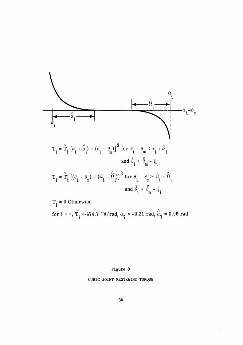
A A 3 A T = T . [a. + cu.) - (6 - 6' ) ] f o r 6 - 6 < a . + cu

i 1 1 1 i m i m l i

and i. < - ti 1 m

A A 3 A T = TI [ ( B - dm) - (Q - Q.)] f o r Bi - 6 > R - R

i l i i 1 m i i

and i. > + 6 1 m i

T = 0 Otherwise i

A A f o r i = 7, T. =-474.7 "#/rad, a7 = -0.21 rad, cu7 = 0.56 r ad

1

Figure 9

CUBIC JOINT RESTRAINT TORQUE

SECTION C.4.d

SEAT FORCES

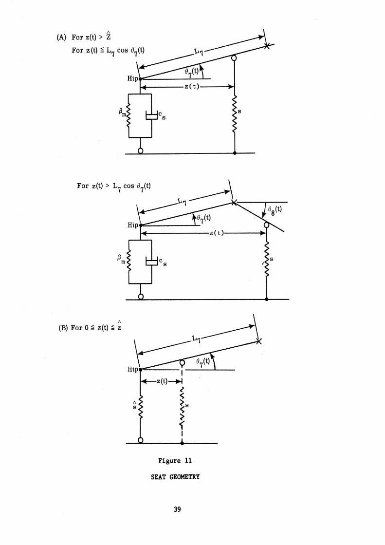
The present representa t ion of the s e a t i s t h a t i t i s composed of

a l i n e a r spr ing whose fo rce a c t s v e r t i c a l l y on the upper o r lower leg

a t t he f r o n t edge of the s e a t , plus a nonlinear spr ing and l i n e a r

damper whose combined force a c t s v e r t i c a l l y on the h ip j o i n t . This i s

the i n t e r i o r v e r t i c a l , not the t rue d i r ec t ion . There is a l s o f r i c t i o n

proport ional t o t h e i r sun which a c t s hor izonta l ly (a l so n ~ n i n e r t i a l l ~ )

a t the h ip j o i n t . Logic i n the simulation allows f o r f a l l i n g off the

s e a t , d i f f e r e n t i a t e s between adu l t s and ch i ldren , and prevents the

overlapping of the two types of forces . This l a s t i s accomplished by A

assuming t h a t , a t some d is tance z from the f ron t edge of the s e a t , i t s

representa t ion changes from t h i s combination t o a l i n e a r spr ing whose

spring constant i s dependent on the conditions a t the previous time

in s t an t . Figure 11 depic ts these various cases; f i gu re 1 2 shows the flow

diagram by which the ne t forces on the body a r e ca lcu la ted f o r each

case. The parameter y has already been defined and ca lcu la ted i n Z O

Section C.2. The generalized fo rce equations i n terms of these ne t

s e a t forces plus the f r i c t i o n a r e a s follows:

Si( t ) = 0 f o r i = 1-6,

(A) For z(t) > % For z (t) 5 L,

For ~ ( t ) > L7 cos e7(t)

Pm

A (B) For 0 2 z(t) 2 z

Figure 11

SEAT GEOMETRY

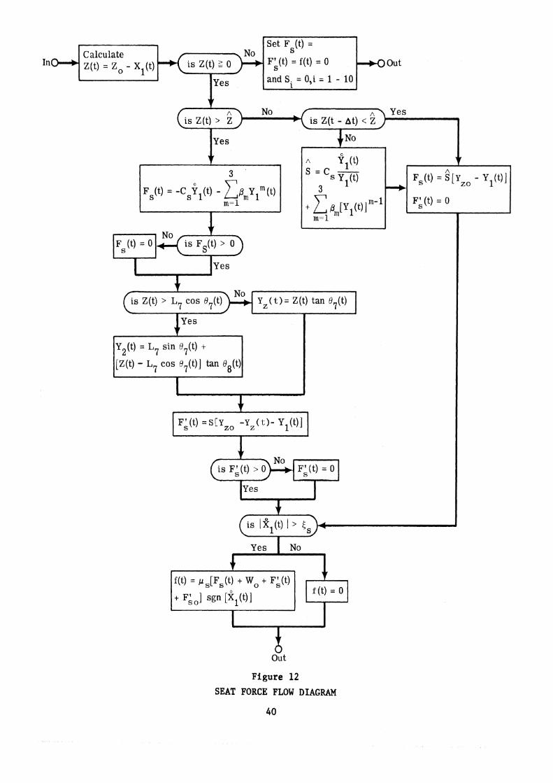
Figure 12 SEAT FORCE FLOW DIAGRAM

where, f o r z ( t ) 2 L7coso7( t ) ,

- - - -cos@(t,) t a n 0 7 ( t ) , - a% - - s i n @ ( tm) tan07 ( t ) ax

h a ~ h

and f o r z ( t ) L7cos 7 ( t ) ,

- - - -cos@ ( tm) t a n 0 8 ( t ) , - a% = s i n @ ( t ) tan08 ( t ) , axh aYh m

where Oi(t) = ai.(t) + @ ( tm) . Another method of prevent ing over lap is t o change t h e repre-

s e n t a t i o n of t h e s e a t t o be e i t h e r t h a t of a non-rigid beam o r t h a t

of a r i g i d beam supported a t f i x e d p o i n t s by t h e p r e s e n t s p r i n g and

spring-damper systems. I n both c a s e s t h e equa t ions of motion w i l l

be d i f f e r e n t .

Another p o s s i b l e r e p r e s e n t a t i o n f o r t h e s e a t cushion is t h a t of

a non-rigid beam. In p a r t i c u l a r i t w i l l be assumed t o c o n s i s t of a

p a i r of uniform beans; one of l e n g t h R and supported a t both ends and

t h e o t h e r of l e n g t h kR c a n t i l e v e r e d a t a f i x e d d i s t a n c e equa l t o i ts

l e n g t h from t h e f r o n t edge of t h e o t h e r beam and t h u s of t h e s e a t .

The two beams and t h e r e s u l t i n g system a r e dep ic ted i n f i g u r e 13.

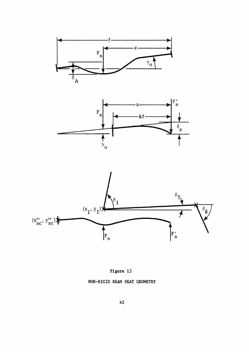
Figure 13

NON-RIGID BEAM SEAT GEOMETRY

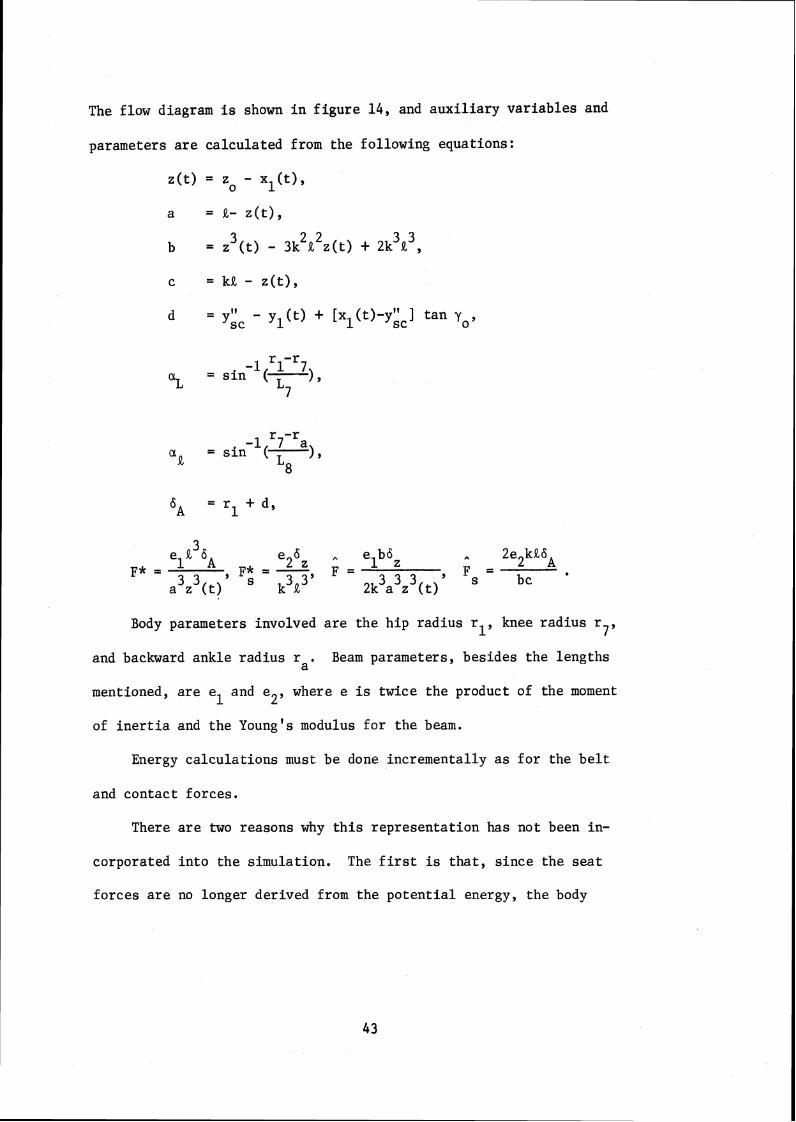
The flow diagram i s shown i n f i g u r e 1 4 , and a u x i l i a r y va r i ab l e s and

parameters a r e ca lcu la ted from the following equations:

r -r -1 7 a

a R

= s i n (- ) 9

8

3 ela 6~ e26z A elbsz 2e2kR\ F* = , F* = - F =

3 3 3 , F =

a3z3(t) s k3R3' 2k a z ( t ) s bc *

Body parameters involved a r e the h ip rad ius rl, knee rad ius r 7 '

and backward ankle rad ius ra. Beam parameters, besides the lengths

mentioned, a r e e and e2 , where e i s twice the product of the moment 1

of i n e r t i a and t h e Young's modulus f o r the beam.

Energy ca l cu la t ions must be done incrementally a s f o r the b e l t

and contac t forces .

There a r e two reasons why t h i s representa t ion has not been in-

corporated i n t o the simulation. The f i r s t i s t h a t , s i nce the s e a t

forces a r e no longer derived from the po ten t i a l energy, the body

I Calculate z(t), a, b, c, d I

T

is z(t) > k l

F, (t) = F* Out

Out

* A I QL1 41 6*1 F , I Calculate

Figure 14

NON-RIGID BEAM SEAT FORCES FLOW DIAGRAM

I 6 = d + zo tan yo z

+ r1 sec [07(t) - aL]

- z(t) tan [8?(t) + uL]

Calculate 6 = d t z, tan yo t L7 sec [08(t) + uk 1 z

- L7 sin $(t) - [z(t) - L7 cos 07(t)] tan [o8(i.) + + c a l c u l a t F f , b .

equa t ions would have t o be re-der ived. The second is t h a t exper imental

conf i rmat ion and numerical d a t a a r e a s y e t l ack ing .

A second p o s s i b l e a l t e r n a t e r e p r e s e n t a t i o n f o r t h e s e a t cushion i s

t h a t of a r i g i d beam w i t h some mass and i n e r t i a supported by a l i n e a r

s p r i n g a t t h e f r o n t edge and by a non l inear s p r i n g p l u s damper some-

where near t h e o t h e r end. F igure 1 5 shows t h e geometry and r e l e v a n t

parameters. It is assumed t h a t t h e h o r i z o n t a l l o c a t i o n of t h e s e a t

c e n t e r of g r a v i t y remains f i x e d a t about h a l f i t s p r o j e c t e d l eng th .

A d d i t i o n a l parameters needed i n t h i s c a s e a r e t h e unloaded s e a t

cushion a n g l e (y ) and t h e unloaded y-coordinate of t h e s e a t c e n t e r u

of g r a v i t y (y ), a s w e l l as i t s mass (m ), moment of i n e r t i a ( I ), g u S S

and t h e d i s t a n c e s of t h e c e n t e r of mass and spring-damper support from 1

t h e f r o n t edge (a and a r e s p e c t i v e l y ) .

The r e p r e s e n t a t i o n , however, r e q u i r e s two a d d i t i o n a l degrees of

freedom - t h o s e of t h e y-coordinates of t h e s e a t c e n t e r of g r a v i t y

and of i ts a n g l e t o t h e h o r i z o n t a l . These two a c c e l e r a t i o n s can be

found i n terms of t h e s e a t suppor t f o r c e s , some parameters , and z ( t )

and y l ( t ) , so t h a t they a r e a t l e a s t uncoupled from t h e mat r ix equa t ion

and may be solved f o r independent ly .

The equa t ions a r e :

I s Y ( t ) = a ' [Ff (t)-F' ] + (a '-a)F ( t ) + Wo[z(t)-a] S s 0 s

3 F s ( t ) = 1 &,b;(t) + c b ( t )

m = l S S

~ : ( t ) = sAz(t)

,JS(t) = ygu - y ( t ) + (a-a') [tany(t)-tanyu] g

AZ(t) = ygu - Y ( t ) + a '[ tanyu-tany(t) l g

2 i s ( t ) = (a-a' );(t)sec y ( t ) - ;g(t)

The f i r s t two determine the accelera t ions ; the l a s t f i v e the sea t

support forces (Fs and F ' ) i n terms of y ( t ) ' ( t ) , y ( t ) , ; ( t ) and S g ' Yg

the parameters of the sea t ( B c s; a , a ' m' s ' yguy Yu ) A t time t=O

there a r e s i x i n i t i a l conditions (F so' 'io' 'so' 'zo' Yo9 ygo 1 h

a s well a s zo, and parameters (w0, F ' Is, m ) , while a l l ve loc i t i e s so ' S

and accelerat ions a r e zero. Thus there a r e s i x operative equations

( a l l except the l a s t , which i s s a t i s f i e d t r i v i a l l y ) . Usually zo, Is '

m s ' Ygu , yu , s, cs, and the B can be measured and then any four of m

fi

the remaining ten (a a ' , wo, FAo, FsO, FAo, A s o , A z o , Y yo ) w i l l

determine the o t k r s i x .

Figure 16 shows the flow diagram fo r determining the forces on

the body i n terms of the sea t support forces.

NO 1 Yes

A

A f

S

Out

Figure 16

RIGID BEAM SEAT FORGES FLOW DIAGRAM

SECTION C ,4. e

BELT FORCES

The restraint system consists of a lap belt and a diagonal torso

restraint. Logic in the program allows the simulation of both belts,

of neither belt, or of either one of them singly.

Each belt's nominal deformation and rate is computed from its

geometry and the present state of the system. But the nominal

deformation is the sum of the actual belt elongation and the body

deflection. For the lap belt the latter occurs in the abdomen; for

the torso restraint in the chest. Thus the total deformation must be

partitioned between the belt elongation and the body deflection,

and likewise for the rate. Once the actual belt elongations and

rates have been obtained, they may be used to find the belt load

forces, which in turn determine the generalized forces. Recurrent

loading with additive residual elongation is allowed. Figure 17

shows the lap belt geometry. The geometric equations for the

nominal deformation and rate are, for the lap belt (j=l) :

where u (t)=xl(t)+hl and v (t)=yl(t)tl For the torso restraint 1 1 2 *

(j=2,3), the equations are:

Figure 17

LAP BELT GEOMETRY

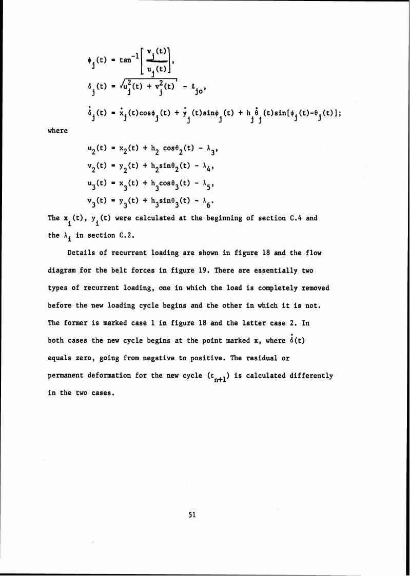
where

u2 (t) = x2(t) + h2 cose2(t) - A3,

v2(t) = y2(t) + h2sine2(t) - A4, u3(t) x3(t) + h cose3(t) - A 5 ,

3

v3(t) = y3(t) + h3sine3(t) - A6.

The x (t) (t) were calculated at the beginning of section C.4 and i ' Yi

the Xi in section C . 2 .

Details of recurrent loading are shown in figure 18 and the flow

diagram for the belt forces in figure 19. There are essentially two

types of recurrent loading, one in which the load is completely removed

before the new loading cycle begins and the other in which it is not,

The former is marked case 1 in figure 18 and the latter case 2, In *

both cases the new cycle begins at the point marked x, where b(t)

equals zero, going from negative to positive. The residual or

permanent deformation for the new cycle (c ) is calculated differently ntl

in the two cases.

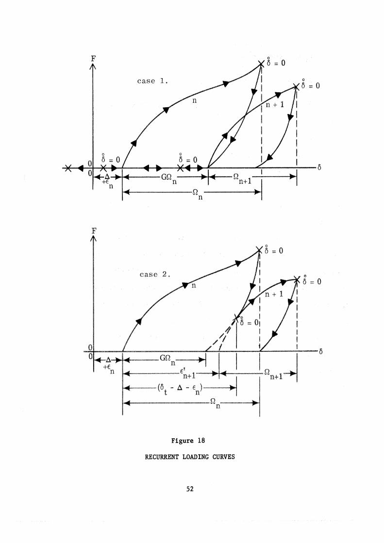
Figure 18

RECURRENT LOADING CURVES

Note: if j = 1, F ( t ) is for b abclomen otherwise for chest

Compute $.(t)

r - L - 4

Figure 19

BELT FORCE FLOW DIAGRAM

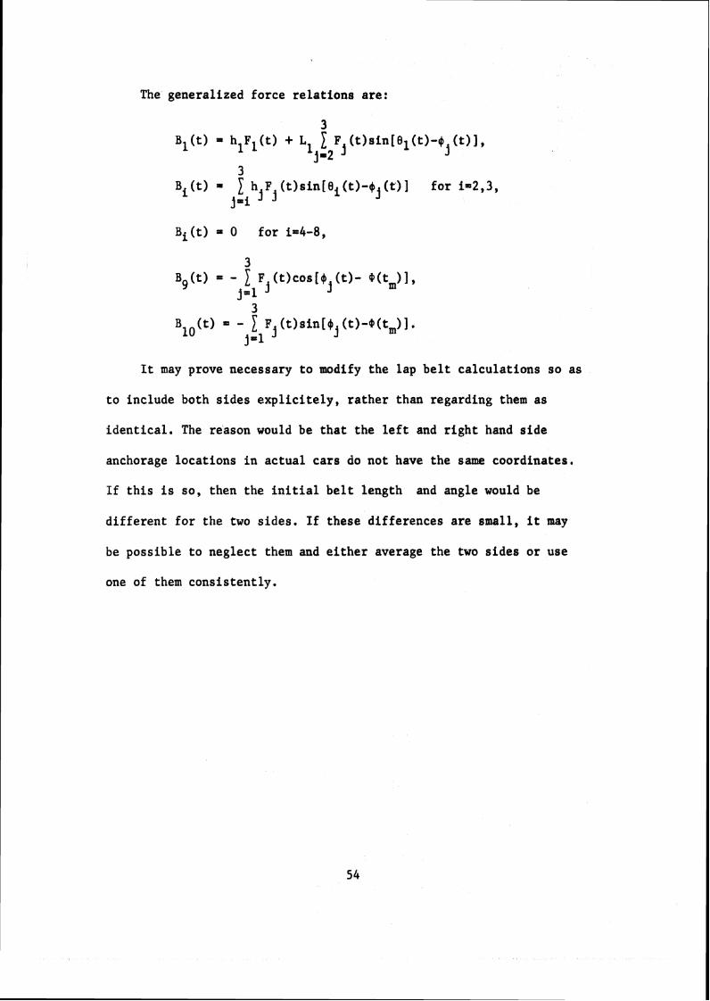
The generalized force relations are:

3 ~ ~ ( t ) = 1 h F (t)sin[8i(t)-$j(t)l for i=2,3,

jPi j j

Bi (t) = 0 for i=4-8,

It may prove necessary to modify the lap belt calculations so as

to include both sides explicitely, rather than regarding them as

identical. The reason would be that the left and right hand side

anchorage locations in actual cars do not have the same coordinates.

If this is so, then the initial belt length and angle would be

different for the two sides. If these differences are small, it may

be possible to neglect them and either average the two sides or use

one of them consistently.

SECTION C . 4 . f

CONTACT FORCES

The contact surfaces considered are both sides of the head rest

and seat back, the roof, windshield, sun visor, upper and lower

instrument panels, floor and toeboard, and steering wheel rim and

column. All of these except the head rest, sun visor, and steering

wheel are assumed to be rigidly fixed relative to the interior of

the vehicle. It is further assumed that the characteristics of the

motion and material of the nonrigid surfaces can be lumped, with the

exception of the column which may be padded. In this latter case,

it is assumed that the column does not move until its padding (if

any) has bottomed out. These assumptions simplify the calculations

a great deal and are sufficiently realistic.

In this present simulation, the nonrigid contact surfaces are

characterized by load-deflection relations rather than by explicit

differential equations. The latter is a better and more accurate

representation, but requires that the number of degrees of freedom

of the system be raised by approximately six, since the rim and

column would need at Peast two degrees of freedom each and the head

rest and sun visor one. This will be done in phase three.

Figure 20 shows the overall contact force flow diagram; its

more complicated parts are defined in figures 22 to 24 and in

tables 7 to 11.

The body reference point coordinates and their velocities are

calculated from the following equations, referred to in figure 20 as

Calculate Calculate In x p ) , y;(t) Specifyk

i= 1 Ti(t), gik(t), bik(t) g;(t), ;;(t)

r from Table 7 f rom Eqn's f . 2,

f rom Eqns. f . 1 4 Fig. 21, and Table 8 -

to Fig. 22.

Time T = t v Out

f rom Table 10

l

I L

Calculate Pi(t) Calculate Pi(t)

f rom Fig. 23 f rom Fig. 24

I I + Calculate vT f rom Eqn. f . 3

Calculate

Figure 20

CONTACT FORCE FLOW DIAGRAM

equations f . 1 .

i=4 : x&(t) x ~ ( ~ ) + P ~ c o s ~ ~ ( ~ ) ;i(t)=i4(t)-~4il (t)sine4 (t)

yi(t) = y4(t)+p4sine4(t) j ~ ( t ) = j 4 ( t ) + p 4 d 4 ( t ) ~ ~ ~ ~ 4 ( t )

i=8 : x' (t)=x (t)+L c0s0~(t) 8 7 8 7 8 8

$(t)=; (t)-L 6 (t)sine8 (t)

y;(t)=~~(t)+L~sin~~(t) i;l(t)j7(t)tL8~8(t)cose8(t)

is10 : x' (t)=x (t)tL cose (t) 10 6 6 6 10 6 6 6 6

;I (t)4 (t)-~ B (t)sine (t)

y ' (t)ay (t)tL6sine6(t) 10 6 6 6 6

;;o(t)=;6(t)t~ B (t)cose (t)

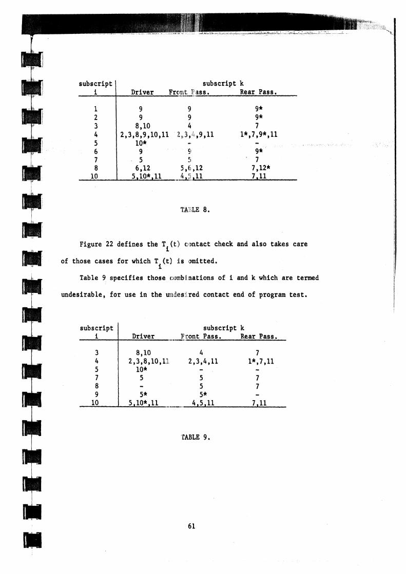
Table 7 shows what surfaces can be contacted by which body

segments for the three occupant positions.

I subscript k

Body Subscript Segment i

where l* indicates the back of the front-seat head rest, 5* the lower

Driver Front-Seat Rear-Seat Passenger Passenger

hip 1 back 2 chest 3 head 4 shoulder 5 elbow 6 knee 7 foot 8 shin 9 hand 10

edge of the lower panel,6* the sloping section of the rear-seat floor,

9 9 9 * 9 9 9*

8,lO 4 7 1,2,3,8,9,10,11 1,2,3,4,9,11 1,7,9*,11,1*

10 - - 9 9 9* 5 5 7

6,12 5,6,12 6*,7,12* 5* 5 * -

5,10*,11 4,5,11 7,11

9* the rear-seat back, lo* the side rim of the steering wheel, and

12* the rear-seat floor.

TABLE 7.

Equations f .2 for T (t), bik(t) and dik(t), as derived from i

the various geometries shown in figure 21, are as follows:

iik(t) ' ;'(t)co~$~ i - ;;(t)sin$k, Ti(t) = [xt'-x' (t) 1~0s) + [y"-y' (t)]sinqk,

k i k k i

for the (i ,k) sets of table 8, with Ti(t) omitted for k=11,12. Speci 1 .

relations needed here are: xl'=x"-D cos) , y"=yl'-D sin$2, 1 ) , .. \ 5 ' , 4 2 2 2 4 2 2 10 8

It UY" my"-D sin$6; Y1l 2' '12=009 YE^ 6 6

for i=4, k=1 and where

bik(t) = r - [xu-D5cos) -xl (t) ]sin[0 (t)-ao] 7 5 5 7 8

+ [y"-D sin) -yl (t)]cos[B8(t)-aO], 5 5 5 7

Ti(t) = [XI'-D COS) -xl (t)]~os[0~(t)-a y - i n y t 1 8 t - f 5 5 5 7 0 5 5 5 7 0 9

for i=9, k=5*, where a. was defined and calculated in section C . 2 .

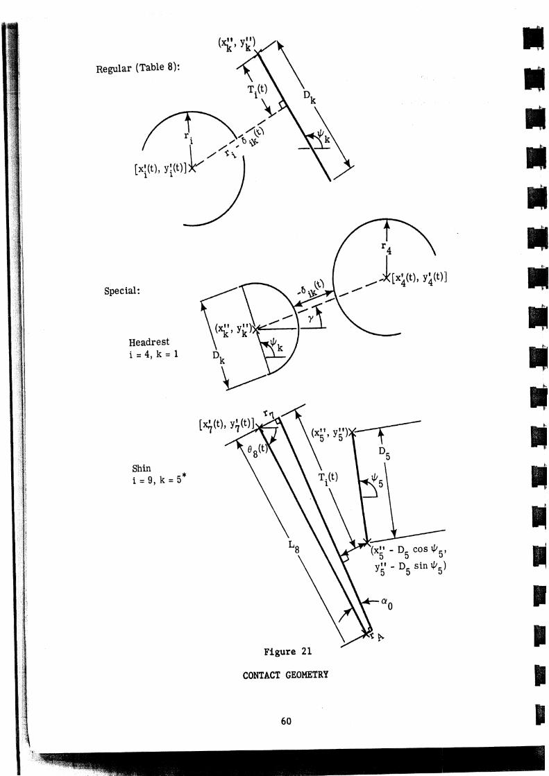
Special:

Headrest i = 4 , k =

Shin i = g , k = 5 *

Figure 21

CONTACT GEOMETRY

subscript subscript k Rear Pass.

'I'A LE 8.

Figure 22 defines the T (l;':~ c : )ntact check and also takes care i

of those cases for which T ( t ) :is ~mitted. i

Table 9 specifies those c.r,larbl nations of i and k which are termed

undesirable, for use i n the UII . ! ,~?,~: red contact end of program tes t .

subscript subscript k 1; cont Pass. Rear Pass.

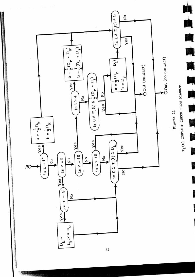
Table 10 defines, both numerically and descriptively, the

composition of any particular contact surface, whether a single

material, a padded surface, or a nonrigid surface.

subscripts Contact Surface k I 8 Composition

I head rest 1 windshield 2 sun visor 3 upper panel 4 lower panel 5 toeboard 6 back of front seat 7 steering column 8 seat back 9 steering wheel rim 10 roof 11 floor 12

non-rigid motion

8 non-rigid motion 2 glass 9 non-rigid motion 3,6 padded metal 3,6 padded metal 4,s mat onfloor 1 seat material 3,10 padding plus non-rigid motion 1 seat material 7 non-rigid motion 3,6 paddedmetal 4,5 mat on floor

Body Segment i

abdomen 1 chest 3 face 4 shoulder 5

TABLE 10.

Table 11 shows the combinations of i and k for which contact

deflection is shared; i.e. deflection occurs both in the body and in

the surface.

. . . . *

b for

11 12 13 14

subscrlp t subscript K Driver Front Pass, Rear Pass.

4 8,lO 4 l*, 7 5 lo* - -

TABLE 11

63

E . ( t ) = Eiit - A t ) A E i ( t ) G b

Out

Figure 23

SHARED DEFLECTION CONTACT FORCE FLOW DIAGRAM

Figure 23 displays the flow diagram for this shared deflection

force, while figure 24 contains that for deflection in or of the

surface only. Figure 25 depicts a bi-material force-deflection curve.

Equations 2.3 define the tangential velocity of the body along

the contact surface, as follows:

v = xl (t)cos$ + ;! (t)sin$ + r 6 (t) for the Table 8 (i,k), l" 1 k 1 k i i

v T =;~(t)cosu-;i(t)sinv+r 4 6 4 (t) fori=4,k=l,

vT - $,(t)cos[e8(t)-ao] + ;;(t)sin[e8(t)-a o ] + 6 97 (t); 8 (t) for 1.9, k = e

Equations f .4 define the present horizontal and vertical contact

force components, relative to the interior of the vehicle, for each

contacting body segment in terms of the normal and tangential forces

and the angle of the contact surface with respect to the floor. The

program also allows for the case in which one body segment contacts

more than one surface at the same time, which is theoretically

possible but practically unlikely. Special relations needed in these

equations are: $11=1800, $12=00. The proper (i,k) sets from

Table 7 must be used.

P S (t) = P ( s i n + P' (t)co~$~ 1 1 k i

i=9: PS9 (t) = P (t)sin[ao-e8(t)] + Pi (t)cos [ao-e8(t)] 9

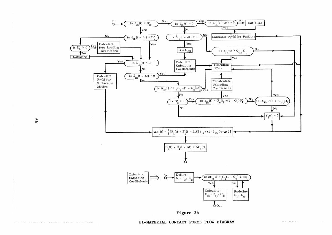
Parameters

- f L - Coefficients

Recalculate A L

Motion Coefficients

No T r

!I

1 aE. ( t ) = Z[Fi(t) + Fi(t - ~ t ) ] r 6 ~ ~ ( t ) - d ~ ~ ( t - ~ t ) l -

Figure 24

BI-MATERIAL CONTACT FORCE FLOW DIAGRAM

After all these contact force components have been calculated

for all the contacting body segments, the three main force-based

injury criteria can be evaluated. Figure 26 shows the flow diagram.

These are the tension dislocations of joints and compression and shear

fractures of bones. Table 5 in section C.l shows the correspondence

between the subscript i and its particular bone in each case. The

forces are calculated in equations f.5, f.6, and f.7 respectively.

Equations f ,5

FT1 = (F +PC1+PC +PC -F1-PC8-PC )sin8 S 2 4 s 9 1

+ (f-PS -PS -PS~-FI+PS +PS +PS )COS~ 1 2 s 7 8 9 1'

FT2 = (PC +PC -F )sin8 + (PSI-PS2-PS4-f)cos8 2 4 s 2 2

+ F cos (8 -) ) - F2cos (82-(2), 3 2 3

FT (PC -F -PC )sine3 + (PSI-f-PS7)cos8 3 4 s 1 3

+ F2cos ( O - 4 ) + F3~~~(83-43), 3 2

FT4 = (PC -F -PC -PC )sing4 + (PS1+PS2-f-PS )cos8

4 s 1 2 4 4

+ F cos ( 8 -( ) - F1cos (84-$1) - F3cos (84-43), 2 4 2

FT = (PC5+PC +PC -F -PC1-PC2-PC )sin0 - Flcos(e -( ) 5 6 10 s 4 5 5 1

+ (PSl+PS2+PS -f-PS -PS -PSI(-,) cos8 4 5 6 5

+ F2cos (05-(2) - F3cos (8 5 - 4 3 ) ,

FT6 (PC6+PC10-PC2-PC 5 ) sin8 6 + (PS 2 +PS5-PS6-PS 10 ) ~ 0 ~ 8 ~

FT7 = (PC7+PC8+PC 9 S S -F -F')~in8~ + ( P S 1 - £ - ~ ; - P S 7 - P S d ~ ~ ) c o s 0 8'

Calculate FTi i = l i s FTi > 0 from Eqns. f . 5

4 No I NO No Yes

i s i > 7 i = i + l 1 t

Print "TENSION DISLOCATION OF JOINT I = i AT TIME T = t"

Figure 26

FORCE-INJURY CRITERIA F L O W DIAGRAM

- + Calculate FSi is I FS. I k FSFi Yes From Eqns. f . 7 L

Print "SHEAR FRACTURE OFBONE I = i A T TIME T = t

No

Y i = i + l Yes

Equations f ,6

FC1 = (f-PS1+PS2+PS4)~os01 + (F s +PC1-PC2-PC )sine1 4

+ F c0s(0~-4~) - F3c0S(0 -$ 1, 2 1 3

FC2 = (f-PS1+PS +PS )cos02 + (F + P C ~ - P C ~ - P C ~ ) ~ ~ ~ ~ ~ 2 4 8

+ F ~ C O S (02-01) + F3c0s (02-$3),

FC3 = (I-PS1+PS )cos0 + (Fs+PC1-PC4)sin03 + Flcos (0 -0 ) 4 3 1 3

- F2c0s (83-42) 9

FC4 omitted,

Equations f .7

FS1 = F1'

FS2 = F2sin(02-$2),

FS3 = F3sin(03-03),

FS = P4, 4

FS5 = -PS sine - PCpcosO 2 3 3 '

FS6 = -PS 3 sine3 - PC3cos0 3 ' = F'COS~

FS7 s 7'

FS8 = P 9"

FS9 = P 7

Finally the contact generalized forces are calculated from

Equations f .8, as fol.lows:

Q3(t) - L [PS (t)~in0~(t)+PC~(t)cos8~(t)I - r2Pi(t) - r P' (t) 3 4 3 3

Q (t) = p i [PS4(t)sine4 (t)+PC4(t)cose4 (t) ] - r4Pi(t), 4

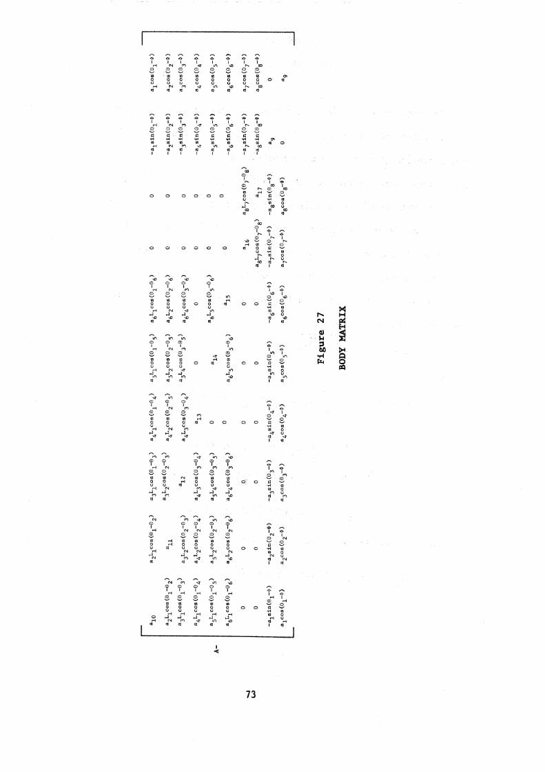
SECTION C . 5

ACCELERATIONS

In the present simulation, t he vehic le accelerat ions a r e read

from tab les . These include the horizontal and v e r t i c a l acce lera t ions

of the vehic le center of gravi ty and i t s p i t ch accelerat ion.

The accelerat ions of the generalized coordinates f o r the body

-f +- a r e found by invert ing the matrix equation Az = b and solving. The

-f vector b has already been computed i n Section C . 4 . The matrix A

is shown i n f i gu re 27, where t h e a were defined and computed in 1

Section C . 2 .

. . . . . . . . . . . . - . . . 8 8 8 e 0 ,e a a

I I 1 I I i N m u In 'm I r r ' m 0 g g 2 $ 2 % b'

m m m m m m m m m o o o o o o 0 8 0 m Ll L ) U U U U U 3 b u r n

rd r d m Z ? m U l t r d D O

e m

0 - I, t z- 0 r - I

\D - - m 8 0 b

m o a - U r i m l.m 0

$2 )

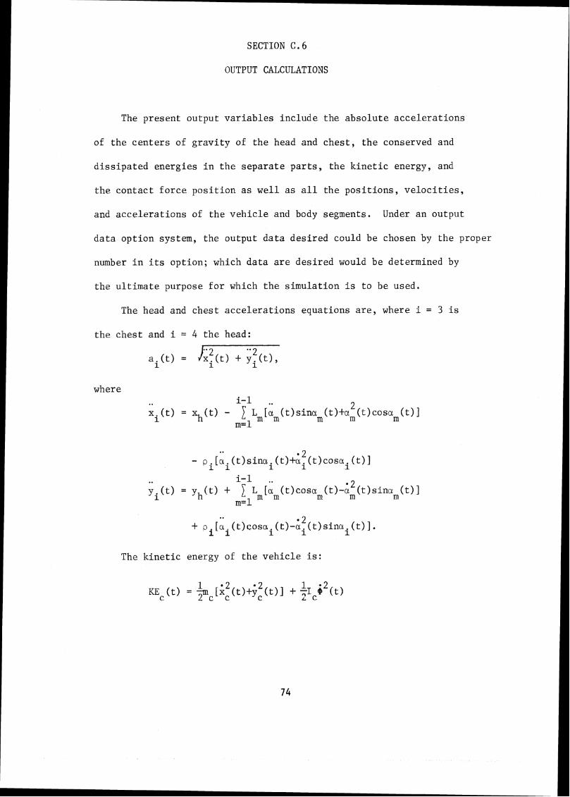
SECTION C.6

OUTPUT CALCULATIONS

The p r e s e n t ou tpu t v a r i a b l e s i n c l u d e t h e a b s o l u t e a c c e l e r a t i o n s

of t h e c e n t e r s of g r a v i t y of t h e head and c h e s t , t h e conserved and

d i s s i p a t e d e n e r g i e s i n t h e s e p a r a t e p a r t s , t h e k i n e t i c energy, and

t h e c o n t a c t f o r c e p o s i t i o n a s w e l l a s a l l t h e p o s i t i o n s , v e l o c i t i e s ,

and a c c e l e r a t i o n s of t h e v e h i c l e and body segments. Under a n ou tpu t

d a t a o p t i o n sys tem, t h e o u t p u t d a t a d e s i r e d could be chosen by t h e proper

number i n i ts o p t i o n ; which d a t a a r e d e s i r e d would be determined by

t h e u l t i m a t e purpose f o r which t h e s i m u l a t i o n is t o be used.

The head and c h e s t a c c e l e r a t i o n s equa t ions a r e , where i = 3 i s

t h e c h e s t and i = 4 t h e head:

where

The k i n e t i c energy of t h e v e h i c l e i s :

The conserved and d i s s i p a t e d e n e r g i e s i n t h e s e a t a r e due t o

i t s s p r i n g s , l i n e a r and n o n l i n e a r , and t o t h e damper and f r i c t i o n ;

i . e . :

1 . D E W = D E ( ~ - A ~ ) + 5 { ~ s ~ Y l ( t ) + ; l ( t - ~ t ) I [ ~ ~ ( t ) - ~ ~ ( t - ~ t ) I

+ [f ( t )+f (t-At) ] [xl ( t ) -xl (t-At) ] 1.

I n t h e j o i n t s , t h e conserved energy is due t o t h e e l a s t i c i t y

and t h e d i s s i p a t e d t o f r i c t i o n and r e s t r a i n t s ; t h u s f o r each j o i n t

( i = 1 t o 7 ) :

2 C E ~ ( ~ ) = K ~ [ O ~ ( ~ ) - O ~ ( ~ ) + O ~ ~ - O ~ ~ I ,

(0 otherwise .

The g r a v i t a t i o n a l energy i s a l l conserved; f o r each body segment

where

y f g ( t ) = y i ( t ) + pisinOi(t) f o r i - 1 t o 6, 1

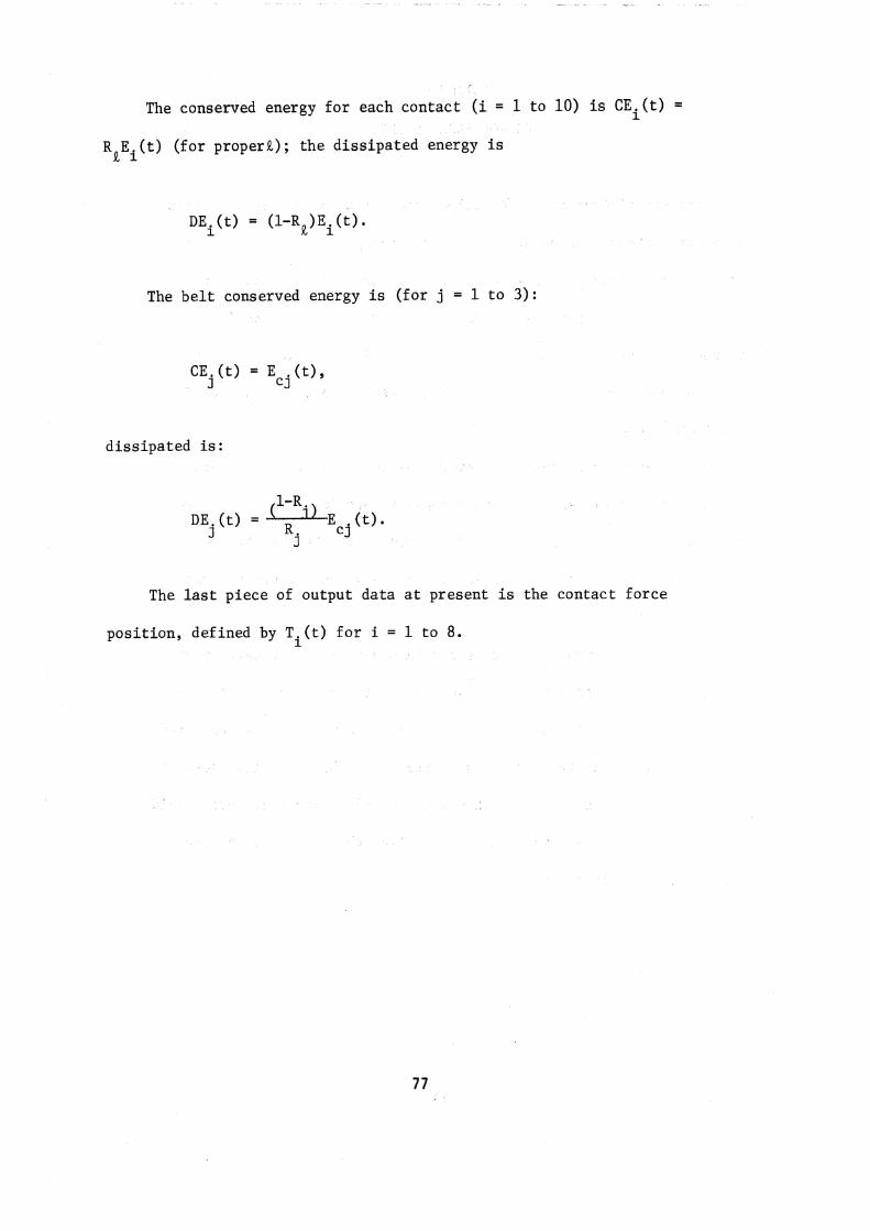
The conserved energy f o r each c o n t a c t ( i = 1 t o 10) is CEi(t) =

R E . ( t ) ( f o r p roper&) ; t h e d i s s i p a t e d energy i s Q 1

The b e l t conserved energy i s ( f o r j = 1 t o 3 ) :

d i s s i p a t e d is:

E ( t ) . DEj(t) = j

c j

The l a s t p i e c e of ou tpu t d a t a a t p resen t i s t h e c o n t a c t f o r c e

p o s i t i o n , de f ined by T i ( t ) f o r i = 1 t o 8.

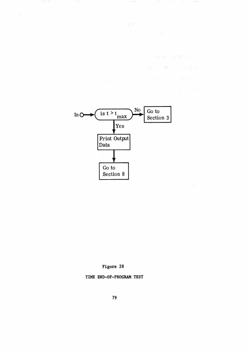
SECTION C, 7

END-OF-PROGRAM-TEST

The end-of-program option allows the selection of several tests.

At present these choices are time only, time plus undesired contact,

and time plus injury, Thus the time duration of the program run is

always one of the criteria for the end-of-program test, and in fact

is the only one contained in this section. It is shown in figure 28,

The undesired contact test is contained in Section C.4.f as Table

g and in figure 20.

The injury test occurs in several places; that for joint dis-

location due to excessive relative angle in Section C.4.c in figure

10 and the others in Section C. 4. f, figure 20 and figure 26 *

Another criterion that could be used as an end-of-program test

is the cessation of body motion.

Which end-of-program test is chosen would depend in large part

on what the simulation is being used for. If the purpose is to in-

vestigate or test various restraint systems, then time plus undesired

contact would probably be the best criterion to use. If the interior

vehicle design is the object, then the time plus injury criteria would

be of value. If the purpose is just to find the motion, then time

alone will be sufficient.

In Section 3 I I Print Output

I D a t a , I Section 8 w

Figure 28

TIME END-OF-PROGRAM TEST

SECTION 8

MODIFICATIONS

It would be extremely usefu l f o r the program i t s e l f t o be ab le

t o eva lua te i t s own r e s u l t s , change c e r t a i n input parameters o r da t a ,

and then i n i t i a t e a new run. The c r i t e r i a f o r such evaluat ions and

changes would depend on the u l t imate use of the program, a s would the

se l ec t ion of parameters t o be var ied .

For example, i f the program were being used t o eva lua te r e s t r a i n t

systems, then the n a t u r a l parameters t o be var ied would be those of

the b e l t mater ia l and t h e i r anchorage loca t ions , The evaluat ion c r i t e r i a

could be the use of the undesired contact end-of-program t e s t , the

i n ju ry c r i t e r i a f o r the to r so and neck, and/or la rge forces i n the b e l t s

themselves.

The method of changing the parameters could be e i t h e r systematic

o r random, and they could be changed e i t h e r s ing ly o r a l l a t the

same time.

SECTION D

A SIMPLE ANALOG TO COLLISION BETWEEN AUTO OCCUPANTS

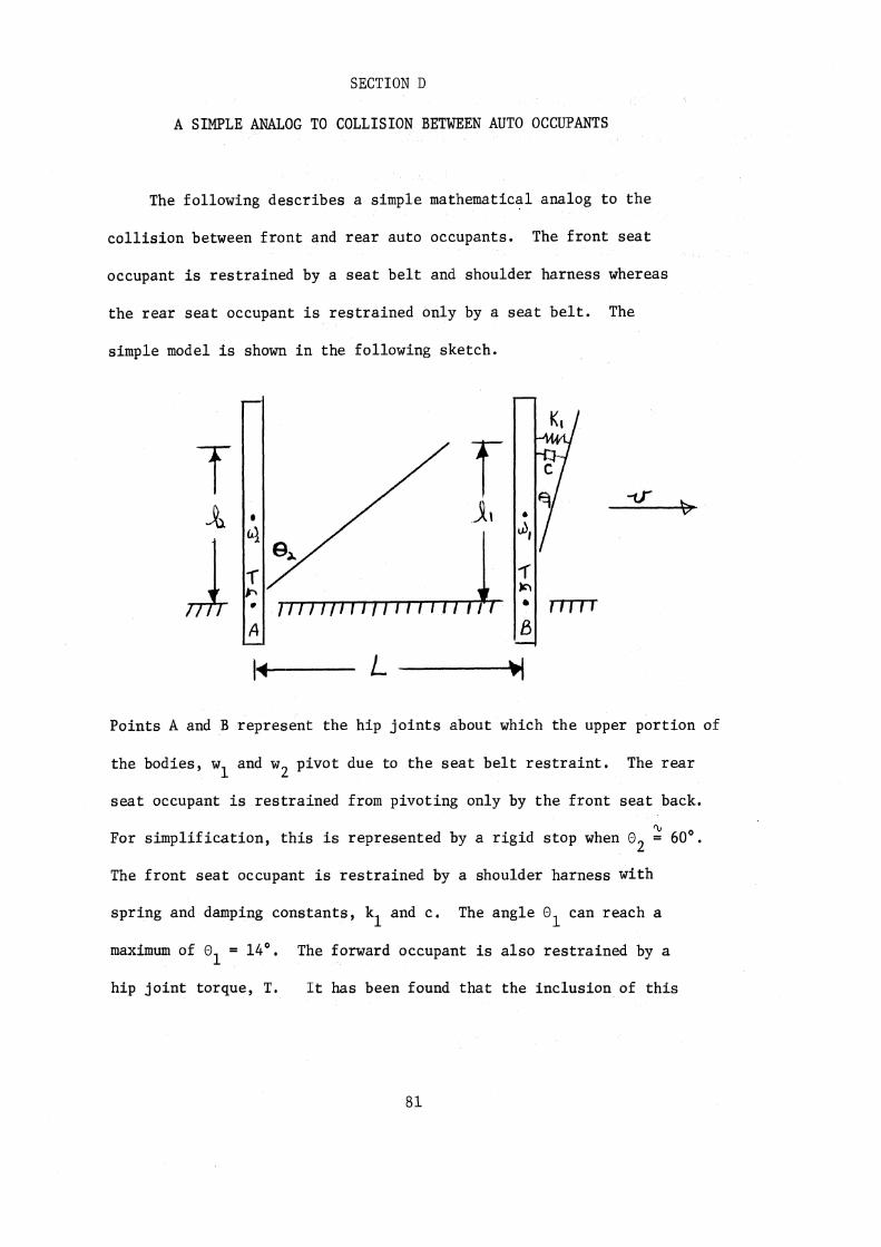
The fol lowing d e s c r i b e s a s imple mathematical analog t o t h e

c o l l i s i o n between f r o n t and r e a r au to occupants. The f r o n t s e a t

occupant i s r e s t r a i n e d by a s e a t b e l t and shoulder harness whereas

t h e r e a r s e a t occuparit i s r e s t r a i n e d only by a s e a t b e l t . The

simple model i s shown i n the fol lowing sketch.

P o i n t s A and B r e p r e s e n t t h e h i p j o i n t s about which t h e upper p o r t i o n o:E

t h e bodies , w and w2 p ivo t due t o t h e s e a t b e l t r e s t r a i n t . The r e a r 1

s e a t occupant i s r e s t r a i n e d from p ivo t ing only by t h e f r o n t s e a t back.

rl, For s i m p l i f i c a t i o n , t h i s is represen ted by a r i g i d s t o p when O = 60'. 2

The f r o n t s e a t occupant i s r e s t r a i n e d by a shoulder harness wi th

s p r i n g and damping c o n s t a n t s , kl and c . The ang le O can reach a 1

maximum of O = 14'. The forward occupant i s a l s o r e s t r a i n e d by a 1

h i p j o i n t torque, T. It has been found t h a t t h e i n c l u s i o n of t h i s

r e s t r a i n t on t h e r e a r occupant i n c r e a s e s t h e amount of t ime between

i n i t i a l impact and f i n a l s t o p by abou t 8%. The i n i t i a l forward

v e l o c i t y i s v . The o b j e c t i v e of t h e fo l lowing i s t o show a s imp le

ana log t o t h e d i f f e r e n c e between i n t e r o c c u p a n t motion i n t h e c a s e s

where t h e f r o n t shou lde r h a r n e s s i s a n undamped s p r i n g and where i t

i s c r i t i c a l l y damped.

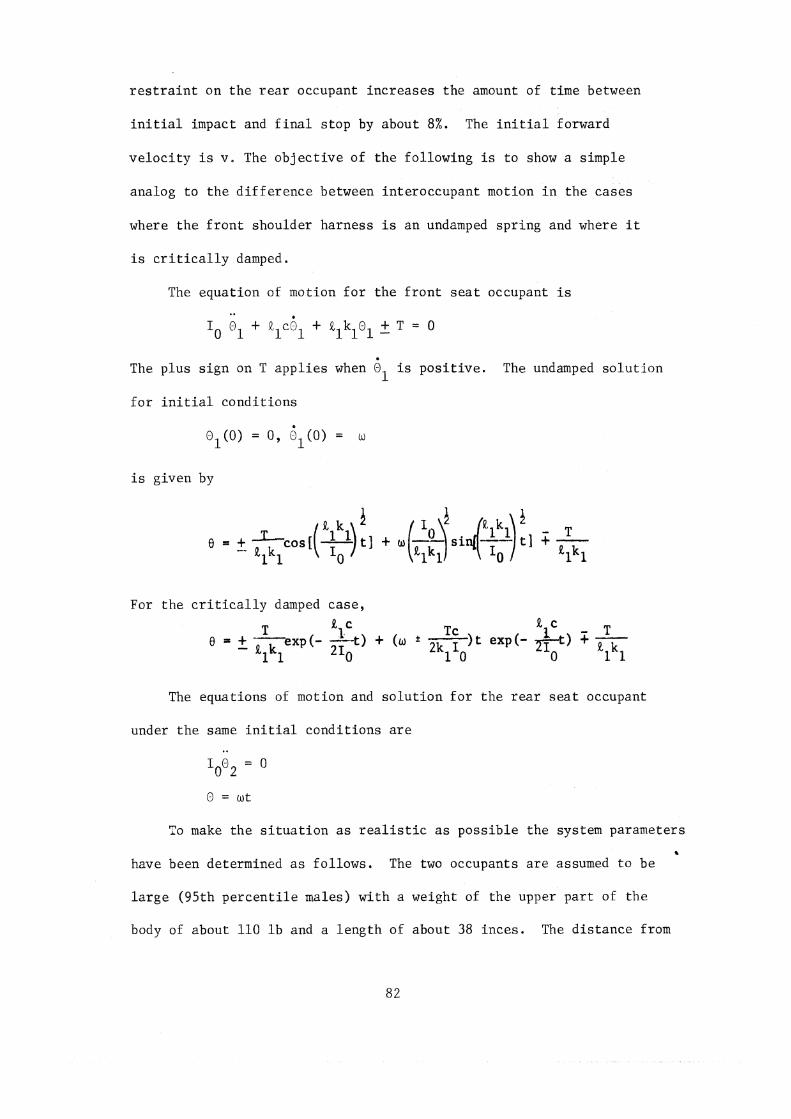
The e q u a t i o n of motion f o r t h e f r o n t s e a t occupant i s

. The p l u s s i g n on T a p p l i e s when O i s p o s i t i v e . The undamped s o l u t i o n

1

f o r i n i t i a l c o n d i t i o n s

i s g iven by

For t h e c r i t i c a l l y damped c a s e ,

The equa t ions of motion and s o l u t i o n f o r t h e r e a r s e a t occupant

under t h e same i n i t i a l c o n d i t i o n s a r e

To make t h e s i t u a t i o n a s r e a l i s t i c as p o s s i b l e t h e system pa rame te r s

have been de termined a s f o l l o w s . The two occupants a r e assumed t o be

l a r g e (95 th p e r c e n t i l e males) w i t h a weight of t h e upper p a r t of t h e

body of about 110 l b and a l e n g t h of abou t 38 i n c e s . The d i s t a n c e from

t h e p ivo t p o i n t t o t h e c e n t e r of g r a v i t y was taken t o be 17 inches 9

y i e l d i n g I = 117 lb-in-secL. 0

The i n i t i a l angu la r v e l o c i t y was found by no t ing t h a t i n i t i a l l y each

body possessed a given l i n e a r momentum which had a moment of momentum

about t h e p ivo t po in t of

mvp = I o 0

For a 20-mph c o l l i s i o n , w = 14.7 r a d l s e c .

By t r i a l and e r r o r i t was found t h a t a s p r i n g cons tan t K = 25,000

l b / i n . stopped motion of t h e forward occupant i n 0.026 s e c f o r t h e

'I, undamped c a s e a t about 0 = 14". Using t h e previously determined 1

% parameters t h e damping c o e f f i c i e n t was found t o be c = 830 lb-sec.

The motion i n t h e undamped case proceded a s fol lows. A t t = 0.026

s e c , t h e forward t h r u s t of t h e f r o n t occupant had been a r r e s t e d by t h e

'I, 'I, shoulder harness a t O = 14". The r e a r occupant had pivoted t o O = 22" 1 2

i n t h i s time, The complete time h i s t o r y is:

t ime(sec) O (approx) 1 O 2 (approx)

The simple ske tch below shows t h a t con tac t must have occurred between

t h e two occupants between t = 0.050 and t = 0.075 i f a t y p i c a l s e a t

s e p a r a t i o n (L = 34 inches) i s used.

Dot ted l i n e s r e p r e s e n t t h e f i n a l p o s i t i o n s .

For t h e damped c a s e numer ica l c a l c u l a t i o n s show t h a t t h e s o l u t i o n is

dominated by t h e term

Rlc t O = w t exp --

210

Th i s term i s never n e g a t i v e , and t h u s t h e sp r ingback caus ing i n t e r o c c u p a n t

c o l l i s i o n us ing t h i s model i s imposs ib l e . By t h e t ime t = 0.125, O lo I

The major o b j e c t i v e of t h e s imp le s tudy h a s been accomplished. The

model h a s shown t h a t c o l l i s i o n between t h e two masses may o r may no t

occur depending on system damping. Other parameters i n t h e model

b e s i d e s damping w i l l a l s o p l a y a major r o l e , These a r e s i z e of masses,

p i v o t p o i n t l o c a t i o n , r a t e of speed , geometry of r e s t r a i n t s , p i v o t

p o i n t r e s t r a i n t f r i c t i o n , e t c . , a l l of which a r e i n t h e model and can

be v a r i e d . These pa rame te r s can be cons ide red analogous t o s i z e of

occupant (not a l l d r i v e r s and occupants a r e 95 th p e r c e n t i l e male

dummies), s e a t l o c a t i o n , r a t e of speed , h a r n e s s and s e a t b e l t geometry,

j o i n t f r i c t i o n , and s e a t d e s i g n and p r o p e r t i e s .

REFERENCES

1. McHenry, R.R.: Analysis of the Dynamics of Automotive Passenger Restraint Systems, CAL No. VJ-1823-R1, May 31, 1963.

2. Naab, K.N.: A Computer Simulation of the Crash Victim- Comparison of the Results Obtained with Different Integration Routines, Time Increment Sizes, and Joint Friction Lags, CAL No, VJ-1823-R18, March 1966,

3. McHenry, R.R. and K.N. Naab: Computer Simulation of the Automobile Crash Victim in a Frontal Collision -- A Validation Study. CAL No. YB-2126-V-1, July 1966.

4, Smith, J.W.: Observations on the Postural Mechanism of the Human Knee Joint, Journal of Anatomy V. 90 pt ,2, p ,236-261,

Acknowledgments are due to: Mark Berg for the

list of parameters and basic variables and for the rigid-

beam seat representation details, Prof. Kurt Binder for

Figure 2, Dr. Verne Roberts for ideas and suggestions,

Robert Bennett, Jr. for the computer programming, and

Marcia Mascarello for calulations.