1

BEAUTY, STATURE AND THE LABOUR MARKET:

A BRITISH COHORT STUDY.

Barry Harper

London Guildhall University

8 June 1999

ABSTRACT

The influence of physical appearance in the labour market is examined using longitudinal cohort data

covering 11,407 individuals born in Britain in 1958. Results show that physical appearance has a

substantial effect on earnings and employment patterns for both men and women. Irrespective of

gender, those who are assessed as unattractive or short, experience a significant earnings penalty. Tall

men receive a pay premium while obese women experience a pay penalty. The bulk of the pay

differential for appearance arises from employer discrimination, although we find evidence for

productivity differences among occupations. The impact of physical appearance is also evident in the

marriage market. Among women, those who are tall or obese are less likely to be married; while

among men, lower marriage rates are found for those who are short or unattractive.

JEL CLASSIFICATION NUMBERS: J7, J12, J15, J31.

KEYWORDS: Earnings, human capital, physical appearance, discrimination.

WORD COUNT: 4,367 (excluding references and tables).

ADDRESS FOR CORRESPONDENCE: Barry Harper, London Guildhall University, Department

of Economics, 84 Moorgate, London EC2M 6SQ, U.K. Fax ( +0171) 320 1498.

EMAIL: harper@lgu.ac.uk.

2

BEAUTY, STATURE AND THE LABOUR MARKET:

A BRITISH COHORT STUDY1

Barry Harper

Those who are well-endowed with desirable physical attributes are often thought to obtain significant

economic and social advantages over the not-so-well-endowed. A small but growing body of research,

almost exclusively from the USA, suggests that physical appearance, measured by attractiveness,

stature and body mass, has significant effects on the success of male and female workers in the labour

market. Wages have been found to be positively associated with attractiveness (Hamermesh and

Biddle, 1994; 1998) and height (Loh, 1993), and negatively related to obesity (Sargent and

Blanchflower, 1994; Averett and Korenman, 1996). Using longitudinal data drawn from the National

Child Development Study (NCDS)2 we examine the effect of physical appearance on hourly earnings,

employment patterns, and family income in Britain.

The paper makes the following contributions to the study of the effects of physical appearance

on the labour market. First, we examine the effect of being assessed as attractive or unattractive on

earnings for a British sample. All previous economic research has examined solely US data. Second, to

distinguish between pure employer discrimination and productivity effects, which include customer

discrimination, we assess whether the rewards for appearance vary by occupation. As a further test, we

1Earlier versions of this paper have benefited from comments by the editors, Jerry Coakley, Roderick Floud, George

Hadjimatheou, Gerry Kennally, Andrew Oswald and an anonymous referee. Mohammad Haq provided valuable research

assistance. We are grateful to Pierella Paci who provided earnings data and work history variables derived from NCDS

data. The author is responsible for any remaining errors.

3

examine evidence for hiring bias and occupational sorting arising from physical appearance. Third, we

update the work of Sargent and Blanchflower (1994) on the effects of height and obesity on earnings

in Britain. Finally, we examine the effect of physical appearance on household labour income via the

marriage market.

The paper is organised as follows. A simple human capital model of the effect of physical

appearance on hourly earnings is discussed in Section I. Section II examines unadjusted data regarding

physical appearance and economic attainment in the NCDS. Estimation results are presented in

Sections III-IV, and Section V contains a summary and conclusions.

I. THE MODEL

Physical appearance may affect labour market success for a number of reasons. First, worker

productivity may be affected directly by physical appearance. For example, Sorensen and Sonne-Holm

(1985) find that, controlling for social origin and intelligence test scores, obese individuals undertake

fewer years of schooling. Second, physical appearance may affect a worker’s productivity in a specific

occupation. This may arise either from physical productivity effects or from customer discrimination

(Becker, 1957). Third, as a result of pure employer discrimination, employers prefer individuals with

certain physical characteristics which are unrelated to their productivity. These preferences translate

into fewer job opportunities and lower pay for the less preferred group3.

2 The NCDS is a continuing longitudinal survey of individuals living in Britain who were born in the week 3-9 March 1958.

The most recent sweep in 1991 surveyed 11,407 individuals when aged 33.3Also, employers may erroneously ascribe personal qualities to individuals solely on the basis of their physical appearance.

Research by social psychologists, for example, suggests that greater height among men is positively related to perceived

social status which may, as a consequence, result in tall men being treated preferentially (Martel and Biller, 1987). We do

4

One approach to capture the effect of appearance on earnings is to estimate a standard earnings

equation

ln( )w X OCCi i i i i= + + + +α α α α λ ε0 1 2 3 (1)

where wi is the hourly wage of individual i, Xi represents a vector of productivity-enhancing

attributes, OCCi is the individual’s current occupation, λi is a vector of physical appearance

characteristics, and εi is a random error term. To examine any differential effects of appearance across

occupations, appearance/occupation interaction terms may also be included. The earnings equation

becomes

ln( )w X OCC OCCi i i i i i i= + + + + +β β β β λ β λ ε0 1 2 3 4 (2)

where β3 may be interpreted as the return to appearance regardless of occupation and β4 the differential

return to appearance which is occupation-specific.

The existence of pure employer discrimination would imply that β3 ≠0 and β4 = 0. Under these

restrictions the rewards to physical appearance will be independent of occupational status. As an

alternative test for employer discrimination we examine whether physical appearance affects an

individual’s probability of unemployment, which would be consistent with employer hiring bias.

Conversely, evidence for productivity differences obtains where β4 ≠0 and β3 = 0. As an additional test

we examine evidence for occupational sorting arising from physical appearance. Individuals are

expected to sort into occupations that reward a particular attribute and away from occupations where

penalties exist.

II. THE DATA

not examine this explanation in the paper. For a review of the literature on the psychological, social and economic effects of

5

The NCDS is a continuing longitudinal survey of individuals living in Britain who were born in the

week 3-9 March 1958. In the original 1958 survey 17,733 individuals were in the target sample. There

have been five subsequent sweeps of the original study, when members were aged 7, 11, 16, 23 and

33, by which time the achieved sample had fallen to 11,407. Of the 11,407 cases in the 1991 sweep of

the NCDS, 5,606 are male. The data cover an individual’s family background and his or her social,

educational and physical development. Mean values of selected variables for male and female

employees are presented, respectively, in Tables 1 and 2.

Each sweep of the NCDS contains information on the respondent’s height and weight.

Information on attractiveness is only available, however, for the respondent at age 7 and age 11. In

each of these sweeps the respondent’s teacher was asked to complete a questionnaire in an attempt to

acquire a picture of the child’s behaviour and character. Questions covered the respondent’s attitude

towards the teacher, school work, games and play. Teachers were also asked to assess the respondent’s

physical appearance in terms of the following categories: attractive/ not so attractive as most/ looks

very underfed/ has some abnormal feature/ nothing noticeable4.

Teachers’ assessments of the attractiveness of respondents at age 7 and age 11 are reported in

Table 3. Teachers placed most respondents in the attractive or average category with the proportion in

the former category decreasing between age 7 and age 11. One obvious concern is that teachers may

differ in what they consider to be attractive or unattractive. This measurement error will lower the

efficiency of our estimates. Evidence from previous studies suggests, however, that assessments of

physical appearance see also Hatfield and Sprecher (1986) and Jackson et al. (1995).4The variable abnormal feature was always insignificant in our estimated equations in a previous version of the paper.

6

beauty by individuals are quite uniform, change slowly over time, and that women’s appearances

evoke stronger reactions, whether positive or negative, than men’s (see Hatfield and Sprecher, 1986).

In Table 3 it would appear that the ratings of attractiveness are quite closely related at age 7 and age

11. Hence, 57.3% of young females were assessed as attractive at age 7, of whom, 64.8% were also

considered attractive at age 11. However, we attempt to reduce potential measurement error by

including information on attractiveness at both age 7 and age 11. We construct a simple measure

identifying those who were assessed as being attractive, or unattractive, at age 7 only, age 11 only, or

at both age 7 and age 115. Discussion on the interpretation of any link between appearance in

childhood, and earnings and employment in adulthood, is left until Section IV.

The height and weight of respondents was measured by interviewers at each sweep except at

age 23 when information on height and weight was self-reported6. Obesity is defined as an excess of

body fat. In this study we employ the Body Mass Index (BMI), defined as weight (in kilograms)

divided by the square of height (in meters), as an indirect measure of the individual’s fat composition7.

The average BMI values for males and females at age 23 and age 33, presented in Tables 1 and 2,

show a marked upward trend over the period 1981-91.

5Measurement error also appears to arise from the original coding of the data whereby missing and nothing noticeable are

not distinguished separately. All such cases are coded as nothing noticeable.6Height and weight data at age 33 are adjusted to exclude extreme values on the assumption that they reflect coding errors.

Height data are also adjusted where major discrepancies arise between age 23 and age 33. Details of excluded cases and

data adjustment are available from the author.7Measures of obesity most widely used are combinations of height, weight and skinfold thickness. All commonly used

measures are found to be highly correlated (Kannel, 1983).

7

We examine relative and absolute measures of obesity. The latter are based on medical

criteria8. To measure relative weight we construct indicator variables representing the location of the

respondent in the gender distribution of body mass, for a given age. Our findings suggest that relative

weight provides a better explanation of earnings than absolute measures of obesity. Social norms

regarding being considered as over-weight appear to be based, therefore, on relative weight criteria.

Unadjusted data, presented in Tables 1 and 2, indicate that those who are well-endowed with

desirable physical attributes obtain pay and employment advantages over the not-so-well-endowed.

These data reveal substantial unadjusted pay gaps between the attractive and unattractive of 19.5% for

males and 13.1% for females, and a pay gap between those who are tall and those who are short of

23.2% and 25.9% for, respectively, males and females. Obese males and females earn, respectively,

12.8% and 13.6% less than sample mean earnings for their gender. Also the likelihood of being

employed in a professional occupation increases for those who are attractive or tall, but decreases for

those who are unattractive, short or obese.

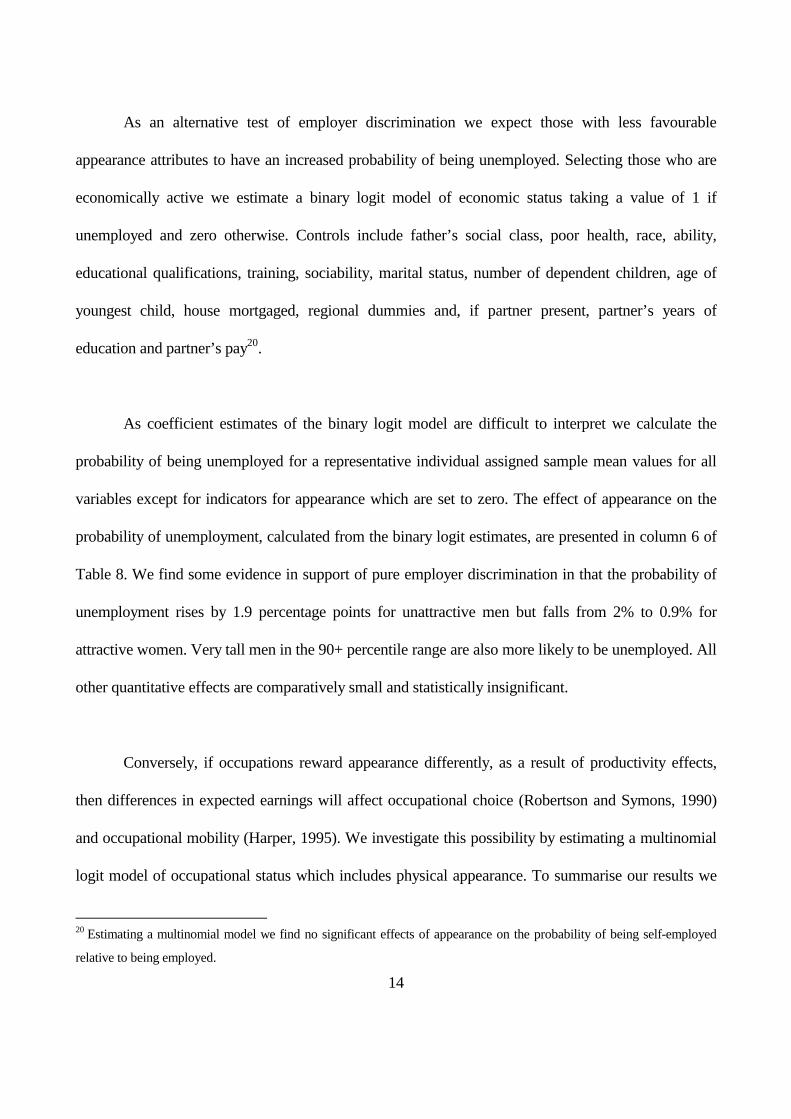
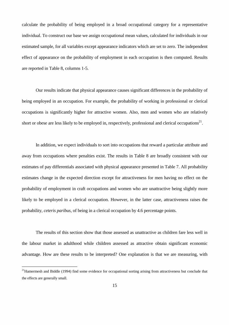
Even after controlling for occupation, significant pay differentials are still observed. Data

presented in Table 4 report, for example, an unadjusted pay gap between tall and short individuals

employed in professional occupations of 17.4% for males and 12.4% for females. In addition, data

presented in Table 5 indicate that appearance also affects the probability of employment. Those who

are unattractive or short have lower employment rates, typically arising from both lower activity rates

and higher unemployment rates.

8 This uses criteria, based on associated mortality risks, to identify weight categories The relevant BMI values for males

(females) are as follows; underweight<20 (<19), overweight 25-29 (24-29), and obese ≥30 (30).

8

III. APPEARANCE AND EARNINGS

Adopting the human capital model given in equation (1), we explain hourly earnings at age 33 as the

return to an individual’s endowment of productive attributes, investment in education and training, and

labour market experience. Our base sample is all respondents who are employees in 1991. Hence we

exclude those who are self-employed, unemployed or not economically active, giving a total of 4,160

males and 3,541 females9. In Table 6 we present results for earnings equations estimated separately for

men and women10. Body mass at age 23, rather than at age 33, is included, being potentially less

subject to endogeneity bias (Averett and Korenman, 1996).

In columns 1 and 4 of Table 6 regressions with controls for just health status, social class, and

race confirm our earlier observations from unadjusted data regarding the effects of physical appearance

on earnings11. Those who are attractive or tall have advantages over the unattractive, short or obese.

However, when we include controls for academic ability at age 11 and sociability at age 16 in columns

2 and 5, the effect of attractiveness on earnings becomes small and insignificant12. It would appear that

the assessment of attractiveness in our sample is not independent of the respondent’s academic ability

or personality. It may be that teachers were more likely to assess those with higher measured

9 We examine potential bias that may arise from employment selection. For panel attrition both Connolly et al. (1992) and

Harper and Haq (1997) find no evidence of estimation bias for males due to systematic data loss associated with panel drop-

outs or cases with ‘holes’ or missing information.10All estimates are obtained using LIMDEP 7.0. Details of controls used in the earnings equations are given in the notes for

the relevant tables. All results reported in the paper, but not presented in tables, are available from the author.11 Family background and health status are potential indirect routes by which appearance may affect earnings (Boldsen and

Mascie-Taylor, 1985; Kannel, 1983).12 Hatfield and Sprecher (1986) report that the one of the main observed differences between those assessed as attractive

and others is that they appear to be more sociable.

9

intelligence or those with a sociable disposition as attractive13; alternatively, attractiveness may be

correlated with an individual’s productivity14. Controlling for sociability is uncommon in economic

studies of appearance and earnings. Sociability therefore represents a potential source of bias in

research using interviewer assessments of attractiveness. Also, an advantage of using information up

to age 11 is that we reduce potential estimation bias arising from attractiveness, or unattractiveness,

and income being determined simultaneously or because interviewer-assessed standards of

attractiveness are spuriously correlated with the respondent’s earnings

Our preferred equations for the effect of physical appearance on the earnings of men and

women, which include an extensive set of controls, are reported in Table 6, columns 3 and 6. Controls

include, in addition to those reported for column 2, actual work experience, years of tenure with the

firm, and indicators for educational qualifications, training, trade union membership, part-time

employment, marital status, broad occupational category, firm size, industry and region of residence.

To increase sample size we include missing data indicators for both industry and region and recode

missed values of these variables to zero for all the relevant cases. Excluding cases where we have

missing data for industry and region leaves most coefficient estimates for appearance broadly

unchanged.

The results indicate asymmetry with respect to the effect of beauty on pay. It is those who are

assessed as unattractive, not attractive, who experience differential rewards in our sample. Men

assessed as unattractive at both age 7 and 11 incur a large and significant pay penalty of -14.9% while

13 See for example Felson et al. (1979).14 There is some evidence of a positive relation between both attractiveness and height with intelligence (Eisenberg et al.,

1984; Lynn, 1989; Jackson et al., 1995).

10

men assessed as unattractive at only age 11 experience a -4.0% pay disadvantage (Table 6, column 3).

A similar pattern of results is found for women. The effect of attractiveness remains insignificant

while women assessed as unattractive at both age 7 and 11 experience an earnings penalty of -10.9%.

The size of the pay penalty for unattractiveness is substantial and exceeds, in absolute value, the return

to education, compared to those with no qualifications, for all educational qualifications up to and

including A Level qualifications. Our estimates of the penalty of unattractiveness are larger than those

obtained by Hamermesh and Biddle (1994) for unattractive North American men and women of,

respectively, -9.1% and -5.4%. However, as in Hamermesh and Biddle (1994), we find that the penalty

for plainness exceeds the premium for attractiveness, and stronger effects for men than for women.

Results in Table 6 also update the estimates of Sargent and Blanchflower (1994) regarding the

effects of stature and obesity on earnings in Britain. People who are relatively short suffer an earnings

penalty. Men and women in the bottom 10% of the height distribution (less than, respectively, 1.685m

and 1.545m) 15experience, respectively, a -4.3% and -5.1% earnings penalty relative to individuals in

the excluded reference group representing the 20-79 percentile range. Relatively short men in the 10-

19 percentile range experience a smaller penalty of -3.8% while we find a significant pay premium of

+5.1% for short women in the same percentile range. Relatively tall men, but not the very tallest,

obtain a pay premium. Men in the 80-89 percentile range, who are around 6 feet tall (1.829m), earn

5.9% more than those of average height. The premium for the tallest men in the 90+ percentile range is

small and insignificant. We find no significant effects of being tall for women, which confirms social-

psychological evidence which emphasises the importance of height primarily among men. The results

also provide evidence of non-linearity in the relationship between height and earnings.

15Division into a percentile range is only approximate given the discrete nature of the measures of the respondent’s height

and weight.

11

Consistent with most other studies we find a significant pay penalty for obesity in women but

not men. Obese women who are in the top 10% of the weight distribution at age 23 experience a pay

penalty of -5.3% (Table 6, column 6). The penalty also extends to those women in the 80-89 percentile

range. The earnings differential of 6.4% for males identified by their teachers as having a sociable

disposition at age 16 represents a substantial premium. The effect of sociability of young females on

their earnings is smaller and insignificant.

We test for sample selection bias as our estimates are conditional on individuals being

employees16. The sample selection correction term for males, when included in the earnings equation,

is negative and significant, suggesting that, for male employees, unobserved variables influencing

employment selection are negatively related to male pay. The inclusion of the selection term results in

only marginal changes in the estimated coefficients, indicating that the bias arising from selection is

relatively small. We find no evidence of systematic selection for women in the NCDS cohort17.

Selection terms, which contain a substantial number of missing observations, are not included in our

final equations.

16The employee status selection term is derived from a multinomial logit selection model (Lee, 1983) for the outcomes of

inactive, unemployed/self-employed, and employee. Variables in the selection equation include controls for poor health,

ability, highest educational qualification obtained, house mortgaged, number of dependent children, age of youngest child,

partner’s earnings and region of residence.17Waldfogel (1995) reports similar findings for women in the NCDS.

12

IV. EMPLOYER DISCRIMINATION, PRODUCTIVITY AND OCCUPATIONAL SORTING

In this section we examine whether our results for physical appearance arise from pure employer

discrimination or from productivity differences which include customer discrimination. We estimate

equation (2) to assess whether differential rewards for appearance arise among occupations, which

would be consistent with productivity differences18. To reduce the number of appearance/occupation

interaction terms we include teacher’s assessment of the respondent’s attractiveness only at age 11. We

re-estimate our preferred equation, reported in Table 6, columns 3 and 6, following this substitution.

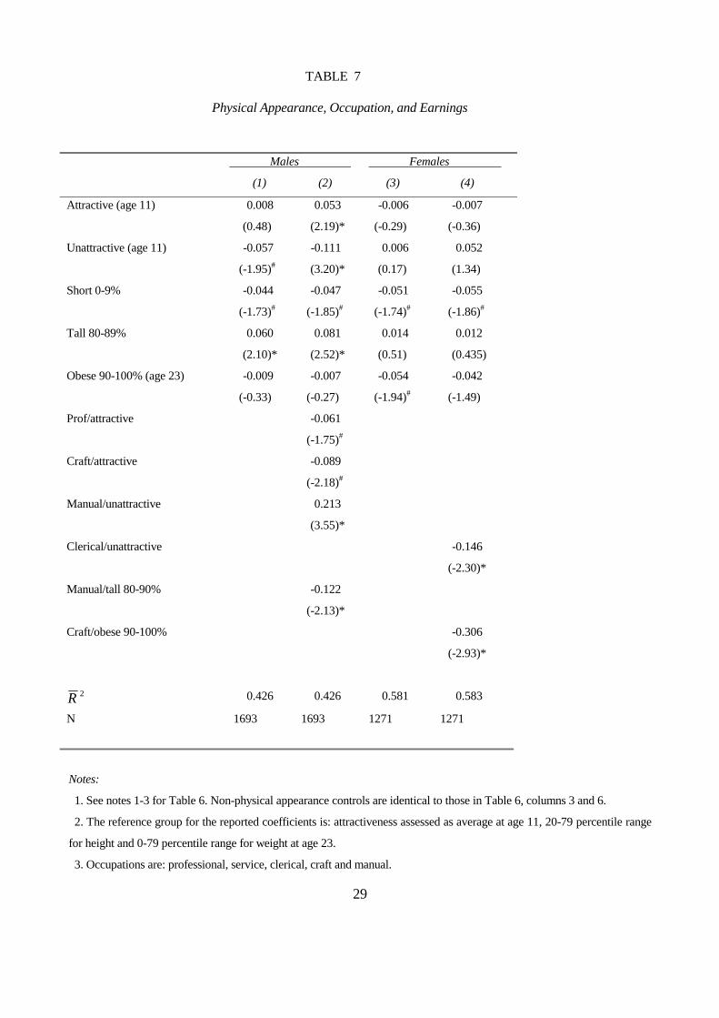
Results are presented in Table 7, columns 1 and 3. Excluding age 7 information reduces the estimated

penalty for unattractiveness (t-values in parentheses) for males and females to, respectively, -0.057

(1.95) and 0.006 (0.17).

We then include, in addition to our one digit occupational dummies, 20 interaction terms

between appearance and the respondent’s occupation19. The initial reference occupation being service.

Interaction terms with the lowest t-value are omitted sequentially to produce our preferred final

equations. The remaining significant interaction terms capture any differential effects of appearance on

earnings arising from appearance/occupation-specific productivity effects. Results for men and women

are presented, respectively, in Table 7, columns 2 and 4. The findings provide support for both pure

employer discrimination and productivity differences.

The estimated coefficient for unattractiveness, independent of occupational status, refers to the

effect of unattractiveness on earnings for individuals employed in the omitted occupational categories

18This result would also arise from non-uniform employer discrimination among occupations. We do not provide a testbetween the two approaches.19Of the possible appearance/occupation interactions we do not examine short 10-19%, tall 90-100%, or obese 80-89%.

13

for the unattractive/occupation interaction terms which are, in this case, professional, service and craft

occupations. This coefficient may be interpreted as the effect of pure employer discrimination. For

males the results do not alter, substantially, our previous conclusions. The penalty for unattractiveness

arising from employer discrimination is estimated to be -11.1%. This represents a large penalty for the

7.5% of male employees in our sample who were assessed as being unattractive. Our results also

provide evidence of employer discrimination against short males and in favour of tall males. Also

attractiveness becomes significant, with attractive males earning a premium of 5.3%.

While it appears that the bulk of the pay differential for appearance arises from employer

discrimination, we do find evidence for differential effects of appearance among occupations which is

consistent with productivity differences. For example, we find significant negative effects of

attractiveness on pay for men in professional and craft occupations which offset the general benefits of

attractiveness. Overall, the earnings differential for attractive males in professional occupations,

relative to individuals with average appearance, is just -0.8% (5.3% - 6.1%). Also, unattractiveness

appears to command a very large pay premium of +21% in manual occupations whereas increased

height is a disadvantage in the occupation.

For women, the numerical size of earnings differentials for appearance are similar to those

previously reported except for unattractiveness where the estimated coefficient is +0.052 but

insignificant. While we find no evidence for pure employer discrimination against unattractive women,

our results indicate adverse productivity effects for unattractive women in clerical occupations, which

include secretarial grades. Overall, the earnings of unattractive females in clerical occupations are,

ceteris paribus, -9.4% ( 5.2% - 14.6%) lower than women of average appearance.

14

As an alternative test of employer discrimination we expect those with less favourable

appearance attributes to have an increased probability of being unemployed. Selecting those who are

economically active we estimate a binary logit model of economic status taking a value of 1 if

unemployed and zero otherwise. Controls include father’s social class, poor health, race, ability,

educational qualifications, training, sociability, marital status, number of dependent children, age of

youngest child, house mortgaged, regional dummies and, if partner present, partner’s years of

education and partner’s pay20.

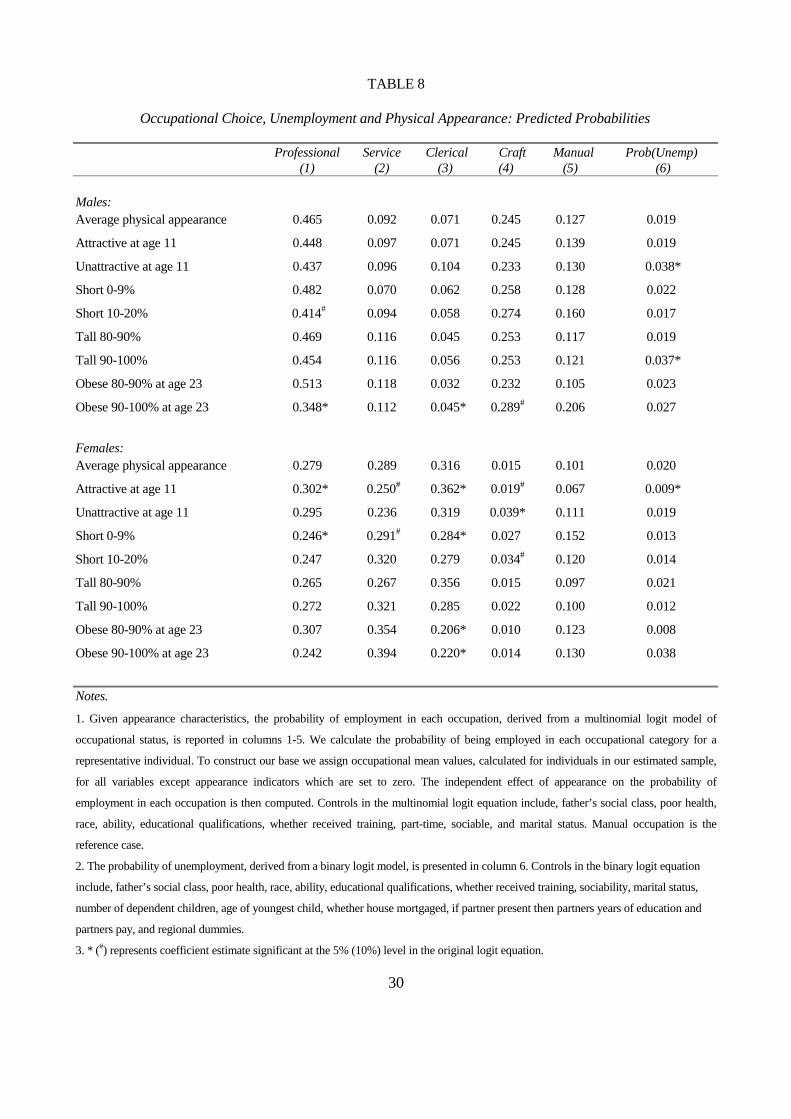
As coefficient estimates of the binary logit model are difficult to interpret we calculate the

probability of being unemployed for a representative individual assigned sample mean values for all

variables except for indicators for appearance which are set to zero. The effect of appearance on the

probability of unemployment, calculated from the binary logit estimates, are presented in column 6 of

Table 8. We find some evidence in support of pure employer discrimination in that the probability of

unemployment rises by 1.9 percentage points for unattractive men but falls from 2% to 0.9% for

attractive women. Very tall men in the 90+ percentile range are also more likely to be unemployed. All

other quantitative effects are comparatively small and statistically insignificant.

Conversely, if occupations reward appearance differently, as a result of productivity effects,

then differences in expected earnings will affect occupational choice (Robertson and Symons, 1990)

and occupational mobility (Harper, 1995). We investigate this possibility by estimating a multinomial

logit model of occupational status which includes physical appearance. To summarise our results we

20 Estimating a multinomial model we find no significant effects of appearance on the probability of being self-employed

relative to being employed.

15

calculate the probability of being employed in a broad occupational category for a representative

individual. To construct our base we assign occupational mean values, calculated for individuals in our

estimated sample, for all variables except appearance indicators which are set to zero. The independent

effect of appearance on the probability of employment in each occupation is then computed. Results

are reported in Table 8, columns 1-5.

Our results indicate that physical appearance causes significant differences in the probability of

being employed in an occupation. For example, the probability of working in professional or clerical

occupations is significantly higher for attractive women. Also, men and women who are relatively

short or obese are less likely to be employed in, respectively, professional and clerical occupations21.

In addition, we expect individuals to sort into occupations that reward a particular attribute and

away from occupations where penalties exist. The results in Table 8 are broadly consistent with our

estimates of pay differentials associated with physical appearance presented in Table 7. All probability

estimates change in the expected direction except for attractiveness for men having no effect on the

probability of employment in craft occupations and women who are unattractive being slightly more

likely to be employed in a clerical occupation. However, in the latter case, attractiveness raises the

probability, ceteris paribus, of being in a clerical occupation by 4.6 percentage points.

The results of this section show that those assessed as unattractive as children fare less well in

the labour market in adulthood while children assessed as attractive obtain significant economic

advantage. How are these results to be interpreted? One explanation is that we are measuring, with

21Hamermesh and Biddle (1994) find some evidence for occupational sorting arising from attractiveness but conclude that

the effects are generally small.

16

error, beauty at age 33. Hatfield and Sprecher (1986) report evidence of stability in the assessment of

an individual’s appearance at different stages of their adult lives. We are not aware, however, of any

evidence that examines the stability of appearance ratings from childhood into adulthood. Indirect

evidence, that assessments of attractiveness in childhood are a proxy for attractiveness at age 33, is

reported later in Section V where we find significant effects for our attractiveness variables in the

marriage market.

Another possible explanation for our results is that the assessment of attractiveness, and other

appearance variables, are correlated with unobserved productivity. We report earlier, for example, how

assessments of appearance are not independent of ability and sociability. However the effects of

appearance on pay continue to be observed in our preferred final equations after controlling for these

variables plus an extensive set of additional controls. As an additional test we examine whether

physical appearance, psychological development and earnings may be related22.We test for this by

including an indicator for depression23 in the earnings equations reported in Table 6, columns 3 and 6.

For both males and females the effects on the estimated coefficients are very small and the indicator

for depression is always insignificant. However, as is always the case in this type of study, we cannot

reject the possibility that all our measures of appearance are correlated with unobserved productive

attributes which affect earnings.

V. PHYSICAL APPEARANCE, MARRIAGE, AND FAMILY LABOUR INCOME

22For example, obesity may be associated with some psychological disorders (Kannel, 1983) which may be correlated with

unobserved productivity.23Calculated for the respondent at age 23 from a ‘malaise’ score, derived from a 26-item self-completed questionnaire,

developed by Rutter et al. (1970). A score of seven or more is suggested to be an indication of depression.

17

Physical appearance may, in addition to its effects on earnings and employment, also affect an

individual’s family income by altering opportunities for marriage and the earnings of a partner.

Derivatives, evaluated at sample means, calculated from a binary logit equation relating marriage to

physical appearance24, are reported in Table 9, columns 1 and 3. Controls include social class,

education, health, race, and region of residence. In heterosexual couples, men are much more likely to

be taller than their female partner than would arise from random matching (Gillis and Avis, 1980). Our

results show that the probability of being married is 7 percentage points lower for short men and 5

percentage points lower for tall women, indicating that short males and tall females may experience

greater difficulty in finding a suitable match. Also, the partners of tall men appear to earn around 15%

more than those in the reference group (Table 9, column 4). Unattractive men are less likely to be

married while attractive women are more likely to be married. However, attractiveness has no

significant effect on partner’s pay.

For women, obesity imposes significant economic costs in terms of the likelihood of marriage

and partner’s income. The likelihood of marriage for obese women in the 90+ percentile category is 7

percentage points lower than the reference group and partners earn 15% less. Similar to findings for

the USA (Averett and Korenman, 1996), we find that the greater part of the economic disadvantage

associated with obesity among women results from disadvantage in the marriage market.

From our estimated equations we present in Table 10 predicted differences in household

income, accruing from the labour market and marriage, for selected categories relative to household

income for males or females, and their potential partners, with average physical appearance and who

are assumed to receive sample full-time average earnings. The largest absolute and relative penalties

24Marriage in NCDS is defined as currently married or living as married.

18

for physical appearance accrue to unattractive men and obese women. Unattractive men, however,

experience most of their income disadvantage from the labour market while, for obese women, a

substantial part of the household income penalty arises from a lower probability of marriage and,

where married, lower expected earnings of a partner.

VI. SUMMARY AND CONCLUSIONS

In accord with previous studies, our results indicate that, contrary to popular belief, physical

appearance is as important for men as it is for women. In particular, we find that, irrespective of

gender, those who are assessed as unattractive or of short stature experience significant earnings

disadvantage. Tall men receive a pay premium while obese women experience a pay penalty. The

impact of physical appearance is also evident in the marriage market. Among women, those who are

tall or obese are less likely to be married; while among men, lower marriage rates are found for those

who are short or unattractive. If assessments of the attractiveness of individuals remain stable over

time then our results provide estimates of the economic returns to beauty in the labour market.

Our results indicate that the bulk of the pay differential for appearance arises from employer

discrimination. The probability of unemployment increasing for unattractive men but decreasing for

attractive women provides additional support for employer discrimination. However, we also find

evidence which is consistent with productivity differences arising from either physical productivity or

from customer discrimination. Earnings differentials for appearance, especially attractiveness, vary

among occupations. As additional support we find evidence for sorting across occupations arising

19

from physical appearance. The differential effects of appearance for women in clerical/secretarial

occupations are substantial.

Distinguishing the proportion of the earnings differential which may be attributed to

discrimination, as opposed to greater productivity, is problematic. However, our conclusion that the

bulk of the estimated pay differential arising from physical appearance is due to employer

discrimination appears to be quite robust. Further investigation of this result for other economies

would be beneficial.

London Guildhall University

REFERENCES

Averett, S. and Korenman, S. (1996). ‘The Economic Reality of The Beauty Myth’, Journal of

Human Resources, Vol. 31, pp. 304-30.

Becker, G. (1957). The Economics of Discrimination, Chicago University Press, Chicago.

Boldsen, J.L. and Mascie-Taylor, C.G.N. (1985). ‘Analysis of Height Variation in a Contemporary

British Sample’, Human Biology, Vol. 57, pp. 473-80.

Connolly, S., Micklewright, J., and Nickell, S. (1992).‘The Occupational Success of Young Men

Who Left School at Sixteen’, Oxford Economic Papers, Vol. 44, pp. 460-79.

Eisenberg, N., Roth, K., Bryniarski, K.A., and Murray, E. (1984). ‘ Sex Differences in the

Relationship of Height to Children’s Actual and Attributed Social and Cognitive

Competencies’, Sex Roles, Vol. 11, pp. 719-34.

20

Felson, R.B. and Bohrnstedt, G.W. (1979). ‘"Are the Good Beautiful or The Beautiful Good ?" The

Relationship Between Children's Perceptions of Ability and Perceptions of Physical

Attractiveness’, Social Psychology Quarterly, Vol. 42, pp. 386-92.

Gillis, J.S. and Avis, W.E. (1980). ‘The Male-Taller Norm in Mate Selection’, Personality and Social

Psychological Bulletin, Vol. 6, pp. 396-401.

Hamermesh, D.S. and Biddle, J.E. (1994). ‘Beauty and the Labor Market’, American Economic

Review, Vol. 84, pp. 1174-94.

Hamermesh, D.S. and Biddle, J.E. (1998). ‘Beauty, Productivity, and Discrimination: Lawyers’ Looks

and Lucre’, Journal of Labour Economics, Vol. 16, pp. 172-201.

Harper, B.A. (1995). ‘Male Occupational Mobility in Britain’, Oxford Bulletin of Economics and

Statistics, Vol. 57, pp. 349-69.

Harper, B.A. and Haq, M. (1997). ‘Occupational Attainment of Men in Britain’, Oxford Economic

Papers, Vol. 49, pp. 638-50.

Hatfield, E. and Sprecher, S. (1986). Mirror, Mirror....: The Importance of Looks in Everyday Life,

State University of New York Press, Albany.

Jackson, L.A., Hunter, J.E., Hodge, C.N. (1995). ‘Physical Attractiveness and Intellectual

Competence: A Meta-Analytic Review’, Social Psychology Quarterly, Vol. 58, pp. 108-22.

Lee, L. (1983). ‘Generalized Models of Selectivity’, Econometrica, Vol. 51, pp. 507-12.

Lynn, R. (1989). ‘A Nutrition Theory of the Secular Increases in Intelligence; Positive Correlations

Between Height, Head Size and IQ’, British Journal of Educational Psychology, Vol. 59,

pp. 372-7.

Kannel, W. (1983). ‘Health and Obesity: An Overview’, in H.L. Conn, E.A. DeFelice, and P.T. Kuo

(eds), Health and Obesity, Raven, New York.

21

Loh, E.S. (1993). ‘The Economic Effects of Physical Appearance’, Social Science Quarterly, Vol. 74,

pp. 420-38.

Martel, L.F. and Biller, H.B. (1987). Stature and Stigma, D.C. Heath and Company, Lexington.

Robertson, D. and Symons, J. ‘The Occupational Choice of British Children’, Economic Journal,

Vol. 100, pp. 828-41.

Rutter, M., Tizard,J., and Whitmore, K. (1970). Education, Health and Behaviour, Longman, London.

Sargent, J.D. and Blanchflower, D.G. (1994). ‘Obesity and Statute in Adolescence and Earnings in

Young Adulthood: Analysis of a British Birth Cohort’, Archives of Pediatrics and Adolescent

Medicine, Vol. 148, pp. 681-7.

Sobal, J. and Stunkard, A.J. (1989). ‘Socioeconomic Status and Obesity: A Review of the Literature’,

Psychological Bulletin, Vol. 105, pp. 260-75.

Sorensen, T.I. and Sonne-Holm, S. (1985). ‘Intelligence Test Performance in Obesity in Relation to

Educational Attainment and Parental Social Class’, Journal of Biosocial Science, Vol. 17,

pp. 379-87.

Waldfogel, J. (1995). ‘The Price of Motherhood: Family Status and Women’s Pay in a Young British

Cohort’, Oxford Economic Papers, Vol. 47, pp. 584-610.

22

TABLE 1

Selected Variable Means by Physical Appearance: Male Employees

Variable Allemployees

Attractive(age 11)

Unattractive(age 11)

Short(0-9%)

Tall(90-100%)

Obese(90-100%)

Hourly wage (£) 7.792 8.239 6.893 6.770 8.341 6.794Attractive (age 11) 0.454 1.000 0.000 0.360 0.447 0.335Unattractive (age 11) 0.075 0.000 1.000 0.088 0.060 0.105Body Mass Index 25.551 25.401 26.237 25.894 25.085 30.982Body Mass Index age 23 23.064 22.950 23.409 23.015 22.960 28.853Height (meters) 1.770 1.773 1.766 1.654 1.890 1.766Father’s social class I (birth) 0.051 0.054 0.035 0.035 0.082 0.012Father’s social class II (birth) 0.137 0.148 0.099 0.093 0.156 0.077Father’s social class III (birth) 0.621 0.633 0.602 0.629 0.633 0.660Father’s social class IV (birth) 0.115 0.106 0.134 0.139 0.071 0.156Ability (age 11) 8.836 9.359 7.842 7.691 9.655 7.635Apprenticeship 0.049 0.043 0.057 0.042 0.034 0.051O’ Levels 0.259 0.263 0.244 0.289 0.280 0.302A’ Levels 0.214 0.228 0.176 0.214 0.197 0.222HND / Teaching 0.137 0.153 0.107 0.097 0.143 0.088Graduate 0.155 0.170 0.118 0.108 0.209 0.046Firm tenure in years 7.650 7.805 6.771 7.428 7.583 8.079Work experience: years 23-33 10.413 10.481 10.208 10.323 10.36 10.477Trade union member 0.437 0.448 0.410 0.449 0.410 0.454Work related training 0.505 0.526 0.418 0.452 0.548 0.436Part-time employee 0.010 0.009 0.013 0.017 0.007 0.014Poor health 0.009 0.008 0.006 0.014 0.012 0.011Respondent white 0.978 0.985 0.981 0.957 0.995 0.980Sociable (age 16) 0.212 0.245 0.147 0.189 0.201 0.201Depression (age 23) 1.030 1.023 1.042 1.033 1.034 1.057House mortgaged 0.743 0.787 0.640 0.647 0.757 0.667Married 0.820 0.836 0.783 0.748 0.829 0.827Partner left school age 17-182 0.245 0.259 0.171 0.213 0.249 0.183Partner left school age 19 plus 0.170 0.188 0.117 0.094 0.255 0.078Partner’s net weekly pay3 121.429 118.028 111.619 105.289 138.510 107.022Number of children: 1 0.199 0.199 0.196 0.172 0.198 0.205 2 0.355 0.379 0.329 0.338 0.339 0.327 3+ 0.131 0.121 0.150 0.172 0.102 0.153Age of youngest child 3.157 3.074 3.314 3.450 2.859 3.752Professional occupation 0.421 0.459 0.320 0.347 0.480 0.255Service occupation 0.113 0.122 0.070 0.093 0.153 0.128Clerical occupation 0.062 0.062 0.077 0.069 0.055 0.048Craft occupation 0.217 0.195 0.280 0.279 0.168 0.264Manual occupation 0.186 0.162 0.253 0.213 0.143 0.306Sample size 4160 1889 313 422 416 352

Notes: 1. Data refer to respondents at age 33 unless otherwise stated. 2. Partner’s education, if respondent is married. 3. Annual earnings of partner, if respondent is married and partner in employment.

23

TABLE 2

Selected Variable Means by Physical Appearance: Female Employees

Variable Allemployees

Attractive(age 11)

Unattractive(age 11)

Short(0-9%)

Tall(90-100%)

Obese(90-100%)

Hourly wage (£) 5.591 5.749 5.085 4.888 6.153 4.831Attractive (age 11) 0.564 1.000 0.000 0.442 0.617 0.439Unattractive (age 11) 0.078 0.000 1.000 0.088 0.054 0.165Body Mass Index 24.578 24.121 26.857 25.309 24.131 32.336Body Mass Index (age 23) 22.184 21.913 23.785 22.738 21.791 29.181Height (meters) 1.630 1.634 1.618 1.515 1.747 1.617Father’s social class I (birth) 0.044 0.048 0.023 0.019 0.069 0.018Father’s social class II (birth) 0.135 0.140 0.121 0.096 0.177 0.082Father’s social class III (birth) 0.617 0.626 0.607 0.609 0.600 0.630Father’s social class IV (birth) 0.127 0.121 0.160 0.159 0.098 0.192Ability at age 11 8.835 9.270 7.674 8.000 10.058 7.802Apprenticeship 0.039 0.043 0.037 0.047 0.031 0.040O’ Levels 0.368 0.381 0.401 0.319 0.356 0.360A’ Levels 0.102 0.113 0.074 0.097 0.140 0.096HND / Teaching 0.138 0.150 0.087 0.093 0.158 0.125Graduate 0.122 0.131 0.074 0.105 0.182 0.043Firm tenure in years 5.486 5.452 5.606 5.354 5.539 5.671Work experience: years 23-33 8.788 8.869 8.653 8.395 9.080 8.658Trade union member 0.358 0.363 0.339 0.332 0.407 0.342Work related training 0.348 0.371 0.303 0.316 0.435 0.247Part-time employee 0.468 0.465 0.466 0.517 0.380 0.459Poor health 0.012 0.009 0.022 0.007 0.003 0.037Respondent white 0.981 0.985 0.989 0.962 0.982 0.990Sociable (age 16) 0.261 0.285 0.142 0.255 0.307 0.214Depression (age 23) 1.089 1.080 1.124 1.121 1.085 1.146House mortgaged 0.737 0.768 0.656 0.670 0.741 0.621Married 0.794 0.802 0.792 0.765 0.728 0.742Partner left school age 17-18 0.160 0.166 0.135 0.143 0.156 0.116Partner left school age 19 plus 0.174 0.186 0.145 0.143 0.269 0.084Partner’s net weekly pay 270.020 278.528 226.501 256.287 264.061 202.247Number of children: 1 0.200 0.202 0.190 0.161 0.207 0.159 2 0.387 0.386 0.364 0.431 0.344 0.437 3+ 0.141 0.137 0.171 0.146 0.126 0.173Age of youngest child 4.651 4.546 5.430 5.412 4.011 5.827Professional occupation 0.346 0.366 0.282 0.298 0.430 0.280Service occupation 0.239 0.225 0.263 0.256 0.201 0.294Clerical occupation 0.275 0.298 0.237 0.253 0.282 0.226Craft occupation 0.019 0.018 0.034 0.032 0.013 0.034Manual occupation 0.121 0.093 0.184 0.161 0.075 0.166Sample size 3541 1998 275 294 334 303

Notes: 1. See notes to Table 1.

24

TABLE 3

Gender Distributions of Beauty: Attractiveness Categories at Age 11

by Attractiveness Categories at Age 7

Attractive

Age 11

Average Unattractive All N

Age 7Males: Attractive 53.8 40.6 5.6 51.4 2879

Average 36.7 54.1 9.7 41.8 2345

Unattractive 23.6 54.1 21.8 6.8 381

All 44.6 47.2 8.2 100.0

N 2501 2644 460 5605

Females: Attractive 64.8 29.1 6.1 57.3 3322

Average 46.4 43.2 10.3 35.9 2079

Unattractive 33.2 44.8 21.9 6.8 397

All 56.0 35.3 8.7 100.0

N 3250 2045 503 5798

25

TABLE 4

Mean Hourly Earnings by Occupation and Physical Appearance

Total Attractive Unattractive Short

(0-9%)

Tall

(80-89%)

Tall

(90-100%)

Obese

(90-100%)

Males:

Professional 9.934 9.989 8.779 8.631 10.136 9.692 8.722

Service 7.353 7.709 6.372 5.976 7.990 7.762 7.097

Clerical 7.135 6.969 6.284 6.213 7.636 7.308 6.586

Craft 6.419 6.442 6.150 6.107 6.777 7.017 6.123

Manual 5.636 6.055 5.503 5.335 5.368 6.307 5.469

Females:

Professional 7.772 7.783 7.588 7.139 8.022 7.601 7.103

Service 3.797 3.768 3.955 3.530 3.408 4.345 3.722

Clerical 5.302 5.388 4.539 4.946 5.363 5.792 4.578

Craft 4.120 4.194 3.717 3.496 4.775 2.800 3.755

Manual 3.516 3.522 3.455 3.208 3.668 3.927 3.568

26

TABLE 5

Physical Appearance And Economic Activity

Total Attractive Unattractive Short

(0-9%)

Tall

(80-89%)

Tall

(90-100%)

Obese

(90-100%)

Males:

Economically Active 0.964 0.974 0.945 0.932 0.957 0.967 0.951

Self-employed 0.160 0.170 0.147 0.150 0.140 0.141 0.126

Employed 0.745 0.758 0.686 0.698 0.776 0.762 0.749

Unemployed 0.060 0.046 0.112 0.084 0.041 0.064 0.077

Females:

Economically Active 0.700 0.706 0.649 0.664 0.724 0.719 0.699

Self-employed 0.067 0.075 0.066 0.052 0.083 0.074 0.057

Employed 0.613 0.617 0.551 0.592 0.625 0.617 0.616

Unemployed 0.020 0.014 0.032 0.020 0.016 0.028 0.026

27

TABLE 6

Physical Appearance and Earnings

Males

(1) (2) (3)

Females

(4) (5) (6)

Attractive (age 7 & 11) 0.112 0.006 0.005 0.064 0.006 -0.023

(5.14)* (0.25) (0.23) (2.63)* (0.19) (-0.88)

Attractive (age 11 only) 0.058 -0.017 -0.006 0.011 -0.027 -0.031

(2.35)* (-0.60) (-0.21) (0.42) (-0.86) (-1.08)

Attractive (age 7 only) 0.053 -0.017 -0.010 0.014 -0.013 -0.033

(2.47)* (-0.68) (-0.42) (0.52) (-0.39) (-1.08)

Unattractive (age 7&11) -0.124 -0.193 -0.149 -0.171 -0.114 -0.109

(-1.91)# (-2.56)* (-2.08)* (-2.90)* (-1.81)# (-1.90)#

Unattractive (age 11 only) -0.066 -0.063 -0.040 -0.026 0.002 0.016

(-2.07)* (-1.83)# (-1.30) (-0.71) (0.05) (0.44)

Unattractive (age 7 only) -0.128 -0.089 -0.027 -0.074 -0.023 -0.049

(-3.70)* (-2.20)* (-0.73) (-2.18)* (-0.60) (-1.27)

Short 0-9% -0.094 -0.058 -0.043 -0.073 -0.096 -0.051

(-3.80)* (-2.04)* (-1.71)# (-2.42)* (-2.84)* (-1.72)#

Short 10-19% -0.057 -0.049 -0.038 -0.000 0.009 0.051

(-2.09)* (-1.61) (-1.41) (-0.01) (0.30) (1.79)#

Tall 80-89% 0.084 0.075 0.059 -0.001 -0.006 0.012

(3.11)* (2.47)* (2.08)* (-0.02) (-0.19) (0.44)

Tall 90-100% 0.062 0.052 0.017 0.066 0.024 -0.035

(2.43)* (1.71)# (0.60) (2.33)* (0.73) (-1.20)

Obese 80-89% (age 23) -0.009 0.013 -0.002 -0.063 -0.048 -0.050

(-0.32) (0.45) (-0.07) (-2.07)* (-1.41) (-1.66)#

Obese 90-100% (age 23) -0.084 -0.049 -0.009 -0.097 -0.076 -0.053

(-3.53)* (-1.70)# (-0.32) (-3.56)* (-2.59)* (-1.91)#

Sociable (age 16) 0.095 0.064 0.052 0.031

(4.72)* (3.52)* (2.46)* (1.62)

Ability (age 11) 0.039 0.010 0.040 0.010

(16.09)* (3.74)* (14.17)* (3.11)*

28

TABLE 6---continued

Physical Appearance and Earnings

Males

(1) (2) (3)

Females

(4) (5) (6)

Social class dummies (4) Yes Yes Yes Yes Yes Yes

Poor Health Yes Yes Yes Yes Yes Yes

Race Yes Yes Yes Yes Yes Yes

Educational dummies (5) No No Yes No No Yes

Other individual characteristics No No Yes No No Yes

Firm size dummies (3) No No Yes No No Yes

Occupational dummies (4) No No Yes No No Yes

Industry dummies (15) No No Yes No No Yes

Regional dummies (11) No No Yes No No Yes

R 2 0.093 0.198 0.426 0.247 0.330 0.581

N 2820 2002 1693 2421 1695 1271

Notes:

1. The dependent variable is log(hourly earnings) at age 33.

2. Controls included under ‘other individual characteristics’ are: part-time employee, firm tenure, work experience between

age 23 and age 33, whether training received, trade union membership, and marital status.

3. T-statistics are in parentheses. * (#) represents significant at the 5% (10%) level.

4. The reference group for the reported coefficients is: attractiveness assessed as average at both age 7 and age 11, 20-79

percentile range for height and 0-79 percentile range for weight at age 23. In addition, in columns 2, 3, 5 and 6, the

reference group includes not assessed as being relatively sociable at age 16.

29

TABLE 7

Physical Appearance, Occupation, and Earnings

Males

(1) (2)

Females

(3) (4)

Attractive (age 11) 0.008 0.053 -0.006 -0.007

(0.48) (2.19)* (-0.29) (-0.36)

Unattractive (age 11) -0.057 -0.111 0.006 0.052

(-1.95)# (3.20)* (0.17) (1.34)

Short 0-9% -0.044 -0.047 -0.051 -0.055

(-1.73)# (-1.85)# (-1.74)# (-1.86)#

Tall 80-89% 0.060 0.081 0.014 0.012

(2.10)* (2.52)* (0.51) (0.435)

Obese 90-100% (age 23) -0.009 -0.007 -0.054 -0.042

(-0.33) (-0.27) (-1.94)# (-1.49)

Prof/attractive -0.061

(-1.75)#

Craft/attractive -0.089

(-2.18)#

Manual/unattractive 0.213

(3.55)*

Clerical/unattractive -0.146

(-2.30)*

Manual/tall 80-90% -0.122

(-2.13)*

Craft/obese 90-100% -0.306

(-2.93)*

R 2 0.426 0.426 0.581 0.583

N 1693 1693 1271 1271

Notes:

1. See notes 1-3 for Table 6. Non-physical appearance controls are identical to those in Table 6, columns 3 and 6.

2. The reference group for the reported coefficients is: attractiveness assessed as average at age 11, 20-79 percentile range

for height and 0-79 percentile range for weight at age 23.

3. Occupations are: professional, service, clerical, craft and manual.

30

TABLE 8

Occupational Choice, Unemployment and Physical Appearance: Predicted Probabilities

Professional(1)

Service(2)

Clerical(3)

Craft(4)

Manual(5)

Prob(Unemp) (6)

Males:Average physical appearance 0.465 0.092 0.071 0.245 0.127 0.019

Attractive at age 11 0.448 0.097 0.071 0.245 0.139 0.019

Unattractive at age 11 0.437 0.096 0.104 0.233 0.130 0.038*

Short 0-9% 0.482 0.070 0.062 0.258 0.128 0.022

Short 10-20% 0.414# 0.094 0.058 0.274 0.160 0.017

Tall 80-90% 0.469 0.116 0.045 0.253 0.117 0.019

Tall 90-100% 0.454 0.116 0.056 0.253 0.121 0.037*

Obese 80-90% at age 23 0.513 0.118 0.032 0.232 0.105 0.023

Obese 90-100% at age 23 0.348* 0.112 0.045* 0.289# 0.206 0.027

Females:Average physical appearance 0.279 0.289 0.316 0.015 0.101 0.020

Attractive at age 11 0.302* 0.250# 0.362* 0.019# 0.067 0.009*

Unattractive at age 11 0.295 0.236 0.319 0.039* 0.111 0.019

Short 0-9% 0.246* 0.291# 0.284* 0.027 0.152 0.013

Short 10-20% 0.247 0.320 0.279 0.034# 0.120 0.014

Tall 80-90% 0.265 0.267 0.356 0.015 0.097 0.021

Tall 90-100% 0.272 0.321 0.285 0.022 0.100 0.012

Obese 80-90% at age 23 0.307 0.354 0.206* 0.010 0.123 0.008

Obese 90-100% at age 23 0.242 0.394 0.220* 0.014 0.130 0.038

Notes.

1. Given appearance characteristics, the probability of employment in each occupation, derived from a multinomial logit model of

occupational status, is reported in columns 1-5. We calculate the probability of being employed in each occupational category for a

representative individual. To construct our base we assign occupational mean values, calculated for individuals in our estimated sample,

for all variables except appearance indicators which are set to zero. The independent effect of appearance on the probability of

employment in each occupation is then computed. Controls in the multinomial logit equation include, father’s social class, poor health,

race, ability, educational qualifications, whether received training, part-time, sociable, and marital status. Manual occupation is the

reference case.

2. The probability of unemployment, derived from a binary logit model, is presented in column 6. Controls in the binary logit equation

include, father’s social class, poor health, race, ability, educational qualifications, whether received training, sociability, marital status,

number of dependent children, age of youngest child, whether house mortgaged, if partner present then partners years of education and

partners pay, and regional dummies.

3. * (#) represents coefficient estimate significant at the 5% (10%) level in the original logit equation.

31

TABLE 9

Physical Appearance, Marriage and Partner’s Income

Females

Prob (married) Ln (partner’s pay)

(1) (2)

Males

Prob(married) Ln (partner’s pay)

(3) (4)

Attractive (age 7 & 11) 0.037# 0.031 (0.80) 0.026 -0.061 (0.98)

Attractive (age 11 only) 0.002 0.018 (0.46) 0.011 -0.035 (0.53)

Attractive (age 7 only) 0.036 0.069 (1.59) 0.013 -0.019 (0.30)

Unattractive (age 7 & 11) -0.029 0.049 (0.42) -0.085# 0.037 (0.22)

Unattractive (age 11 only) 0.007 -0.020 (0.46) -0.005 -0.097 (1.20)

Unattractive (age 7 only) 0.021 -0.063 (1.20) -0.005 -0.094 (1.13)

Short 0-9% -0.031 -0.031 (0.70) -0.067* 0.046 (0.70)

Short 10-19% -0.005 -0.072 (2.04)* -0.026 0.029 (0.42)

Tall 80-89% -0.037 -0.067 (1.54) -0.014 0.057 (0.79)

Tall 90-100% -0.052* 0.005 (0.12) 0.005 0.147 (2.25)*

Obese 80-89% -0.001 -0.020 (0.55) 0.001 -0.140 (2.01)*

Obese 90-100% -0.066* -0.145 (4.61)* 0.010 -0.018 (0.26)

R2 or Pseudo R2 0.024 0.112 0.022 0.137

N 3117 1822 2918 1317

Notes:

1. The logit equations for marriage (columns 1 and 3) and the regressions for partner’s earnings (columns 2 and 4) include

the following controls; father’s social class, race, ability, sociable, poor health, highest educational qualification obtained,

and region of residence.

2. Numbers shown in all logit equations are derivatives evaluated at the sample mean and may be interpreted as percentage

point differences in the relevant probability.

3. T-statistics are in parentheses . * (#) represents significant at the 5% (10%) level.

32

TABLE 10

Physical Appearance and Annual Income Differences

(£ at 1991 prices)

Unattractive

men

Unattractive

women

Tall Men

(80-89%)

Short Men

(0-9 %)

Obese women

(90%+)

Labour market -2229 -1170 883 -643 -569

Marriage market -621 +127 343 -347 -2,567

Total income differential -2850 -1043 1,226 -990 -3,136

Total expected household

income

23,763 22,614 23,763 23,763 22,614

% differential -12.0% -4.6% 5.1% -4.2% -13 .9%

Notes:

1. For the base case we assume that individuals work for 40 hours per week and 48 weeks per year. Males and females

receive sample average full-time earnings for their gender.