WORKING PAPERS

Working Paper No 2011-62 December 2011

Beauty and the beast in the labor market:

A distribution regression approach

Karina DOORLEYEva SIERMINSKA

CEPS/INSTEAD Working Papers are intended to make research findings available and stimulate comments and discussion. They have been approved for circulation but are to be considered preliminary. They have not been edited and have not

been subject to any peer review.

The views expressed in this paper are those of the author(s) and do not necessarily reflect views of CEPS/INSTEAD. Errors and omissions are the sole responsibility of the author(s).

Beauty and the beast in the labor market:Evidence from a distribution regression

approach∗

Karina Doorley†CEPS/INSTEAD, Luxembourg and University College Dublin

Eva Sierminska‡CEPS/INSTEAD, Luxembourg and DIW Berlin

December 2011

Abstract

We apply an innovative technique to allow for differential effects of physicalappearance across the wage distribution, as traditional methods confound opposingeffects. Counterfactual wage distributions constructed using distribution regression,show that unattractive women are more likely to earn less than the median wage,particularly in professions where physical appearance is important. We also finda premium for well-paid attractive men in these professions. A comparison withresults from traditional models shows that the characteristics of people in differentphysical appearance classes contributes to the effects identified using the latter andonly a small portion could be discrimination.

Keywords: Wages; Distribution; Physical Appearance; DiscriminationJEL classification codes: D31; J24; J30; J70

∗The authors would like to thank Ronald Oaxaca, Philippe Van Kerm and the participants of the C/Iseminar series for helpful suggestions and comments. This research is part of the MeDIM project Advancesin the Measurement of Discrimination, Inequality and Mobility) supported by the Luxembourg ‘Fonds Na-tional de la Recherche’ (contract FNR/06/15/08) and by core funding for CEPS/INSTEAD by the Ministryof Higher Education and Research of Luxembourg.†Karina Doorley, CEPS/INSTEAD, 3, avenue de la Fonte, L-4364 Esch-sur-Alzette, Luxembourg.

Phone: +352 585855. Fax: +352 585560. E-mail: karina.doorley@ceps.lu.‡Eva Sierminska, CEPS/INSTEAD, 3, avenue de la Fonte, L-4364 Esch-sur-Alzette, Luxembourg.

Phone: +352 585855409. Fax: +352 585560. E-mail: eva.sierminska@ceps.lu.

1

’All that glitters is not gold’ -W. Shakespeare

1 Introduction

Like in so many areas of life, Shakespeare had excellent insight into the sometimes mis-leading effects of physical appearance. In this paper, we examine whether the glitter ofan appealing physical appearance leads to higher pay. It has been shown that beauty ispositively related to earnings in the labor market. Hamermesh and Biddle (1994), in theirseminal paper, show the existence of an average wage penalty of 5-10% for being plainand an average wage premium of 5-10% for being beautiful in the US and Canada. Mostother studies that find a positive effect of looks on earnings also identify average effects(Biddle and Hamermesh (1998), Harper (2000), Hamermesh et al. (2002), Mobius andRosenblat (2006) and Sen et al. (2010)). While measuring average effects is quite infor-mative and convenient, it also has substantial drawbacks, as opposing effects that existacross the distribution may be confounded in the summary effect. This has already beendiscovered for other variables that affect wages, such as gender, for example (Bonjour andGerfin (2001)). As far as we know, the varying effect of beauty on wages throughout thedistribution has not been examined. The effect may vary across the distribution becausedifferent points of the distribution correspond to different job types, which pay a differentpremium for looks. Better looking people, ceteris paribus, may have more opportunitiesto advance and have higher wages, while less good looking people may need to com-pensate with their qualifications and other traits, and the extent of these differences mayvary depending on where the individual is located in the distribution. In this paper, ourgoal is to examine the effect of beauty on earnings across the wage distribution using aninnovative technique and new data.

Our contribution to the literature is three-fold. First, we demonstrate that the effect ofbeauty varies across the wage distribution. Next, we demonstrate how distribution regres-sion, a method seldom used in this literature and initially used to model excess returns onfinancial markets, could prove a useful tool in decomposing wage differentials by physicalappearance across the wage distribution. Finally, given that data on physical appearanceis fairly scarce, having access to a unique dataset, we provide new results on the effect ofbeauty on wages in a new country.

Our strategy is as follows. We start by estimating a Heckman selection model for wagesat the mean. Next, suspecting that there is some variation in the effect of physical appear-ance in different areas of the wage distribution, we estimate a series of quantile regressions

(QR) to serve as a benchmark. Finally, discovering that there is indeed variation acrossthe distribution, we progress to distribution regression (DR) to model counterfactual dis-tributions of wages for groups of people classed by physical appearance. Modeling wagedistributions using DR is related to QR in that DR models the conditional probability ofbeing located in particular quantile group while QR models the conditional wage of a par-ticular quantile group. We model entire counterfactual distributions of wages, in order topinpoint wage gaps between different groups of people at every point of the distribution.An Oaxaca-Blinder style decomposition of these counterfactual distributions allows us toidentify the existence or absence of beauty premia and plain penalties. We show that thereare indeed differences in the effect of beauty across the earnings distribution. The effectvaries for men and women and by occupations. We apply these three methodologies to aunique dataset from Luxembourg.

In Section 2 we provide some background information on prior modeling of the effect ofphysical appearance on various outcome variables and the previous literature. In Section3 we outline our methodology. Section 4 describes the data and variable construction.Section 5 discusses the results and Section 7 concludes.

2 Background

Biddle and Hamermesh (1998), Harper (2000), Hamermesh et al. (2002), Mobius andRosenblat (2006) and Sen et al. (2010), using different methods, all find evidence of apositive relationship between physical appearance and earnings. This relationship hasbeen shown to be different for men and women. A theoretical framework on this issue isoffered by Jackson (1992). In her model, both the sociobiological (reproductive potential)and sociocultural (cultural values) perspectives predict that physical attractiveness hasgreater implications for females than males. A number of other studies have validated this.Frieze et al. (1991), for example consider the relationship between facial attractivenessand income. They discover that attractive males are able to secure higher starting salariesand that the earnings differentials are persistent over time. The most attractive femalegraduates do not earn higher starting salaries but they do earn more income later in theircareers.

There are a number of possible explanations for the relationship between physical appear-ance and earnings. These have been categorized into direct and indirect effects. Directeffects, first elaborated by Hamermesh and Biddle (1994), include pure employer dis-crimination, customer discrimination and occupational crowding. The indirect effects are

2

harder to pin down but a number of theories have been put forward. Mocan and Tekin(2010) find evidence that being an unattractive student in high school may hinder humancapital development due to preferential treatment. This will have a knock-on effect onearnings later in life. There are also effects through the marriage market. Barro (1998)finds that less attractive women are much less likely to marry than attractive women andtend to have husbands with sharply lower earnings. While this does not directly affect thewoman’s earnings, it does affect total household earnings.

3 Methodology

As a first step of our empirical strategy, we will test the hypotheses put forth by Hamer-mesh and Biddle (1994), at the mean, controlling for selection into employment, and usingdifferent quantile groups. We then apply the DR approach pioneered by Foresi and Per-acchi (1995) to examine the effect of beauty across the whole earnings distribution. Weconstruct flexible counterfactual wage distributions, using the group of men and womenwith self-assessed average physical appearance as the baseline, to see whether differencesacross beauty groups are driven by differences in characteristics or differences in the wagefunction (coefficients).

3.1 Hamermesh and Biddle selection model

Hamermesh and Biddle (1994) put forward three possible reasons for earnings differen-tials based on physical appearance: customer discrimination, employer discrimination,and occupational sorting. The first of these assumes that looks may enhance productivityat work. In this case, physical appearance may enhance the worker’s ability to engage inproductive interactions with coworkers or customers in certain occupations because theyprefer interacting with better looking individuals. In this framework there will be a pre-mium for good looks and workers will sort into the occupation paying the highest wage.Attractive and unattractive workers may be in the same occupation if the unattractiveworker also has other productivity enhancing characteristics that affect the wage.

The occupational sorting hypothesis suggests that occupational requirements for beautycreate independent effects on wages and, as a result, lead people to select certain occu-pations based on their looks and the expected returns to those looks. In this situationunattractive workers may be confined to certain occupations which, consequently, de-presses the wages of all workers in those occupations.

3

Finally, there may be employer discrimination. Employers may have a distaste for unattrac-tive employees and this produces a differential in earnings, but no systematic sorting intooccupations. In this case, we do not expect any systematic differences in the beauty pre-mium across occupations.

To test these effects formally our wage function is expressed in the following way:

wi = β0 + β1Xi + β2θi + β3Di + β4θiDi + εi

θi is a vector indicating whether someone is physically attractive or not; Di is an indicatorvariable for whether person i is in an occupation where looks could enhance productivityand zero otherwise; Xi is a vector of other individual level characteristics; and εi are theresiduals. The occupational crowding hypothesis would suggest that β3 > 0 and unattrac-tive workers would have lower wages. The productivity hypothesis would imply thatworker’s looks matter in occupations where beauty is important and there is a possibilityof sorting according to looks (β4 > 0 and β2 = β3 = 0). The situation where we finda robust effect of individual looks on earnings, independent of occupations (β2 > 0 andβ3 = β4 = 0) could be the result of employer discrimination.

As a first step, we estimate the Heckman (1979) two-step model to correct for selectioninto work separately for men and women. Let’s assume P (E = 1|Z) = Φ(Zγ) is theprobability that an individual will be employed (E = 1 if employed and 0 otherwise).Z is a vector of characteristics that affect the probability of being employed and Φ isthe cumulative normal distribution function. Then w∗ is the potential wage and is notobserved if E = 0

w∗ = Xβ + u (1)

where X is a vector of characteristics influencing wages (such as company size, contracttype, nationality, education, experience, public sector). Then the expected wage, assum-ing that the error term in the selection equation, ε and u, are jointly normal is

E[w|X,E = 1] = Xβ + E[u|X,E = 1] = Xβ + ρσuλ(Zγ) (2)

where ρ is the correlation coefficient between ε and u; σu is the standard deviation of uand λ(Zγ) is the Inverse Mills’ Ratio [ φ(.)

Φ(.)] evaluated at Zγ. The equation tested is as

follows:

4

wi = β0 + β1Xi + β2︸︷︷︸employer

discrimination

θi + β3︸︷︷︸occupational

sorting

Di + β4︸︷︷︸customer

discrimination

θiDi + ρσuλ(Zγ)︸ ︷︷ ︸selectioncorrection

+ εi (3)

where θi is a vector of physical appearance dummies (above average looking, below aver-age looking) and Di is an indicator variable for an occupation where looks could enhanceproductivity (direction, supervisors, salespeople, service providers) and zero otherwise(academics, administrators, manual laborers).

3.2 Quantile regressions

Recent research into discrimination and wage gaps has increasingly focused on moreglobal methods than the evaluation of differences at the mean. Quantile regression (QR),first introduced by Koenker and Bassett (1978) is a widely used tool which allows charac-teristics to have different returns at different quantiles of the residual distribution. Buchin-sky (1998) proposed a method to correct for selection bias in quantile regressions. How-ever, this methodology has recently been called into question by Huber and Melly (2011)due to the underlying assumption that the errors are independent of the regressors, imply-ing that all quantile and mean functions should be parallel. For this reason, and becausewe find no evidence of a selection bias engendered by selection into employment in thefirst step our our econometric analysis, we do not conduct any selection correction in theQR framework. The quantile regression model corresponding to Eq 3 will be the follow-ing:

wi = β(p)0 + β

(p)1 Xi + β

(p)2︸︷︷︸

employerdiscrimination

θi + β(p)3︸︷︷︸

occupationalsorting

Di + β(p)4︸︷︷︸

customerdiscrimination

θiDi + ε(p)i (4)

where p ∈ (0, 1) indicates the proportion of the population having wages below the quan-tile at p and the pth quantile of the error term ε(p) is assumed to be zero. We will look at5 conditional quantiles p = 0.1, 0.25, 0.5, 0.75, 0.9

5

3.3 Distribution regression

As we will show in section 5, there are indeed differences in the effect of beauty onwages across the distribution. Therefore, in the final econometric stage, we extend ouranalysis to the entire distribution of wages, so that we can pinpoint the exact portionof the wage distribution affected by differing returns to physical appearance. We usedistribution regression (DR), a methodology pioneered by Foresi and Peracchi (1995) tomodel excess returns on financial markets, which is seldom exploited in this literature.DR can be thought of as the flip-side of QR. While DR models the location of conditionalwages in the wage distribution (between 0 and 1), QR models the conditional wage at aparticular location (e.g. the first quantile group, p = 0.1) in the distribution. We chooseto use DR to present our main results as it is, arguably, simpler and more intuitive toimplement. Also, in the event that an omitted variable such as self-confidence is drivingboth the wage and the self-assessed physical appearance of an individual, the fact that DRcompares people at specific wage levels, rather than at the mean or at particular quantilegroups, at least partially negates this problem. DR also provides a convenient graphicalway to display results. Another advantage of DR, which we do not exploit in this paper, isthe fact that, in contrast to QR, it can be simply extended to allow for selection correction.

In a technical paper, Chernozhukov et al. (2009) applied this methodology to examinethe effect of labor market institutions on wage inquality in the U.S. In this paper, we areinterested in the difference in the conditional distribution of wages for men and womenof different classes of physical appearance, given explanatory variables, while holdingthe marginal distribution of these covariates constant. In practical terms, this involvesrunning a series of probit models at each point in the wage distribution separately for menand women for each class of physical appearance. The dependent variable is binary andtakes the value of 1 if the individual has an hourly wage below w, where w takes thevalue of each point of the wage distribution sequentially, and 0 otherwise. These modelsare used to predict the probability that an individual has an hourly wage below w in thedistribution, as well as predicting what this probability would be if the individual wascompensated as if they belonged to a different physical appearance group. We employan Oaxaca-Blinder style decomposition (Oaxaca (1973)Blinder (1973)) to the marginaldistributions of each physical appearance group to identify what the distribution of wageswould be for men and women separately, in the absence of premia and penalties based onphysical appearance. We can thus identify what portion of the wage gap between groupsis due to different characteristics, and what part is unexplained, and may therefore be dueto discrimination.

Starting from estimates of the conditional distribution of the wages of females (f ) with

6

average (av) self-assessed beauty, given human capital and job characteristics, we recoverestimates of the marginal distribution by integration of the conditional distributions overjob and human capital characteristics:

F f,avf,av (w) =

∫Ωx

F f,av(w|x)hf,av(x) dx (5)

where F f,av(·|x) is the conditional cumulative wage distribution function for human cap-ital characteristics x and hf,av is the density distribution of human capital and job char-acteristics. Both functions are for female workers with average self-assessed beauty asindicated by subscripts f, av.

The marginal distribution for female workers with above (ab) and below (b) average self-assessed beauty and the corresponding distributions for male workers can be recoveredanalogously.

Sample estimates are obtained by replacing F f,av(·|x) by estimates F f,av(·|x) in equa-tion (5), and by averaging over our sample of N female workers with average physicalappearance:

F f,avf,av (w) =

Nf,av∑i=1

F f,av(w|xi) (6)

We now have a straightforward way to create counterfactual marginal wage distributions.For example,

F f,avf,ab (w) =

Nf,ab∑i=1

F f,av(w|xi) (7)

is a counterfactual distribution that represents the distribution that would be observedamong female workers with above average physical characteristics, if the conditionalwage distribution among female workers with an average physical appearance prevailed.We illustrate this graphically in Figure 1. Denote:

AV av_f = F f,avf,av (w)

ABab_f = F f,abf,ab (w)

AV ab_f = F f,avf,ab (w)

AV av_f shows the predicted wage distribution for average looking women whileABab_fshows the predicted wage distribution of above average looking women. AV ab_f thenshows the wage distribution of above average looking women that would have prevailed

7

if they were paid as average looking women. Decomposing the wage gap, we thereforefind two components. The difference between the AV ab_f and AV av_f curves showsthe wage gap that is due to human capital and job characteristics (the well-known "char-acteristics gap"). In this case, it is clear that average women have "better" characteristicsthan their above average counterparts in terms of wage determination, although the size ofthese differences varies across the distribution. At the top of the distribution it is smallerthan at the bottom. This can also be seen in the top right panel in Figure 2.1 The dif-ference between the ABab_f and AV ab_f curves depicts the "coefficient" effect, or theunexplained effect. In the literature this is often interpreted as discrimination although,here, we refer to it as the beauty premium or penalty. In this case, we find that aboveaverage women would be paid more if they were rewarded as average women for thesame characteristics (beauty penalty). Therefore, the wage premium is in favor of averagelooking women, compared to above average looking women. This can also be seen in thetop left panel in Figure 2.2

More formally, the gap between average looking workers and their over and under averagelooking counterparts can be decomposed into a part attributable to characteristics and apart due to coefficients. For example, to decompose the difference in the wage distributionof above average and average looking women, we employ the following expression:

F f,abf,ab (w)− F f,av

f,av (w) = [F f,abf,ab (w)− F f,av

f,ab (w)] + [F f,avf,ab (w)− F f,av

f,av (w)] (8)

The first expression identifies the coefficient effect for the wage distribution. This repre-sents the difference in the marginal distribution of wages for above average and averagelooking women, that cannot be explained by human capital or job characteristics. A pos-itive value would indicate that there is a penalty to being above average looking at w,compared to being average looking. The second expression identifies the characteristiceffect, which gives the difference in the marginal distribution that is due to the fact thatabove average and average looking women have different human capital and job charac-teristics. A positive value would indicate that average looking people have better humancapital and labor market characteristics than above average looking people. We performthis decomposition analogously for below average and average looking women and wealso perform both of these decompositions for men.

1The gap can also be interpreted in terms of probabilities. In this case a positive gap indicates that dueto their human capital and job characteristics, above average women have a higher probability of havinglower wages than average women. In other words, if above average women were paid as average womenthey will would still be paid less than average women.

2In terms of probabilities, a positive gap indicates that if above average women were paid as averagewomen, they would have a higher probability of getting higher pay.

8

4 Data and Descriptives

In our analysis, we use the new discrimination module of the 2007 wave of PSELL3/EU-SILC for Luxembourg. Our main variables of interest are the respondent’s opinion ofhow important physical appearance is in the labor market, their self-assessed physicalappearance and their hourly wages. The physical appearance variables are self-perceivedand are assumed to be in no way influenced by interviewers or other factors related to datacollection.

4.1 Beauty Categories

We take advantage of two questions in the special discrimination module regarding phys-ical appearance. The first refers to the role of beauty in the work place: Do you thinkthat the physical appearance (height, corpulence, color of the skin, face, etc.) plays animportant role in the professional life and the career? The answer is on a 1-5 scale (veryimportant, important, of little importance, not important, no opinion). We use this ques-tion to construct two types of occupations described in the next section.

The second question refers to self-assessed of beauty: Considering now your generalphysical appearance (height, corpulence, color of the skin, face, etc.). On a scale of 1 to10, 1 being ‘very little attractive’ and 10 being ’very attractive’ how do you think peoplearound you rate your physical appearance (in comparison to others of the same age andsex)?

Although the question asks for a self-assessment of beauty, the comparative nature of thequestion introduces an objective element, which is less likely to confound the physicalappearance and self-confidence of the respondent. We use this second question to create3 categories of beauty: above average, average and below average. We examine theresponse behavior for this variable by age and gender and find the mean and median tobe between 6 and 7, corresponding to the responses of just under 40% of the sample.27% report physical appearance above 7 and and 33% report physical appearance under6. Consequently we define an individual with above average looks if the variable equals8-10, average if it equal 6 or 7 and below average if equals 1-5. In table 1 Panel A wesee that working women and men are equally likely to report above average, average andbelow averge looks.

9

4.2 Occupation: Dressy and Non-dressy

In order to test our hypotheses we need to identify the occupations where physical ap-pearance may affect productivity. Figure A1 shows the perceived importance of beautyvariable by occupations. The occupations include: executive and legislative professions,supervisors, managers; intellectual professions; intermediate professions; administrativeemployees; service and sales employees; artists and crafts people; machine operators;and blue collar (including farmers) and non-qualified workers. We classify occupationsas dressy or non-dressy. In the non-dressy category we include occupations where, ei-ther most people reported looks as unimportant or the job does not entail a lot of peopleinteraction. This category includes farm workers, artists and crafts people, machine op-erators and blue-collar workers. In all these occupation people are more likely to statethat looks are "not important" than that they are "very important." The dressy occupationincludes occupations where human interaction is an important component of day to dayactivities. These include supervisors and managers, intellectual professions, intermediateprofessions, administrative employees and service and sales employees. Table 1 Panel Bindicates that looks are indeed perceived as being more important in the dressy occupationcategory than in the non-dressy category and we observe a statistically significant higherconcentration of people with good looks in the dressy profession for the whole sampleand for women and men separately.

4.3 Sample, Dependent variable and Covariates

Our overall sample consists of 18 to 65 year olds. We exclude those who work more thanone job, the self-employed and all those who work over 70 hours per week. We are leftwith a sample of 2939 women (1578 workers) and 2837 men (2180 workers).

The explanatory variables used to model wages include education, work experience, na-tionality, marital status, health and job characteristics (dressy profession, temporary, part-time, civil servant, company size). For a description of these variables, see Table A1.

We compare hourly wages across various beauty categories. Table 2 indicates that averagelooking individuals report the highest wages. This holds for the whole sample and forwomen and men separately. This difference is not statistically significant only when wecompare average looking women to those with under average looks.

Looking at the two occupation categories separately in Table 3, we find that, even thoughphysical appearance is regarded as being very important in the dressy occupation (see

10

Figure 1 Panel B), the average looking earn more than those with above average looks.The average looking also earn more than the beautiful in the non-dressy category. Theresults are statistically significant only for women in the dressy profession.

In other words, raw wages indicate that there exists a beauty penalty for women andmen and a beauty premium for below average looking men. When we confine this tooccupations we find a significant beauty penalty for women in the dressy occupation anda beauty penalty for men in the non-dressy profession.

Naturally, it may be the case that average looking individuals are better qualified or haveother desirable human capital traits and this is the main reason they obtain a higher wage.3

We suggest a number of techniques in the next section to control for this.

5 Empirical Results

In the first instance, we examine the determinants of earnings and check for selection inour model. Next, we test the Hammermesh and Biddle model also across the distribu-tion with the use of quantiles regressions. Finally, we use DR techniques to identify the"characteristic" and "coefficient" gaps.

5.1 Determinants of earnings

Table 4 and 5 include the selection model and quantile regression model results for womenand men. Firstly, looking at the estimation results of the selection equation in column (2),we see that married women are less likely to work. Age has the traditional positive effecton work for both sexes at a decreasing rate and the number of children has a negativeeffect on the labor supply of women only. ρ is not significantly different for zero and thelow χ2 suggests that there is no correlation across the selection probit and wage equation,suggesting that we do not need to worry about having biased estimates if we do not controlfor selection. As a check, we have also included a model without selection in the firstcolumn. We find the coefficients to be almost identical in both models and the R2 is 0.57for women and 0.63 for men in the models without selection correction.

When we look at the direct effects of covariates in the wage equation, we find that mar-

3Tables A2 and A3 indicate the average looking have significantly higher rates of college education,they are more likely to work at a big company and as a civil servant. All these factors are positively relatedto wages.

11

ital status has no significant effect on women’s wages (only on the decision to work).High education, experience, working for a big company and being a civil servant have theexpected positive effects whereas having a temporary work contract has a diminishing ef-fect on wages.4 In a trend specific to Luxembourg, working part-time has a positive effecton hourly wages (particularly for women), although this positive effect is concentratedin the higher quantile groups.5 Both male and female Portuguese immigrants and othernon-natives have a disadvantage in the labor market.6

5.2 Beauty, Beast or just Average Jo(e)?

In this section, we employ the Hamermesh and Biddle (1994) model with and withoutselection correction, and apply quantile regression and DR to disentangle the relationshipbetween beauty and earnings.

As discussed in Section 4 and Table 2, raw differences indicate that there exists a wagepenalty for those with above average looks. When we control for demographic and la-bor market characteristics, we still find this to be the case. Recall that the Hamermeshand Biddle (1994) model identifies three possible sources of looks-related discrimina-tion: productivity via customer discrimination, employer discrimination and occupationalcrowding. In Table 4 we find a penalty of about 10% for women with above averagelooks. The effect is confirmed at several points in the distribution including the 25th, 50th

and 90th percentiles for women. Although we do not find a significant average effectfor women with below average looks, we do find an 8% penalty for being under averagelooking in the first quartile group and at the median, indicating that there is variation inthe effects across the distribution and that the average effect is hiding more detailed infor-mation. For men, we find no significant effect for above or below average looking men(table 5). In the Hamermesh and Biddle (1994) model, this would suggest that employerdiscrimination exists at some points in the distribution for women and, in most cases,employers favor average looking people rather than bad or good looking people.

4In many European countries, including Luxembourg, initially individuals are offered temporary con-tracts (1, 2 or 3 years renewable, but up to 5 years) at a company. After this period they have to be offeredpermanent contracts.

5Luxembourg’s labor market differs from the US market. The financial sector accounts for around 2/3of economic activity and contract work and independent consultancies are common in this sector. This canlead to working weeks under 40 hours but with high salaries. In addition, full-time workers aged 57 orover have the option scaling back to part-time work and receiving a partial pension. This may be causing apositive effect on the part-time variable, especially for higher earners.

6Over 40% of the population in Luxembourg is foreign born with 16.2% being born in Portugal. Theimmigrant population is an interesting mix of either very low or very high qualified individuals. For acomparative perspective of immigrants in Luxembourg see Mathä et al. (2011)

12

Customer discrimination suggests that, in some occupations (where looks matter), lookswill enhance productivity through consumer discrimination. In our model this effect isseen in the coefficients on the interaction terms between beauty and ‘dressy’ occupations(our β4 from (3). We find no statistically significant evidence of this in either our selectionequation or in our quantile regressions for women. We do find a beauty premium for menat the top of the distribution for the good looking and a premium for the below averagelooking at the median.

Finally, we examine the occupational crowding hypothesis, according to which, an oc-cupational requirement for beauty will create independent effects on wages and will leadpeople to select certain occupations based on looks and their expected returns to theselooks (our β3). This is confirmed as the coefficient on the dressy variable is positive andsignificant for all our specifications for women and for men (except the 1st quantile). Wedo find variation in the effect throughout the 5 quantile groups, particularly for men. Theeffect is three times stronger at the top of the distribution at 23% in the top quantile group,compared to 7% in the 1st quantile group.

5.3 Characteristics or unexplained gaps?

The previous subsection clearly shows that there are variations in the effect of physicalappearance throughout the wage distribution so, in the final stage of the analysis, we turnto DR results.

We plot the predicted distribution of wages for each class of physical appearance againstthe actual distribution and find an excellent fit for our model (see Figure A2 in the Ap-pendix). We graphically represent the coefficient and characteristic effects for the distri-bution of male and female wages by class of physical appearance using the decompositionelaborated in equation (8). Statistical significance may be inferred from the 95% confi-dence intervals shown.7

Looking firstly at the decomposition of wage gaps for the above average compared toaverage looking men and women in Figure 2, we see that there is a penalty of around 5ppt

to being above average looking compared to average looking for women at the bottom ofthe wage distribution. This, however, is not statistically significant. There is no coefficienteffect further up in the distribution (confirmed in Table 4). Men experience a similarpenalty around the bottom quartile of the distribution, which is statistically significant. In

7The confidence intervals are constructed using the point estimates +/- 1.96 standard deviations calcu-lated from 250 draws at the individual level.

13

contrast, the characteristics gaps for both women and men are large and highly significant,particularly toward the bottom half of the distribution, indicating that average lookingpeople have better characteristics than above average looking people, and that this is thedriving reason for the raw wage gaps between these groups. This is particularly true forwomen.

Turning to the decomposition of the wage gap between average looking people and underaverage looking people in Figure 3, we find that the characteristic effect is still dominantand that average looking people have better labor market characteristics than under av-erage looking people, particularly at the bottom of the wage distribution. There is alsoa consistent coefficient effect for women of between 5 − 8ppt in the lower half of thedistribution. There is no significant coefficient effect for men.

A comparison between the quantile regressions and the distribution regression shows acouple of interesting things. Firstly, the beauty penalty for above average looking womenobserved in the quantile regression framework all but disappears once we employ thedistribution regression approach. It was therefore likely to have been a manifestation ofthe fact that average looking women have better characteristics than above average look-ing women, allowing them to compete for higher wages and this was not fully pickedup by the dummy variables in the quantile regression specification. Allowing different re-turns to characteristics for each physical appearance group across the entire distribution ofwages renders these effects insignificant for the most part and the only penalty identifiedis against below average looking women, earning below average wages. This effect couldbe the result of either customer or employer discrimination. As our distribution regres-sion model does not allow us to differentiate between these, we must rely on the quantileregression framework for inference which suggests that it is employer discrimination.

6 Additional results

6.1 The dressy profession

Our framework suggested the existence of occupational sorting whereby looks could en-hance productivity and yield a positive effect on wages. To check the robustness of ourresults and to complement the above, we present results from some additional specifi-cations. Using the distribution regression framework, we rerun our analysis, retainingonly those who work in a "dressy" profession. As seen in Table A2 and A3, individualswith below or above average physical appearance also have less desirable labor mar-

14

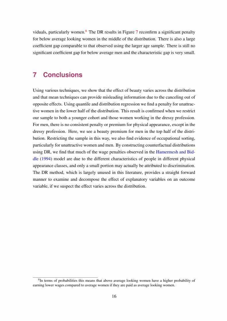
ket characteristics. If sorting occurs, individuals with less desirable physical appearancecharacteristics but higher other labor market attributes and those with desirable physicalappearance characteristics but lower other labor market attributes can be expected to sortinto "dressy" professions. If this occurs, we expect the characteristics gap to be muted.Whether sorting occurs or not, we expect a higher coefficient gap in the dressy profes-sion. In line with our results from the QR framework, we find evidence of occupationalsorting, particularly for below average looking individuals. The model for all professionscombined in Figure 2 and 3 shows a large characteristic effect for both men and women,indicating that average looking people have more desirable labor market characteristicson average. Restricting the sample to those in the dressy profession (Figures 4 and 5), wesee that there is no characteristic effect for men and a much smaller one for women, in-dicating that one of two things is happening. Either, there are relatively more ill qualifiedaverage looking people or highly qualified below average looking people. Whichever isthe case, there is distinct evidence of occupational sorting.

The coefficient effect for below average looking women in the dressy profession is higher,at around 7− 12ppt. There is also a penalty of 5− 9ppt for above average women in thelower quartile group. For men, we find a premium of 5ppt for being unattractive at thevery top of the wage distribution and a premium of 5− 7ppt for being attractive in the tophalf of the distribution.

6.2 A younger cohort

We also perform further analysis by restricting the sample to young (25-45 year olds)people, whose physical appearance may be more important in the labor market. A pre-liminary QR analysis (results available upon request) reconfirms a (stronger) penalty forbelow average looking young women in the middle of the distribution and shows a penaltyfor being above average looking only for the top of the female wage distribution. For men,QR shows a new penalty for above average looking younger men towards the top of thewage distribution. The difficulty with the QR results is that we do not know the wage rateat which these penalties occur and whether the results are comparable to the overall sam-ple. The DR results make this task much easier as individuals are compared at wage ratesrather than quantile groups, which can change by subgroup. Figure 6 shows no evidenceof a significant premium or penalty for being attractive for either men or women in thisgroup. It does show a large characteristic gap indicating that younger average lookingindividuals have better wage enhancing characteristics than above average looking indi-

15

viduals, particularly women.8 The DR results in Figure 7 reconfirm a significant penaltyfor below average looking women in the middle of the distribution. There is also a largecoefficient gap comparable to that observed using the larger age sample. There is still nosignificant coefficient gap for below average men and the characteristic gap is very small.

7 Conclusions

Using various techniques, we show that the effect of beauty varies across the distributionand that mean techniques can provide misleading information due to the canceling out ofopposite effects. Using quantile and distribution regression we find a penalty for unattrac-tive women in the lower half of the distribution. This result is confirmed when we restrictour sample to both a younger cohort and those women working in the dressy profession.For men, there is no consistent penalty or premium for physical appearance, except in thedressy profession. Here, we see a beauty premium for men in the top half of the distri-bution. Restricting the sample in this way, we also find evidence of occupational sorting,particularly for unattractive women and men. By constructing counterfactual distributionsusing DR, we find that much of the wage penalties observed in the Hamermesh and Bid-dle (1994) model are due to the different characteristics of people in different physicalappearance classes, and only a small portion may actually be attributed to discrimination.The DR method, which is largely unused in this literature, provides a straight forwardmanner to examine and decompose the effect of explanatory variables on an outcomevariable, if we suspect the effect varies across the distribution.

8In terms of probabilities this means that above average looking women have a higher probability ofearning lower wages compared to average women if they are paid as average looking women.

16

References

Averett, S. and Korenman, S. (1996). The Economic Reality of The Beauty Myth. Journal

of Human Resources, 31(2):304 – 330.

Barro, R. (1998). So You Want to Hire the Beautiful. Well, Why Not? Business Week. 3

Biddle, J. E. and Hamermesh, D. S. (1998). Beauty, Productivity, and Discrimination:Lawyers’ Looks and Lucre. Journal of Labor Economics, 16(1):172–201. 1, 2

Blinder, A. S. (1973). Wage discrimination: Reduced form and structural estimates. The

Journal of Human Resources, 8(4):pp. 436–455. 6

Bonjour, D. and Gerfin, M. (2001). The unequal distribution of unequal pay - An empiri-cal analysis of the gender wage gap in Switzerland. Empirical Economics, 26(2):407–427. 1

Buchinsky, M. (1998). The dynamics of changes in the female wage distribution in theUSA: a quantile regression approach. Journal of Applied Econometrics, 13(1):1–30. 5

Chernozhukov, V., Fernandez-Val, I., and Melly, B. (2009). Inference on counterfactualdistributions. CeMMAP working papers CWP09/09, Centre for Microdata Methodsand Practice, Institute for Fiscal Studies. 6

Foresi, S. and Peracchi, F. (1995). The Conditional Distribution of Excess Returns: AnEmpirical Analysis. Journal of the American Statistical Association, 90(430):pp. 451–466. 3, 6

Frieze, I. H., Olson, J. E., and Russell, J. (1991). Attractiveness and Income for Men andWomen in Management. Journal of Applied Social Psychology, 21(13):1039–1057. 2

Greve, J. (2007). Obesity and Labor Market Outcomes: New Danish Evidence. Work-ing Papers 07-13, University of Aarhus, Aarhus School of Business, Department ofEconomics.

Hamermesh, D. S. and Biddle, J. E. (1994). Beauty and the labor market. American

Economic Review, 84(5):1174–94. 1, 2, 3, 12, 16

Hamermesh, D. S., Meng, X., and Zhang, J. (2002). Dress for success–does primpingpay? Labour Economics, 9(3):361–373. 1, 2

Harper, B. (2000). Beauty, Stature and the Labour Market: A British Cohort Study.Oxford Bulletin of Economics and Statistics, 62:771–800. 1, 2

17

Heckman, J. J. (1979). Sample selection bias as a specification error. Econometrica,47(1):153–61. 4

Hildebrand, V. A. and Van Kerm, P. (2010). Body size and wages in Europe: A semi-parametric analysis. Social and Economic Dimensions of an Aging Population Re-search Papers 269, McMaster University.

Huber, M. and Melly, B. (2011). Quantile regression in the presence of sample selection.Economics Working Paper Series 1109, University of St. Gallen, School of Economicsand Political Science. 5

Jackson, L. (1992). Physical attractiveness: A sociocultural perspective. New York:Guilford. 2

Koenker, R. W. and Bassett, Gilbert, J. (1978). Regression quantiles. Econometrica,46(1):33–50. 5

Mathä, T. Y., Porpiglia, A., and Sierminska, E. (2011). The immigrant/native wealth gapin germany, italy and luxembourg. Working Paper Series 1302, European Central Bank.12

Mobius, M. M. and Rosenblat, T. S. (2006). Why beauty matters. American Economic

Review, 96(1)(5):222–35. 1, 2

Mocan, N. and Tekin, E. (2010). Ugly criminals. The Review of Economics and Statistics,Vol. 92, No. 1:Pages 15–30. 3

Oaxaca, R. (1973). Male-female wage differentials in urban labor markets. International

Economic Review, 14(3):693–709. 6

Register, C. A. and Williams, D. R. (1990). Wage effects of obesity among young workers.Social Science Quarterly, 71(1):130 – 141.

Sen, A., Voia, M.-C., and Woolley, F. R. (2010). Hot or not: How appearance affectsearnings and productivity in academia. Carleton Economic Papers 10-07, CarletonUniversity, Department of Economics. 1, 2

18

8 Tables and Figures

19

Table 1: A comparison of beauty ranks and importance of beauty means between womenand men and by occupation.

Panel A Women Men diffShare in each category:above 0.317 0.343 -0.025average 0.409 0.394 0.016below 0.273 0.264 0.009

Perceived importance of beauty by:all 1.970 1.834 0.135∗∗∗

above 2.022 1.894 0.129∗∗∗

average 1.925 1.821 0.105∗∗∗

under 1.974 1.775 0.198∗∗∗

Dressy:above 2.099 1.936 0.163∗∗∗

average 1.975 1.828 0.147∗∗∗

below 2.014 1.809 0.205∗∗∗

Non-dressy:above 1.809 1.836 -0.027average 1.691 1.807 -0.116below 1.890 1.742 0.148∗

Panel B Non-dressy Dressy diffPerceived importance of beauty:All 1.799 1.939 -0.140∗∗∗

Women 1.804 2.023 -0.219∗∗∗

Men 1.797 1.861 -0.064∗

Beauty ranks:All 2.015 2.091 -0.076∗∗∗

Women 1.982 2.065 -0.083∗

Men 2.029 2.115 -0.085∗∗

Source: 2007 PSELL3; t statistics in parentheses * p<0.1 ** p<0.05 *** p<0.01Note: Beauty scale: 1 - below average; 2 - average; 3 - above average.

20

Table 2: Select wage differences statistics for various beauty categories (in Euros).

Above Average diffAll 15.052 16.789 -1.736∗∗∗

Women 13.829 16.077 -2.248∗∗∗

Men 15.873 17.325 -1.452∗∗∗

Average Under diffAll 16.789 15.565 1.223∗∗

Women 16.077 14.686 1.390Men 17.325 16.224 1.101∗

Above Under diffAll 15.052 15.565 -0.513Women 13.829 14.686 -0.858Men 15.873 16.224 -0.351Source: 2007 PSELL3; t statistics in parentheses * p<0.1 ** p<0.05 *** p<0.01

21

Table 3: Select wage differences statistics for various beauty categories (in Euros).

Above Average diffWomen: Dressy 15.843 17.720 -1.877∗∗∗

Men: Dressy 19.995 20.923 -0.928Women: Non-dressy 8.312 8.945 -0.633Men: Non-dressy 10.313 10.932 -0.620

Average Under diffWomen: Dressy 17.720 17.366 0.354Men: Dressy 20.923 21.283 -0.360Women: Non-dressy 8.945 9.174 -0.229Men: Non-dressy 10.932 11.287 -0.354

Above Under diffWomen: Dressy 15.843 17.366 -1.524Men: Dressy 19.995 21.283 -1.288Women: Non-dressy 8.312 9.174 -0.862Men: Non-dressy 10.313 11.287 -0.974∗∗∗

Source: 2007 PSELL3; t statistics in parentheses * p<0.1 ** p<0.05 *** p<0.01

22

Tabl

e4:

OL

S,se

lect

ion

mod

elan

dqu

antil

ere

gres

sion

s(w

omen

).(1

)(2

)(3

)(4

)(5

)(6

)(7

)(8

)

OL

Sln

hrw

ork

q10

q25

q50

q75

q90

unde

r_av

g-0

.07

-0.0

7-0

.04

-0.0

8**

-0.0

8**

-0.0

5-0

.10

unde

r*dr

essy

-0.0

2-0

.02

-0.0

5-0

.03

0.00

0.00

0.02

abov

e_av

g-0

.10*

*-0

.10*

*-0

.11

-0.1

1***

-0.1

0**

-0.0

7-0

.13*

abov

e*dr

essy

0.09

0.09

0.06

0.05

0.09

0.09

0.11

dres

sy0.

15**

*0.

15**

*0.

110.

12**

*0.

17**

*0.

19**

*0.

19**

mar

ried

0.00

-0.0

0-0

.52*

**0.

040.

040.

030.

020.

04lt

high

scho

ol-0

.14*

**-0

.14*

**-0

.06

-0.1

0***

-0.1

1***

-0.1

8***

-0.2

1***

colle

ge0.

42**

*0.

42**

*0.

27**

*0.

36**

*0.

39**

*0.

38**

*0.

38**

*ex

peri

ence

0.02

***

0.02

***

0.02

***

0.02

***

0.02

***

0.03

***

0.02

***

expe

rien

ce2

-0.0

0*-0

.00*

-0.0

0*-0

.00*

*-0

.00

-0.0

0**

-0.0

0pa

rt-t

ime

0.16

***

0.16

***

-0.0

00.

020.

11**

*0.

23**

*0.

24**

*bi

gco

mpa

ny0.

13**

*0.

13**

*0.

10**

*0.

11**

*0.

11**

*0.

11**

*0.

12**

*te

mpo

rary

-0.1

3*-0

.13*

-0.3

0***

-0.2

1***

-0.1

6***

-0.0

8-0

.03

civi

lser

vant

0.34

***

0.34

***

0.46

***

0.40

***

0.40

***

0.34

***

0.38

***

Port

uges

e-0

.16*

**-0

.15*

**0.

57**

*-0

.18*

**-0

.22*

**-0

.22*

**-0

.25*

**-0

.27*

**ot

hern

on-n

ativ

e-0

.14*

**-0

.14*

**0.

11-0

.17*

**-0

.16*

**-0

.15*

**-0

.11*

**-0

.07*

bad

heal

th0.

040.

03-0

.47*

*-0

.10

-0.0

7-0

.10

0.01

-0.0

2ag

e0.

34**

*ag

e2-0

.42*

**N

o.ch

ildre

n-0

.27*

**ch

ild-0

.03

prox

y-0

.04

Con

stan

t2.

24**

*2.

22**

*-5

.48*

**2.

03**

*2.

18**

*2.

27**

*2.

38**

*2.

56**

*λ

0.02

ρ0.

05σ

0.36

***

Wal

dte

st(χ

2)

0.22

Pseu

do-R

20.

570,

218

0,33

50,

410

0,41

40,

413

Obs

erva

tions

1,54

32,

903

2,90

31,

543

1,54

31,

543

1,54

31,

543

Sour

ce:2

007

PSE

LL

3;R

obus

tsta

ndar

der

rors

used

.Boo

tstr

appe

dst

anda

rder

rors

forq

uant

ilere

gres

sion

s(2

00re

ps).

tsta

tistic

sin

pare

nthe

ses

*p<

0.1

**p<

0.05

***

p<0.

01N

ote:

We

drop

obse

rvat

ions

with

wag

e=0

23

Tabl

e5:

OL

S,se

lect

ion

mod

elan

dqu

antil

ere

gres

sion

s(m

en).

(1)

(2)

(3)

(4)

(5)

(6)

(7)

(8)

OL

Sln

hrw

ork

q10

q25

q50

q75

q90

unde

r_av

g0.

030.

030.

020.

03-0

.01

-0.0

1-0

.03

unde

r*dr

essy

-0.0

2-0

.02

-0.0

8-0

.03

0.07

*0.

060.

07ab

ove_

avg

-0.0

1-0

.01

-0.0

0-0

.00

-0.0

1-0

.04

-0.0

1ab

ove*

dres

sy0.

030.

03-0

.04

-0.0

10.

000.

07*

0.02

dres

sy0.

21**

*0.

21**

*0.

070.

10**

*0.

15**

*0.

19**

*0.

23**

*m

arri

ed0.

06*

0.06

*0.

180.

09**

*0.

08**

*0.

09**

*0.

08**

*0.

09**

*lt

high

scho

ol-0

.19*

**-0

.19*

**-0

.05*

-0.1

1***

-0.1

4***

-0.1

5***

-0.1

9***

colle

ge0.

36**

*0.

36**

*0.

43**

*0.

43**

*0.

45**

*0.

39**

*0.

42**

*ex

peri

ence

0.03

***

0.04

***

0.02

***

0.02

***

0.03

***

0.03

***

0.03

***

expe

rien

ce2

-0.0

0***

-0.0

0***

-0.0

0-0

.00*

**-0

.00*

**-0

.00*

**-0

.00*

**pa

rt-t

ime

0.30

***

0.30

***

-0.3

5*0.

090.

23**

0.43

***

0.54

***

big

com

pany

0.16

***

0.16

***

0.12

***

0.13

***

0.10

***

0.10

***

0.05

*te

mpo

rary

-0.1

9***

-0.1

9***

-0.2

4***

-0.1

9***

-0.0

9**

-0.1

0***

-0.0

9*ci

vils

erva

nt0.

27**

*0.

27**

*0.

45**

*0.

36**

*0.

26**

*0.

21**

*0.

17**

*Po

rtug

ese

-0.2

1***

-0.2

1***

0.49

***

-0.1

9***

-0.2

5***

-0.2

5***

-0.2

7***

-0.2

7***

othe

rnon

-nat

ive

-0.1

2***

-0.1

2***

0.00

-0.1

8***

-0.2

0***

-0.2

0***

-0.1

0***

-0.0

4ba

dhe

alth

-0.1

1*-0

.12

-1.8

4***

-0.1

1-0

.11*

-0.1

9***

-0.1

9***

-0.2

3***

age

0.49

***

age2

-0.6

2***

noch

-0.0

5ch

ild0.

19pr

oxy

0.14

Con

stan

t2.

24**

*2.

24**

*-8

.05*

**2.

08**

*2.

21**

*2.

34**

*2.

47**

*2.

69**

*λ

0.01

ρ0.

18σ

-0.3

3***

Wal

dte

st(χ

2)

0.01

Pseu

do-R

20.

630.

257

0.37

60.

443

0.45

40.

452

Obs

erva

tions

2,12

72,

782

2,78

22,

127

2,12

72,

127

2,12

72,

127

Sour

ce:2

007

PSE

LL

3;R

obus

tsta

ndar

der

rors

used

.Boo

tstr

appe

dst

anda

rder

rors

forq

uant

ilere

gres

sion

s(2

00re

ps).

tsta

tistic

sin

pare

nthe

ses

*p<

0.1

**p<

0.05

***

p<0.

01N

ote:

We

drop

obse

rvat

ions

with

wag

e=0

24

Figure 1 Cumulative distribution function and counterfactual CDF for above average andaverage women.

Source: 2007 PSELL3Note: Wage distribution for reported looks: ABab- above average; AV av- average;AV ab- above average paid as averageABab− AV ab coefficient gap; AV ab− AV av characteristic gap

25

Figure 2 Coefficient and characteristics gaps for above average vs. average women andmen.

Source: 2007 PSELL3Note: Wage distribution for reported looks: ABab- above average; AV av- average;AV ab- above average paid as average. Gap > 0 indicates a higher probability of lowerwages for the above average group. ABab− AV ab coefficient gap; AV ab− AV avcharacteristic gap 26

Figure 3 Coefficient and characteristics gaps for under average vs. average women andmen.

Source: 2007 PSELL3Note: Wage distribution for reported looks: UNun- under average; AV av- average;AV un- under average paid as average. Gap > 0 indicates a higher probability of lowerwages for the under average group. UNun− AV un - coefficient gap; AV un− AV av -characteristic gap 27

Figure 4 Coefficient and characteristics gaps for above average vs. average women andmen in the dressy profession.

Source: 2007 PSELL3Note:Wage distribution for reported looks: ABab- above average; AV av- average;AV ab- above average paid as average. Gap > 0 indicates a higher probability of lowerwages for the above average group. ABab− AV ab coefficient gap; AV ab− AV avcharacteristic gap

28

Figure 5 Coefficient and characteristics gaps for under average vs. average women andmen in the dressy profession.

Source: 2007 PSELL3Note: Wage distribution for reported looks: UNun- under average; AV av- average;AV un- under average paid as average. Gap > 0 indicates a higher probability of lowerwages for the under average group. UNun− AV un coefficient gap; AV un− AV avcharacteristic gap

29

Figure 6 Coefficient and characteristics gaps for above average vs. average women andmen between 25-45 years of age.

Source: 2007 PSELL3Note: Wage distribution for reported looks: ABab- above average; AV av- average;AV ab- above average paid as average. Gap > 0 indicates a higher probability of lowerwages for the above average group. ABab− AV ab coefficient gap; AV ab− AV avcharacteristic gap

30

Figure 7 Coefficient and characteristics gaps for under average vs. average women andmen between 25-45 years of age.

Source: 2007 PSELL3Note: Wage distribution for reported looks: UNun- under average; AV av- average;AV un- under average paid as average. Gap > 0 indicates a higher probability of lowerwages for the under average group. UNun− AV un coefficient gap; AV un− AV avcharacteristic gap

31

Figure A1 Self-assessed beauty by occupation (in percentages).

Source: 2007 PSELL3

32

Figure A2 Goodness of fit of the distribution regressions.

Source: 2007 PSELL3

33

Table A1: Explanatory variables used for estimation.married 1 if married

lt high school 1 if highest education received is first cycle of highschoolcollege 1 if highest education received is third level

experience self-reported number of years workingpart-time 1 if work < 30hours per week

big company 1 if > 50 employees at workplacetemporary 1 if temporary contract

civil servant 1 if public sector employeePortugese 1 if portuguese nationality

other-non-native 1 if nationality other than portuguese/luxembourgishbad health 1 if classify health as bad/very bad

age age in yearsno. children number of children the individual has

child 1 if the individual has childrenproxy 1 if the individual did not answer the questionnaire themselves

below_avg self-reported physical appearance of 1-5 out of 10above_avg self reported physical appearance of 8-10 out of 10

dressy 1 if the individual works in a "dressy" professionSource: 2007 PSELL3/EU-SILC

34

Table A2: Select statistics for above average, average and under average beauty (women)(1) (2) (3) (4) (5)

Above Average Under (1)-(2) diff (2)-(3) diffage 36.409 37.367 38.327 -0.958 -0.960married 0.549 0.556 0.548 -0.007 0.008single 0.309 0.317 0.302 -0.008 0.016separated 0.142 0.127 0.151 0.015 -0.024no. children 1.210 1.150 1.357 0.059 -0.207∗∗∗

children (0/1) 0.643 0.641 0.682 0.002 -0.041lt high school 0.371 0.249 0.422 0.122∗∗∗ -0.173∗∗∗

high school 0.285 0.302 0.332 -0.016 -0.030college 0.333 0.437 0.232 -0.103∗∗∗ 0.205∗∗∗

work experience 14.607 14.980 16.599 -0.373 -1.619∗∗

full-time 0.727 0.669 0.664 0.058∗∗ 0.005part-time 0.323 0.390 0.392 -0.067∗∗ -0.002big company 0.397 0.497 0.455 -0.100∗∗∗ 0.042temporary 0.126 0.093 0.107 0.033∗ -0.014civil servant 0.192 0.257 0.206 -0.065∗∗∗ 0.050∗

native 0.355 0.401 0.404 -0.046 -0.003Portugese 0.242 0.166 0.346 0.076∗∗∗ -0.180∗∗∗

other non-native 0.403 0.433 0.251 -0.030 0.183∗∗∗

bad health 0.042 0.023 0.044 0.019∗ -0.021∗

great health 0.417 0.409 0.288 0.008 0.121∗∗∗

Occupation type: Dressy 0.733 0.813 0.673 -0.080∗∗∗ 0.140∗∗∗

Observations 501 646 431 Total 1578Source: 2007 PSELL3; t statistics in parentheses * p<0.1 ** p<0.05 *** p<0.01

35

Table A3: Select statistics for above average and average beauty (men)(1) (2) (3) (4) (5)

Above Average Under (1)-(2) diff (2)-(3) diffage 37.193 38.029 39.400 -0.836 -1.371∗∗

married 0.609 0.597 0.637 0.012 -0.040single 0.321 0.326 0.259 -0.005 0.067∗∗∗

separated 0.070 0.077 0.104 -0.007 –0.027∗

no. children 1.277 1.191 1.428 0.086 –0.237∗∗∗

children (0/1) 0.641 0.608 0.697 0.033 -0.089∗∗∗

lt high school 0.347 0.307 0.440 0.040∗ -0.133∗∗∗

high school 0.352 0.315 0.317 0.037 -.002college 0.297 0.373 0.231 -0.076∗∗∗ 0.142∗∗∗

work experience 17.525 17.809 20.880 -0.284 -3.071∗∗∗

full-time 0.983 0.977 0.977 0.006 -0.001part-time 0.031 0.040 0.037 -0.009 0.003big company 0.499 0.590 0.581 -0.090∗∗∗ 0.009temporary 0.116 0.086 0.096 0.030∗∗ -0.009civil servant 0.171 0.210 0.150 -0.038∗ 0.060∗∗∗

native 0.348 0.395 0.350 -0.047∗ 0.046∗

Portugese 0.285 0.217 0.374 0.068∗∗∗ -0.157∗∗∗

other non-native 0.367 0.388 0.277 -0.021 0.112∗∗∗

bad health 0.013 0.017 0.050 -0.004 -0.033∗∗∗

great health 0.444 0.407 0.306 0.038 0.101∗∗∗

Occupation type: Dressy 0.574 0.640 0.494 -0.066∗∗∗ 0.146∗∗∗

Observations 747 858 575 Total 2180Source: 2007 PSELL3; t statistics in parentheses * p<0.1 ** p<0.05 *** p<0.01

36

3, avenue de la FonteL-4364 Esch-sur-AlzetteTél.: +352 58.58.55-801www.ceps.lu