Robert M. ManningGlenn Research Center, Cleveland, Ohio

Beamed-Energy Propulsion (BEP): Considerations for Beaming High Energy-Density Electromagnetic Waves Through the Atmosphere

NASA/TM—2015-218726

May 2015

NASA STI Program . . . in Profile

Since its founding, NASA has been dedicated to the advancement of aeronautics and space science. The NASA Scientific and Technical Information (STI) Program plays a key part in helping NASA maintain this important role.

The NASA STI Program operates under the auspices of the Agency Chief Information Officer. It collects, organizes, provides for archiving, and disseminates NASA’s STI. The NASA STI Program provides access to the NASA Technical Report Server—Registered (NTRS Reg) and NASA Technical Report Server—Public (NTRS) thus providing one of the largest collections of aeronautical and space science STI in the world. Results are published in both non-NASA channels and by NASA in the NASA STI Report Series, which includes the following report types: • TECHNICAL PUBLICATION. Reports of

completed research or a major significant phase of research that present the results of NASA programs and include extensive data or theoretical analysis. Includes compilations of significant scientific and technical data and information deemed to be of continuing reference value. NASA counter-part of peer-reviewed formal professional papers, but has less stringent limitations on manuscript length and extent of graphic presentations.

• TECHNICAL MEMORANDUM. Scientific

and technical findings that are preliminary or of specialized interest, e.g., “quick-release” reports, working papers, and bibliographies that contain minimal annotation. Does not contain extensive analysis.

• CONTRACTOR REPORT. Scientific and technical findings by NASA-sponsored contractors and grantees.

• CONFERENCE PUBLICATION. Collected papers from scientific and technical conferences, symposia, seminars, or other meetings sponsored or co-sponsored by NASA.

• SPECIAL PUBLICATION. Scientific,

technical, or historical information from NASA programs, projects, and missions, often concerned with subjects having substantial public interest.

• TECHNICAL TRANSLATION. English-

language translations of foreign scientific and technical material pertinent to NASA’s mission.

For more information about the NASA STI program, see the following:

• Access the NASA STI program home page at http://www.sti.nasa.gov

• E-mail your question to help@sti.nasa.gov • Fax your question to the NASA STI

Information Desk at 757-864-6500

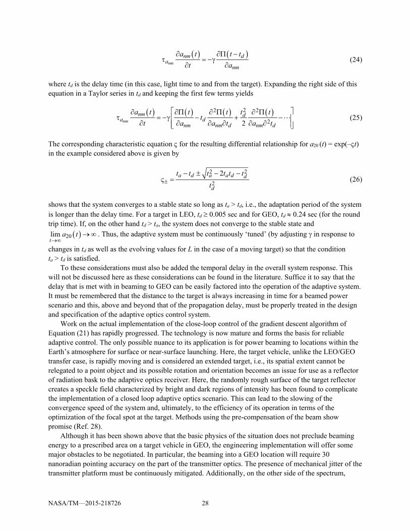
• Telephone the NASA STI Information Desk at 757-864-9658 • Write to:

NASA STI Program Mail Stop 148 NASA Langley Research Center Hampton, VA 23681-2199

Robert M. ManningGlenn Research Center, Cleveland, Ohio

Beamed-Energy Propulsion (BEP): Considerations for Beaming High Energy-Density Electromagnetic Waves Through the Atmosphere

NASA/TM—2015-218726

May 2015

National Aeronautics andSpace Administration

Glenn Research Center Cleveland, Ohio 44135

Available from

Level of Review: This material has been technically reviewed by technical management.

NASA STI ProgramMail Stop 148NASA Langley Research CenterHampton, VA 23681-2199

National Technical Information Service5285 Port Royal RoadSpringfield, VA 22161

703-605-6000

This report is available in electronic form at http://www.sti.nasa.gov/ and http://ntrs.nasa.gov/

Beamed-Energy Propulsion (BEP): Considerations for Beaming High Energy-Density Electromagnetic

Waves Through the Atmosphere

Robert M. Manning National Aeronautics and Space Administration

Glenn Research Center Cleveland, Ohio 44135

Preface A study to determine the feasibility of employing beamed electromagnetic energy for vehicle

propulsion within and outside the Earth’s atmosphere was co-funded by NASA and the Defense Advanced Research Projects Agency that began in June 2010 and culminated in a Summary Presentation in April 2011. A detailed report entitled “Beamed-Energy Propulsion (BEP) Study” appeared in February 2012 as NASA/TM—2012-217014. Of the very many nuances of this subject that were addressed in this report, the effects of transferring the required high energy-density electromagnetic fields through the atmosphere were discussed. However, due to the limitations of the length of the report, only a summary of the results of the detailed analyses were able to be included. It is the intent of the present work to make available the complete analytical modeling work that was done for the BEP project with regard to electromagnetic wave propagation issues. In particular, the present technical memorandum contains two documents that were prepared in 2011. The first one, entitled “Effects of Beaming Energy Through the Atmosphere” contains an overview of the analysis of the nonlinear problem inherent with the transfer of large amounts of energy through the atmosphere that gives rise to thermally-induced changes in the refractive index; application is then made to specific beamed propulsion scenarios. A brief portion of this report appeared as Appendix G of the 2012 Technical Memorandum. The second report, entitled “An Analytical Assessment of the Thermal Blooming Effects on the Propagation of Optical and Millimeter-Wave Focused Beam Waves For Power Beaming Applications” was written in October 2010 (not previously published), provides a more detailed treatment of the propagation problem and its effect on the overall characteristics of the beam such as its deflection as well as its radius. Comparisons are then made for power beaming using the disparate electromagnetic wavelengths of 1.06 µm and 2.0 mm.

NASA/TM—2015-218726 iii

Contents Preface ......................................................................................................................................................... iii Chapter 1.—Effects of Beaming Energy Through the Atmosphere ............................................................. 1

1.1 Executive Summary ...................................................................................................................... 1 1.2 Introduction ................................................................................................................................... 1 1.3 The Deleterious Atmospheric Propagation Mechanisms at High Energies .................................. 3

1.3.1 Ionization and Electrical Breakdown ................................................................................ 3 1.3.2 Induced Molecular Polarization—The Kerr Effect ........................................................... 3 1.3.3 Induced Heating of the Atmosphere—Thermal Nonlinearities and “Thermal

Blooming” ......................................................................................................................... 4 1.3.4 Atmospheric Aerosols ....................................................................................................... 4 1.3.5 Atmospheric Turbulence ................................................................................................... 5

1.4 Modeling the Effects of Atmospheric Thermal Nonlinearities on Beamed Energy Propulsion and the Required Level of Their Mitigation ............................................................... 6 1.4.1 A Quick Overview of the Model and the Description of Beam Behavior at a

Target in LEO and GEO due to Atmospheric Thermal Nonlinearities ............................. 7 1.4.2 Application of the Foregoing to the Calculation of Beam Spread and Deflection

due to Atmospheric Thermal Nonlinearities for Power Beaming to LEO and GEO................................................................................................................................... 8

1.4.3 Phase Compensation of the Effects of Atmospheric Thermal Nonlinearities ................. 13 1.4.4 Using the Propagation Model for the Analysis of Millimeter Wave Beaming

Within the Earth’s Atmosphere ....................................................................................... 18 1.4.5 A Tool for the Quick Assessment of Nonlinear Thermal Effects on Power

Beaming .......................................................................................................................... 25 1.5 Dynamics of Adaptive Phase Compensation for Power-Beaming Applications ........................ 26 1.6 Experiments Assessing the Compensation of Thermal Nonlinearities of High Power

Beams in the Atmosphere ........................................................................................................... 29 1.7 Conclusions and Recommendations ........................................................................................... 29

Appendix A.—The Derivation of the Fundamental Nonlinear Propagation Equations for High Energy Transmission Through the Atmosphere and the Associated Critical Powers ....................................... 31 A.1 The Critical Power for the Atmospheric the Kerr Effect ............................................................ 33 A.2 The Critical Power for Atmospheric Thermal Effects ................................................................ 34

A.2.1 Continuous Wave Source ................................................................................................ 34 A.2.2 Pulsed Source .................................................................................................................. 36

A.3 Conclusion .................................................................................................................................. 37 References ............................................................................................................................................ 38

Chapter 2.—An Analytical Assessment of the Thermal Blooming Effects on the Propagation of Optical And Millimeter-Wave Focused Beam Waves For Power Beaming Applications................................ 41 2.1 Introduction ................................................................................................................................. 41

2.1.1 A Simple Analytical Model for Beam Broadening and Displacement ........................... 42 2.1.2 Application of the Foregoing to Millimeter and Optical Wavelength Power

Beaming .......................................................................................................................... 46 References ............................................................................................................................................ 48

NASA/TM—2015-218726 v

Chapter 1.—Effects of Beaming Energy Through the Atmosphere 1.1 Executive Summary

Power beaming the large amounts of energy through the atmosphere that is required for propulsion either within the atmosphere or in transferring payloads from LEO to GEO will be met with the extremely deleterious effects of the thermal nonlinearities induced by atmospheric heating from beam power absorption. The resulting phenomena, collectively called thermal blooming, will be the source of two major effects, i.e., beam steering away from the intended target vehicle as well as beam broadening which will make the beam larger at the target than intended. Both of these effects have been modeled and are shown here to be remedied by the use of high order (10th order Hermite) phase compensation at the transmitter. Although it has been shown that these perturbations can be mitigated in principle, there may remain many engineering obstacles that must be overcome, such as elimination of mechanical jitter of the transmitter platform, etc., during beam propagation. However, there is nothing in the prevailing physics of the situation that would preclude power beaming through the atmosphere as discussed in this report.

It is important to begin to capture the prevailing effects and overall system operation using a scaled atmospheric experiment that would simulate the realistic environment in which an adaptive optics system must operate, from the variable wind velocity up to the mechanical jitter of the transmitter platform. It is recommended that, due to the immediate availability of high power sources, scaled atmospheric experiments be implemented (tailored after the Scaled Atmospheric Blooming Experiments (SABLE) Project by Lincoln Laboratory in the early 1990s) in which the operation of a closed-loop millimeter wave adaptive optics algorithm is assessed in the presence of a moving extended target. Additionally, this experimental scenario can also be used to address the issue related to the possibility of air ionization, and subsequent breakdown, across the apertures of the combined millimeter wave gyrotron sources as discussed elsewhere in this report.

Finally, there is the need to look at various general beam wave profiles such as hypergaussian as well as fractional charge (in the topological sense) Laguerre-Gaussian beam waves that show great promise in their ability to be robust with respect to atmospheric nonlinearities. However, it is important that the modeling effort be kept to the level of yielding analytical results, rather than requiring numerical evaluation, so as to capture all the nuances of the physics involved and, at the same time, provide a tool for overall system evaluation as well as the design of adaptive optics algorithms. Finally, the model should be incorporated into a trajectory analysis program so a cadre of launch geometries can be evaluated from the point of view of atmospheric thermal nonlinearities.

1.2 Introduction

When delivering large amounts of power through the Earth’s atmosphere via millimeter or infrared ‘beams’ (i.e., laser beams or beams formed at the output of a millimeter wave antenna system), many propagation mechanisms must be addressed that may be potentially deleterious such power transmission. The most obvious one is the ever-present random variation of the atmospheric refractive index due to local temperature variations known as ‘turbulence’. This naturally occurring phenomena is driven by thermal convection of heat from the Earth’s surface; once the resulting air motion exceeds a critical value of velocity, laminar flow essentially evolves into turbulent flow and fluctuations in the temperature distribution becomes statistically random (Ref. 1). These temperature fluctuations then act directly on the prevailing refractive index, thus rendering the refractive index a random quantity. These refractive index variations randomly focus and defocus the intervening electromagnetic wave field. Thus, the atmosphere

NASA/TM—2015-218726 1

can be considered to be composed of ‘lenses’ of random focusing and defocusing characteristics that, due to the gross atmospheric motion due to wind, move across the beam. This gives rise to many beam quality variations; the major ones being beam broadening and beam steering. The statistical analysis and modeling of this type of atmospheric propagation as a long and rich history and has resulted in analytical descriptions for the impact of turbulence on the operation of systems relying on such beam propagation. Many models and descriptions exist for the ‘engineering analysis’ of the operation of transmission systems that rely on the propagation of electromagnetic beam propagation in the atmosphere (for a good recent treatment, see Ref. 2 and the references therein).

The scenario discussed above may be considered as ‘passive’ electromagnetic wave propagation, i.e., the wave field moves through an atmosphere the refractive index of which is determined by other sources, not the field itself. However, as the energy density of the beam increases, absorption of the beam energy by atmospheric gas components results in local heating of the atmospheric which does indeed act directly on the refractive index causing it to decrease in value. The possibility of this situation was first advanced in 1966 (Ref. 3). This thermal change of the refractive index field then acts on the electromagnetic wave field causing it to also change, and so on. The propagation scenario now becomes an ‘active’ one, whereby the propagating field modifies the very medium it which it exists. This heating process is called ‘thermal blooming’ and substantially differs from that of the passive propagation discussed earlier (Refs. 4 and 5 (Ref. 5 contains a very comprehensive review of work and references that existed up to 1990)). Here, a ‘thermal lens’ is created within the atmosphere by the heating due to the energy density of the beam. This ‘self-action’ of the beam will not only bend the beam into regions of higher refractive index (beam steering), but convection within the atmospheric fluid will also arise which is the source of self-induced turbulent flow of the medium. The situation is further complicated when one includes the effects of atmospheric wind and aerosols and the abovementioned passive propagation effects. Defocusing and other such associated nonlinear thermal blooming distortions of the beam cross-section will then result. In extreme cases of very large energy densities, the propagating beam will essentially break up into smaller beams, or filaments, which severely constrains the amount of energy density that the beam will be able to possess as it travels through the atmosphere. Unlike the situation of passive propagation, the thermal blooming mechanism introduces nonlinearities into the analysis of the phenomena that substantially complicates a complete mathematical description. Complete analyses of these types of propagation scenarios can only be done numerically, which was a major activity within the United States and Russia in the late 1980s. Other than the usual ‘order-of-magnitude’ estimates using the equations of fluid mechanics and wave propagation, only numerical modeling of the effects of atmospheric thermal nonlinearities abound in the literature. Analytical treatments appropriate for an engineering analysis of atmospheric propagation systems encountering thermal blooming have been lacking, especially those that endeavor to describe the result of adaptive correction of such nonlinear effects. This situation makes a comparative assessment of the operation of through-the-atmosphere power transmission difficult.

In order to assess the atmospheric effects on the various beamed energy propulsion scenarios considered in this report, the propagation environment of high-energy electromagnetic wave transmission within the Earth’s atmosphere will be presented. First, a brief review will be given in Section 1.3 of the major physical mechanisms that prevail in the atmosphere that will deleteriously affect energy transfer via electromagnetic beam waves. The critical power thresholds for the wavelengths of 2.0 µm (infrared) and 2.0 mm (millimeter wave) will be derived for various transmitter output aperture sizes at which these propagation mechanisms arise and must be addressed. Once this has been accomplished, Section 1.4 will present a propagation model that will be used to calculate the thermally-induced beam broadening and steering that will occur for a 2.0 µm laser beam, for a variety of aperture sizes and output powers,

NASA/TM—2015-218726 2

transmitted from the Earth’s surface to a target at distances of 800 to 35200 km. The adaptive correction to mitigate the thermal nonlinearity effects on the beam will then be considered. Of the various performance parameters that an adaptive optics system can be designed to optimize at the target, it will be the minimization of the beam radius at target that will be the optimization parameter. Section 1.5 will then dwell on the dynamics that an adaptive optics system must satisfy, particularly with regard to the control delays inherent with the propagation distances that are involved. Finally, Section 1.6 will highlight some scaled ground experiments that can be performed using available high power millimeter wave sources. In particular, the effects of using an extended target with a closed-loop adaptive optics approach can be assessed. At this same time, the possible electrical breakdown of moist air in the vicinity of the combined gyrotron outputs can be studied.

1.3 The Deleterious Atmospheric Propagation Mechanisms at High Energies

At the power densities that are required for beamed energy propulsion, several aspects of propagation within the atmosphere must be addressed that can potentially perturb the beam wave and render it unreliable for energy transfer to a small target. Once these aspects have been identified, physically understood and mathematically modeled, appropriate mitigation procedures can be specified and applied to the problem to optimize energy transfer. These propagation features and the critical power levels at which they will be seen will now be given.

1.3.1 Ionization and Electrical Breakdown When considering the transmission of high energy electromagnetic waves through the atmosphere,

the first phenomenon that is considered is air ionization and the subsequent electrical breakdown (Ref. 6, a good introduction and the original work). Within the atmosphere, this occurs via the process of cascade ionization whereby a free electron is created by multiquantum absorption by the atmospheric gas and through the inverse bremsstrahlung process, accelerates and subsequently collides with an atom. The collision produces another electron, and both accelerate, collide with other atoms, and so on. This cascading process terminates in the release of light known as electrical breakdown. At a wavelength of λ = 10.6 µm (i.e., the wavelength of high power CO2 lasers), electrical breakdown occurs at a power density of ≈ 109 W/cm2 at atmospheric pressures and densities typical of those at sea level. This intensity is reduced by two orders of magnitude by the formation of the shock front due to the explosive detonation of atmospheric aerosols. Thus, for purposes of comparison, one can choose a power density of ≈ 107 W/cm2 as the threshold for electrical breakdown within the atmosphere.

At millimeter wavelengths in the 100 to 200 GHz frequency range, electrical breakdown occurs at a smaller power density of ≈ 1010 W/m2. One can then assume the worst case of a twofold decrease in this value due to atmospheric aerosols, thus giving a threshold power density of ≈ 108 W/m2.

1.3.2 Induced Molecular Polarization—The Kerr Effect The next process that must be considered is the Kerr effect, i.e., the process whereby the permittivity

of the atmosphere, which is a function of the polarizability of the constituent gases, varies due the intense electric field of the laser beam acting to induce molecular orientation (Refs. 7 and 8). As discussed in the Appendix, the Kerr process can be described by a single differential equation, making its analysis straightforward as compared to the thermally-induced permittivity variations to be discussed in the next section. The associated relaxation times for molecular polarizability within the atmosphere are ~ 1011 sec. so in the case of pulsed laser propagation, the medium can be considered in steady state for pulse lengths larger than this value. As the brief analysis in the Appendix shows, the threshold value PcrK of beam

NASA/TM—2015-218726 3

power at which the Kerr effect is only a function of the Kerr constant and the wavelength (see Eq. (A17)); it becomes an issue as a perturbing propagation mechanism at PcrK ≈ 1.5×109 W for the wavelength of λ = 2.0 µm and PcrK ≈ 1.5×1016 W at λ = 2.0 mm. The Kerr effect serves to increase the permittivity in the location of the beam and thus results in what has become to be known as “self-focusing”, i.e., the beam tends to move into regions of larger permittivity and thus acts as if it has encountered a lens. The lens is essentially induced by the beam through the Kerr effect. This self-focusing phenomena results in a spatial instability within the beam causing a break-up of the beam into individual filaments, where each filament takes on the size which corresponds to PcrK and the associated electric field strength.

1.3.3 Induced Heating of the Atmosphere—Thermal Nonlinearities and “Thermal Blooming” The absorption of electromagnetic radiation by atmospheric gases becomes a source for the

generation of heat. At large field intensities, the resulting temperature increase also changes the atmospheric permittivity. However, unlike the Kerr effect, the permittivity decreases and the beam tends to defocus (Refs. 4, 5, 9 to 12). Additionally, one must also admit the description of the atmospheric fluid dynamic processes that are elicited due to local heating and thus incorporate the Navier-Stokes and heat transfer equations for a moving medium; the medium is in motion not only due to the Archimedean forces that appear but also due to wind which serves to remove the heat that is generated. The problem in its entirety is a severely complicated one and is usually relegated to numerical analysis applied to specific cases. However, within certain approximations, analytical results can be obtained. As shown in the Appendix, one can obtain an expression for the critical power PcrT the beam must possess above which thermally-induced propagation issues can become prominent. Due to the interplay of the several physical mechanisms that prevail in this propagation process, one must specify the prevailing wind velocity V as well as the effective radius reff of the output aperture of the beam source and the wavelength dependent absorption constant α. As given by Equation (A25), one has for V = 4.4 m/s (≈10 mi/hr), reff = 10 m and λ = 2.0 µm, for which α ≈ 4×10–6 m–1, PcrT = 16.7 W, a surprisingly small power. This is mainly due to the very large radius subtended by the beam through which the field-induced temperature increase must dissipate due to wind. For a more typical radius of reff = 0.1 m, one has PcrT ≈ 1.7 KW. At the much larger wavelength λ = 2.0 mm, one has α ≈ 2.2×10–4 m–1 giving for reff = 10 m, PcrT = 3.5×105 W.

In the case where the radiation source is pulsed with time duration of 1 µs, the threshold power becomes much higher due to the fact that the atmosphere does not have sufficient time to heat during the movement of the pulse through the atmosphere. As obtained from Equation (A31), one has for the critical power at λ = 2.0 µm, PcrP = 3.7×107 W and for λ = 2.0 mm, PcrP = 7.7×1011 W.

1.3.4 Atmospheric Aerosols The appearance of aerosols in the form of fog and clouds serve to be very efficient absorbers of

electromagnetic radiation (Refs. 13 and 14). At the energy densities that prevail for beamed energy propulsion, aerosols will essentially explosively detonate thus diminishing their absorption and scattering abilities. The dynamics of this complex process has been well studied and it has been established that, once a steady state has been established, propagation ‘channels’ will appear in the medium through which the beam can propagate (Refs. 15 and 16).

NASA/TM—2015-218726 4

1.3.5 Atmospheric Turbulence The effect of random variations of the atmospheric permittivity field due to heating of the

atmosphere, (the sources of which are solar absorption in the atmosphere and on the Earth’s surface) is independent of the beam power level for the lowest critical power thresholds derived above for the thermal blooming case. This ever-present deleterious mechanism has the most heritage in terms of study and understanding. The effects of this phenomenon on the propagation of a beam wave show themselves in terms of loss of spatial coherence, beam steering and beam broadening and are attendant with thermal blooming (Ref. 17). Of course, these characteristics are the same as seen with thermal blooming but the adaptive compensation in the case of turbulence is straightforward in that the effect being corrected is not the result of a nonlinear process.

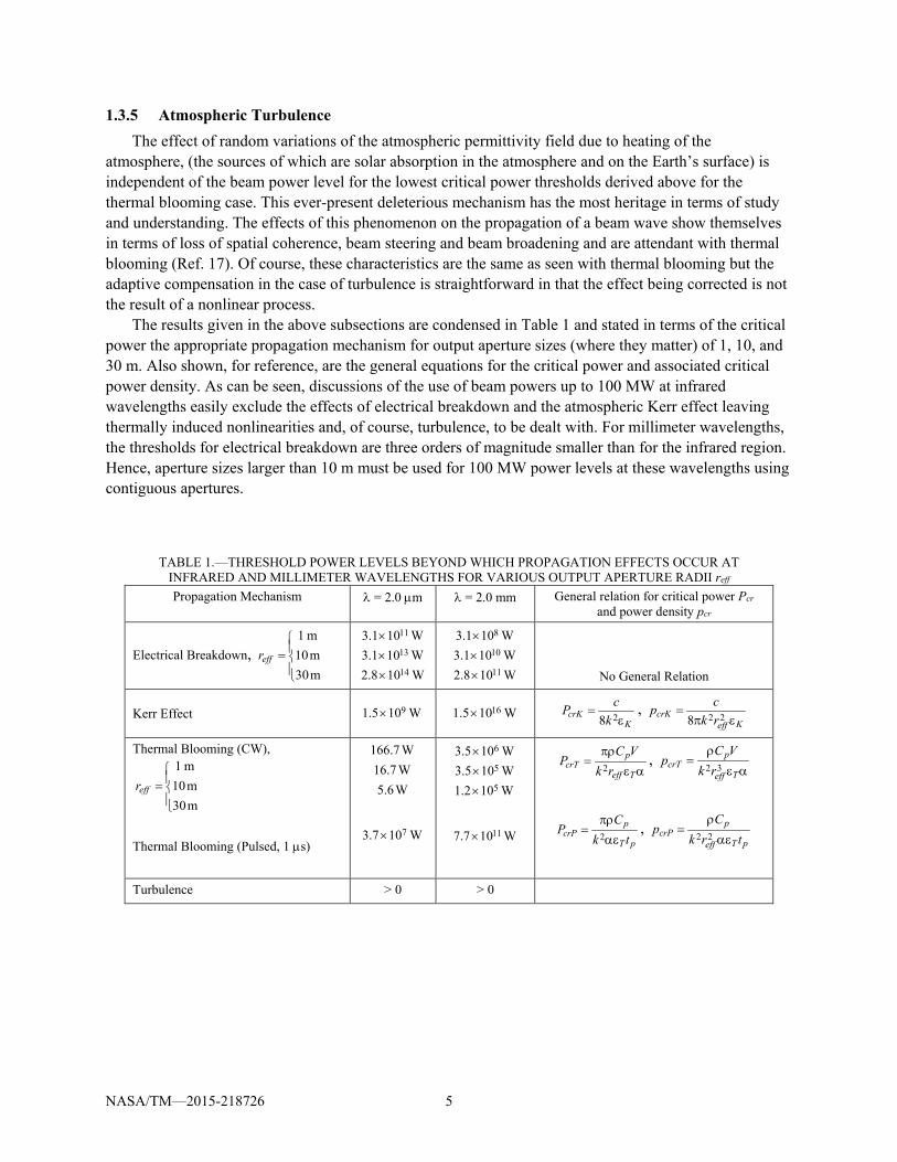
The results given in the above subsections are condensed in Table 1 and stated in terms of the critical power the appropriate propagation mechanism for output aperture sizes (where they matter) of 1, 10, and 30 m. Also shown, for reference, are the general equations for the critical power and associated critical power density. As can be seen, discussions of the use of beam powers up to 100 MW at infrared wavelengths easily exclude the effects of electrical breakdown and the atmospheric Kerr effect leaving thermally induced nonlinearities and, of course, turbulence, to be dealt with. For millimeter wavelengths, the thresholds for electrical breakdown are three orders of magnitude smaller than for the infrared region. Hence, aperture sizes larger than 10 m must be used for 100 MW power levels at these wavelengths using contiguous apertures.

TABLE 1.—THRESHOLD POWER LEVELS BEYOND WHICH PROPAGATION EFFECTS OCCUR AT INFRARED AND MILLIMETER WAVELENGTHS FOR VARIOUS OUTPUT APERTURE RADII reff Propagation Mechanism λ = 2.0 µm λ = 2.0 mm General relation for critical power Pcr

and power density pcr

Electrical Breakdown, 1 m10m30m

effr=

11

13

14

3.1 10 W3.1 10 W2.8 10 W

×××

8

10

11

3.1 10 W3.1 10 W2.8 10 W

×××

No General Relation

Kerr Effect 91.5 10 W× 161.5 10 W× 28crKK

cPk

=ε

, 2 28crK

Keff

cpk r

=π ε

Thermal Blooming (CW), 1 m10m30m

effr=

Thermal Blooming (Pulsed, 1 µs)

166.7 W16.7 W5.6W

73.7 10 W×

6

5

5

3.5 10 W3.5 10 W1.2 10 W

×××

117.7 10 W×

2p

crTeff T

C VP

k rπρ

=ε α

, 32

pcrT

Teff

C Vp

k rρ

=ε α

2p

crPT p

CP

k tπρ

=αε

, 2 2

pcrP

T peff

Cp

k r tρ

=αε

Turbulence > 0 > 0

NASA/TM—2015-218726 5

1.4 Modeling the Effects of Atmospheric Thermal Nonlinearities on Beamed Energy Propulsion and the Required Level of Their Mitigation

Although it is not the prevue of this work to physically model the thermal nonlinearities attendant with the propagation of high energy radiation through the Earth’s atmosphere, it has been found necessary to introduce a simple analysis employing the peculiarities of the propagation scenarios of beamed energy propulsion in order to analytically assess and compare the overall effects of the atmosphere in these various scenarios as well as evaluate the level of the corrective adaptive optics that will be required to make feasible the goals of beamed energy propulsion. Two such power beaming cases will be considered here, i.e., 1) orbit transfer from a low Earth orbit (LEO) to a geosynchronous Earth orbit (GEO) from a ground based laser transmitter operating at a wavelength of 2.0 µm in the infrared spectrum and 2) beaming to a vehicle being launched within the Earth’s atmosphere using a ground based array of gyrotrons operating at the wavelength of 2.0 mm within the far infrared spectrum. As orbital transfer from LEO to GEO presents the worst-case situation in these two beaming cases due to the distances to be traversed, it will be used as the example to form an atmospheric propagation model upon which the overall operation can be assessed. It will then be shown how the model can be used to analyze the millimeter power beaming case for which the results will also be presented.

The major property of the use of such propulsion to transfer payloads from LEO to GEO is, of course, the proportion of the diffraction length Ld associated with the beam wavelength and radius, to that of the Focal length F and the thickness H of the atmosphere. Here, one has that the diffraction length 2d effL kr≡

(where k is the wave number of the radiation, reff is the effective radius of the transmitting aperture; see Appendix A) and F is such that Ld/F H/Ld. This circumstance allows for the natural diffraction of the beam to be neglected within the region in which the beam is perturbed be induced nonlinear effects. This, along with the associated occurrence of the very large values of parameters describing the nonlinear interaction of the electromagnetic radiation with the fluid dynamics of the atmosphere (see the Appendix A), makes for the creation of an easily implementable model to describe the major beam parameters that are of interest, i.e., the radius of the beam at the target and the displacement of the beam from the target when no adaptive correction is applied. Once these have been secured, the corrections to the various orders of aberrations of the initial phase of the beam can be applied and their effect at the target be assessed. It is important to note here that only the effects of thermal nonlinearities of the atmosphere are considered. The additional effects of the ever-present turbulent fluctuations of the atmosphere will not be included here as this problem has much heritage and well understood and techniques for its mitigation are established. However, due to the very large power that the beams will possess that are considered here, it is expected that the induced convective velocity within the atmosphere in the beam path will swamp any turbulent velocity fluctuations. Thus, the turbulent mechanism affecting beam wave propagation at these power levels will be rendered negligible. The goal of the present analysis is to isolate the effects of the much more deleterious thermal nonlinearities on very long-range power beaming and as well as estimate the required level of adaptive compensation to make the orbital transfer mechanisms discussed elsewhere in this report realistic and feasible.

NASA/TM—2015-218726 6

1.4.1 A Quick Overview of the Model and the Description of Beam Behavior at a Target in LEO and GEO due to Atmospheric Thermal Nonlinearities

At the outset, the basis of the propagation model will be reviewed, leaving the details of the derivation to a forthcoming publication. The initial equations that will be employed are given by Equations (A22) and (A26) of the Appendix A, viz.,

( ) 222 0, exp 2 ,V dE Ti E R T E E E L z Ez x′ρ′′ ′∂ ∂′′ ′ ′′ ′′ ′ ′ ′+ ∇ + = = −α =′ ′∂ ∂

(1)

where the dimensionless nonlinearity parameter RV is given by

2 0Teff

Vp

k r PR

C V

ε α≡

πρ (2)

connecting the total incident power P0 in the beam with the effective radius reff of the transmitted beam and the prevailing wave number k ≡ 2π/λ of the radiation of wavelength λ. The atmospheric absorption coefficient at the particular wavelength is α, εT ≡ ∂ε/∂T is the variation of the permittivity with respect to the associated temperature variation T, ρ is the density of the atmosphere, Cp is its specific heat at constant pressure, and V is the total relative velocity of the beam slewing across the atmosphere and that of atmospheric wind. (All other variables and their normalization are introduced and discussed in the Appendix A.) Using the parameter values discussed in the Appendix A, one has, for a 1 MW beam, i.e., P0 = 1.0×106 W, the value RV = 6.0×104 W for λ = 2.0 µm. In this instance, the second term in the first relation of Equation (1) can be neglected relative to the third term, i.e., the evolution of the beam within the atmosphere due to natural diffraction is negligible as compared to the phase perturbation due to the thermal nonlinearity acting on the permittivity function. Hence, the model equations become

( ) 22 0, exp 2 ,V dE Ti R T E E E L z Ez x′′ ′∂ ∂′ ′′ ′′ ′ ′ ′+ = = −α =′ ′∂ ∂

(3)

The solution of these relations must now be augmented with the prevailing boundary condition for the initial radiation profile of the beam at the output aperture of the transmitter at z′ = 0. Using a Gaussian beam profile, one has from Equation (A11)

( )2

2 2 20,0 exp , 1 ,2

dLE A i x yF

′ ρ′ ′ ′ ′ ′ ′ ′ ′ρ = − γ γ ≡ + ρ = +

(4)

However, in most power beaming applications, the focal length F of the beam will be set to the distance L to the target, i.e., F = L. Additionally, the full normalized representation for a Gaussian beam wave must be employed in the last relation of Equation (3), viz,

( ) 0 21, exp1 2 1

AE zi z i z

′ ′ γ ′ ′ ′ ′ρ = − ρ ′ ′ ′ ′+ γ + γ

(5)

Finally, one must consider the effective thickness H of the atmosphere. Although there are several models that can be used to represent the absorption constant α with respect to the height within the

NASA/TM—2015-218726 7

atmosphere (the most popular is an exponential variation with height), it proves expedient here to use a single value for H and a corresponding effective value for α.

The solution of Equations (3) and (4) can now be considered in the case for Ld/F H/Ld; to be sure, one has H ≈ 10 km, F < 35,200 km, and for the aperture size for reff ≈ 30 m, Ld ≈ 2.8×109 m at infrared wavelengths.

1.4.2 Application of the Foregoing to the Calculation of Beam Spread and Deflection due to Atmospheric Thermal Nonlinearities for Power Beaming to LEO and GEO

Again, leaving the details concerning the derivations, etc., to a forthcoming NASA Technical Memorandum, one can employ Equations (3) to (5) to obtain expressions for the two very important ‘performance parameters’ for power beaming to a target, i.e., the amount that the beam radius is widened due to the induced thermal de-focusing (beam spread) and the amount that the entire beam is steered away from the intended target due to the fact that the propagation path of the beam tends to favor regions of larger permittivity, i.e., steer away from regions of higher atmospheric temperature caused by absorption (beam displacement). It is important to note that, as discussed in the Appendix A, the wind direction has been taken to occur along the x-axis of a coordinate system whose origin is situated at the transmitter aperture with beam propagation occurring along the z-axis. Also, the radius of the transmitter aperture at z = 0 is given by an effective radius reff(0) which is related to the corresponding beam waist radius W0 by

( ) 00 2effr W= .

Because of the asymmetry introduced into the problem by the wind velocity V moving along the x-axis of the originally circular beam, there are two effective radii reff,x(L) and reff,y(L), that characterize the beam in the x and y axes, respectively, at the distance L to the target vehicle. Again, this circumstance is brought about by the removal of heat from the beam channel along the x-axis. However, heat is not convectively removed from the beam along the y-axis; it diffuses in the y direction, which is a much slower process than convection. The result is that the de-focusing in the y direction is much greater than in the x direction and the beam becomes elliptical as it leaves the atmosphere and continues to enlarge until it interacts with the target in space.

The results of the calculation for the effective radii and the target are given by

( ) ( ) ( )2, 0

113eff x eff NLVr L R L P= + Θ (6)

( ) ( ) ( ) ( )2, 0 01 0.866 1.612d

eff y eff NLV NLVLr L R L P PL

= + Θ + Θ (7)

where

( ) ( )0

0 4 0T

NLVp eff

k HPPC Vrε α

Θ ≡πρ

(8)

is yet another nonlinear parameter that enters the problem and characterizes, within the thin phase screen approximation, the level of the thermal nonlinearity effect on the beam wave, of initial power P0, through an atmosphere of thickness H. (See Appendix A for the definitions of the remaining variables.) The

NASA/TM—2015-218726 8

quantity Reff (L) ≡ L/(kreff(0)) is what the radius of a beam focused on the target at a distance L would be if the atmosphere were not present, i.e., if transmission occurred entirely within a vacuum. (The reader is asked to excuse the rather excessive notations related to the various beam radii; the initial radius of the beam at the transmitter, denoted here as reff (0), is usually stated in terms of the waist radius W0 that is a factor of 2 smaller than the former. However, it is desired here to show how the effective radii ‘evolve’ throughout the propagation process.) Thus, the quantities given by the radicals in Equations (7) and (8) are the factors by which the beam radii increase at a space borne target due to the induced thermal nonlinearities within the atmosphere.

Additionally, as discussed above, there occurs a deflection ∆(L) of the beam axis into the direction opposite to that of the wind. This is given by

( ) ( ) ( )02 eff NLVL R L P∆ = Θ (9)

The implications of these results to the behavior of a beam wave to targets at LEO (L = 800 km) as well as GEO (L = 35,200 km) will now be given. The operating wavelength of the continuous wave case considered here is taken to be λ = 2.0 µm and the atmospheric wind velocity along the x-axis is taken to be Vx = 4.4 m/s ≈ 10 mi/hr. Three transmitter aperture radii of reff (0) = 5 m, reff (0) = 10 m, and reff (0) = 30 m are considered. Table 2 displays the beam radii that would occur at a target in LEO as well as GEO if the atmosphere were not present.

Only a subset of these possibilities will be considered in what is to follow; to keep things realistic, reff (0) = 5 m at GEO and reff (0) = 30 m at LEO will not be subject to further analysis.

Figure 1 to Figure 4 display the plots of reff,x (L), reff,y (L) and Λ(L) versus P0 for transmission to LEO and GEO for the various initial beam radii at the output aperture using Equations (6) to (9). In addition to the values quoted in Appendix A, the nominal value of H = 10 km has been used in conjunction with the average absorption coefficient α ≈ 4×10–6 m–1. As can easily be seen in all the examples, the thermal action of the atmosphere severely impacts the integrity of the beam wave at the target locations.

TABLE 2.—BEAM RADII AT LEO AND GEO TARGETS FOR VARIOUS OUTPUT APERTURE SIZES THE WAVELENGTH IS λ = 2.0 µm

reff (0) = 5 m reff (0) = 10 m reff (0) = 30 m

LEO (L = 800 km) 0.1 m 0.051 m 0.017 m

GEO (L = 35,200 km) 4.48 m 2.24 m 0.75 m

NASA/TM—2015-218726 9

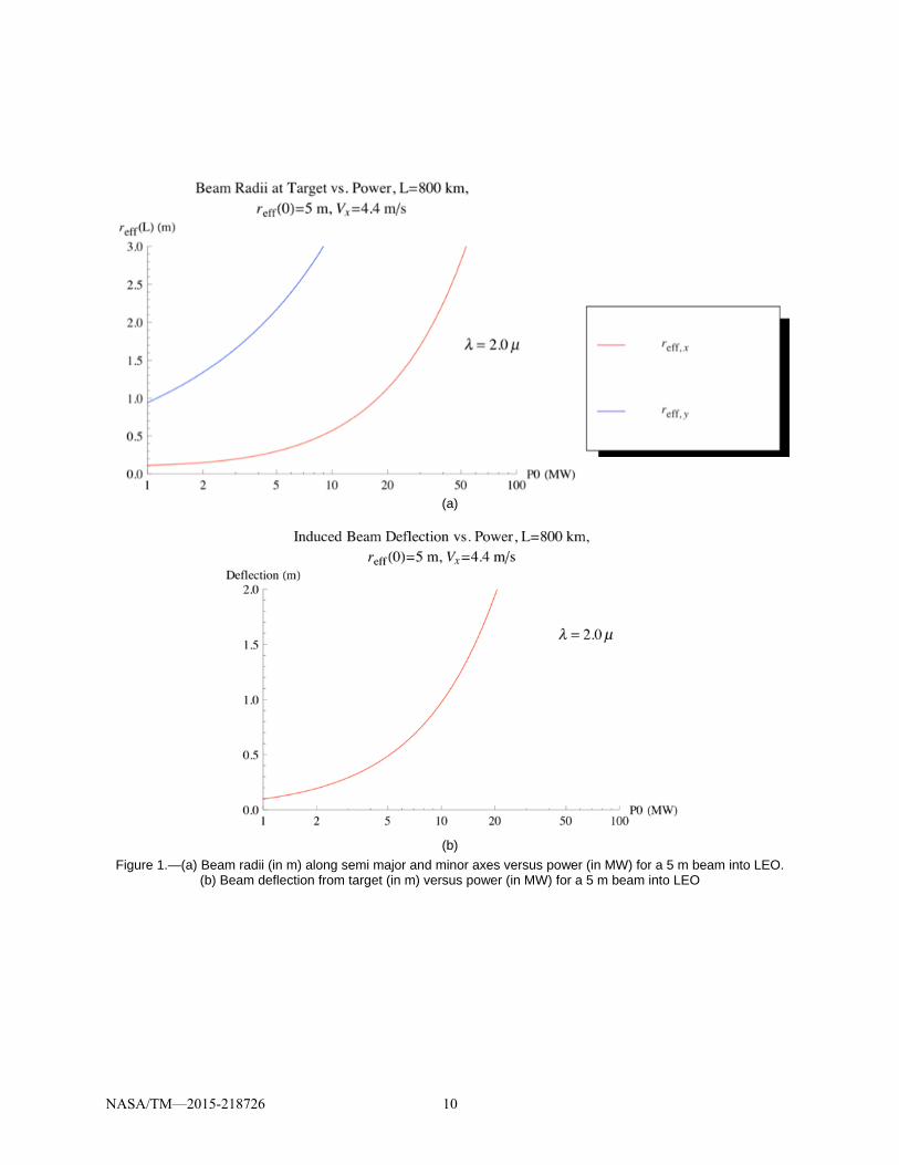
(a)

(b)

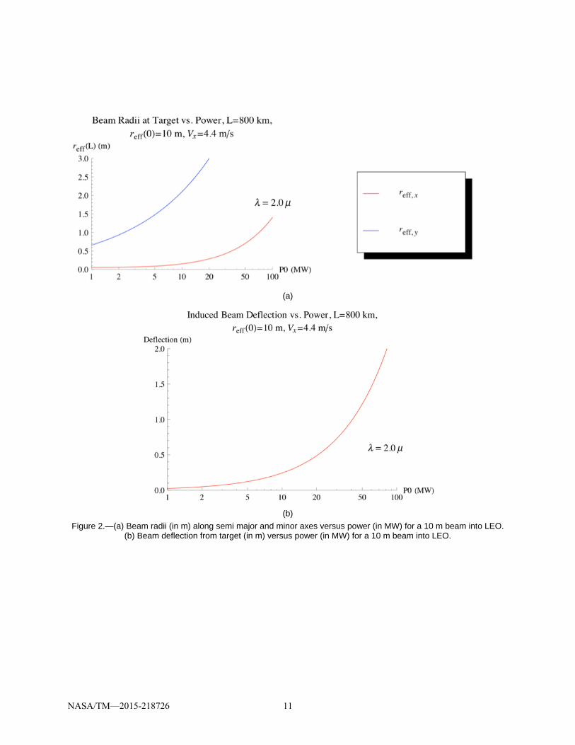
Figure 1.—(a) Beam radii (in m) along semi major and minor axes versus power (in MW) for a 5 m beam into LEO. (b) Beam deflection from target (in m) versus power (in MW) for a 5 m beam into LEO

NASA/TM—2015-218726 10

(a)

(b)

Figure 2.—(a) Beam radii (in m) along semi major and minor axes versus power (in MW) for a 10 m beam into LEO. (b) Beam deflection from target (in m) versus power (in MW) for a 10 m beam into LEO.

NASA/TM—2015-218726 11

(a)

(b)

Figure 3.—(a) Beam radii (in m) along semi major and minor axes versus power (in MW) for a 10 m beam into GEO. (b) Beam deflection from target (in m) versus power (in MW) for a 10 m beam into GEO.

NASA/TM—2015-218726 12

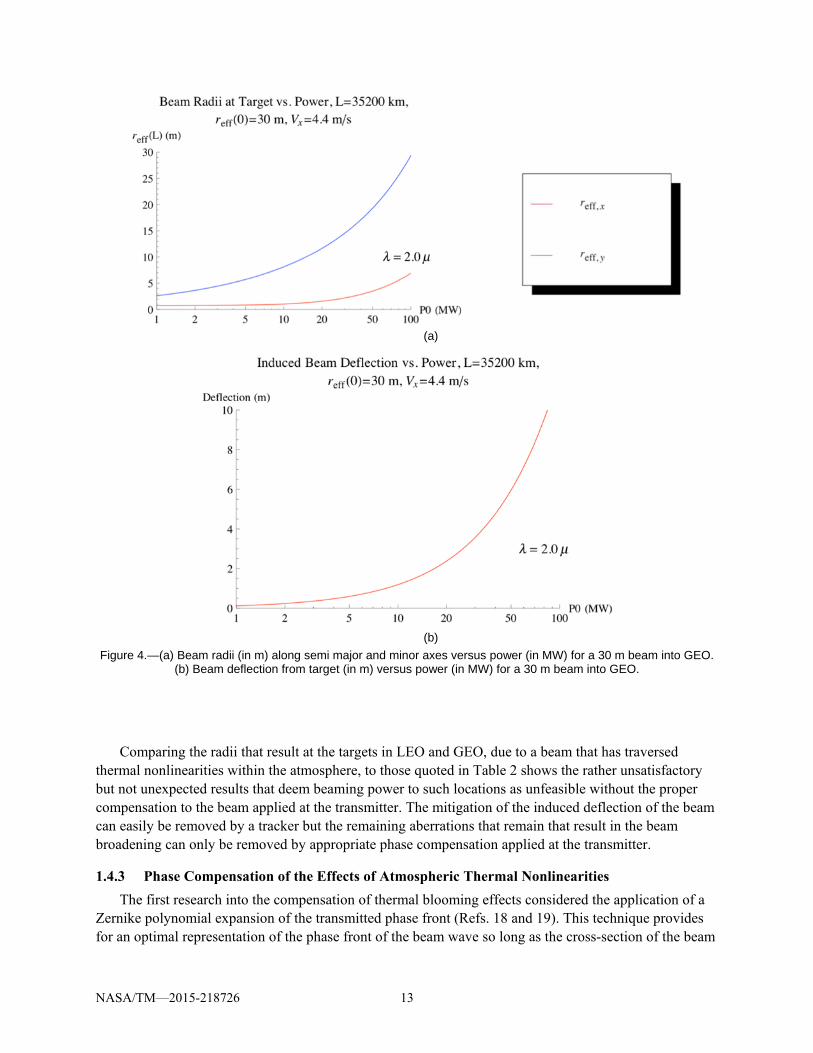
(a)

(b)

Figure 4.—(a) Beam radii (in m) along semi major and minor axes versus power (in MW) for a 30 m beam into GEO. (b) Beam deflection from target (in m) versus power (in MW) for a 30 m beam into GEO.

Comparing the radii that result at the targets in LEO and GEO, due to a beam that has traversed thermal nonlinearities within the atmosphere, to those quoted in Table 2 shows the rather unsatisfactory but not unexpected results that deem beaming power to such locations as unfeasible without the proper compensation to the beam applied at the transmitter. The mitigation of the induced deflection of the beam can easily be removed by a tracker but the remaining aberrations that remain that result in the beam broadening can only be removed by appropriate phase compensation applied at the transmitter.

1.4.3 Phase Compensation of the Effects of Atmospheric Thermal Nonlinearities The first research into the compensation of thermal blooming effects considered the application of a

Zernike polynomial expansion of the transmitted phase front (Refs. 18 and 19). This technique provides for an optimal representation of the phase front of the beam wave so long as the cross-section of the beam

NASA/TM—2015-218726 13

remains circular; after all, Zernike polynomials are, by design, orthogonal on a unit circle. The problem encountered in the above development is different; a beam asymmetry arises due to the differences in convective versus diffusion cooling of the atmospheric channel in which the beam propagates. The model briefly reviewed in Section 1.4.1 allows for the analytical assessment of phase compensation of the deleterious effects shown in Section 1.4.2.

The different behavior of the beam along the transverse axes suggest the use of a more general set of orthogonal polynomials than those of Zernike. Here, since the initial form of the beam wave is given by a Gaussian function, the transmitted phase front S(x,y) at the output aperture of the transmitter can be expanded in a set of orthogonal polynomials associated with a Gaussian weight function, i.e., the Hermite polynomials Hn(x) and Hm(y) (Ref. 20). Thus,

( ) ( ) ( ),M N

nm n mn m

S x y a H x H y=∑∑ (10)

The expansion coefficients anm are determined by applying one of several ‘performance metrics’. For example, for power beaming applications considered in this study, it is desired to shape the phase front so as to minimize the radius of the beam at the target so as not to have the beam interfere with the adjacent structures of the vehicle. Hence, the performance metric to be minimized through the selection of the anm is related to the electric field E″(ρ′,L) of the beam at the target vehicle by

( )( )

( )( )

2 3

0 2 2

2

0

,

,

,

E L d

L x y

E L d

∞

∞

′′ ′ ′ ′ρ ρ ρ

′ ′ ′Π ≡ ρ = +

′′ ′ ′ ′ρ ρ ρ

∫

∫ (11)

in which E″(ρ′,L) results from the application of the boundary condition

( ) ( )2

0,0 exp , , 12

dLE A iS x y iL

′ ρ′′ ′ ′ ′ ′ ′ ′ρ = − γ − γ ≡ +

(12)

to the solution of Equation (3). Ideally, the number of terms of the expansion given in Equation (10) is infinite, i.e., N,M → ∞. The linear terms for which n + m = 1 determine the inclination correction of the beam wave; the quadratic terms for which n + m = 2 determine the focusing correction and the higher order terms for which n + m ≥ 3 give the higher order aberration corrections. However, in realistic applications, the number of aberrations N and M is finite and, in fact, it is desired to find the smallest number of aberration corrections that can be used to represent the compensated phase. The specific expressions for the coefficients anm are found by equating to zero the derivative of Π(L) with respect to these coefficients.

The propagation problem defined here, as well as the associated minimization problem, can be solved analytically and will also appear in a forthcoming NASA Technical Memorandum. The results applied to the calculation of the phase-corrected beam radii are as follows. Due to the elliptical shape of the beam which is characterized by two radii at the target vehicle, it facilitates the calculations to consider a single effective radius ( )effr L′ defined by

NASA/TM—2015-218726 14

( )( ) ( )2 2

, ,

2eff x eff y

effr L r L

r L+

′ ≡ (13)

Applying the modeling procedure as outlined above, one finds for the radius ( ),eff Corrr L′ of a focused beam wave corrected for the first M phase aberrations represented by the model of Equation (10)

( ) ( ) ( ) ( ) ( ) ( ) ( )

( )

212 2

, 0 0 3( )/21 0

2

3 /20

0 01 2.95 4 2 ! !

2 ! !

02 !

4 2 !

M Mn m n meff Corr eff NLV NLV n m

n m

Mn nn

n

H Hr L R L P P n m n m

n m

Hn n

n

− ++

= =

=

′ = + Θ − Θ + π +

∑∑

∑

(14)

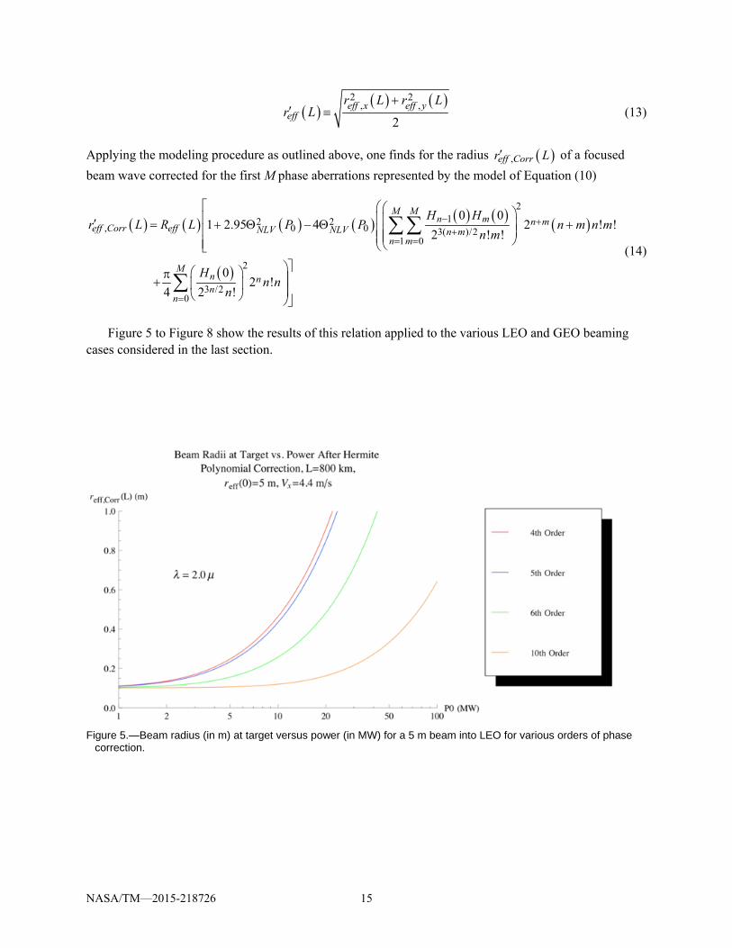
Figure 5 to Figure 8 show the results of this relation applied to the various LEO and GEO beaming cases considered in the last section.

Figure 5.—Beam radius (in m) at target versus power (in MW) for a 5 m beam into LEO for various orders of phase

correction.

NASA/TM—2015-218726 15

Figure 6.—Beam radius (in m) at target versus power (in MW) for a 10 m beam into LEO for various orders of phase

correction.

Figure 7.—Beam radius (in m) at target versus power (in MW) for a 10 m beam into GEO for various orders of phase

correction.

NASA/TM—2015-218726 16

Figure 8.—Beam radius (in m) at target versus power (in MW) for a 30 m beam into GEO for various orders of phase

correction.

These plots display the fact that for initial beam powers of 10 MW or less, phase correction using M = 10 order aberrations returns the radius of the beam to its desired value at the target vehicle. Beyond this power level, only the case shown in Figure 8 using a beam radius of 30 m at the transmitter can a 10th order phase correction be effective up to about 70 MW.

One assumption that has been prevailing in all these calculations is that the wind velocity V is a constant along the entire propagation path. In reality, this is certainly not the case and, in fact, there may be regions in which the V ≈ 0, i.e., a stagnation zone, and the convective heating scenario assumed here will transform into a diffusive heating one characterized by much lower critical power thresholds. This case will not be studied here, as it is the subject of a recent study (Ref. 21), but it must be kept in mind that a statistical description of the wind profile along the propagation path will be required in a more careful examination.

Finally, there is the whole issue of the effect that the beam profile will have on the level of thermal nonlinearity perturbations. In fact, very high-energy laser beams are characterized by initial beam profiles that are ‘tubular’, i.e., have a local minimum of intensity in the center which increases toward the outer portions of the beam. Such beams, which can be modeled by hyper Gaussian profiles, tend to be characterized by higher critical power thresholds. This is due to the fact that the center of the beam, with a lower intensity, is thermally cooler than the periphery and thus tends to bend toward the center and remain stable. This effect should be studied for the particular high-energy sources that will be used as the design of the power-beaming scenarios evolve.

NASA/TM—2015-218726 17

1.4.4 Using the Propagation Model for the Analysis of Millimeter Wave Beaming Within the Earth’s Atmosphere

The methodology developed above for the infrared power beaming case for LEO/GEO orbital transfer can be applied to the millimeter wave case for power beaming to vehicles launched from within the Earth’s atmosphere. The wavelength of concern here is λ = 2.0×10–3 m = 2.0 mm with an output aperture radius reff = 50 m. This gives Ld = 7.9×106 m. The propagation distances involved range from L = 20 km to L = 120 km. Although the beam will not be directly focused on the target vehicle (the dimensions being envisioned will require the beam to have a focal length just beyond the vehicle), for the purposes of this discussion, F ≈ L. The effective distance within the atmosphere responsible for most of the absorption at these wavelengths is H ≈ 1.8 km. Hence, the condition Ld /F H/Ld is easily met. Additionally, there is a characteristic length LT that is a measure of the distance at which thermally induced diffraction effects will occur. This characteristic length can be defined using the length Ld as well as the nonlinear distortion parameter RV given by Equation (A24). In fact, a detailed analysis similar to that given in Appendix A gives for the thermal diffraction distance

3

0

peffT

T

r C VL

P

π ρ=

ε α (15)

At the wavelength considered in this section, the associated absorption coefficient is α ≈ 2.2×10–4 m–1 which gives for the total transmitter power of P0 = 800 MW (which will be considered below), LT ≈ 73 km. Hence, thermal diffraction effects will certainly not prevail within the region H ≈ 1.8 km or, for that matter, within the entire troposphere and the model constructed above can be adopted here. (This circumstance is solely due to the very large output aperture that is being used.)

Equations (6) to (9) can now be used to consider four scenarios for a typical power-beaming launch:

1) Horizontal beaming (θ = 0°) at L = 20 km 2) Beaming at θ = 30°, L = 50 km 3) Beaming at θ = 50°, L = 100 km 4) Beaming at θ = 90°, L = 120 km

In each case, the target is to be illuminated in an area with a radius of Reff(L) ≈ 1.8 m. Thus, a dynamic focus is to be employed; the focal length is determined by

( )2

2, 1 12

d eff

d

kL R LL LFL L

= Φ = ± −Φ

(16)

where the ‘-‘ sign is used in front of the radical for a beam focused behind the target. The results of applying the propagation model to these cases are displayed in Figure 9 to Figure 12.

NASA/TM—2015-218726 18

(a)

(b)

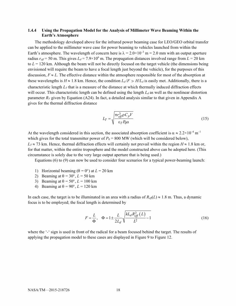
Figure 9.—(a) Beam radii (in m) along semi major and minor axes versus power (in MW) for a 50 m beam. (b) Beam deflection from target (in m) versus power (in MW) for a 50 m beam.

NASA/TM—2015-218726 19

(a)

(b)

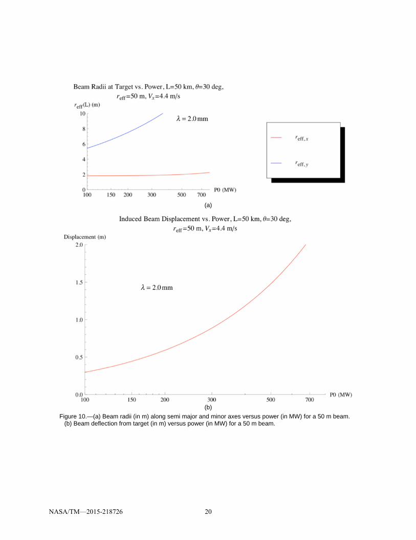
Figure 10.—(a) Beam radii (in m) along semi major and minor axes versus power (in MW) for a 50 m beam. (b) Beam deflection from target (in m) versus power (in MW) for a 50 m beam.

NASA/TM—2015-218726 20

(a)

(b)

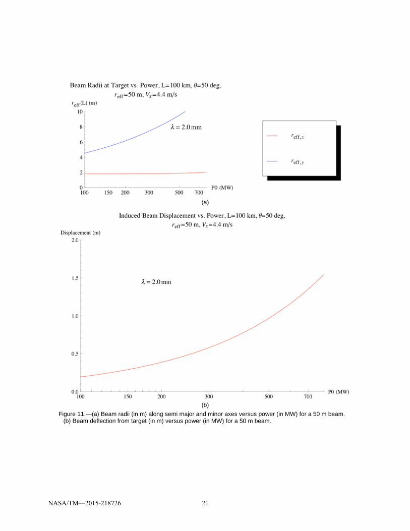
Figure 11.—(a) Beam radii (in m) along semi major and minor axes versus power (in MW) for a 50 m beam. (b) Beam deflection from target (in m) versus power (in MW) for a 50 m beam.

NASA/TM—2015-218726 21

(a)

(b)

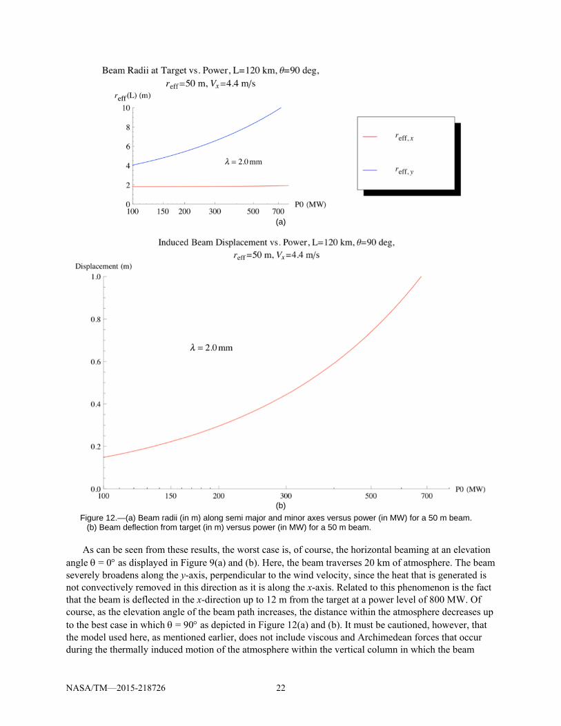
Figure 12.—(a) Beam radii (in m) along semi major and minor axes versus power (in MW) for a 50 m beam. (b) Beam deflection from target (in m) versus power (in MW) for a 50 m beam.

As can be seen from these results, the worst case is, of course, the horizontal beaming at an elevation

angle θ = 0° as displayed in Figure 9(a) and (b). Here, the beam traverses 20 km of atmosphere. The beam severely broadens along the y-axis, perpendicular to the wind velocity, since the heat that is generated is not convectively removed in this direction as it is along the x-axis. Related to this phenomenon is the fact that the beam is deflected in the x-direction up to 12 m from the target at a power level of 800 MW. Of course, as the elevation angle of the beam path increases, the distance within the atmosphere decreases up to the best case in which θ = 90° as depicted in Figure 12(a) and (b). It must be cautioned, however, that the model used here, as mentioned earlier, does not include viscous and Archimedean forces that occur during the thermally induced motion of the atmosphere within the vertical column in which the beam

NASA/TM—2015-218726 22

propagates. For situations in which large elevation angles are realized, these effects must be included in a future extension of the analysis. Finally, it must be noted that in order to follow the relatively close target vehicle, the beam will have a discernable slewing velocity as compared to that of the LEO/GEO transfer case discussed earlier. This slewing velocity may (depending on the relative wind velocity) tend to lessen the thermal effects. This will certainly be the case for the upward movement of the beam. As for the horizontal component of the slewing velocity, it can either detract or worsen the thermal effects. Such aspects of the problem can only be assessed via a simulation of the particular launch environment.

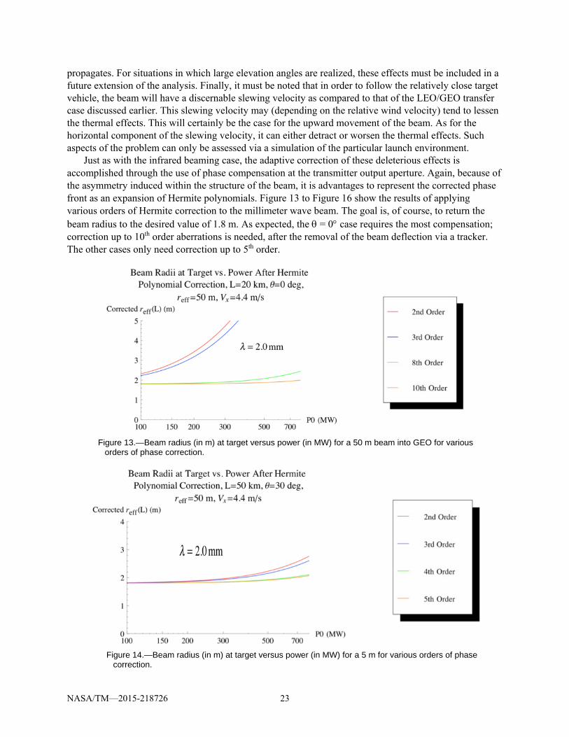
Just as with the infrared beaming case, the adaptive correction of these deleterious effects is accomplished through the use of phase compensation at the transmitter output aperture. Again, because of the asymmetry induced within the structure of the beam, it is advantages to represent the corrected phase front as an expansion of Hermite polynomials. Figure 13 to Figure 16 show the results of applying various orders of Hermite correction to the millimeter wave beam. The goal is, of course, to return the beam radius to the desired value of 1.8 m. As expected, the θ = 0° case requires the most compensation; correction up to 10th order aberrations is needed, after the removal of the beam deflection via a tracker. The other cases only need correction up to 5th order.

Figure 13.—Beam radius (in m) at target versus power (in MW) for a 50 m beam into GEO for various

orders of phase correction.

Figure 14.—Beam radius (in m) at target versus power (in MW) for a 5 m for various orders of phase

correction.

NASA/TM—2015-218726 23

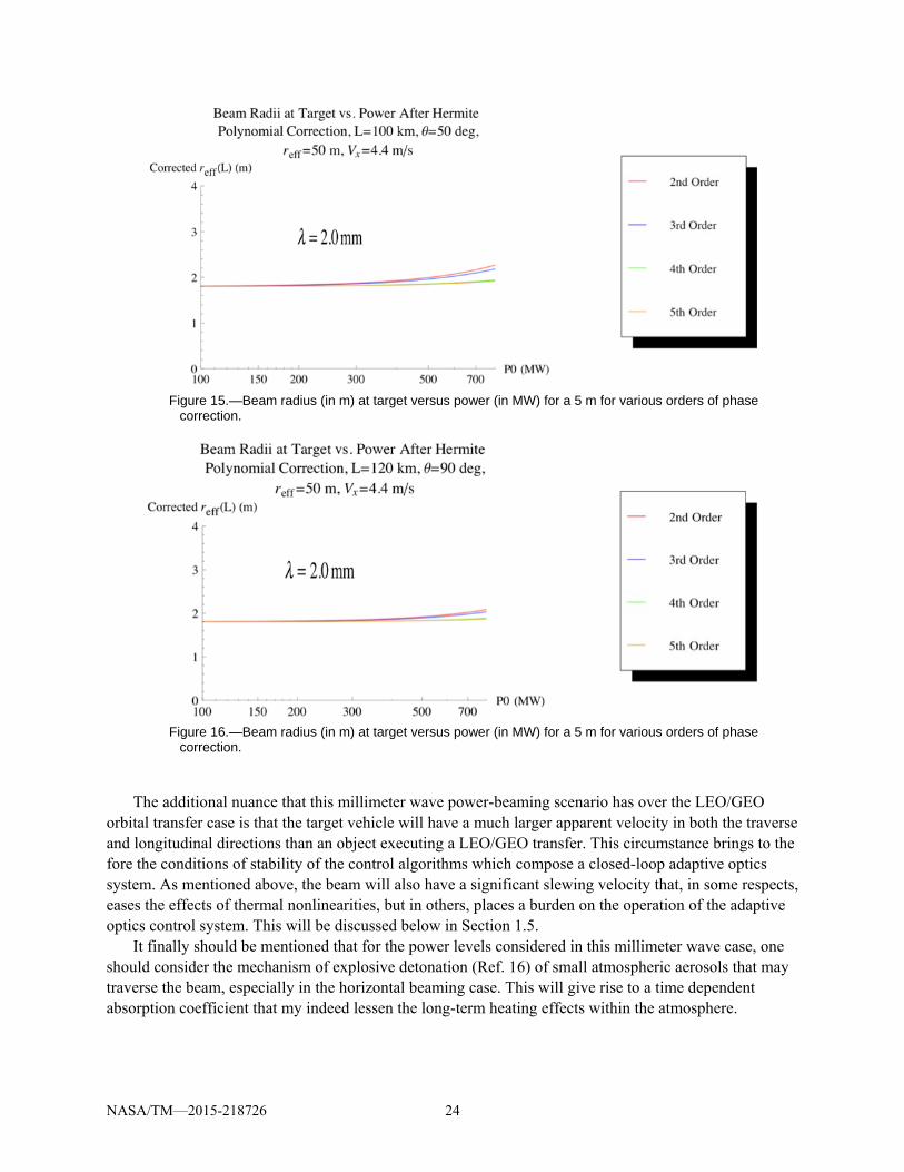
Figure 15.—Beam radius (in m) at target versus power (in MW) for a 5 m for various orders of phase

correction.

Figure 16.—Beam radius (in m) at target versus power (in MW) for a 5 m for various orders of phase

correction.

The additional nuance that this millimeter wave power-beaming scenario has over the LEO/GEO orbital transfer case is that the target vehicle will have a much larger apparent velocity in both the traverse and longitudinal directions than an object executing a LEO/GEO transfer. This circumstance brings to the fore the conditions of stability of the control algorithms which compose a closed-loop adaptive optics system. As mentioned above, the beam will also have a significant slewing velocity that, in some respects, eases the effects of thermal nonlinearities, but in others, places a burden on the operation of the adaptive optics control system. This will be discussed below in Section 1.5.

It finally should be mentioned that for the power levels considered in this millimeter wave case, one should consider the mechanism of explosive detonation (Ref. 16) of small atmospheric aerosols that may traverse the beam, especially in the horizontal beaming case. This will give rise to a time dependent absorption coefficient that my indeed lessen the long-term heating effects within the atmosphere.

NASA/TM—2015-218726 24

1.4.5 A Tool for the Quick Assessment of Nonlinear Thermal Effects on Power Beaming Appendix A introduced several expressions for threshold power levels at which thermal effects will

become prevalent. Although these derivations were essentially based on normalization and dimensional analysis, they can be given credence by using the results obtained above. However, these critical power levels need to be related to a specific property or characteristic of a beam wave that will impact the performance of the power beaming system. As there are many such characteristics, there too will be as many corresponding critical power levels; there is no single universal quantity that can be stated to convey the specific impact thermal blooming will have on the entire performance of a beamed energy system. However, the most important characteristic in power-beaming situations is the variation of the beam radius due to the defocusing that occurs during the heating of the atmosphere. As shown by Equation (7) and, e.g., in Figure 1 to Figure 4, the radius of a beam in an atmosphere with convection is severely perturbed in the direction perpendicular to the wind direction. In order to attempt to secure an analytical estimate at which the radius of such a beam will begin to increase due to thermal blooming, one can expand Equation (7) and get

( ) ( ) ( ), 00.8661

2d

eff y eff NLVLr L R L PL

= + Θ +

(17)

and require the value for P0 at which

( ) ( )2 00

00.866 0.1 12

eff TdNLV

p

k r P HL PL C VL

ε αΘ ≈ =

πρ (18)

Setting L = H, one finally obtains for the critical power PcrR at which the beam radius begins to expand

( )2100p

crReff T

C VP

k rπρ

=ε α

(19)

which is just 10PcrT as obtained in the Appendix A. One can now use this relation for millimeter wavelengths and compare to the infrared case. Figure 17 and Figure 18 show plots of Equation (19), as well as the associated power density ( )2 0crR effP rπ , versus aperture radius for both cases. Here, the

nominal wind velocity is taken to be V = 0.5 m/s. Of course, Equation (19) is simple enough to apply a statistical model describing the value for V.

Evaluating Equation (19) using the numerical values of the parameters that do not depend on the wavelength, one has for this critical power

2

200 MWcrReff

Prλ

=α

(20)

where PcrR is in MW and λ and reff are in meters. (The units of α are m–1.) These results clearly show that propagation at millimeter wavelengths within the atmosphere can sustain much larger power levels than at infrared wavelengths.

NASA/TM—2015-218726 25

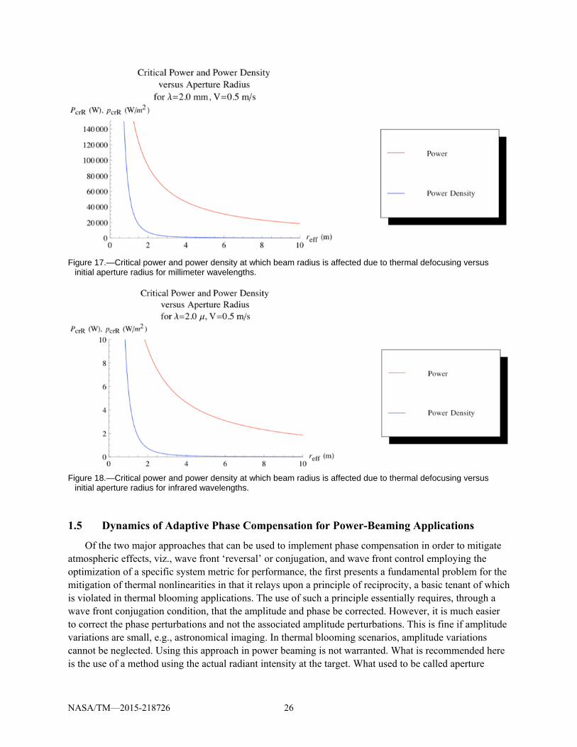
Figure 17.—Critical power and power density at which beam radius is affected due to thermal defocusing versus

initial aperture radius for millimeter wavelengths.

Figure 18.—Critical power and power density at which beam radius is affected due to thermal defocusing versus

initial aperture radius for infrared wavelengths.

1.5 Dynamics of Adaptive Phase Compensation for Power-Beaming Applications

Of the two major approaches that can be used to implement phase compensation in order to mitigate atmospheric effects, viz., wave front ‘reversal’ or conjugation, and wave front control employing the optimization of a specific system metric for performance, the first presents a fundamental problem for the mitigation of thermal nonlinearities in that it relays upon a principle of reciprocity, a basic tenant of which is violated in thermal blooming applications. The use of such a principle essentially requires, through a wave front conjugation condition, that the amplitude and phase be corrected. However, it is much easier to correct the phase perturbations and not the associated amplitude perturbations. This is fine if amplitude variations are small, e.g., astronomical imaging. In thermal blooming scenarios, amplitude variations cannot be neglected. Using this approach in power beaming is not warranted. What is recommended here is the use of a method using the actual radiant intensity at the target. What used to be called aperture

NASA/TM—2015-218726 26

optimization or ‘tagging’ (Ref. 22), has now come to be known as target-in-the-loop and its implementation is known as ‘gradient descent optimization (GDO) wave front control’ (Refs. 23 to 27) and is suggested for the power beaming applications addressed in this report. Here, the control rule is based on the direct optimization of an easily measured system performance metric, such as the radiant intensity at the target.

The model governing the operation of such an adaptive optics system is given by first identifying a performance metric ( )S aΠ ≡Π

as defined by Equation (11) that is dependent upon the phase given by

Equation (10) and the array [ ]nma a= of associated expansion coefficients (Ref. 24). The coefficients in

Equation (10) were selected for modeling purposes based on the minimization of the beam radius on the target vehicle. Here, the optimal selection of the values of anm during the actual operation of the system is given by the control rule

( ) ( )

nmnm

anm

a t tt a

∂ ∂Πτ = −γ

∂ ∂ (21)

in which τnm are the time constants and γ is the control (or ‘update’) coefficient. Here, J will be taken to be the size of the focal spot at the target vehicle. The intensity can be inferred by recording the reflected radiation form the target at a point separated from the transmitter so that a slightly different and unperturbed propagation path is used. It must now be established that such a control structure will dynamically operate in the two extreme cases of power beaming considered here, i.e., infrared beaming to a vehicle in GEO and millimeter wave beaming to a near Earth vehicle.

Consider first power-beaming to GEO. For purposes of a brief analysis in which the required temporal characteristics of the adaptive optics system (and thus the temporal stability) are to be derived, one can consider the isolated case for which n + m = 2, i.e., according to the discussion in Section 1.4.3, the dynamic focusing of the beam wave. Thus, one has from Equation (10) for the associated (now time dependent) aberration coefficient

( )20 ( )dLa t

F t= (22)

where, e.g., H2(x) ~ x2. For the case in which the focus is to be placed at the target at a distance L, i.e., F(t) = L, and the one has from Equation (21),

( ) ( )20 20 0 expd d

a

L L ta t aL L t

= + + − (23)

where ( )2 220a dt L L= τ γ is the adaptation time of the adaptive optics system. This very important time

constant is, although proportional to τ20, inversely proportional to the distance to the target. This well-known property has it that the adaptive system will possess a faster response the farther the target from the transmitter. If this were all that the description of the adaptation system required, then the state of focusing on the target will monotonically approach the desired result Ld/L. However, there is a limiting factor placed on this circumstance by the delay inherent in overall system response do to the propagation time to and from GEO. When the propagation delay is allowed to enter into the control rule, Equation (21) now becomes

NASA/TM—2015-218726 27

( ) ( )

nmnm d

anm

a t t tt a

∂ ∂Π −τ = −γ

∂ ∂ (24)

where td is the delay time (in this case, light time to and from the target). Expanding the right side of this equation in a Taylor series in td and keeping the first few terms yields

( ) ( ) ( ) ( )22 2

22nmnm d

a dnm nm d nm d

ta t t t tt

t a a t a t ∂ ∂Π ∂ Π ∂ Π

τ = −γ − + − ∂ ∂ ∂ ∂ ∂ ∂

(25)

The corresponding characteristic equation ς for the resulting differential relationship for a20 (t) = exp(–ςt) in the example considered above is given by

22

2

2a d a a d d

d

t t t t t tt±

− ± − −ς = (26)

shows that the system converges to a stable state so long as ta > td, i.e., the adaptation period of the system is longer than the delay time. For a target in LEO, td ≥ 0.005 sec and for GEO, td ≈ 0.24 sec (for the round trip time). If, on the other hand td > ta, the system does not converge to the stable state and

( )20limt

a t→∞

→∞ . Thus, the adaptive system must be continuously ‘tuned’ (by adjusting γ in response to

changes in td as well as the evolving values for L in the case of a moving target) so that the condition ta > td is satisfied.

To these considerations must also be added the temporal delay in the overall system response. This will not be discussed here as these considerations can be found in the literature. Suffice it to say that the delay that is met with in beaming to GEO can be easily factored into the operation of the adaptive system. It must be remembered that the distance to the target is always increasing in time for a beamed power scenario and this, above and beyond that of the propagation delay, must be properly treated in the design and specification of the adaptive optics control system.

Work on the actual implementation of the close-loop control of the gradient descent algorithm of Equation (21) has rapidly progressed. The technology is now mature and forms the basis for reliable adaptive control. The only possible nuance to its application is for power beaming to locations within the Earth’s atmosphere for surface or near-surface launching. Here, the target vehicle, unlike the LEO/GEO transfer case, is rapidly moving and is considered an extended target, i.e., its spatial extent cannot be relegated to a point object and its possible rotation and orientation becomes an issue for use as a reflector of radiation bask to the adaptive optics receiver. Here, the randomly rough surface of the target reflector creates a speckle field characterized by bright and dark regions of intensity has been found to complicate the implementation of a closed loop adaptive optics scenario. This can lead to the slowing of the convergence speed of the system and, ultimately, to the efficiency of its operation in terms of the optimization of the focal spot at the target. Methods using the pre-compensation of the beam show promise (Ref. 28).

Although it has been shown above that the basic physics of the situation does not preclude beaming energy to a prescribed area on a target vehicle in GEO, the engineering implementation will offer some major obstacles to be negotiated. In particular, the beaming into a GEO location will require 30 nanoradian pointing accuracy on the part of the transmitter optics. The presence of mechanical jitter of the transmitter platform must be continuously mitigated. Additionally, on the other side of the spectrum,

NASA/TM—2015-218726 28

launching from within the atmosphere will challenge the application of the adaptive optics at millimeter wavelengths. The fact that the beam is rapidly slewing due to the relatively rapidly moving object makes it difficult for the closed-loop adaptive optics system to converge to a stationary value since the medium within the column of atmosphere in which the millimeter wave beam exists is constantly being exchanged. Here, instead of employing the target as the beacon source, the use of an artificial beacon placed ahead of the moving vehicle may help in characterizing the atmosphere ahead of the beam. This will assess the phase perturbations of the nonheated atmosphere but the problem still remains concerning just how the atmosphere will respond to the heating from the beam as it arrives at that particular column. This suggests that, due to the availability of high power sources at millimeter wavelengths, one configure an in situ experiment to assess the operation of both closed-loop versus artificial beacon adaptive optics approaches. This will be discussed further below.

1.6 Experiments Assessing the Compensation of Thermal Nonlinearities of High Power Beams in the Atmosphere

Experiments dealing with the induced effects due to thermal nonlinearities elicited by high power propagation are usually performed in a laboratory using liquids placed in cells in which the thermal nonlinearity thresholds are much smaller than in air. In these scaled laboratory experiments, where atmospheric turbulence effects are simulated by transmission phase screens, various adaptive optics algorithms have been tested and evaluated (Refs. 29 and 30). Some experiments have been performed in the open atmosphere along horizontal paths in a program called the Scaled Atmospheric Blooming Experiments (SABLE) directed by Lincoln Laboratory (Ref. 31). Work is also continuing along these lines in other countries (Refs. 32). All these experiments endeavor to evaluate the in situ operation of adaptive optics systems on a scaled basis. The same must be recommended for the operation of a beamed power scenarios discussed above. Due to the maturity and availability of high power sources in the millimeter range, it is recommenced that a scaled atmospheric experiment be performed on a moving target to assess the operation of various adaptive optics algorithms. Such an experiment should be modeled after the SABLE project. It is important to note that there currently does not exist a database that addresses the power beaming cases considered here. It is important to begin to capture the prevailing effects and system operation using a scaled atmospheric experiment which would simulate the realistic environment in which an adaptive optics system must operate, from the variable wind velocity up to the mechanical jitter of the transmitter platform. Additionally, this experimental scenario can also be used to address the issue related to the possibility of air ionization, and subsequent breakdown, across the apertures of the combined millimeter wave gyrotron sources as discussed elsewhere in this report.

1.7 Conclusions and Recommendations

The various deleterious propagation mechanisms associated with high-power electromagnetic wave propagation through the atmosphere have been discussed. In addition to turbulence, thermal nonlinearities associated with the absorption of radiation by the atmospheric gas will contribute to the major effects of beam wave propagation for beamed energy propulsion at the power levels considered here. The simplified propagation model advanced here shows that the beam radius as well as its deflection are severely affected by the phenomena of thermal blooming. However, the model also showed that appropriate phase compensation at the transmitter output aperture can mitigate these effects and return the propagation situation to one that is acceptable for the power transfer requirements that are needed to be satisfied for beamed propulsion. For infrared transmission out of the atmosphere for LEO/GEO beaming, up to 10th order (once the tilt has been removed) aberration correction will be needed in order to maintain a minimal

NASA/TM—2015-218726 29

focal spot at a GEO location using a 30 m diameter transmitter aperture. For millimeter wave beaming within the atmosphere, 5th order aberration correction will suffice with the exception of the horizontal case in which, once again, a 10th order correction would be requires. In principle, these corrections allow the beaming system to operate within the prevailing specifications. In practice, however, some challenges prevail in the implementation.

The adaptive optics approach recommended here for the LEO/GEO launch case is a closed-loop system that uses the specular reflection from the target vehicle as a ‘beacon’ source (i.e., a target-in-the-loop system). The target vehicle is seen by the adaptive optics system as a simple point reflector. The round-trip propagation time delay inherent in this scenario can be tolerated so long as the adaptation time of the adaptive optics system is properly set to a slightly larger time than that of the delay to assure proper convergence.

In the case of millimeter wave beaming to a moving vehicle within the Earth’s atmosphere, the object is now considered as an extended target the rotation and orientation of which can complicate application of the closed loop system. The reflection from the vehicle will posses a speckle structure that can severely impact the wave front sensor used by the adaptive optics system. Here, it may be that the simpler artificial beacon method can be used but there is still an additional complication, viz., the rapid movement of the beam across the atmosphere. The changes induced in the beam column through the atmosphere will not all be those due to the adjustment by the adaptive optics and the system will not be able to properly adapt. This situation presents itself for a scaled atmospheric high-power millimeter wave transmission experiment in which both closed loop and artificial beacon-based adaptive optics systems are tested and evaluated.

The propagation modeling for the various beamed propulsion scenarios presented in this report should be extended beyond that employed here in Section 1.4 by incorporating additional fluid mechanical descriptions of the atmosphere as well as more general beam wave profiles such as hypergaussian as well as fractional charge (in the topological sense) Laguerre-Gaussian beam waves which show great promise in their ability to be robust with respect to atmospheric nonlinearities (Ref. 33). However, it is important that the modeling effort be kept to the level of yielding analytical results, rather than requiring numerical evaluation, so as to capture all the nuances of the physics involved and, at the same time, provide a tool for overall system evaluation as well as the design of adaptive optics algorithms. Finally, the model should be incorporated into a trajectory analysis program so a cadre of launch geometries can be evaluated from the point of view of atmospheric thermal nonlinearities.

NASA/TM—2015-218726 30

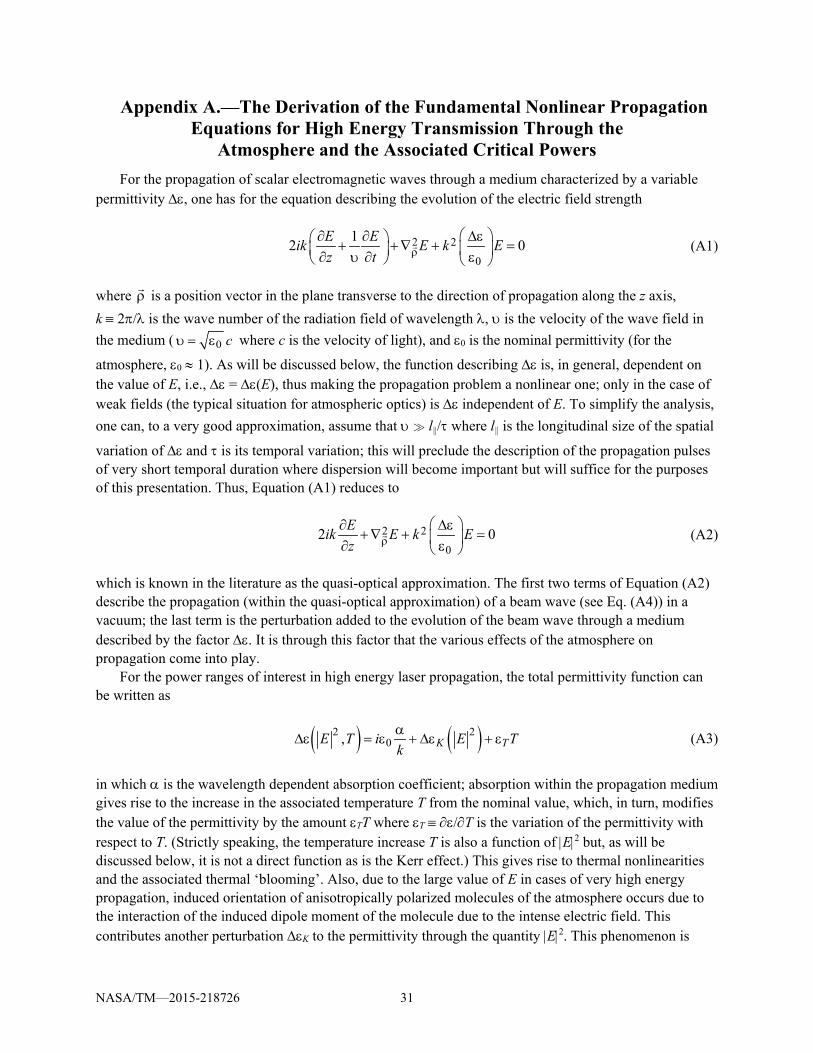
Appendix A.—The Derivation of the Fundamental Nonlinear Propagation Equations for High Energy Transmission Through the

Atmosphere and the Associated Critical Powers For the propagation of scalar electromagnetic waves through a medium characterized by a variable

permittivity ∆ε, one has for the equation describing the evolution of the electric field strength

2 2

0

12 0E Eik E k Ez t ρ

∂ ∂ ∆ε + +∇ + = ∂ υ ∂ ε (A1)

where ρ

is a position vector in the plane transverse to the direction of propagation along the z axis, k ≡ 2π/λ is the wave number of the radiation field of wavelength λ, υ is the velocity of the wave field in the medium ( 0 cυ = ε where c is the velocity of light), and ε0 is the nominal permittivity (for the

atmosphere, ε0 ≈ 1). As will be discussed below, the function describing ∆ε is, in general, dependent on the value of E, i.e., ∆ε = ∆ε(E), thus making the propagation problem a nonlinear one; only in the case of weak fields (the typical situation for atmospheric optics) is ∆ε independent of E. To simplify the analysis, one can, to a very good approximation, assume that υ l

/τ where l

is the longitudinal size of the spatial

variation of ∆ε and τ is its temporal variation; this will preclude the description of the propagation pulses of very short temporal duration where dispersion will become important but will suffice for the purposes of this presentation. Thus, Equation (A1) reduces to

2 2

02 0Eik E k E

z ρ ∂ ∆ε

+∇ + = ∂ ε (A2)

which is known in the literature as the quasi-optical approximation. The first two terms of Equation (A2) describe the propagation (within the quasi-optical approximation) of a beam wave (see Eq. (A4)) in a vacuum; the last term is the perturbation added to the evolution of the beam wave through a medium described by the factor ∆ε. It is through this factor that the various effects of the atmosphere on propagation come into play.

For the power ranges of interest in high energy laser propagation, the total permittivity function can be written as

( ) ( )2 20, K TE T i E T

kα

∆ε = ε + ∆ε + ε (A3)

in which α is the wavelength dependent absorption coefficient; absorption within the propagation medium gives rise to the increase in the associated temperature T from the nominal value, which, in turn, modifies the value of the permittivity by the amount εTT where εT ≡ ∂ε/∂T is the variation of the permittivity with respect to T. (Strictly speaking, the temperature increase T is also a function of |E|2 but, as will be discussed below, it is not a direct function as is the Kerr effect.) This gives rise to thermal nonlinearities and the associated thermal ‘blooming’. Also, due to the large value of E in cases of very high energy propagation, induced orientation of anisotropically polarized molecules of the atmosphere occurs due to the interaction of the induced dipole moment of the molecule due to the intense electric field. This contributes another perturbation ∆εK to the permittivity through the quantity |E|2. This phenomenon is

NASA/TM—2015-218726 31

known as the Kerr effect. The functional relations of both ( )2K E∆ε and T to the quantity |E|2 are also

given through the prescription of a differential equation. Each of these contributions will be separately discussed below and the critical field powers at which they will occur within the atmosphere will be derived. Before this is done, however, it will prove to be convenient to make the following digression concerning the description of a beam wave.

The consideration of the general solution for Equation (A2) makes it necessary to have an expression for the associated boundary condition. This brings to the fore the normalization of spatial coordinates. The boundary condition is given by the expression for the general form of a Gaussian beam wave, viz.,

( )20, exp

1 2 1A kE zi z i z

γ ρ ρ = − + γ + γ

(A4)

where A0 is the initial amplitude of the field and

1 2 1 220

2 1, ,ikW F

γ ≡ γ + γ γ ≡ γ ≡ (A5)

with W0 being the waist radius of the beam at the exit of the output aperture and F is the focal length. The initial condition for the field at the output aperture is thus given by

( )2

2 20 0 20

1 2,0 exp exp2 2k kE A A i

W F γ ρ ρ = − ρ = − ρ +

(A6)

At this point, it is convenient to normalize the spatial coordinates with respect to the parameters of the problem. For example, if one defines the ‘effective’ radius of the beam wave at the exit of the output aperture as 0 2effr W≡ , (this definition is consistent with the definition for the power distribution in

the transverse plane) one can define the dimensionless transverse coordinate ρ′ ≡ ρ/reff and write Equation (A6) as

( )2

02 201 1,0 exp2 2

kWE A i

F

′ ′ ′ρ = − ρ + ρ

(A7)

One can now apply the same coordinate normalization to Equation (A2). That is, since

( ) ( )2 22

0

2, ,E z E zW ′ρ ρ ′ ′∇ ρ = ∇ ρ

(A8)

Equation (A2) can be written (letting ε0 = 1 for atmospheric scenarios)

2 2 2

20 02 02 2

kW k WEi E Ez ′ρ

∆ε∂+∇ + =

∂ (A9)

NASA/TM—2015-218726 32

Now, normalizing the longitudinal coordinate z with respect to the quantity defined by 20 2dL kW≡ , i.e.,

z′ = z/Ld, and noting that

( ) ( )2

0

, ,2E z E zz kW z

′ ′∂ ρ ∂ ρ=

′∂ ∂

(A10)

Equations (A7) and (A9) become

( )2

0,0 exp 12

dLE A iF

′ ρ ′ρ = − +

(A11)

and

( )22 222 , 0effEi E k r E T Ez ′ρ∂

+∇ + ∆ε =′∂

(A12)

This form of the quasi-optical equation will facilitate the developments that follow. The quantity Ld is called the diffraction length and, as seen from Equation (A11), is the length that the focus must achieve for the associated diffraction to become appreciable.

A.1 The Critical Power for the Atmospheric the Kerr Effect To isolate the effect of the Kerr nonlinearity from the thermal effects due to absorption, one simply

lets ∆ε = ∆εK (|E|2) in Equation (A12) and obtains

( )22 222 0KeffEi E k r E Ez ′ρ∂

+∇ + ∆ε =′∂

(A13)

The differential equation that governs the evolution of ∆εK is given by

2KK K E

t∂∆ε

τ + ∆ε = ε∂

(A14)

where τ is the relaxation constant for the Kerr process and εK is the Kerr constant for the atmosphere; typically, τ ≈ 10–11 sec. Relative to the other processes to be considered (and the fact that very short pulse lengths are not being considered here), one can ignore the first term on the left of Equation (A14). In this case, ∆εK = εK|E|2 and Equation (A13) becomes

22 222 0KeffEi E k r E Ez ′ρ∂

+∇ + ε =′∂

(A15)

In the literature, Equation (A15) is sometimes stated to describe a ‘cubic’ medium due to the occurrence of E in the last term. Connecting |E|2 to the associated intensity I of the beam using the relation |E|2 = (8π/c)I and then to the corresponding beam power P0 using 2

0 effP r I= π , Equation (A15) becomes

NASA/TM—2015-218726 33

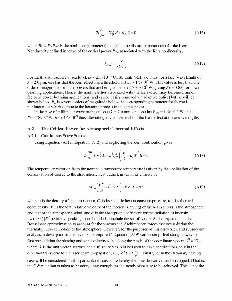
22 0KEi E R Ez ′ρ∂

+∇ + =′∂

(A16)

where RK ≡ P0/PcrK is the nonlinear parameter (also called the distortion parameter) for the Kerr Nonlinearity defined in terms of the critical power PcrK associated with the Kerr nonlinearity,

28crKK

cPk

=ε

(A17)

For Earth’s atmosphere at sea level, εK ≈ 2.5×10–16 CGSE units (Ref. 8). Thus, for a laser wavelength of λ = 2.0 µm, one has that the Kerr effect has a threshold at PcrK ≈ 1.5×109 W. This value is less than one order of magnitude from the powers that are being considered (~70×106 W, giving RK ≈ 0.05) for power beaming applications. Hence, the nonlinearities associated with the Kerr effect may become a minor factor in power beaming applications (and can be easily removed via adaptive optics) but, as will be shown below, RK is several orders of magnitude below the corresponding parameter for thermal nonlinearities which dominate the beaming process in the atmosphere.

In the case of millimeter wave propagation at λ = 2.0 mm, one obtains PcrK = 1.5×1016 W and at P0 = 70×106 W, RK ≈ 4.6×10–9 thus alleviating any concerns about the Kerr effect at these wavelengths.

A.2 The Critical Power for Atmospheric Thermal Effects A.2.1 Continuous Wave Source

Using Equation (A3) in Equation (A12) and neglecting the Kerr contribution gives

2 2 22 0eff TEi E k r i T Ez k′ρ∂ α +∇ + + ε = ′∂

(A18)

The temperature variation from the nominal atmospheric temperature is given by the application of the conservation of energy to the atmospheric heat budget, given in its entirety by

2pTC V T T It

∂ ρ + ⋅∇ = κ∇ + α ∂

(A19)

where ρ is the density of the atmosphere, Cp is its specific heat at constant pressure, κ is its thermal conductivity, V

is the total relative velocity of the motion (slewing) of the beam across is the atmosphere

and that of the atmospheric wind, and α is the absorption coefficient for the radiation of intensity I ≡ (c/8π) |E|2. (Strictly speaking, one should also include the set of Navier-Stokes equations in the Boussinesq approximation to account for the viscous and Archimedean forces that occur during the thermally induced motion of the atmosphere. However, for the purposes of this discussion and subsequent analysis, a description at this level is not required.) Equation (A19) can be simplified straight away by first specializing the slewing and wind velocity to be along the x axis of the coordinate system, ˆV Vx=

,

where x̂ is the unit vector. Further, the diffusivity ∇2T will be taken to have contributions only in the direction transverse to the laser beam propagation, i.e., 22T Tρ∇ ≈ ∇ . Finally, only the stationary heating

case will be considered for this particular discussion whereby the time derivative can be dropped. (That is, the CW radiation is taken to be acting long enough for the steady state case to be achieved. This is not the

NASA/TM—2015-218726 34

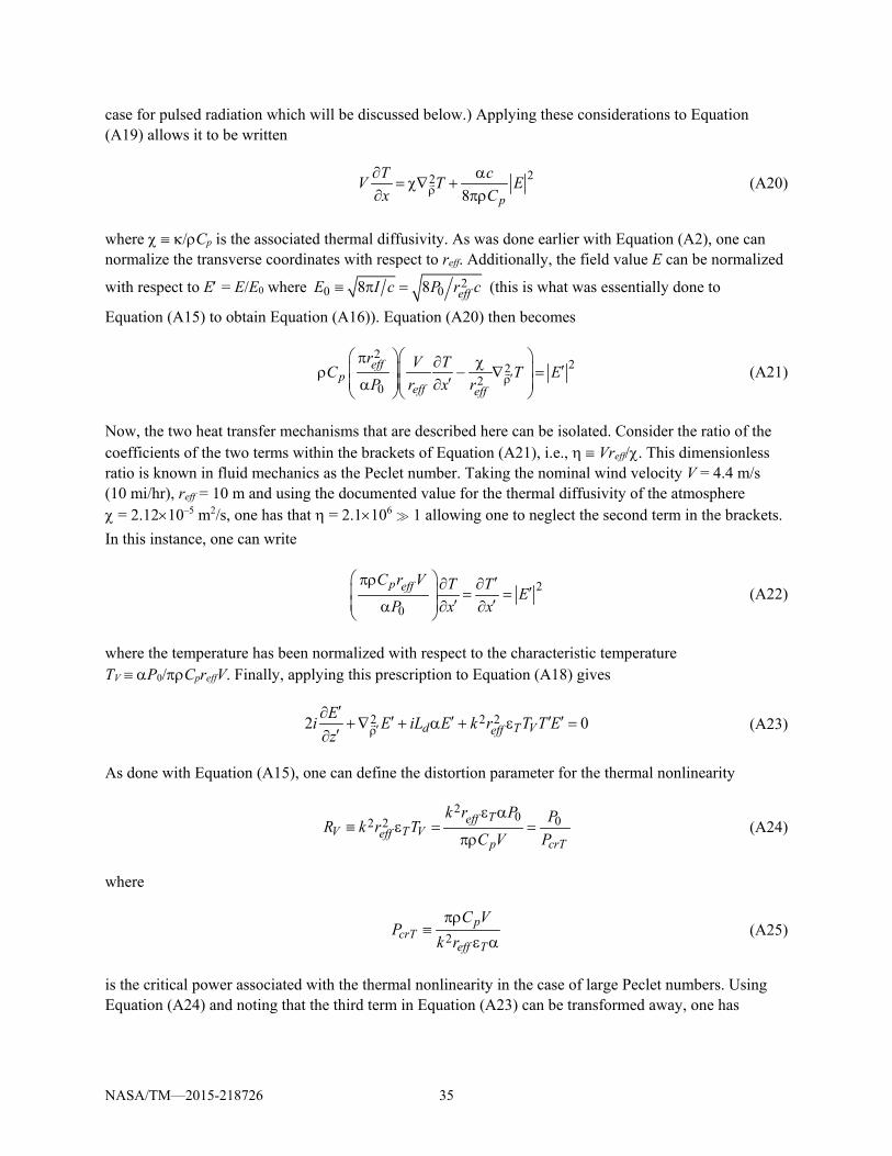
case for pulsed radiation which will be discussed below.) Applying these considerations to Equation (A19) allows it to be written

228 p

T cV T Ex Cρ

∂ α= χ∇ +

∂ πρ (A20)

where χ ≡ κ/ρCp is the associated thermal diffusivity. As was done earlier with Equation (A2), one can normalize the transverse coordinates with respect to reff. Additionally, the field value E can be normalized

with respect to E′ = E/E0 where 20 08 8 effE I c P r c≡ π = (this is what was essentially done to

Equation (A15) to obtain Equation (A16)). Equation (A20) then becomes

2

222

0

effp

eff eff

r V TC T EP r x r ′ρ

π ∂ χ ′ ρ − ∇ = ′α ∂

(A21)

Now, the two heat transfer mechanisms that are described here can be isolated. Consider the ratio of the coefficients of the two terms within the brackets of Equation (A21), i.e., η ≡ Vreff/χ. This dimensionless ratio is known in fluid mechanics as the Peclet number. Taking the nominal wind velocity V = 4.4 m/s (10 mi/hr), reff = 10 m and using the documented value for the thermal diffusivity of the atmosphere χ = 2.12×10–5 m2/s, one has that η = 2.1×106 1 allowing one to neglect the second term in the brackets. In this instance, one can write

2

0

p effC r V T T EP x x

πρ ′∂ ∂ ′ = = ′ ′α ∂ ∂

(A22)

where the temperature has been normalized with respect to the characteristic temperature TV ≡ αP0/πρCpreffV. Finally, applying this prescription to Equation (A18) gives

2 222 0d T VeffEi E iL E k r T T Ez ′ρ′∂ ′ ′ ′ ′+ ∇ + α + ε =′∂

(A23)

As done with Equation (A15), one can define the distortion parameter for the thermal nonlinearity

2 0 022 Teff

V T Veffp crT

k r P PR k r TC V P

ε α≡ ε = =

πρ (A24)

where

2p

crTeff T

C VP

k rπρ

≡ε α

(A25)

is the critical power associated with the thermal nonlinearity in the case of large Peclet numbers. Using Equation (A24) and noting that the third term in Equation (A23) can be transformed away, one has

NASA/TM—2015-218726 35

( )22 0, exp 2V dEi E R T E E E L zz ′ρ′′∂ ′′ ′ ′′ ′′ ′ ′+ ∇ + = = −α′∂

(A26)

The problem of propagation through a thermal nonlinearity thus reduces, to within the approximations adopted, to the solution of Equations (A22) and (A26). For the Earth’s atmosphere, ρ = 1.2 kg/m3, CP = 1.0×103 J/K-kg, and εT ≈ –2.3×10–6 K–1. (That is, the atmospheric permittivity decreases with an increase in temperature. This indicates that the laser beam will steer toward regions with larger permittivity, i.e., cooler regions. In the calculations, the absolute value of this quantity is used.) At λ = 2.0 µm, α ≈ 4×10–6 m–1 and using the earlier stated values for the other quantities, one finds that PcrT = 16.7 W. Thus, for P0 = 70×106 W, RV ≈ 4.2×106. The very small value for the critical power occurs due to the rather large beam radius. The temperature must diffuse over the large cross section of a cylindrical column. Of course, larger values of V will increase PcrT. For a smaller, more typical value for a beam radius, reff = 0.1 m, one finds that PcrT = 1667 W and RV ≈ 4.2×104 for P0 = 70 MW, still a rather large value for the nonlinearity parameter. As a comparison, a more typical laser power of P0 = 100 KW corresponds to RV ≈ 60. It is thus seen that nonlinearities due to thermal effects at infrared wavelengths within the atmosphere will dominate those of the Kerr effect.

The small values for PcrT at the large output aperture radii and the corresponding very large values for RV do indeed have severe ramifications for the long distance propagation of beam waves at P0 ≈ 70 MW as shown earlier. However, these values facilitate the use of approximation procedures to be used in solving Equations (A22) and (A26) from which specifications for the adaptive correction of the various aberrations are derived and it is shown that complete mitigation is possible.

The situation for millimeter wave propagation is better. For λ = 2.0 mm, α = 2.2×10–4 m-1 and one has PcrT = 3.5×105 W and for P0 = 70 MW, RV = 200.8. Although the absorption coefficient α is two orders of magnitude larger than that for infrared wavelengths, the overall optical effects due to the thermally induced refractive index variations are much smaller due to the larger wavelength; the ‘thermal lens’ that is induced has weaker focusing capabilities at millimeter wavelengths.

A.2.2 Pulsed Source In the case of a source that produces radiation pulses of temporal duration tp, the prevailing fluid

dynamics of the situation differs from that of a CW source. Here, for tp < reff/V, the convection/diffusion equation, Equation (A19) is approximated as

pTC It

∂ρ = α

∂ (A27)

Coupling this equation with the propagation equation, Equation (A18), and following the same normalization procedure as outlined above for the CW case and normalizing the time to tp, one obtains in place of Equation (A26),

( )22 0, exp 2P dEi E R T E E E L zz ′ρ′′∂ ′′ ′ ′′ ′′ ′ ′+ ∇ + = = −α′∂

(A28)

NASA/TM—2015-218726 36

where

2

2

0

p eff

p

C r T T EP t t t

πρ ′∂ ∂ ′ = = ′ ′α ∂ ∂

(A29)

and the prevailing nonlinear parameter is now

2 0 0T p

Pp crP

k t P PRC P

ε α≡ =

πρ (A30)

in which the corresponding critical power is

2p

crPT p

CP

k tπρ

≡αε

(A31)

which is independent of reff. Taking a nominal pulse width of tp ≈ 1 µs, one has for λ = 2.0 µm, PcrP = 3.7×107 W and for

λ = 2.0 mm, PcrP = 7.7×1011 W. Thus, temporally modulating the source does not elucidate the convective thermal effects that are inherent in the CW case and allows for much larger critical values of peak power. Pulse lengths smaller than 1 µs require the use of Equation (A1) which takes into account pulse dispersion through the medium. This effect is especially important when atmospheric turbulence is taken into account. However, for the purposes of the present analysis, which is to obtain the critical powers at which various nonlinear propagation effects show themselves, these effects are not considered.

The issue of the repetition rate of a pulse train within the atmosphere in conjunction with scanning (slewing) the beam through a region of the atmosphere to aid in heat dispersion (for high pulse repetition rates) is characterized by yet another critical power threshold which will be larger than that given by Equation (A31).

A.3 Conclusion The parameters RK, RV and RP provide for a comparative assessment of the nonlinear propagation

mechanisms that are induced due to the large field power densities. Thus, at the power levels considered here, the effect of Kerr nonlinearities are almost negligible relative to that of thermal effects and it is the later that must be completely understood so as to be effectively mitigated via properly designed adaptive optics algorithms. They do not, however, give an assessment of the behavior of specific laser beam properties, such as beam steering and beam broadening that accompany propagation. This can only be done through modeling using the specific propagation geometries that are being considered. As mentioned above, the very large values for RV in the case of the power levels considered for beamed propulsion are a benefit in that they allow for the use of approximation procedures to be applied to analytically evaluate the propagation and adaptive optics models.

NASA/TM—2015-218726 37

References

1. R. M. Manning, Stochastic Electromagnetic Image Propagation and Adaptive Compensation, McGraw-Hill Book Co., New York, NY. 1993, Chapter 2.

2. A. D. Wheelon, Electromagnetic Scintillation: Volume 2, Weak Scattering, Cambridge University Press, 2003.

3. A. G. Litvak, “Self Focusing of Powerful Light Beams by Thermal Effects,” Sov. Phys. JETP Letters, 4 (9), pp. 230-232, (1966).

4. D. C. Smith, “High Power Laser Propagation – Thermal Blooming,” Proc. IEEE 65 (12), pp. 1679-1714 (1977).

5. V. V. Vorob’ev, “Thermal Blooming of Laser Beams in the Atmosphere,” Prog. Quantum Electron. 15, pp. 1-152 (1991).

6. L. V. Keldysh, “Ionization in the Field of a Strong Electromagnetic Wave,” Sov. Phys. JETP 20, pp. 1307-1314 (1965).

7. R. W. Boyd, Nonlinear Optics, Academic Press, San Diego, CA, 1992, Chapter 4. 8. R. L. Sutherland, Handbook of Nonlinear Optics, Marcel Dekker, Monticello, NY, 1996. 9. J. D. Reichert, W. G. Wagner, and W. Y. Chen, “Instabilities of Intense Laser beams in Air,” J. Appl.

Phys. 44 (8), pp. 3641-3646 (1973). 10. J. D. Reichert, W. G. Wagner, and W. Y. Chen, “Propagation of an Intense Gaussian Laser Pulse in

Air,” J. Appl. Phys. 44 (8), pp. 3647-3658 (1973). 11. J. A. Fleck, J. R. Morris, and M. D. Feit, “Time-Dependent Propagation of High Energy Laser Beams

Through the Atmosphere,” Appl, Phys. 10, pp.129-160 (1976). 12. A. A. Vedenov and O. A. Markin, “Propagation of Intense Laser Radiation in an Absorbing

Medium,” Sov. Phys. JETP 49 (4), pp. 608-615 (1979). 13. P. Sprangle, J. Penano, and B. Hafizi, “Propagation of High energy Laser Beams in Various

Environments,” Report prepared for High-Energy-Laser Joint Technology Office, May, 2007. Also, appears as NRL Report, NRL/MR/6790-07-9032, June 2007.

14. R. Fischer, et al., “Absorption and Scattering of 1.06 µm Laser Radiation from Oceanic Aerosols,” Appl. Opt. 48 (36), pp. 6990-6999 (2009).

15. S. L. Glickler, “Propagation of a 10.6 µ Laser Through Cloud Including Droplet Vaporization,” Appl. Opt. 10 (3), pp. 644-650 (1971).

16. V. E. Zuev and A. V. Kuzikovskii, “Thermal Bleaching of Aqueous Aerosols by Laser Radiation,” Russ. Phys. J. 20 (11), pp.1480-1500 (1977).

17. B. S. Agrovskii, et al., “Thermal Blooming of Laser beams in Turbulent Media,” J. Opt. Soc. Am. A2 (12), pp. 2304-2312 (1985).

18. L. C. Bradley and J. Herrmann, “Phase Compensation for Thermal Blooming,” Appl. Opt. 13 (2), pp. 331-334 (1974).

19. D. E. Novoseller, “Zernike-Ordered Adaptive-Optics Correction of Thermal Blooming,” J. Opt. Sic. Am. A5 (11), pp, 1937-1942 (1988).

20. NIST Handbook of Mathematical Functions, (Cambridge University Press, 2010). Chapter 18. 21. J. R. Penano, P. Sprangle, and B. Hafizi, “Propagation of High Energy Laser Beams Through

Atmospheric Stagnation Zones,” NRL Report NRL/MR/6790-06-8925, January, 2006. 22. J. W. Hardy, “Active Optics: A New Technology for the Control of Light,” Proc. IEEE 66, pp. 651-

697 (1978). 23. M. A. Vorontsov, et al., “Adaptive Imaging System for Phase-Distorted Extended Source/Multiple

Distance Objects,” Appl. Opt. 36, pp. 3319-3328 (1997).

NASA/TM—2015-218726 38

24. M. A. Vorontsov, et al., “Adaptive Optics Based on Analog Parallel Stochastic Optimization: Analysis and Experimental Demonstration,” J. Opt. Soc. Am. A17 (8), pp. 1440-1453 (2000).

25. M. A. Vorontsov, “Decoupled Stochastic Parallel Gradient Descent Optimization for Adaptive Optics: Integrated Approach for Wave-Front Sensor Information Fusion,” J. Opt. Soc. Am. A19 (2), pp. 356-368 (2002).

26. M. A. Vorontsov and V. Kolosov, “Target-in-the-Loop Beam Control: Basic Considerations for Analysis and Wave-Front Sensing,” J. Opt. Soc. Am. A22 (1), pp. 126-141 (2005).

27. P. Piatrou and M. Roggemann, “Beaconless Stochastic Parallel Gradient Descent Laser Beam Control: Numerical Experiments,” Appl. Opt. 46 (27), pp. 6831-6842 (2007).

28. M. A. Vorontsov, V. V. Kolosov, and A. Kohnle, “Adaptive Laser Beam Projection on an Extended Target: Phase- and Field-Conjugate Precompensation,” J. Opt. Soc. Am. A24 (7), pp. 1975-1993 (2007).

29. C. A. Primmerman and D. G. Fouche, “Thermal-Blooming Compensation: Experimental Observations Using a Deformable-Mirror System,” Appl. Opt. 15 (4), pp. 990-995 (1976).

30. C. A. Primmerman, F. B. Johnson, and I. Wigdor, “Thermal Blooming Compensation Using the CLASP System,” Appl. Opt. 17 (18), pp. 2909-2912 (1978).

31. D. G. Fouche, C. Higgs, and C. F. Pearson, “Scaled Atmospheric Blooming Experiments (SABLE),” Lincoln Lab. J. 5 (2), pp. 273-293 (1992).

32. C.-H. Qiao, et al., “Simulation Experiment of High Energy Laser Propagation in the Atmosphere,” Proc. SPIE 7382, Art # 73822I (2009).

33. M. A. Molchan, E. V. Doktorov, and R. A. Vlasov, “Propagation of Vector Fractional Charge Laguerre-Gaussian Light Beams in the Thermally Nonlinear Moving Atmosphere,” Opt. Lett. 35 (5), pp. 670-672 (2010).

NASA/TM—2015-218726 39

Chapter 2.—An Analytical Assessment of the Thermal Blooming Effects on the Propagation of Optical And Millimeter-Wave Focused Beam

Waves For Power Beaming Applications*

2.1 Introduction

When delivering large amounts of power through the Earth’s atmosphere via millimeter or infrared ‘beams’ (i.e., laser beams or beams formed at the output of a millimeter wave antenna system), many propagation mechanisms must be addressed that can be potentially deleterious such power transmission. The most obvious one is the ever-present random variation of the atmospheric refractive index due to local temperature variations known as ‘turbulence’. This naturally occurring phenomena is driven by thermal convection of heat from the Earth’s surface; once the resulting air motion exceeds a critical value of velocity, laminar flow essentially evolves into turbulent flow and fluctuations in the temperature distribution becomes statistically random (Ref. 1). These temperature fluctuations then act directly on the prevailing refractive index, thus rendering the refractive index a random quantity. These refractive index variations randomly focus and defocus the intervening electromagnetic wave field. Thus, the atmosphere can be considered to be composed of ‘lenses’ of random focusing and defocusing characteristics that, due to the gross atmospheric motion due to wind, move across the beam. This gives rise to many beam quality variations; the major ones being beam broadening and beam steering. The statistical analysis and modeling of this type of atmospheric propagation as a long and rich history and has resulted in analytical descriptions for the impact of turbulence on the operation of systems relying on such beam propagation. Many models and descriptions exist for the ‘engineering analysis’ of the operation of transmission systems that rely on the propagation of electromagnetic beam propagation in the atmosphere (for a good recent treatment, see Ref. 2 and the reference therein).

The scenario discussed above may be considered as ‘passive’ electromagnetic wave propagation, i.e., the wave field moves through an atmosphere the refractive index of which is determined by other sources, not the field itself. However, as the energy density of the beam increases, absorption of the beam energy by atmospheric gas components results in local heating of the atmospheric which does indeed act directly on the refractive index causing it to decrease in value. This thermal change of the refractive index field then acts on the electromagnetic wave field causing it to also change, and so on. The propagation scenario now becomes an ‘active’ one, whereby the propagating field modifies the very medium it which it exists. This heating process is called ‘thermal blooming’ and substantially differs from that of the passive propagation discussed earlier. Here, a ‘thermal lens’ is created within the atmosphere by the heating due to the energy density of the beam. This ‘self-action’ of the beam will not only bend the beam into regions of higher refractive index (beam steering), but convection within the atmospheric fluid will also arise which is the source of self-induced turbulent flow of the medium. The situation is further complicated when one includes the effects of atmospheric wind and the abovementioned passive propagation effects. Defocusing and other such associated nonlinear thermal blooming distortions of the beam cross-section will then result. In extreme cases of very large energy densities, the propagating beam will essentially break up into smaller beams, or filaments, which severely constrains the amount of energy density that the beam will be able to possess as it travels through the atmosphere. Unlike the situation of passive propagation, the thermal blooming mechanism introduces nonlinearities into the analysis of the phenomena that substantially complicates a complete mathematical description. Complete analyses of

*See also the reference by the author, “High Energy Laser Beam Propagation in the Atmosphere: The Integral Invariants of the Nonlinear Parabolic Equation and the Method of Moments,” NASA/TM—2012-217634, July 2012.

NASA/TM—2015-218726 41

these types of propagation scenarios can only be done numerically, which was a major activity within the United States and Russia in the late 1980s. Other than the usual ‘order-of-magnitude’ estimates using the equations of fluid mechanics and wave propagation, analytical treatments appropriate for an engineering analysis of atmospheric propagation systems encountering thermal blooming have been lacking, making difficult a comparative assessment of the operation of through-the-atmosphere power transmission.

In an effort to quickly assess the operation of power beaming methodologies proposed for application in continuous wave (CW) beamed energy propulsion, but at the same time, transcend the ‘order-of-magnitude’ analysis approach that can be employed (Ref. 3), an analytical model is needed to describe two very important beam parameters, i.e., beam broadening and beam steering, due to thermal blooming that may occur within the atmosphere in the presence of wind. (The use of the CW case represents the ‘worst case’ scenario for power beaming since much larger power densities can be supported using pulsed source operation (Ref. 3).) Of course, beam broadening dictates the severity of the spread of the energy distribution of the beam at the target and the steering will capture an assessment of the variations of pointing of the beam at the target. Although such effects can be dealt with by an application of adaptive optics at the transmitter, an estimation of these parameters will provide a good comparative analysis of systems operating at different frequencies and power density levels as well as an idea of the overall impact of thermal blooming on system operation. (Only brief descriptions will be given concerning the derivation of the equations given here; the detailed derivations will be the subject of a forthcoming paper.)

2.1.1 A Simple Analytical Model for Beam Broadening and Displacement To this end, consider the fundamental equations for a scalar electric field E(x,y,z) propagating along

the z-axis of a coordinate system within the atmosphere of permittivity (refractive index) ε(x,y,z),

( )( )2 22 , , 1 0Eik E k x y z Ex ⊥

∂+∇ + ε − =

∂ (1)

where 2⊥∇ is the transverse Laplacian and k = 2π/λ is the wave number of the radiation of wavelength λ.

In general (Refs. 1 and 3), the permittivity ε(x,y,z) is a function of the temperature T as well as a wavelength-dependent imaginary component ε′(x,y,z) accounting for absorption and δε which accounts for the permittivity fluctuations due to turbulence, i.e.,

( , , ) 1 ( , , ) ( )Tx y z i x y z T′ε = + ε + ε + δε (2)

The temperature contribution can be written as

( )T T TT∂ε

ε =∂

(3)

where, for the gasses within the Earth’s atmosphere, ∂T/∂t < 0. For the purposes of this analysis, the turbulent fluctuations δε will be neglected since only thermal blooming effects are being considered. (The combined effects of turbulence and thermal blooming should be considered in a future treatment.) Hence, using Equations (2) and (3) into Equation (1) gives

( )( )2 22 , , 0TEik E k i x y z T Ex ⊥

∂ ′+∇ + ε + ε =∂

(4)

NASA/TM—2015-218726 42

As discussed above, for fields possessing a large energy density, the temperature T will be a function of the value of the field E, i.e., T = T(E) due to the absorption ε′. This propagation equation must thus now be augmented by an equation from fluid dynamics that describes the creation of temperature within the atmosphere due to absorption and its spatial and temporal evolution within the atmosphere. The appropriate equation is (Ref. 3)

22

08 p

T V T cT Et x c⊥

∂ ∂ α−∇ + =

∂ χ ∂ πχρ (5)

where V is the atmospheric wind velocity, taken to occur along the x-axis, α = kε′ is the wavelength dependent absorption coefficient, c is the velocity of light, χ is the atmospheric molecular diffusivity, cp is the specific heat at constant volume, and ρ0 is the nominal air density. (The term on the right side of Equation (5) is the heat source due to wave absorption and, of course, is proportional to the energy density |E|2 within the electric field.) Finally, the boundary condition giving the source of the radiation must be specified. In general, a good model for the field source is given by a collimated Gaussian beam wave at the entrance z = 0 to the atmosphere,

( ) ( ) ( )2 2

2 20 0 20

, ,0 exp2 2

x y ikE x y E x ya F

+ = − − +

(6)

where a0 is the radius of the output aperture and F is the focal length of the beam. Equations (4) to (6) form the basis of most investigations of the effects of thermal blooming. As

mentioned above, the investigations can only be performed numerically for specific geometrical and atmospheric scenarios. In an effort to yield analytical expressions for only the most important performance characteristics, the following approximation procedure will be applied to these model equations. Assuming that a steady state condition exists for the induced temperature within the atmosphere, i.e., ∂T/∂t = 0 (such an assumption cannot be made for the analysis of a pulsed laser situation), and taking the wind velocity to essentially move the parcel of atmosphere from the volume of the beam before diffusion takes effect, i.e., ( )( )2 T V T x⊥−∇ << χ ∂ ∂ , Equation (5) reduces to

2

08 p

T cV Ex c

∂ α=

∂ πρ (7)

The coupled equations represented by Equations (4) and (7) will now be solved using successive approximations, viz, for the first approximation E1(x,y,z) for the electric field of the beam wave, Equation (4) will be written in which the term εTT is ignored,

1 21 1 0

2 2E i E Ex k ⊥

∂ α− ∇ + =

∂ (8)

where the relation α = kε′ which defines the absorption coefficient in terms of the imaginary part of the permittivity was used as noted earlier. Equation (7) becomes, within this approximation,

211

08 p

T cV Ex c

∂ α=

∂ πρ (9)

NASA/TM—2015-218726 43

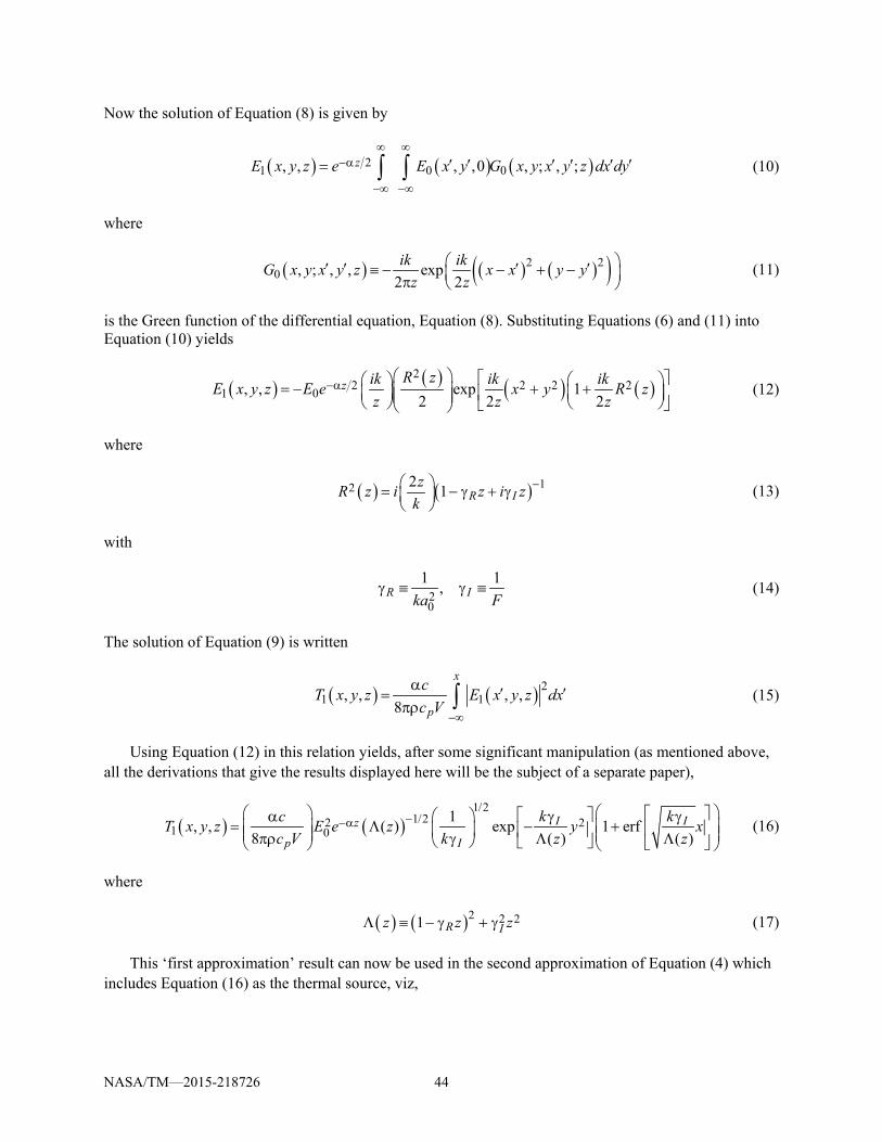
Now the solution of Equation (8) is given by

( ) ( ) ( )21 0 0, , , ,0 , ; , ;zE x y z e E x y G x y x y z dx dy∞ ∞

−α

−∞ −∞

′ ′ ′ ′ ′ ′= ∫ ∫ (10)

where

( ) ( ) ( )( )2 20 , ; , , exp

2 2ik ikG x y x y z x x y y

z z ′ ′ ′ ′≡ − − + − π

(11)

is the Green function of the differential equation, Equation (8). Substituting Equations (6) and (11) into Equation (10) yields

( ) ( ) ( ) ( )2

2 2 2 21 0, , exp 12 2 2

z R zik ik ikE x y z E e x y R zz z z

−α = − + + (12)

where

( ) ( ) 12 2 1 R IzR z i z i z

k− = − γ + γ

(13)

with

20

1 1,R Ika Fγ ≡ γ ≡ (14)

The solution of Equation (9) is written

( ) ( ) 21 1, , , ,

8

x

p

cT x y z E x y z dxc V

−∞

α ′ ′=πρ ∫ (15)

Using Equation (12) in this relation yields, after some significant manipulation (as mentioned above, all the derivations that give the results displayed here will be the subject of a separate paper),

( ) ( )1/2

1/22 21 01, , ( ) exp 1 erf

8 ( ) ( )I Iz

p I

c k kT x y z E e z y xc V k z z

−−α α γ γ

= Λ − + πρ γ Λ Λ (16)

where

( ) ( )2 2 21 R Iz z zΛ ≡ − γ + γ (17)

This ‘first approximation’ result can now be used in the second approximation of Equation (4) which includes Equation (16) as the thermal source, viz,

NASA/TM—2015-218726 44

2 22 2 1 22 2 2 T

E i kE E i T Ex k ⊥

∂ α− ∇ + = ε

∂ (18)

the solution of which can be written

( ) ( ) ( ) ( )22 0 0 10

, , , ,0 , ; , ; exp , ,2

zz T

ikE x y z e E x y G x y x y z T x y z dz∞ ∞

−α

−∞ −∞

′ ′ ′ ′ ′ ′= ε

∫ ∫ ∫ (19)

Using this second approximation expression, one can now obtain the behavior of the intensity of the propagating beam wave, of arbitrary initial radius and focal length, which includes the effects of thermal blooming within the atmosphere. From this, one can then immediately find expressions for the beam broadening and beam bending. Substituting Equations (6), (11), and (16) into Equation (19) gives for the beam wave intensity I(x,y,L) at a point (x,y) in a transverse plane at distance L downrange from the transmitter

( ) ( ) ( )( )

( ) ( )( ) ( ) ( )( )( )( ) ( ) ( )

22 2 2 2 2 2*2 0 1 1 2 2

2 2 2 21 1 2 2

2 21 1 2 2 1 1 2 21 2

( , , ) , , exp2 2

2 2

z k ikI x y L E x y L E e x y x yz

ik ikx x y y x x y yz z

i z x x z y y dx dy dx dy

∞ ∞ ∞ ∞−α

−∞ −∞ −∞ −∞

′ ′ ′ ′≡ = − Γ − −Γ − π

′ ′ ′ ′+ − + − − − + −

′ ′ ′ ′ ′ ′ ′ ′+ Φ − −Φ −

∫ ∫ ∫ ∫

(20)

where

( ) ( ) ( ) ( ) ( )5/22 22 21 2 9/22, ,

2R IR I

R II I

i z z z z kγ + γγ + γ π

Γ ≡ γ − γ Φ ≡ Ξ Φ ≡ Ξγ γ

(21)

and

( )20

2 2,2

T R

p R I

k Ez ze

c V−αη

ε γΞ ≡ α η ≡ ρ γ + γ

(22)

Again, leaving the details to a future publication, Equation (20) reduces to

( ) ( ) ( )( )( )( ) ( )

22 22 022 0 2 2( , , ) , , exp

L

x y x y

x x La e yI x y L E x y L Ea L a L a L a L

−α − ∆ ≡ = − −

(23)

where

( ) ( )0xa L a L≡ Λ (24)

is the radius along the x-axis of the beam at a distance z from the transmitter,

NASA/TM—2015-218726 45

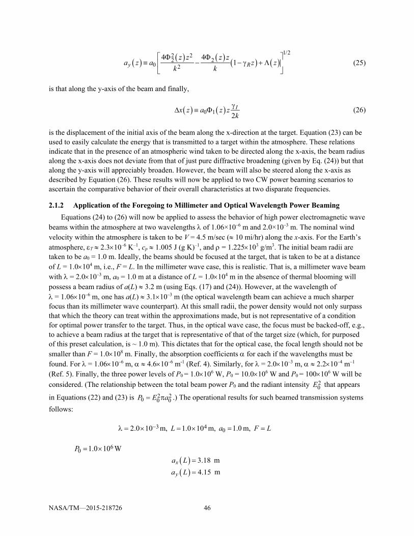
( ) ( ) ( ) ( ) ( )1/22 2

2 20 2

4 41y R

z z z za z a z z

k k Φ Φ

≡ − − γ + Λ

(25)

is that along the y-axis of the beam and finally,

( ) ( )0 1 2Ix z a z zkγ

∆ ≡ Φ (26)

is the displacement of the initial axis of the beam along the x-direction at the target. Equation (23) can be used to easily calculate the energy that is transmitted to a target within the atmosphere. These relations indicate that in the presence of an atmospheric wind taken to be directed along the x-axis, the beam radius along the x-axis does not deviate from that of just pure diffractive broadening (given by Eq. (24)) but that along the y-axis will appreciably broaden. However, the beam will also be steered along the x-axis as described by Equation (26). These results will now be applied to two CW power beaming scenarios to ascertain the comparative behavior of their overall characteristics at two disparate frequencies.

2.1.2 Application of the Foregoing to Millimeter and Optical Wavelength Power Beaming Equations (24) to (26) will now be applied to assess the behavior of high power electromagnetic wave

beams within the atmosphere at two wavelengths λ of 1.06×10–6 m and 2.0×10–3 m. The nominal wind velocity within the atmosphere is taken to be V = 4.5 m/sec (≈ 10 mi/hr) along the x-axis. For the Earth’s atmosphere, εT ≈ 2.3×10–6 K–1, cp ≈ 1.005 J (g K)–1, and ρ = 1.225×103 g/m3. The initial beam radii are taken to be a0 = 1.0 m. Ideally, the beams should be focused at the target, that is taken to be at a distance of L = 1.0×104 m, i.e., F = L. In the millimeter wave case, this is realistic. That is, a millimeter wave beam with λ = 2.0×10–3 m, a0 = 1.0 m at a distance of L = 1.0×104 m in the absence of thermal blooming will possess a beam radius of a(L) ≈ 3.2 m (using Eqs. (17) and (24)). However, at the wavelength of λ = 1.06×10–6 m, one has a(L) ≈ 3.1×10–3 m (the optical wavelength beam can achieve a much sharper focus than its millimeter wave counterpart). At this small radii, the power density would not only surpass that which the theory can treat within the approximations made, but is not representative of a condition for optimal power transfer to the target. Thus, in the optical wave case, the focus must be backed-off, e.g., to achieve a beam radius at the target that is representative of that of the target size (which, for purposed of this preset calculation, is ~ 1.0 m). This dictates that for the optical case, the focal length should not be smaller than F = 1.0×108 m. Finally, the absorption coefficients α for each if the wavelengths must be found. For λ = 1.06×10–6 m, α ≈ 4.6×10–6 m-1 (Ref. 4). Similarly, for λ = 2.0×10–3 m, α ≈ 2.2×10–4 m–1 (Ref. 5). Finally, the three power levels of P0 = 1.0×106 W, P0 = 10.0×106 W and P0 = 100×106 W will be considered. (The relationship between the total beam power P0 and the radiant intensity 2

0E that appears

in Equations (22) and (23) is 2 20 0 0P E a= π .) The operational results for such beamed transmission systems

follows: 32.0 10−λ = × m, 41.0 10L = × m, 0 1.0a = m, F L=

60 1.0 10 WP = × ( ) 3.18xa L = m ( ) 4.15ya L = m

NASA/TM—2015-218726 46

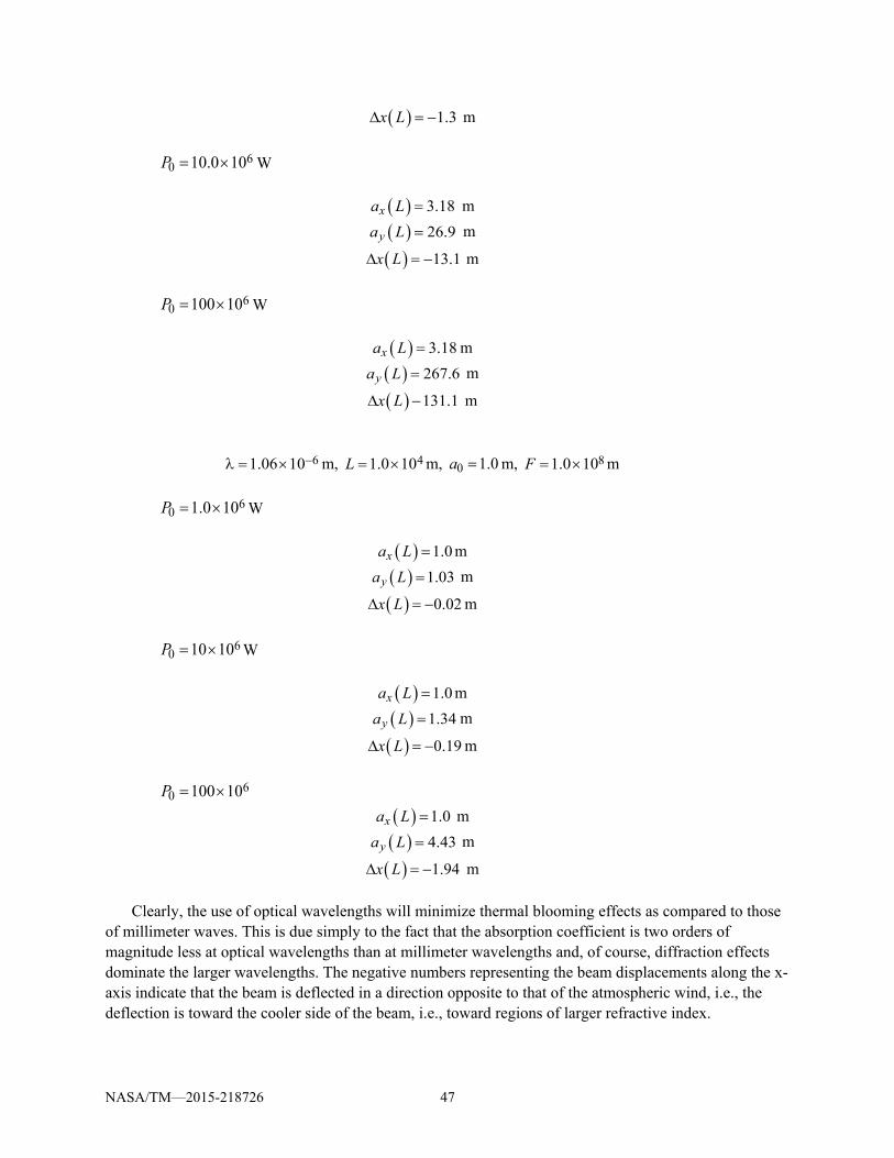
( ) 1.3x L∆ = − m

60 10.0 10P = × W

( ) 3.18xa L = m ( ) 26.9ya L = m

( ) 13.1x L∆ = − m

60 100 10P = × W

( ) 3.18xa L = m ( ) 267.6ya L = m

( ) 131.1x L∆ − m 61.06 10−λ = × m, 41.0 10L = × m, 0 1.0a = m, 81.0 10F = × m

60 1.0 10P = × W ( ) 1.0xa L = m ( ) 1.03ya L = m

( ) 0.02x L∆ = − m

60 10 10P = × W ( ) 1.0xa L = m ( ) 1.34ya L = m

( ) 0.19x L∆ = − m

60 100 10P = × ( ) 1.0xa L = m ( ) 4.43ya L = m

( ) 1.94x L∆ = − m

Clearly, the use of optical wavelengths will minimize thermal blooming effects as compared to those of millimeter waves. This is due simply to the fact that the absorption coefficient is two orders of magnitude less at optical wavelengths than at millimeter wavelengths and, of course, diffraction effects dominate the larger wavelengths. The negative numbers representing the beam displacements along the x-axis indicate that the beam is deflected in a direction opposite to that of the atmospheric wind, i.e., the deflection is toward the cooler side of the beam, i.e., toward regions of larger refractive index.

NASA/TM—2015-218726 47

The results of the analytical expressions derived here can also be displayed in various graphical formats. These will be included in the forthcoming publication that will detail the derivations of the equations. Equations (24) to (26) are, however, sufficient for use in the overall assessment of high-energy beam wave propagation within the atmosphere.

It also remains to subject a pulsed laser scenario to the same type of straightforward analysis as given above for the CW case. This will form the subject of another forthcoming paper. Also, atmospheric conditions have been assumed in which aerosols and such do not exist that may give rise to explosive detonation upon heating by the radiation field.

References

1. R. M. Manning, Stochastic Electromagnetic Image Propagation Through the Atmosphere, McGraw-Hill Book Co., New York, NY. 1993, Chapter 2.

2. A. D. Wheelon, Electromagnetic Scintillation: Volume 2, Weak Scattering, Cambridge University Press, 2003.

3. R. M. Manning, “High Energy Laser Beam Propagation and Thermal Blooming in the Atmosphere,” notes from an SPIE short course, Los Angeles, CA (1987).

4. E. P. Shettle and R. W. Fenn, “Models for the Aerosols of the Lower Atmosphere and Effects of Humidity Variations on Their Optical Properties,” Environmental Research Papers, No. 676, AFGL-TR-79-0214, Sept. 20, 1979.

5. H. J. Liebe and D. H. Layton, “Millimeter-Wave Properties of the Atmosphere: Laboratory Studies and Propagation Modeling,” NTIA Report 87-224, October, 1987.

NASA/TM—2015-218726 48