SL Note 96–38 (AP)

Beam Size, Emittance and Optical Functions in LEP

John M. Jowett

22 May 1996

Abstract

This note has a twofold purpose. The first is to discuss the physical princi-ples behind the estimation of emittance from beam size using measuring devices(such as the BEUV monitors) in LEP. This includes an explanation of some of thediscrepancies between “measured emittances” and the luminosity in LEP.

The second, closely related, purpose is more technical. The program MAD cal-culates a variety of functions describing the optics of LEP. The relation of beamsizes to emittance is used to illustrate the proper application of MAD’s capabili-ties and the meaning of the results. Some pitfalls in application of semi-intuitiverecipes are pointed out.

Most of the plots in this note are better viewed in colour. The note is also avail-able on the World-Wide-Web at:

http://hpariel.cern.ch/jowett/papers/beuvbeat/beuvbeat.html

Contents

1 Introduction 2

2 Calculations 32.1 The commands EMIT and ENVELOPE : : : : : : : : : : : : : : : : : : 32.2 The command TWISS : : : : : : : : : : : : : : : : : : : : : : : : : 5

3 Examples 53.1 An Imperfect LEP at 82 GeV : : : : : : : : : : : : : : : : : : : : : 63.2 Effect of a more symmetric RF system : : : : : : : : : : : : : : : : : 163.3 Perfect machine with symmetric RF : : : : : : : : : : : : : : : : : : 20

4 Conclusions 23

1

List of Figures

1 RF voltage distribution (imperfect ring) : : : : : : : : : : : : : : : : 62 Horizontal beam size (imperfect ring) : : : : : : : : : : : : : : : : : 73 Vertical beam size (imperfect ring) : : : : : : : : : : : : : : : : : : : 74 Horizontal �-beating (imperfect ring) : : : : : : : : : : : : : : : : : 95 Vertical �-beating (imperfect ring) : : : : : : : : : : : : : : : : : : : 96 Errors in horizontal beam size (imperfect ring) : : : : : : : : : : : : 107 Errors in vertical beam size (imperfect ring) : : : : : : : : : : : : : : 118 Horizontal dispersion (imperfect ring) : : : : : : : : : : : : : : : : : 129 Vertical dispersion (imperfect ring) : : : : : : : : : : : : : : : : : : 1210 Over-estimate of horizontal emittance (imperfect ring) : : : : : : : : 1311 Over-estimate of vertical emittance (imperfect ring) : : : : : : : : : : 1312 Beam tilt (imperfect ring) : : : : : : : : : : : : : : : : : : : : : : : 1413 Beam sizes at the IP (imperfect ring) : : : : : : : : : : : : : : : : : : 1514 Vertical beam size (symmetric RF) : : : : : : : : : : : : : : : : : : : 1615 Vertical �-beating (symmetric RF) : : : : : : : : : : : : : : : : : : : 1716 Vertical dispersion (symmetric RF) : : : : : : : : : : : : : : : : : : 1717 Beam tilt (symmetric RF) : : : : : : : : : : : : : : : : : : : : : : : 1818 Over-estimate of vertical emittance (symmetric RF) : : : : : : : : : : 1819 Beam sizes at the IP (symmetric RF) : : : : : : : : : : : : : : : : : : 1920 Horizontal beam size (perfect ring) : : : : : : : : : : : : : : : : : : 2021 Vertical �-beating (perfect ring) : : : : : : : : : : : : : : : : : : : : 2122 Horizontal dispersion (perfect ring) : : : : : : : : : : : : : : : : : : 2123 Beam sizes at the IP (perfect ring) : : : : : : : : : : : : : : : : : : : 22

List of Tables

1 Introduction

There are apparent inconsistencies between estimates of the LEP beam emittances fromdirect measurements via the BEUV monitors and the luminosity measured by the LEPexperiments. While LEP ran at the Z-resonance, these were not a serious concern asthe LEP experiments could measure luminosity rapidly and without any knowledge ofthe emittance. However the much smaller cross-sections at LEP2 energies will make itharder to measure luminosity directly and there will be a greater reliance on construct-ing the beam sizes at the IPs from the measured emittances.

As it has been shown that the discrepancies are unlikely to be instrumental [1], thecurrent view is that the discrepancy arises from poor knowledge of the beam optics atthe source point for the synchrotron light detected by the BEUV. In particular, it hasbeen shown [2] that better agreement can be obtained by using measured �-functionsand including the linear focusing perturbations due to the beam-beam interactions.

2

In this note1, I shall examine another aspect of the question, namely: is the usualdescription of the beam optics in terms of �- and dispersion functions adequate to de-scribe the relation

�x =q�x�x +Dx�2

" ; �y =q�y�y +Dy�2

" (1)

between the emittance and beam size? Given the strong energy-sawtoothing effects athigh energy, we might need to re-examine this relationship. In particular, we shouldreview how we get the values of �x;y and Dx;y and how much they depend on the (un-known) errors in the machine.

It has also been shown, in simulation [3], that it is possible, at least in principle, tomake the �-functions correspond more approximately to their theoretical values by amatching procedure involving the strengths of the interaction region quadrupoles. Thisrelies on the (generally valid) assumption that errors in these quadrupoles are the mainsource of “�-beating”.

This note contains no experimental data or discussion of the measurement deviceitself. It illustrates theoretical computations with numerical examples and examines theconsequences of different ways of extracting the emittance from the beam size. How-ever these have a direct bearing on how measurements—even those performed withperfect instrumentation—are interpreted.

Along the way, I have included a number of technical remarks footnotes which maybe useful to people doing optics calculations for LEP at high energy.

2 Calculations

Within MAD [4], there are various ways one might go about calculating the emittanceand beam size. The following is intended as a review for non-specialists. It sketchesthe physical meaning of the various methods with a minimum of formalism. Opticsafficionados are encouraged to jump straight to Section 3.

2.1 The commands EMIT and ENVELOPE

The recommended way is to use the command EMIT to calculate the emittances and thecommand ENVELOPE to calculate the beam sizes and correlation functions at selectedpoints around the ring. Let me make it clear that, to the best of our present knowledge,these commands correctly include all physical effects determining the emittance andbeam size in the context of linear single-particle dynamics including synchrotron radi-ation. I shall therefore use them as a reference and refer to the their results as the “true”beam sizes. “Errors” in other calculations of the beam size or emittance will be quotedwith respect to these values.

1This note expands and supersedes, but does not invalidate, preliminary calculations shown at theLEP Studies Working Group meeting of 30 April 1996. Those calculations used a crude method to gen-erate vertical emittance from betatron coupling. This note does it better.

3

If we could put a correct description of the real LEP into MAD, then we would wantfor nothing but these commands. Unfortunately, we do not know the imperfections ofthe real machine in sufficient detail and this is where the complications set in.

After finding the closed orbit (fixed point of the one-turn map from the starting az-imuth of the ring), MAD finds the eigenvectors of the tangent map and expresses themin terms of the primitive physical coordinates (x; px; y; py; t; pt) at the starting point ofthe ring [4]. These eigenvectors define the three normal modes of linear particle motionabout the closed orbit. Integrals around the ring [5] of the mean radiation power andthe two-point correlation function of its deviation from the mean (quantum fluctuation)projected into these modes give the radiation damping and diffusion rate from quantumexcitation. These are combined to give the emittances of the normal modes. The beamemittances are just the average values of the action variables for each normal mode.

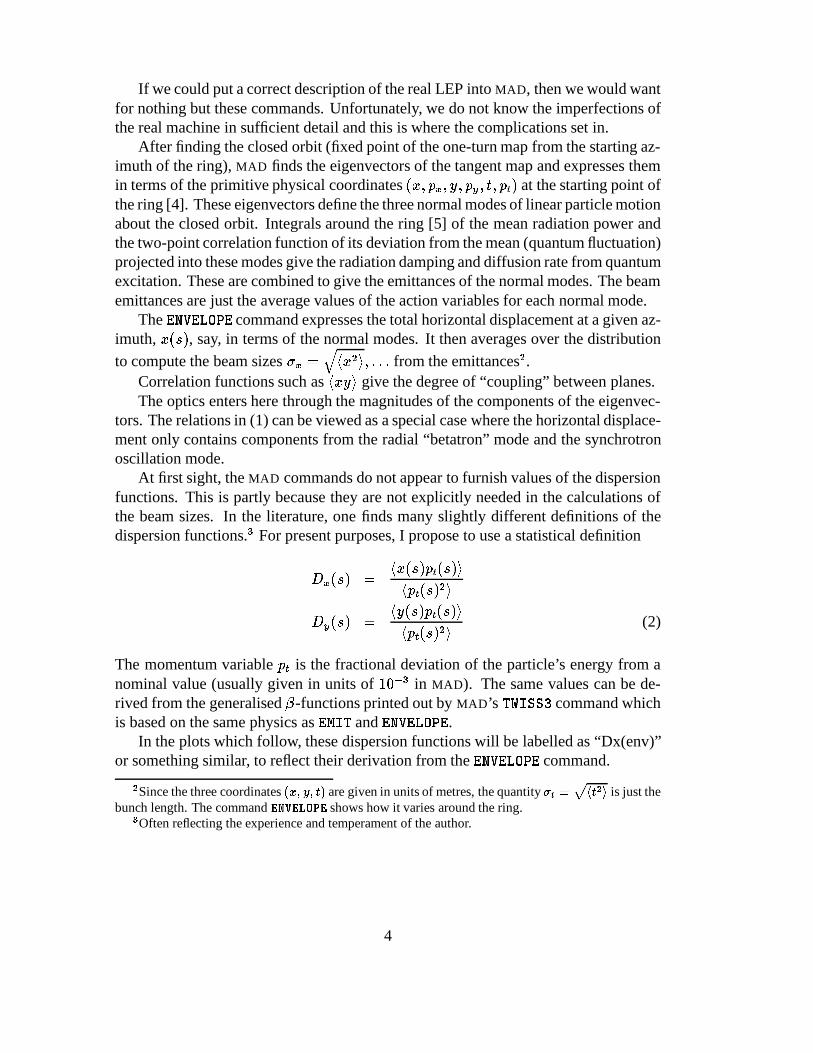
The ENVELOPE command expresses the total horizontal displacement at a given az-imuth, x(s), say, in terms of the normal modes. It then averages over the distribution

to compute the beam sizes �x =qhx2i; : : : from the emittances2.

Correlation functions such as hxyi give the degree of “coupling” between planes.The optics enters here through the magnitudes of the components of the eigenvec-

tors. The relations in (1) can be viewed as a special case where the horizontal displace-ment only contains components from the radial “betatron” mode and the synchrotronoscillation mode.

At first sight, the MAD commands do not appear to furnish values of the dispersionfunctions. This is partly because they are not explicitly needed in the calculations ofthe beam sizes. In the literature, one finds many slightly different definitions of thedispersion functions.3 For present purposes, I propose to use a statistical definition

Dx(s) =hx(s)pt(s)i

hpt(s)2i

Dy(s) =hy(s)pt(s)i

hpt(s)2i(2)

The momentum variable pt is the fractional deviation of the particle’s energy from anominal value (usually given in units of 10�3 in MAD). The same values can be de-rived from the generalised �-functions printed out by MAD’s TWISS3 command whichis based on the same physics as EMIT and ENVELOPE.

In the plots which follow, these dispersion functions will be labelled as “Dx(env)”or something similar, to reflect their derivation from the ENVELOPE command.

2Since the three coordinates (x; y; t) are given in units of metres, the quantity�t =p

ht2i is just thebunch length. The command ENVELOPE shows how it varies around the ring.

3Often reflecting the experience and temperament of the author.

4

2.2 The command TWISS

This command is much deprecated and much used, both with good reason. In the past,its main use was to calculate the Courant-Snyder or “Twiss” functions4 (including thedispersion function Dx), ignoring the effects of the RF and radiation. In the simplestversion of the command, the transverse betatron coupling is also ignored. This com-mand remains of use as a guide to matching new optics (particularly for hadron rings)but you have to be careful what you do with it. In operational practice, the Twiss func-tions needed in various applications have been taken from a table computed once andfor all for an ideal ring. Sometimes better results are obtained by using values measuredby the “1000 turns method”.

If the RF cavities and radiation are switched on in MAD, then TWISS will calcu-late Twiss functions taking them into account. In this case, it is well-known that the�-functions are good approximations to those calculated by TWISS3 but that the dis-persion functions are significantly wrong.

3 Examples

The following subsections treat a variety of cases, all based on this year’s nominal physicsoptics at 82 GeV. The optics is set up using the MAD commands:

call "/afs/cern.ch/user/s/slath/public/machines/lep96/lep966.seq"

call "/afs/cern.ch/user/s/slath/public/machines/lep96/dev/10860_physics.lep96"

Rather than give further detail here, let me say just say that you can find the files I usedin various sub-directories of:

/afs/cern.ch/users/j/jowett/public/lep96/beuvbeat/

In each case, the optics and beam parameters are calculated for both positrons and elec-trons. The results of the various MAD commands are dumped out into tables and com-pared and analysed in a spreadsheet environment.

For technical reasons, and because I want to make direct comparisons of e+e�, Ishow the values of optical functions at the beam position monitors (BPMs) and inter-action points, rather than at, say, the source points of the BEUV or other instruments5.

I used Version 8.19/3 of MAD.4If they are “Twiss”-anything, they are most definitely functions and not “Twiss parameters”.5To allow electrons to circulate in MAD, you have to reverse the sequence of machine elements (time-

reversal) and reflect the machine in a mirror to reverse all the magnetic fields (but not the electric fields).This is a consequence of a fundamental physical principle (non-CPT invariance when radiation is in-cluded). The BPMs and IPs are elements with zero length and have the agreeable property that, whenthe sequence is reversed, their entrances and exits are the same and they provide invariant observationpoints in all MAD commands. Indeed, some commands let you specify the centre or either end of anelement as an observation point. However not all of the commands I needed to use for this study areso obliging. In fact, the only one which offers this feature plus the further convenience of the SPLITcommand is OPTICS. OPTICS is physically equivalent to TWISS. The SPLIT command was introduced afew years ago precisely in order to allow observation points at the source points of instruments like theBEUV which lie inside magnets.

5

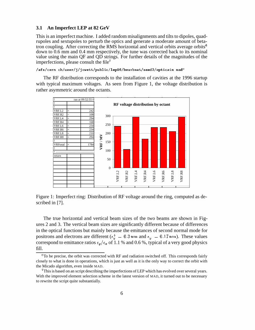
3.1 An Imperfect LEP at 82 GeV

This is an imperfect machine. I added random misalignments and tilts to dipoles, quad-rupoles and sextupoles to perturb the optics and generate a moderate amount of beta-tron coupling. After correcting the RMS horizontal and vertical orbits average orbits6down to 0.6 mm and 0.4 mm respectively, the tune was corrected back to its nominalvalue using the main QF and QD strings. For further details of the magnitudes of theimperfections, please consult the file7

/afs/cern.ch/user/j/jowett/public/lep96/beuvbeat/seed2/opticsim.mad"

The RF distribution corresponds to the installation of cavities at the 1996 startupwith typical maximum voltages. As seen from Figure 1, the voltage distribution israther asymmetric around the octants.

( p g )! ran at 09:52:55 07/05/96!!VRF.L2 = 242VRF.R2 = 108VRF.L4 = 294VRF.R4 = 168VRF.L6 = 234VRF.R6 = 234VRF.L8 = 210VRF.R8 = 294!VRFtotal = 1784!! ------------------------------------------------------------return

RF voltage distribution by octant

0

50

100

150

200

250

300V

RF

.L2

VR

F.R

2

VR

F.L

4

VR

F.R

4

VR

F.L

6

VR

F.R

6

VR

F.L

8

VR

F.R

8

VR

F /

MV

Figure 1: Imperfect ring: Distribution of RF voltage around the ring, computed as de-scribed in [7].

The true horizontal and vertical beam sizes of the two beams are shown in Fig-ures 2 and 3. The vertical beam sizes are significantly different because of differencesin the optical functions but mainly because the emittances of second normal mode forpositrons and electrons are different (�+y = 0:3 nm and ��y = 0:17 nm). These valuescorrespond to emittance ratios �y=�x of 1.1 % and 0.6 %, typical of a very good physicsfill.

6To be precise, the orbit was corrected with RF and radiation switched off. This corresponds fairlyclosely to what is done in operations, which is just as well as it is the only way to correct the orbit withthe Micado algorithm, even inside MAD.

7This is based on an script describing the imperfections of LEP which has evolved over several years.With the improved element selection scheme in the latest version of MAD, it turned out to be necessaryto rewrite the script quite substantially.

6

0

0.5

1

1.5

2

2.5

3

3.5

IP1

PU

.QD

22.R

1

PU

.QD

40.L

2

PU

.QS

10.L

2

PU

.QS

8.R

2

PU

.QD

36.R

2

PU

.QD

26.L

3

PU

.QL2

B.L

3

PU

.QL1

8.R

3

PU

.QD

44.L

4

PU

.QS

12.L

4

PU

.QS

6.R

4

PU

.QD

32.R

4

PU

.QD

30.L

5

PU

.QL5

.L5

PU

.QL1

6.R

5

PU

.QD

48.L

6

PU

.QS

15.L

6

PU

.QS

4.R

6

PU

.QD

28.R

6

PU

.QD

34.L

7

PU

.QL7

.L7

PU

.QL1

4.R

7

PU

.QD

46.R

7

PU

.QS

17.L

8

PU

.QS

1A.R

8

PU

.QD

24.R

8

PU

.QD

38.L

1

PU

.QL9

.L1

sigx

/ mm

envpos

envele

Figure 2: Imperfect ring: The true horizontal beam size (ENVELOPE command) at allthe BPMs and IPs around the ring for both e+ and e�.

0

0.05

0.1

0.15

0.2

0.25

0.3

0.35

0.4

0.45

IP1

PU

.QD

22.R

1

PU

.QD

40.L

2

PU

.QS

10.L

2

PU

.QS

8.R

2

PU

.QD

36.R

2

PU

.QD

26.L

3

PU

.QL2

B.L

3

PU

.QL1

8.R

3

PU

.QD

44.L

4

PU

.QS

12.L

4

PU

.QS

6.R

4

PU

.QD

32.R

4

PU

.QD

30.L

5

PU

.QL5

.L5

PU

.QL1

6.R

5

PU

.QD

48.L

6

PU

.QS

15.L

6

PU

.QS

4.R

6

PU

.QD

28.R

6

PU

.QD

34.L

7

PU

.QL7

.L7

PU

.QL1

4.R

7

PU

.QD

46.R

7

PU

.QS

17.L

8

PU

.QS

1A.R

8

PU

.QD

24.R

8

PU

.QD

38.L

1

PU

.QL9

.L1

sigy

/ mm

envpos

envele

Figure 3: Imperfect ring: The true vertical beam size (ENVELOPE command) at all theBPMs and IPs around the ring for both e+ and e�.

7

Figures 4 and 5 show the ratios of the �-functions calculated with and without ra-diation. The “�-beating due to radiation” is quite significant in the vertical mode anddifferent for the two beams.

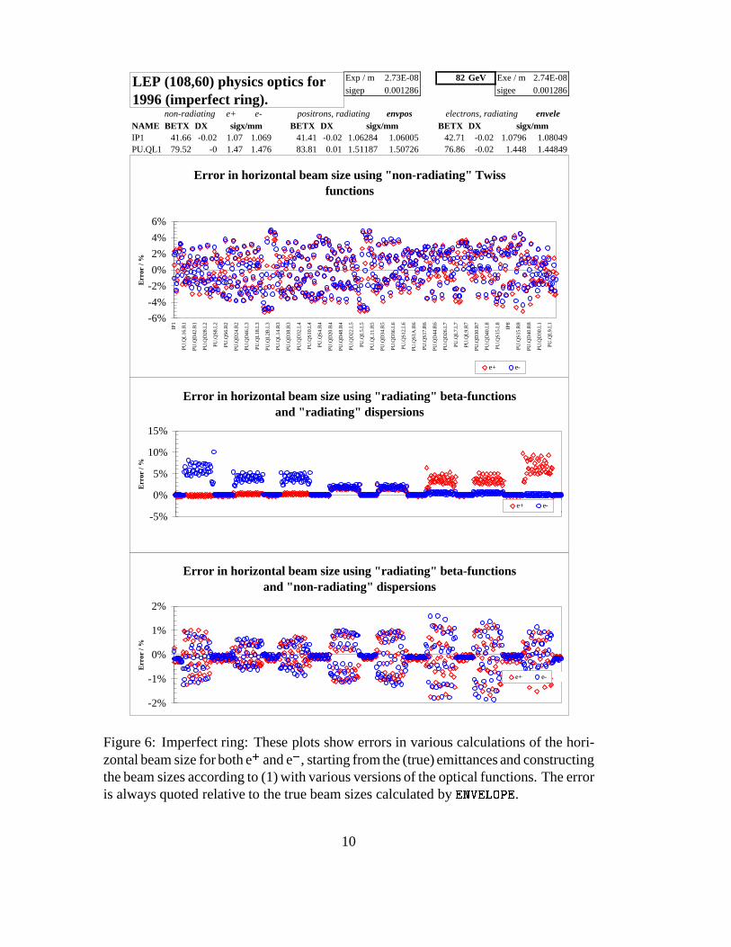
Figures 6 and 7 show the differences in beam sizes obtained by naive application offormulas like (1) with various versions of the optical functions. In each case a percent-age error relative to the true beam size is quoted. Except for the second case (wherethe dispersion function computed using the TWISS command with radiation is used),the results are reasonable in the horizontal plane. In the vertical plane the errors arelarge in all cases.

Figure 8 shows that the statistical definition, (2), of the horizontal dispersion func-tion is in rather good agreement with theDx obtained from theTWISS command withoutradiation and RF. On the other hand, Figure 9 shows that the statistical dispersion in thevertical plane is about a factor of two larger in this example.

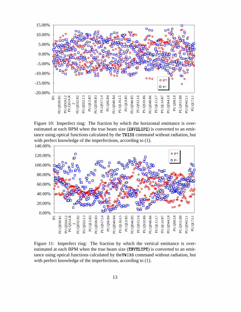
Figures 6 and 7 showed the error obtained by mis-predicting the beam size from aknowledge of the emittances. It is perhaps more important to consider the process ofestimating the emittance from knowledge of the beam sizes, e.g., at a device like theBEUV. For this purpose we can imagine that there is a device measuring the beam sizeat every BPM or IP and invert (1) to estimate the emittance (assuming knowledge of theenergy spread). Figures 10 and 11 shows the resulting error in the estimate of horizontaland vertical emittance. The error is very large in the vertical plane and could easilyexplain the observed discrepancy between the “measured vertical emittance” and theluminosity monitors8.

The main reason for the error in the naive calculation is the tilt of the beam profilesin configuration (x; y) space. This is characterised by the quantity

Rxy =hxyiqhx2i hy2i

(3)

which satisfies �1 � Rxy < 1. This quantity is plotted for the positrons in Figure 12.Despite what would normally be considered a very small global “coupling”, this quan-tity can take on rather large values locally.

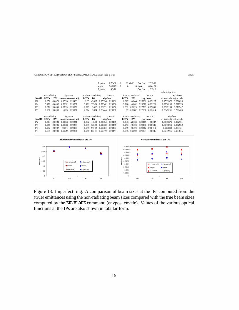
The effect of this on the estimation of beam sizes at the IPs is shown (somewhatindirectly) in Figure 13. Here the beam sizes at the IPs are reconstructed from knowl-edge of the true emittances in various ways. Although there is little scope for error inthe horizontal plane, the estimates of vertical beam sizes can vary quite widely. If onetakes into account that the vertical emittance being fed into such calculations could inpractice be a factor of two or so larger than the true one, it is easy to see that the verticalbeam size at the IPs could be over-estimated.

8This is not to deny the importance of other effects such as the perturbation of the optics by the beam-beam interaction.

8

0

0.2

0.4

0.6

0.8

1

1.2

IP1

PU

.QD

22.R

1

PU

.QD

40.L

2

PU

.QS

10.L

2

PU

.QS

8.R

2

PU

.QD

36.R

2

PU

.QD

26.L

3

PU

.QL2

B.L

3

PU

.QL1

8.R

3

PU

.QD

44.L

4

PU

.QS

12.L

4

PU

.QS

6.R

4

PU

.QD

32.R

4

PU

.QD

30.L

5

PU

.QL5

.L5

PU

.QL1

6.R

5

PU

.QD

48.L

6

PU

.QS

15.L

6

PU

.QS

4.R

6

PU

.QD

28.R

6

PU

.QD

34.L

7

PU

.QL7

.L7

PU

.QL1

4.R

7

PU

.QD

46.R

7

PU

.QS

17.L

8

PU

.QS

1A.R

8

PU

.QD

24.R

8

PU

.QD

38.L

1

PU

.QL9

.L1

beta

x(ra

d)/b

etax

(non

-rad

)

e+

e-

Figure 4: Imperfect ring: The ratio �radx =�non-rad

x for both e+ and e�. All calculationsinclude the same imperfections.

0

0.2

0.4

0.6

0.8

1

1.2

1.4

IP1

PU

.QD

22.R

1

PU

.QD

40.L

2

PU

.QS

10.L

2

PU

.QS

8.R

2

PU

.QD

36.R

2

PU

.QD

26.L

3

PU

.QL2

B.L

3

PU

.QL1

8.R

3

PU

.QD

44.L

4

PU

.QS

12.L

4

PU

.QS

6.R

4

PU

.QD

32.R

4

PU

.QD

30.L

5

PU

.QL5

.L5

PU

.QL1

6.R

5

PU

.QD

48.L

6

PU

.QS

15.L

6

PU

.QS

4.R

6

PU

.QD

28.R

6

PU

.QD

34.L

7

PU

.QL7

.L7

PU

.QL1

4.R

7

PU

.QD

46.R

7

PU

.QS

17.L

8

PU

.QS

1A.R

8

PU

.QD

24.R

8

PU

.QD

38.L

1

PU

.QL9

.L1

beta

y(ra

d)/b

etay

(non

-rad

)

e+

e-

Figure 5: Imperfect ring: The ratio �rady =�non�rad

y for both e+ and e�. All calculationsinclude the same imperfections.

9

Exp / m 2.73E-08 82 GeV Exe / m 2.74E-08sigep 0.001286 sigee 0.001286

non-radiating e+ e- positrons, radiating envpos electrons, radiating enveleNAME BETX DX sigx/mm BETX DX sigx/mm BETX DX sigx/mmIP1 41.66 -0.02 1.07 1.069 41.41 -0.02 1.06284 1.06005 42.71 -0.02 1.0796 1.08049PU.QL1B 79.52 -0 1.47 1.476 83.81 0.01 1.51187 1.50726 76.86 -0.02 1.448 1.44849PU.QL2B 123.5 -0 1.84 1.839 130.6 0.02 1.88711 1.88139 118.8 -0.02 1.8004 1.80082PU.QL4B 24 0.02 0.81 0.811 22.84 0.02 0.7897 0.788143 25.33 0.016 0.8313 0.831896PU.QL5 244.9 0.05 2.58 2.591 239.8 0.04 2.55774 2.55137 254 0.05 2.6328 2.63499PU.QL6 70.14 0.02 1.38 1.386 70.38 0.01 1.38552 1.38169 71.36 0.025 1.3954 1.39656PU.QL7 190.2 0.02 2.28 2.283 197.6 0 2.32153 2.31454 187.3 0.036 2.2603 2.26166PU.QL8 57.81 0 1.26 1.258 61.37 -0.01 1.29376 1.28984 55.46 0.016 1.23 1.23041PU.QL9 126.3 -0.01 1.86 1.86 135.4 -0.04 1.9222 1.91682 118.8 0.015 1.8 1.79971PU.QL10 43.08 -0.02 1.08 1.087 45.56 -0.03 1.11546 1.11288 40.66 0.002 1.0531 1.05253PU.QL1 121.4 -0.04 1.82 1.824 123.1 -0.07 1.83434 1.83128 118.5 -0.01 1.7977 1.7966PU.QL12 45.12 -0.02 1.11 1.112 43.61 -0.03 1.09151 1.09012 46 -0.01 1.1201 1.11965PU.QL14 9.639 0.28 0.63 0.629 9.697 0.28 0.63053 0.629599 9.775 0.228 0.594 0.627883PU.QL15 88.86 0.98 2.01 2.009 91.74 1.01 2.04283 2.04583 85.5 0.789 1.8332 1.96157PU.QL16 31.44 0.53 1.15 1.153 30.44 0.54 1.14837 1.15033 32.02 0.427 1.0837 1.1478PU.QL17 122.2 0.91 2.17 2.174 114.2 0.93 2.13111 2.13289 129.4 0.739 2.1053 2.20591PU.QL1 30.62 0.45 1.08 1.081 29.58 0.45 1.06788 1.06678 32.02 0.367 1.0469 1.09746PU.QD2 11.98 0.41 0.78 0.782 12.07 0.41 0.77605 0.773005 11.76 0.348 0.7216 0.785075PU.QD2 25.2 0.41 0.98 0.985 25.67 0.41 0.991 0.989405 25.26 0.334 0.9346 0.980709PU.QD2 19.44 0.43 0.92 0.917 18.22 0.44 0.90299 0.903918 20.52 0.351 0.8735 0.927567PU.QD2 16.42 0.43 0.87 0.867 17.51 0.42 0.87848 0.875251 15.59 0.359 0.7989 0.860672PU.QD2 26.49 0.41 1 1.001 25.51 0.41 0.98375 0.981658 27.78 0.336 0.972 1.01737PU.QD3 13.09 0.42 0.81 0.809 13.17 0.43 0.81589 0.817538 12.84 0.34 0.736 0.795523PU.QD3 23.68 0.43 0.98 0.976 24.19 0.43 0.9809 0.978474 23.68 0.357 0.9255 0.979214PU.QD3 19.23 0.41 0.9 0.897 18.02 0.4 0.87243 0.869984 20.33 0.342 0.865 0.917215PU.QD3 16.43 0.42 0.86 0.86 17.53 0.42 0.8805 0.880753 15.55 0.337 0.7822 0.837422PU.QD3 24.92 0.43 0.99 0.995 24.07 0.43 0.98382 0.983061 26.03 0.354 0.9575 1.00852PU.QD4 13.84 0.42 0.82 0.816 13.92 0.41 0.81041 0.807466 13.61 0.35 0.7574 0.819037PU.QD4 23.4 0.42 0.96 0.963 23.92 0.42 0.97029 0.969022 23.36 0.338 0.9089 0.957575PU.QD4 19 0.43 0.91 0.911 17.84 0.44 0.89735 0.89853 20.02 0.35 0.8651 0.919625PU.QD4 16.1 0.42 0.86 0.857 17.23 0.42 0.86904 0.86572 15.2 0.353 0.7876 0.848068PU.QD4 25.04 0.41 0.98 0.982 24.07 0.41 0.96467 0.962639 26.27 0.338 0.9515 0.9982PU.QD4 14.1 0.43 0.83 0.832 14.18 0.44 0.83914 0.840719 13.86 0.346 0.7588 0.818518PU.QD4 22.56 0.43 0.96 0.959 23.13 0.43 0.96465 0.962241 22.45 0.355 0.9057 0.95979PU.QD4 19.56 0.41 0.9 0.901 18.29 0.4 0.87544 0.873211 20.71 0.341 0.87 0.921672PU.QD4 15.8 0.42 0.85 0.853 16.98 0.43 0.87537 0.875601 14.83 0.34 0.7716 0.828415PU.QD4 24.74 0.43 0.99 0.993 23.81 0.43 0.98079 0.980424 25.88 0.354 0.9553 1.00685PU.QD3 14.4 0.41 0.82 0.823 14.44 0.41 0.81673 0.813898 14.25 0.347 0.7665 0.826562PU.QD3 21.91 0.42 0.94 0.941 22.5 0.42 0.95002 0.949081 21.73 0.337 0.8835 0.933508PU.QD3 20.07 0.43 0.92 0.926 18.76 0.44 0.91072 0.912288 21.24 0.35 0.884 0.938003PU.QD3 15.68 0.42 0.85 0.85 16.91 0.42 0.8644 0.861197 14.67 0.352 0.7782 0.83936PU.QD3 24.34 0.41 0.97 0.973 23.36 0.41 0.95639 0.955252 25.51 0.338 0.9404 0.988427PU.QD2 14.89 0.43 0.84 0.842 14.94 0.43 0.84794 0.849685 14.74 0.344 0.7727 0.830942PU.QD2 20.04 0.42 0.92 0.918 20.74 0.42 0.92598 0.923745 19.67 0.35 0.8597 0.915126PU.QD2 21 0.41 0.92 0.922 19.55 0.4 0.89565 0.894212 22.35 0.339 0.8941 0.944646PU.QD2 15.56 0.43 0.85 0.855 16.85 0.44 0.87943 0.87989 14.45 0.347 0.7702 0.82948PU.QD2 22.5 0.43 0.96 0.959 21.59 0.43 0.9462 0.946168 23.52 0.351 0.9194 0.97232PU.QS18 16.25 0.4 0.84 0.846 16.23 0.4 0.84022 0.837547 16.26 0.337 0.7948 0.849977PU.QS17 112.7 0.65 1.94 1.947 104.6 0.64 1.88145 1.87928 120.9 0.539 1.9436 2.00492PU.QS16 80.71 0.48 1.61 1.611 76.61 0.48 1.57052 1.56879 85.26 0.397 1.608 1.64877

Error in horizontal beam size using "non-radiating" Twiss functions

-6%

-4%

-2%

0%

2%

4%

6%

IP1

PU

.QL1

6.R

1

PU

.QD

42.R

1

PU

.QD

28.L

2

PU

.QS

8.L2

PU

.QS

6.R

2

PU

.QD

24.R

2

PU

.QD

46.L

3

PU

.QL1

8.L3

PU

.QL2

B.L

3

PU

.QL1

4.R

3

PU

.QD

38.R

3

PU

.QD

32.L

4

PU

.QS

10.L

4

PU

.QS

4.R

4

PU

.QD

20.R

4

PU

.QD

48.R

4

PU

.QD

22.L

5

PU

.QL5

.L5

PU

.QL1

1.R

5

PU

.QD

34.R

5

PU

.QD

36.L

6

PU

.QS

12.L

6

PU

.QS

1A.R

6

PU

.QS

17.R

6

PU

.QD

44.R

6

PU

.QD

26.L

7

PU

.QL7

.L7

PU

.QL9

.R7

PU

.QD

30.R

7

PU

.QD

40.L

8

PU

.QS

15.L

8

IP8

PU

.QS

15.R

8

PU

.QD

40.R

8

PU

.QD

30.L

1

PU

.QL9

.L1

Err

or /

%

e+ e-

Error in horizontal beam size using "radiating" beta-functions and "non-radiating" dispersions

-2%

-1%

0%

1%

2%

Err

or /

%

e+ e-

Error in horizontal beam size using "radiating" beta-functions and "radiating" dispersions

-5%

0%

5%

10%

15%

Err

or /

%

e+ e-

LEP (108,60) physics optics for 1996 (imperfect ring).

Figure 6: Imperfect ring: These plots show errors in various calculations of the hori-zontal beam size for both e+ and e�, starting from the (true) emittances and constructingthe beam sizes according to (1) with various versions of the optical functions. The erroris always quoted relative to the true beam sizes calculated by ENVELOPE.

10

Eyp / m 3.01E-10 82 GeV Eye / m 1.7E-10sigep 0.001286 sigee 0.00129

1.10% 0.60%non-radiating e+ e- positrons, radiating envpos electrons, radiating envele

NAME BETY DY sigy/mm BETY DY sigy/mm BETY DY sigy/mmIP1 27.66 0.009 0.091 0.069 25.02 0.01 0.0868 0.112439 30.22 0.01 0.0706 0.09399PU.QL1B 31.78 -0.004 0.098 0.073 34.35 -0.01 0.1017 0.133666 29.76 2E-04 0.0701 0.10228PU.QL2B 18.78 -0.007 0.075 0.056 21.09 -0.01 0.0797 0.103666 16.94 -0 0.0529 0.07754PU.QL4B 129.1 -0.035 0.197 0.153 133 -0.04 0.2001 0.25051 127.9 -0.03 0.1453 0.19446PU.QL5 8.413 -0.009 0.05 0.039 7.562 -0.01 0.0477 0.060317 9.275 -0.01 0.0391 0.05048PU.QL6 79.22 0.013 0.154 0.116 88.74 0.02 0.1635 0.211069 71.68 0.006 0.1088 0.15818PU.QL7 22.26 0.015 0.082 0.064 23.53 0.02 0.0842 0.106031 21.56 0.011 0.0597 0.08091PU.QL8 70.84 0.029 0.146 0.115 64.51 0.03 0.1394 0.176884 77.47 0.025 0.1131 0.14689PU.QL9 13.37 0.006 0.063 0.048 12.67 0 0.0618 0.081131 14.04 0.007 0.0481 0.06653PU.QL10 65.91 -0.015 0.141 0.106 74.04 -0.02 0.1493 0.192131 59.53 -0.01 0.0991 0.14347PU.QL1 22.36 -0.016 0.082 0.064 23.49 -0.02 0.0841 0.106001 21.81 -0.010.06 0.08115PU.QL12 80.27 -0.031 0.155 0.122 72.47 -0.03 0.1477 0.187754 88.28 -0.03 0.1207 0.15663PU.QL14 138.8 -0.014 0.204 0.152 137.2 -0 0.2032 0.265956 140.6 -0.02 0.1524 0.21353PU.QL15 43.88 2E-04 0.115 0.085 46.79 0.01 0.1187 0.154525 41.52 -0 0.0828 0.11914PU.QL16 129.9 0.016 0.198 0.148 145.6 0.03 0.2094 0.269359 117.4 0.008 0.1392 0.20119PU.QL17 8.55 0.01 0.051 0.04 8.726 0.01 0.0513 0.064408 8.575 0.008 0.0376 0.05009PU.QL1 134.6 0.014 0.201 0.15 132.1 0 0.1994 0.260635 137.1 0.017 0.1505 0.21005PU.QD2 168.6 -0.032 0.225 0.172 188.1 -0.04 0.238 0.300901 154.2 -0.02 0.1596 0.22369PU.QD2 173.2 -0.044 0.228 0.178 159.2 -0.05 0.2189 0.277028 188.8 -0.04 0.1765 0.22997PU.QD2 139.3 -0.014 0.205 0.153 137.4 -0 0.2034 0.267253 141.4 -0.02 0.1528 0.21575PU.QD2 170.6 0.03 0.227 0.172 190.8 0.04 0.2397 0.299803 155.9 0.019 0.1604 0.22057PU.QD2 172.1 0.048 0.228 0.18 158.1 0.05 0.2182 0.274716 187.7 0.04 0.176 0.22727PU.QD3 141.9 0.02 0.207 0.155 139.6 0.01 0.205 0.266488 144.5 0.022 0.1545 0.21463PU.QD3 168 -0.028 0.225 0.171 188.3 -0.04 0.2381 0.297213 153.1 -0.02 0.159 0.21767PU.QD3 166.7 -0.048 0.224 0.177 152.7 -0.05 0.2144 0.270208 182 -0.04 0.1733 0.22388PU.QD3 145.9 -0.02 0.21 0.157 144.5 -0.01 0.2086 0.270647 147.9 -0.02 0.1562 0.21678PU.QD3 168.1 0.028 0.225 0.17 188.4 0.04 0.2382 0.29708 153.2 0.017 0.159 0.21696PU.QD4 165.6 0.054 0.223 0.179 152.2 0.06 0.2141 0.271002 180.2 0.045 0.1725 0.22162PU.QD4 147.2 0.028 0.211 0.16 145.5 0.02 0.2093 0.274295 149.2 0.03 0.157 0.22099PU.QD4 167.6 -0.024 0.225 0.169 187.7 -0.04 0.2377 0.295602 152.8 -0.01 0.1588 0.21586PU.QD4 165.3 -0.058 0.223 0.181 152.9 -0.06 0.2146 0.275546 178.8 -0.05 0.1718 0.22386PU.QD4 145.4 -0.034 0.209 0.161 143.6 -0.02 0.2079 0.278256 147.3 -0.03 0.156 0.2266PU.QD4 170 0.023 0.226 0.17 189.7 0.04 0.239 0.296936 155.8 0.013 0.1604 0.2178PU.QD4 166.5 0.055 0.224 0.18 155.4 0.06 0.2163 0.274165 178.6 0.045 0.1717 0.22054PU.QD4 144.2 0.031 0.208 0.159 141.6 0.02 0.2065 0.273109 146.3 0.031 0.1554 0.22134PU.QD4 170.6 -0.025 0.227 0.171 189.4 -0.04 0.2388 0.296182 157.2 -0.01 0.1611 0.21751PU.QD4 165.7 -0.048 0.223 0.177 156 -0.05 0.2168 0.265544 176.2 -0.04 0.1706 0.20925PU.QD3 145.4 -0.021 0.209 0.157 142.2 -0.01 0.2069 0.267542 147.5 -0.02 0.1561 0.21392PU.QD3 169.2 0.027 0.226 0.171 186.6 0.04 0.2371 0.292806 156.9 0.017 0.161 0.21484PU.QD3 167.5 0.042 0.225 0.175 159.6 0.05 0.2192 0.262321 176.4 0.034 0.1706 0.20238PU.QD3 145.8 0.012 0.21 0.156 141.6 0 0.2065 0.264921 148.3 0.015 0.1565 0.21121PU.QD3 166.7 -0.032 0.224 0.171 182.5 -0.04 0.2345 0.288966 155.9 -0.02 0.1604 0.21138PU.QD2 170.8 -0.039 0.227 0.175 165 -0.04 0.2229 0.263684 177.7 -0.03 0.1713 0.19942PU.QD2 140.8 -0.008 0.206 0.153 136.3 0 0.2026 0.26787 142.8 -0.01 0.1536 0.21814PU.QD2 170.9 0.034 0.227 0.173 185.5 0.05 0.2363 0.290247 161.5 0.022 0.1633 0.21323PU.QD2 175.6 0.045 0.23 0.18 172.6 0.05 0.228 0.271072 180.1 0.036 0.1724 0.20211PU.QD2 137.4 0.007 0.203 0.151 131.9 -0 0.1993 0.254737 139.8 0.011 0.1519 0.20555PU.QS18 170.8 -0.039 0.227 0.175 183.5 -0.05 0.2351 0.292524 163.3 -0.03 0.1642 0.21645PU.QS17 56.59 -0.026 0.131 0.102 60.51 -0.03 0.135 0.163924 54.56 -0.02 0.0949 0.11777PU.QS16 97.56 -0.035 0.171 0.135 100.7 -0.04 0.1741 0.207378 96.56 -0.03 0.1263 0.14884

Error in vertical beam size using "non-radiating" Twiss functions

-35%-30%-25%-20%-15%-10%-5%0%

IP1

PU

.QL1

6.R

1

PU

.QD

42.R

1

PU

.QD

28.L

2

PU

.QS

8.L2

PU

.QS

6.R

2

PU

.QD

24.R

2

PU

.QD

46.L

3

PU

.QL1

8.L3

PU

.QL2

B.L

3

PU

.QL1

4.R

3

PU

.QD

38.R

3

PU

.QD

32.L

4

PU

.QS

10.L

4

PU

.QS

4.R

4

PU

.QD

20.R

4

PU

.QD

48.R

4

PU

.QD

22.L

5

PU

.QL5

.L5

PU

.QL1

1.R

5

PU

.QD

34.R

5

PU

.QD

36.L

6

PU

.QS

12.L

6

PU

.QS

1A.R

6

PU

.QS

17.R

6

PU

.QD

44.R

6

PU

.QD

26.L

7

PU

.QL7

.L7

PU

.QL9

.R7

PU

.QD

30.R

7

PU

.QD

40.L

8

PU

.QS

15.L

8

IP8

PU

.QS

15.R

8

PU

.QD

40.R

8

PU

.QD

30.L

1

PU

.QL9

.L1

Err

or /

%

e+ e-

Error in vertical beam size using "radiating" beta-functions and "non-radiating" dispersions

-40%

-30%

-20%

-10%

0%

Err

or /

%

e+ e-

Error in vertical beam size using "radiating" beta-functions and "radiating" dispersions

-40%

-30%

-20%

-10%

0%

Err

or /

%

e+ e-

LEP (108,60) physics optics for 1996 (imperfect ring).

Figure 7: Imperfect ring: These plots show errors in various calculations of the verticalbeam size for both e+ and e�, starting from the (true) emittances and constructing thebeam sizes according to (1) with various versions of the optical functions. The error isalways quoted relative to the true beam sizes calculated by ENVELOPE.

11

-0.1

0.1

0.3

0.5

0.7

0.9

1.1

IP1

PU.QD28.R1

PU.QD28.L2

PU.QS0.L2

PU.QD24.R2

PU.QD32.L3

PU.QL2B.L3

PU.QD24.R3

PU.QD32.L4

PU.QS3.L4

PU.QD20.R4

PU.QD36.L5

PU.QL5.L5

PU.QD20.R5

PU.QD36.L6

PU.QS5.L6

PU.QS17.R6

PU.QD40.L7

PU.QL7.L7

PU.QL17.R7

PU.QD40.L8

PU.QS7.L8

PU.QS15.R8

PU.QD44.L1

PU.QL9.L1

D x / mD

X

Dx(env)

Figure8:

Imperfect

ring:H

orizontaldispersion

functionfor

positronscalculated

bythe

TWISS

comm

andw

ithoutradiationcom

paredw

iththatderived

fromthe

ENVELOPE

comm

andusing

(2).

-0.2

-0.15

-0.1

-0.05 0

0.0

5

0.1

0.1

5

0.2

IP1

PU.QD30.R1

PU.QD24.L2PU.QS1A.R

2PU.QD32.R2

PU.QD22.L3

PU.QL5.R3

PU.QD38.R3

PU.QS17.L4

PU.QS6.R4

PU.QD40.R4

PU.QL16.L5

PU.QL9.R5

PU.QD46.R5

PU.QS12.L6

PU.QS10.R6

PU.QD48.R6

PU.QL11.L7

PU.QL14.R7

PU.QD44.L8

PU.QS8.L8

PU.QS15.R8

PU.QD42.L1

PU.QL7.L1

D y / m

DY

Dy(env)

Figure9:

Imperfectring:

Vertical

dispersionfunction

forpositrons

calculatedby

theTWISS

comm

andw

ithoutradiation

compared

with

thatderived

fromthe

ENVELOPE

comm

andusing

(2).

12

-20.00%

-15.00%

-10.00%

-5.00%

0.00%

5.00%

10.00%

15.00%

IP1

PU

.QD

30.R

1

PU

.QD

24.L

2P

U.Q

S1A

.R2

PU

.QD

32.R

2

PU

.QD

22.L

3

PU

.QL5

.R3

PU

.QD

38.R

3

PU

.QS

17.L

4

PU

.QS

6.R

4

PU

.QD

40.R

4

PU

.QL1

6.L5

PU

.QL9

.R5

PU

.QD

46.R

5

PU

.QS

12.L

6

PU

.QS

10.R

6

PU

.QD

48.R

6

PU

.QL1

1.L7

PU

.QL1

4.R

7

PU

.QD

44.L

8

PU

.QS

8.L8

PU

.QS

15.R

8

PU

.QD

42.L

1

PU

.QL7

.L1

e+

e-

Figure 10: Imperfect ring: The fraction by which the horizontal emittance is over-estimated at each BPM when the true beam size (ENVELOPE) is converted to an emit-tance using optical functions calculated by the TWISS command without radiation, butwith perfect knowledge of the imperfections, according to (1).

0.00%

20.00%

40.00%

60.00%

80.00%

100.00%

120.00%

140.00%

IP1

PU

.QD

30.R

1

PU

.QD

24.L

2P

U.Q

S1A

.R2

PU

.QD

32.R

2

PU

.QD

22.L

3

PU

.QL5

.R3

PU

.QD

38.R

3

PU

.QS

17.L

4

PU

.QS

6.R

4

PU

.QD

40.R

4

PU

.QL1

6.L5

PU

.QL9

.R5

PU

.QD

46.R

5

PU

.QS

12.L

6

PU

.QS

10.R

6

PU

.QD

48.R

6

PU

.QL1

1.L7

PU

.QL1

4.R

7

PU

.QD

44.L

8

PU

.QS

8.L8

PU

.QS

15.R

8

PU

.QD

42.L

1

PU

.QL7

.L1

e+

e-

Figure 11: Imperfect ring: The fraction by which the vertical emittance is over-estimated at each BPM when the true beam size (ENVELOPE) is converted to an emit-tance using optical functions calculated by theTWISS command without radiation, butwith perfect knowledge of the imperfections, according to (1).

13

-0.6

-0.4

-0.2 0

0.2

0.4

0.6

IP1

D28.R1

QD28.L2

QS0.L2

D24.R2

QD32.L3

L2B.L3

D24.R3

QD32.L4

QS3.L4

D20.R4

QD36.L5

QL5.L5

D20.R5

QD36.L6

QS5.L6

QS17.R6

QD40.L7

QL7.L7

QL17.R7

QD40.L8

QS7.L8

QS15.R8

QD44.L1

QL9.L1

R(x,y)+

Figure12:

Imperfectring:

The

beamtiltforpositrons

computed

bythe

ENVELOPE

com-

mand

inM

AD

.

14

G:\HOME\JOWETT\LEP96\BEUVBEAT\SEED2\OPTICSIN.XLS[Beam sizes at IPs] 23:25 2

Exp / m 2.7E-08 0 82 GeV Exe / m 2.7E-08sigep 0.00129 0 0 0 sigee 0.00129Eyp / m 3E-10 Eye / m 1.7E-10

mixed functionsnon-radiating sigx/mm positrons, radiating envpos electrons, radiating envele sigx / mm

NAME BETX DX + (non-ra- (non-rad) BETX DX sigx/mm BETX DX sigx/mm e+ (mixed) e- (mixed)IP2 2.352 -0.0073 0.2535 0.25403 2.35 -0.007 0.25336 0.25331 2.327 -0.006 0.25201 0.25227 0.2533572 0.252626IP4 3.196 -0.0002 0.2952 0.29587 3.161 7E-04 0.29362 0.29366 3.228 -0.002 0.29672 0.29723 0.2936233 0.297373IP6 2.872 0.0031 0.2799 0.28052 2.909 0.003 0.28171 0.28156 2.832 0.0029 0.27793 0.27833 0.2817159 0.278547IP8 1.937 0.0065 0.23 0.23051 2.014 0.004 0.23444 0.23388 1.87 0.0082 0.22608 0.22614 0.2345251 0.226489

non-radiating sigy/mm positrons, radiating envpos electrons, radiating envele sigy/mmNAME BETY DY + (non-ra- (non-rad) BETY DY sigy/mm BETY DY sigy/mm e+ (mixed) e- (mixed)IP2 0.044 -0.0002 0.0036 0.00271 0.042 -1E-04 0.00354 0.00445 0.046 -2E-04 0.00275 0.0037 0.0035371 0.002751IP4 0.048 -0.0005 0.0038 0.00288 0.045 -6E-04 0.00369 0.00459 0.053 -4E-04 0.00296 0.00385 0.0036911 0.002962IP6 0.052 -0.0007 0.004 0.00306 0.049 -9E-04 0.00384 0.00493 0.059 -5E-04 0.00312 0.00413 0.003838 0.003121IP8 0.051 0.0001 0.0039 0.00291 0.048 -8E-05 0.00379 0.00444 0.056 0.0002 0.00304 0.0036 0.0037915 0.003035

Horizontal beam sizes at the IPs

0

0.05

0.1

0.15

0.2

0.25

0.3

IP2 IP4 IP6 IP8

sigx

/ m

m

e+ (non-rad) e- (non-rad)

envpos envele

e+ (mixed) e- (mixed)

Vertical beam sizes at the IPs

0

0.0005

0.001

0.0015

0.002

0.0025

0.003

0.0035

0.004

0.0045

0.005

IP2 IP4 IP6 IP8

sigx

/ m

m

e+ (non-rad) e- (non-rad)

envpos envele

e+ (mixed) e- (mixed)

Figure 13: Imperfect ring: A comparison of beam sizes at the IPs computed from the(true) emittances using the non-radiating beam sizes compared with the true beam sizescomputed by the ENVELOPE command (envpos, envele). Values of the various opticalfunctions at the IPs are also shown in tabular form.

15

3.2 Effect of a more symmetric RF system

It might be suggested that some of the effects seen in the above example are related tothe asymmetry of the RF voltage distribution [6]. To see how much can be attributed toRF asymmetry, I repeated the same calculations with exactly the same machine imper-fections but with an RF system adjusted to provide equal voltage in each octant. Thismeant that certain superconducting RF units were given voltages much higher than theyare capable of in reality. The total RF voltage was kept the same as in the exampleof Section 3.1. The analogous plot to Figure 1 would show eight equal bars of height222 MV.

Figure 14 shows that symnmstrizing the RF does not get rid of the difference invertical beam sizes.

0

0.05

0.1

0.15

0.2

0.25

0.3

0.35

0.4

IP1

PU

.QD

22.R

1

PU

.QD

40.L

2

PU

.QS

10.L

2

PU

.QS

8.R

2

PU

.QD

36.R

2

PU

.QD

26.L

3

PU

.QL2

B.L

3

PU

.QL1

8.R

3

PU

.QD

44.L

4

PU

.QS

12.L

4

PU

.QS

6.R

4

PU

.QD

32.R

4

PU

.QD

30.L

5

PU

.QL5

.L5

PU

.QL1

6.R

5

PU

.QD

48.L

6

PU

.QS

15.L

6

PU

.QS

4.R

6

PU

.QD

28.R

6

PU

.QD

34.L

7

PU

.QL7

.L7

PU

.QL1

4.R

7

PU

.QD

46.R

7

PU

.QS

17.L

8

PU

.QS

1A.R

8

PU

.QD

24.R

8

PU

.QD

38.L

1

PU

.QL9

.L1

sigy

/ mm

envpos

envele

Figure 14: Imperfect ring with symmetric RF: The true vertical beam size (ENVELOPEcommand) at all the BPMs and IPs around the ring for both e+ and e�.

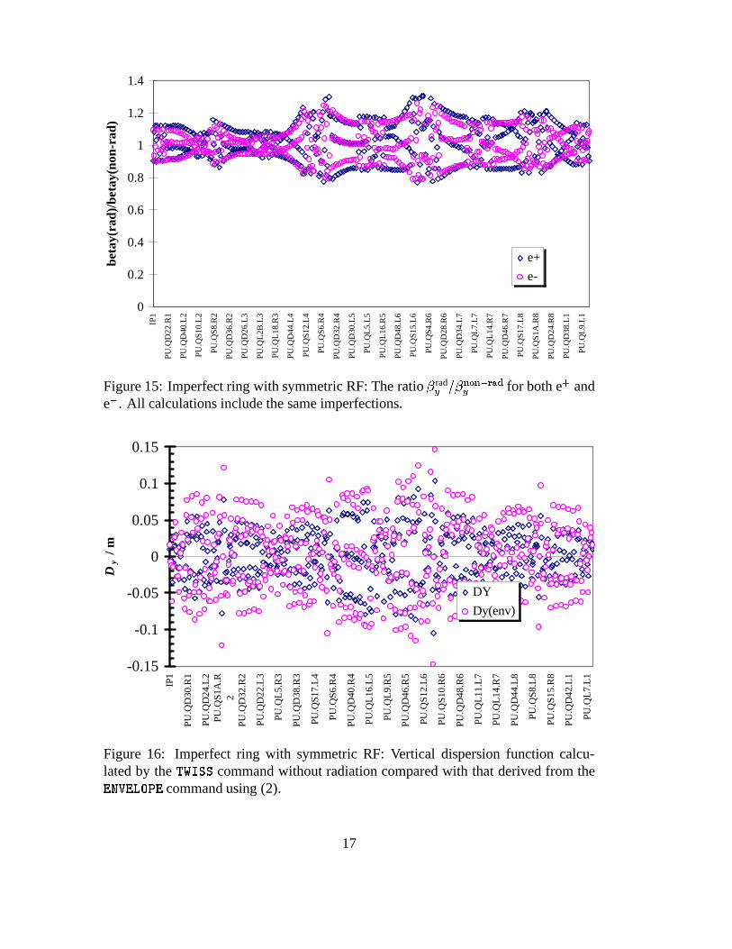
Figure 15 shows that it changes, but does not eliminate, the vertical “�-beating dueto radiation”. The analogues of Figures 4, 5 and 8 (not shown here), are also similar.

Figure 16, the analogue of Figure 9, shows that the difference between the statisticaland TWISS vertical dispersions remains large. This leads to a an over-estimate of thevertical emittance, Figure 18, comparable to the case with asymmetric RF, Figure 11.Figure 12 shows that the beam tilt is again the main source of the problem.

Figure 19 shows that the beam sizes at the IPs remain different, as in Figure 13,despite the symmetric RF. We can conclude that this is due to imperfections. It seems

16

0

0.2

0.4

0.6

0.8

1

1.2

1.4

IP1

PU

.QD

22.R

1

PU

.QD

40.L

2

PU

.QS

10.L

2

PU

.QS

8.R

2

PU

.QD

36.R

2

PU

.QD

26.L

3

PU

.QL2

B.L

3

PU

.QL1

8.R

3

PU

.QD

44.L

4

PU

.QS

12.L

4

PU

.QS

6.R

4

PU

.QD

32.R

4

PU

.QD

30.L

5

PU

.QL5

.L5

PU

.QL1

6.R

5

PU

.QD

48.L

6

PU

.QS

15.L

6

PU

.QS

4.R

6

PU

.QD

28.R

6

PU

.QD

34.L

7

PU

.QL7

.L7

PU

.QL1

4.R

7

PU

.QD

46.R

7

PU

.QS

17.L

8

PU

.QS

1A.R

8

PU

.QD

24.R

8

PU

.QD

38.L

1

PU

.QL9

.L1

beta

y(ra

d)/b

etay

(non

-rad

)

e+

e-

Figure 15: Imperfect ring with symmetric RF: The ratio �rady =�non�rad

y for both e+ ande�. All calculations include the same imperfections.

-0.15

-0.1

-0.05

0

0.05

0.1

0.15

IP1

PU

.QD

30.R

1

PU

.QD

24.L

2P

U.Q

S1A

.R2

PU

.QD

32.R

2

PU

.QD

22.L

3

PU

.QL5

.R3

PU

.QD

38.R

3

PU

.QS

17.L

4

PU

.QS

6.R

4

PU

.QD

40.R

4

PU

.QL1

6.L5

PU

.QL9

.R5

PU

.QD

46.R

5

PU

.QS

12.L

6

PU

.QS

10.R

6

PU

.QD

48.R

6

PU

.QL1

1.L7

PU

.QL1

4.R

7

PU

.QD

44.L

8

PU

.QS

8.L8

PU

.QS

15.R

8

PU

.QD

42.L

1

PU

.QL7

.L1

Dy /

m

DY

Dy(env)

Figure 16: Imperfect ring with symmetric RF: Vertical dispersion function calcu-lated by the TWISS command without radiation compared with that derived from theENVELOPE command using (2).

17

-0.8

-0.6

-0.4

-0.2

0

0.2

0.4

0.6

0.8

IP1

28.R

1

28.L

2

S0.L

2

24.R

2

32.L

3

2B.L

3

24.R

3

32.L

4

S3.L

4

20.R

4

36.L

5

L5.

L5

20.R

5

36.L

6

S5.L

6

17.R

6

40.L

7

L7.

L7

17.R

7

40.L

8

S7.L

8

15.R

8

44.L

1

L9.

L1

R(x,y)+

Figure 17: Imperfect ring with symmetric RF: The beam tilt for positrons computed bythe ENVELOPE command in MAD.

-20.00%

0.00%

20.00%

40.00%

60.00%

80.00%

100.00%

120.00%

140.00%

160.00%

IP1

PU

.QD

30.R

1

PU

.QD

24.L

2P

U.Q

S1A

.R2

PU

.QD

32.R

2

PU

.QD

22.L

3

PU

.QL5

.R3

PU

.QD

38.R

3

PU

.QS

17.L

4

PU

.QS

6.R

4

PU

.QD

40.R

4

PU

.QL1

6.L5

PU

.QL9

.R5

PU

.QD

46.R

5

PU

.QS

12.L

6

PU

.QS

10.R

6

PU

.QD

48.R

6

PU

.QL1

1.L7

PU

.QL1

4.R

7

PU

.QD

44.L

8

PU

.QS

8.L8

PU

.QS

15.R

8

PU

.QD

42.L

1

PU

.QL7

.L1

e+

e-

Figure 18: Imperfect ring with symmetric RF: The fraction by which the vertical emit-tance is over-estimated at each BPM when the true beam size (ENVELOPE) is convertedto an emittance using optical functions calculated by theTWISS command without radi-ation, but with perfect knowledge of the imperfections, according to (1).

18

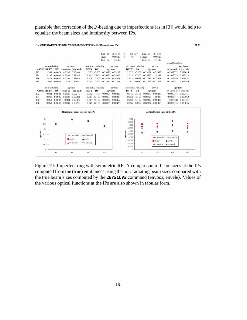
plausible that correction of the �-beating due to imperfections (as in [3]) would help toequalise the beam sizes and luminosity between IPs.

G:\HOME\JOWETT\LEP96\BEUVBEAT\SEED2\OPTICSIN.XLS[Beam sizes at IPs] 21:59 2

Exp / m 2.7E-08 0 82 GeV Exe / m 2.7E-08sigep 0.00129 0 0 0 sigee 0.00129Eyp / m 3E-10 Eye / m 1.7E-10

mixed functionsnon-radiating sigx/mm positrons, radiating envpos electrons, radiating envele sigx / mm

NAME BETX DX + (non-ra- (non-rad) BETX DX sigx/mm BETX DX sigx/mm e+ (mixed) e- (mixed)IP2 2.352 -0.0073 0.2535 0.25403 2.35 -0.007 0.25336 0.25148 2.327 -0.006 0.25201 0.25553 0.2533572 0.252626IP4 3.196 -0.0002 0.2952 0.29587 3.161 7E-04 0.29362 0.29342 3.228 -0.002 0.29672 0.297 0.2936233 0.297373IP6 2.872 0.0031 0.2799 0.28052 2.909 0.003 0.28171 0.28271 2.832 0.0029 0.27793 0.27601 0.2817159 0.278547IP8 1.937 0.0065 0.23 0.23051 2.014 0.004 0.23444 0.23511 1.87 0.0082 0.22608 0.22478 0.2345251 0.226489

non-radiating sigy/mm positrons, radiating envpos electrons, radiating envele sigy/mmNAME BETY DY + (non-ra- (non-rad) BETY DY sigy/mm BETY DY sigy/mm e+ (mixed) e- (mixed)IP2 0.044 -0.0002 0.0036 0.00271 0.042 -1E-04 0.00354 0.00418 0.046 -2E-04 0.00275 0.00389 0.0035371 0.002751IP4 0.048 -0.0005 0.0038 0.00288 0.045 -6E-04 0.00369 0.00425 0.053 -4E-04 0.00296 0.0039 0.0036911 0.002962IP6 0.052 -0.0007 0.004 0.00306 0.049 -9E-04 0.00384 0.00467 0.059 -5E-04 0.00312 0.00406 0.003838 0.003121IP8 0.051 0.0001 0.0039 0.00291 0.048 -8E-05 0.00379 0.00429 0.056 0.0002 0.00304 0.00355 0.0037915 0.003035

Horizontal beam sizes at the IPs

0

0.05

0.1

0.15

0.2

0.25

0.3

IP2 IP4 IP6 IP8

sigx

/ m

m

e+ (non-rad) e- (non-rad)

envpos envele

e+ (mixed) e- (mixed)

Vertical beam sizes at the IPs

0

0.0005

0.001

0.0015

0.002

0.0025

0.003

0.0035

0.004

0.0045

0.005

IP2 IP4 IP6 IP8

sigx

/ m

m

e+ (non-rad) e- (non-rad)

envpos envele

e+ (mixed) e- (mixed)

G:\HOME\JOWETT\LEP96\BEUVBEAT\SEED2\OPTICSIN.XLS[Beam sizes at IPs] 21:59 2

Figure 19: Imperfect ring with symmetric RF: A comparison of beam sizes at the IPscomputed from the (true) emittances using the non-radiating beam sizes compared withthe true beam sizes computed by the ENVELOPE command (envpos, envele). Values ofthe various optical functions at the IPs are also shown in tabular form.

19

3.3 Perfect machine with symmetric RF

As a further check on the origin of the effects, this section considers the case of a perfectmachine with the same symmetric RF configuration as in Section 3.2. Of course thereis now no vertical dispersion or excitation of the vertical emittance so fewer quantitiescan be compared.

Nevertheless, Figure 20 shows that the horizontal beam sizes are virtually identicalfor the two beams9

0

0.5

1

1.5

2

2.5

3

IP1

PU

.QD

22.R

1

PU

.QD

40.L

2

PU

.QS

10.L

2

PU

.QS

8.R

2

PU

.QD

36.R

2

PU

.QD

26.L

3

PU

.QL2

B.L

3

PU

.QL1

8.R

3

PU

.QD

44.L

4

PU

.QS

12.L

4

PU

.QS

6.R

4

PU

.QD

32.R

4

PU

.QD

30.L

5

PU

.QL5

.L5

PU

.QL1

6.R

5

PU

.QD

48.L

6

PU

.QS

15.L

6

PU

.QS

4.R

6

PU

.QD

28.R

6

PU

.QD

34.L

7

PU

.QL7

.L7

PU

.QL1

4.R

7

PU

.QD

46.R

7

PU

.QS

17.L

8

PU

.QS

1A.R

8

PU

.QD

24.R

8

PU

.QD

38.L

1

PU

.QL9

.L1

sigx

/ mm

envpos

envele

Figure 20: Perfect ring: The true horizontal beam size (ENVELOPE command) at all theBPMs and IPs around the ring for both e+ and e�.

The “�-beating due to radiation”, Figure 21, is now more symmetric but has essen-tially the same magnitude.

The horizontal dispersion computed from the statistical definition, (2) is in goodagreement with that computed by the TWISS command without radiation and RF (Fig-ure 22). However the analogue of Figure 10 (not shown) still shows an over-estimateof the horizontal emittance of about 10 %.

The analogue of Figure 13, Figure 23, shows that the horizontal beam sizes are nowall equal and predicted well by any method.

9I believe, but have not checked in detail, that the small antisymmetries around the IPs are due to thesmall differences in layout and optics between the interaction regions.

20

0

0.2

0.4

0.6

0.8

1

1.2

IP1

PU

.QD

22.R

1

PU

.QD

40.L

2

PU

.QS

10.L

2

PU

.QS

8.R

2

PU

.QD

36.R

2

PU

.QD

26.L

3

PU

.QL2

B.L

3

PU

.QL1

8.R

3

PU

.QD

44.L

4

PU

.QS

12.L

4

PU

.QS

6.R

4

PU

.QD

32.R

4

PU

.QD

30.L

5

PU

.QL5

.L5

PU

.QL1

6.R

5

PU

.QD

48.L

6

PU

.QS

15.L

6

PU

.QS

4.R

6

PU

.QD

28.R

6

PU

.QD

34.L

7

PU

.QL7

.L7

PU

.QL1

4.R

7

PU

.QD

46.R

7

PU

.QS

17.L

8

PU

.QS

1A.R

8

PU

.QD

24.R

8

PU

.QD

38.L

1

PU

.QL9

.L1

beta

y(ra

d)/b

etay

(non

-rad

)

e+

e-

Figure 21: Perfect ring: The ratio �rady =�non�rad

y for both e+ and e�. All calculationsinclude the same imperfections.

-0.1

0.1

0.3

0.5

0.7

0.9

1.1

IP1

PU

.QD

28.R

1

PU

.QD

28.L

2

PU

.QS

0.L2

PU

.QD

24.R

2

PU

.QD

32.L

3

PU

.QL2

B.L

3

PU

.QD

24.R

3

PU

.QD

32.L

4

PU

.QS

3.L4

PU

.QD

20.R

4

PU

.QD

36.L

5

PU

.QL5

.L5

PU

.QD

20.R

5

PU

.QD

36.L

6

PU

.QS

5.L6

PU

.QS

17.R

6

PU

.QD

40.L

7

PU

.QL7

.L7

PU

.QL1

7.R

7

PU

.QD

40.L

8

PU

.QS

7.L8

PU

.QS

15.R

8

PU

.QD

44.L

1

PU

.QL9

.L1

Dx /

m

DX

Dx(env)

Figure 22: Perfect ring: Horizontal dispersion function calculated by the TWISS com-mand without radiation compared with that derived from the ENVELOPE command us-ing (2).

21

G:\HOME\JOWETT\LEP96\BEUVBEAT\PERFECT\OPTICSIN.XLS[Beam sizes at IPs] 23:50 2

Exp / m 2.6E-08 0 82 GeV Exe / m 2.6E-08sigep 0.00129 0 0 0 sigee 0.00129Eyp / m 0 Eye / m 0

mixed functionsnon-radiating sigx/mm positrons, radiating envpos electrons, radiating envele sigx / mm

NAME BETX DX + (non-ra- (non-rad) BETX DX sigx/mm BETX DX sigx/mm e+ (mixed) e- (mixed)IP2 2.5 -2E-08 0.2526 0.25258 2.495 8E-05 0.25232 0.25232 2.498 0.0006 0.25246 0.25248 0.25232 0.252475IP4 2.5 2E-08 0.2526 0.25258 2.501 2E-04 0.25262 0.25262 2.5 -8E-04 0.25258 0.2526 0.2526237 0.252596IP6 2.5 -2E-08 0.2526 0.25258 2.497 -6E-04 0.25239 0.25239 2.492 0.0005 0.25217 0.25219 0.2523847 0.252188IP8 2.5 1E-08 0.2526 0.25258 2.508 4E-04 0.25294 0.25294 2.494 -1E-04 0.25224 0.25225 0.2529391 0.252253

non-radiating sigy/mm positrons, radiating envpos electrons, radiating envele sigy/mmNAME BETY DY + (non-ra- (non-rad) BETY DY sigy/mm BETY DY sigy/mm e+ (mixed) e- (mixed)IP2 0.05 0 0 0 0.051 -2E-27 0 1E-16 0.051 4E-28 0 1.9E-16 0 0IP4 0.05 0 0 0 0.051 -6E-28 0 1E-16 0.051 -4E-28 0 1.9E-16 0 0IP6 0.05 0 0 0 0.051 -7E-28 0 1E-16 0.051 -7E-28 0 2E-16 0 0IP8 0.05 0 0 0 0.051 3E-28 0 1E-16 0.051 -7E-28 0 2E-16 0 0

Horizontal beam sizes at the IPs

0

0.05

0.1

0.15

0.2

0.25

0.3

IP2 IP4 IP6 IP8

sigx

/ m

m

e+ (non-rad) e- (non-rad)

envpos envele

e+ (mixed) e- (mixed)

Figure 23: Perfect ring: A comparison of beam sizes at the IPs computed from the (true)emittances using the non-radiating beam sizes compared with the true beam sizes com-puted by the ENVELOPE command (envpos, envele). Values of the various optical func-tions at the IPs are also shown in tabular form.

22

4 Conclusions

The simulations above illustrate the following points:

� The vertical emittances of positrons and electrons can easily be substantially dif-ferent at high energy. The differences are not due to the asymmetry of the RFvoltage distribution but rather to the distribution of the imperfections generatingthe vertical emittance.

� Similar remarks hold for the optical functions.

� Using optical functions—the dispersion in particular—calculated without the in-clusion of radiation can lead to substantial errors in the conversion of a measuredvertical beam size into a value for the vertical emittance. The same procedure inthe horizontal plane gives numerically acceptable results.

� With small values of the emittance ratio, the tilt of the beam ellipse in configu-ration space can be large enough to confound the attempt to convert a measuredvertical beam size directly into an emittance.

� It may be possible to provide a better estimate of the vertical emittance using thevalue of the correlation function hxyi together with the mean-square beam sizeshx2i and hy2i. The formula

�y =hx2i hy2i � hxyi2

�y hx2i: (4)

neglects terms describing the coupling of the second mode back into the firstand certainly applies only when the dispersion at the BEUV monitors can be ne-glected. The quantities appearing on the right-hand side are all accessible to mea-surement. The function�y should be computed with radiation included (althoughthis is still an approximation). I have tried this with the numerical data describedabove but, unfortunately, it did not work much better as an estimator of �y .

It may be objected that the vertical emittances in the imperfect machine consid-ered above were too small, exaggerating the errors and differences between beams.To check this, I repeated the calculations with another seed for the random imperfec-tions and larger amplitudes of the random tilts. The resulting emittances were larger,�+y = 5:2 nm and ��y = 1:7 nm, but the other results confirmed most of the above con-clusions except that the overestimate of vertical emittance from beam size was less,typically 20 %. Application of (4) also worked a little better.

As a final conclusion, I consider that it is worth implementing (4) as an improvedmethod for estimating the vertical emittance in operation. However it cannot be ex-pected to work well for small �y. If reliable vertical dispersion values are availablefrom measurements they might also be incorporated (together with the computed en-ergy spread) as a correction to this formula.

23

References

[1] P. Castro et al, “Cross-calibration of emittance measuring instruments in LEP”,CERN SL–MD Note 202 (1996).

[2] M. Lamont, SL Performance Committee meeting of 17 April 1996.

[3] E. Keil, “Off-line simulation of beta-beating correction”, CERN SL Note 96–25(AP) (1996).

[4] H. Grote, F.C. Iselin, “The MAD program (Methodical Accelerator Design) : Ver-sion 8.16 ; User’s Reference Manual”, CERN SL 90–13 (AP) rev. 4 (1995). Themanual for the version of MAD used in this note is presently available on theWorld-Wide Web at http://hpariel.cern.ch/fci/mad/mad.html

[5] A.W. Chao, “Evaluation of beam distribution parameters in an electron storagering”, J. Appl. Phys. 50(2), 1979

[6] J.M. Jowett, “Problems expected from RF asymmetries”, in J. Poole (Ed.), Pro-ceedings of the Sixth Workshop on LEP Performance, Chamonix, January 1996,CERN SL/96-05 (DI) (1996).

[7] J.M. Jowett, “RF Voltage Distribution in LEP with MAD”, CERN SL Note 96–29(AP) (1996).

24