
Beam-beam e ects - The CERN Accelerator...
69
Beam-beam effects (an introduction) Werner Herr CERN, AB Department (/afs/ictp/home/w/wfherr/public/CAS/doc/beambeam.pdf ) (http://cern.ch/lhc-beam-beam/talks/Trieste beambeam.pdf ) Werner Herr, beam-beam effects, CAS 2005, Trieste
Transcript of Beam-beam e ects - The CERN Accelerator...
Beam-beam effects
(an introduction)
Werner HerrCERN, AB Department
(/afs/ictp/home/w/wfherr/public/CAS/doc/beambeam.pdf)
(http://cern.ch/lhc-beam-beam/talks/Trieste beambeam.pdf)
Werner Herr, beam-beam effects, CAS 2005, Trieste

BEAMS: moving charges
Beam is a collection of charges
Represent electromagnetic potential for other
charges
Forces on itself (space charge) and opposing
beam (beam-beam effects)
Main limit for present and future colliders
Important for high density beams, i.e. high
intensity and/or small beams:
for high luminosity !
Beam-beam effects
Remember:
=⇒ L =N1N2fB
4πσxσy
=N1N2fB
4π · σxσy
Overview: which effects are important for
present and future machines (LEP, PEP,
Tevatron, RHIC, LHC, ...)
Qualitative and physical picture of the effects
Mathematical derivations in:
Proceedings, Zeuthen 2003
Beam-beam effects
A beam acts on particles like an
electromagnetic lens, but:
Does not represent simple form, i.e. well
defined multipoles
Very non-linear form of the forces, depending
on distribution
Can change distribution as result of
interaction (time dependent forces ..)
Results in many different effects and problems

Fields and Forces (I)
Start with a point charge q and integrate over
the particle distribution ρ(~x).
In rest frame only electrostatic field: ~E ′,
but ~B′ ≡ 0
Transform into moving frame and calculate
Lorentz force
E‖ = E ′‖, E⊥ = γ · E ′
⊥ with : ~B = ~β × ~E/c
~F = q( ~E + ~β × ~B)

Fields and Forces (II)
Derive potential U(x, y, z) from Poisson
equation:
∆U(x, y, z) = − 1
ε0
ρ(x, y, z)
The fields become:
~E = −∇U(x, y, z)
Example Gaussian distribution:
ρ(x, y, z) =Ne
σxσyσz
√2π
3 exp
(
− x2
2σ2x
− y2
2σ2y
− z2
2σ2z
)
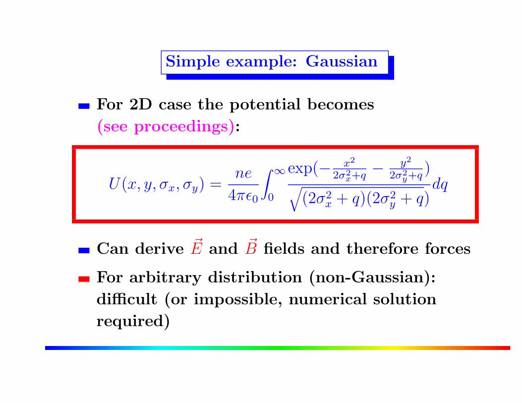
Simple example: Gaussian
For 2D case the potential becomes
(see proceedings):
U(x, y, σx, σy) =ne
4πε0
∫ ∞
0
exp(− x2
2σ2x+q
− y2
2σ2y+q
)√
(2σ2x + q)(2σ2
y + q)dq
Can derive ~E and ~B fields and therefore forces
For arbitrary distribution (non-Gaussian):
difficult (or impossible, numerical solution
required)

Simple example: Gaussian
Round beams: σx = σy = σ
Only components Er and BΦ are non-zero
Force has only radial component, i.e. depends
only on distance r from bunch centre
(where: r2 = x2 + y2) (see proceedings)
Fr(r) = −ne2(1 + β2)
2πε0 · r
[
1 − exp(− r2
2σ2)
]

Beam-beam kick:
Kick (∆r′): angle by which the particle is
deflected during the passage
Derived from force by integration over the
collision (assume: m1=m2 and β1=β2):
Fr(r, s, t) = − Ne2(1 + β2)√
(2π)3ε0rσs
[
1 − exp(− r2
2σ2)
]
·[
exp(− (s + vt)2
2σ2s
)
]
with Newton′s law : ∆r′ =1
mcβγ
∫ ∞
∞
Fr(r, s, t)dt
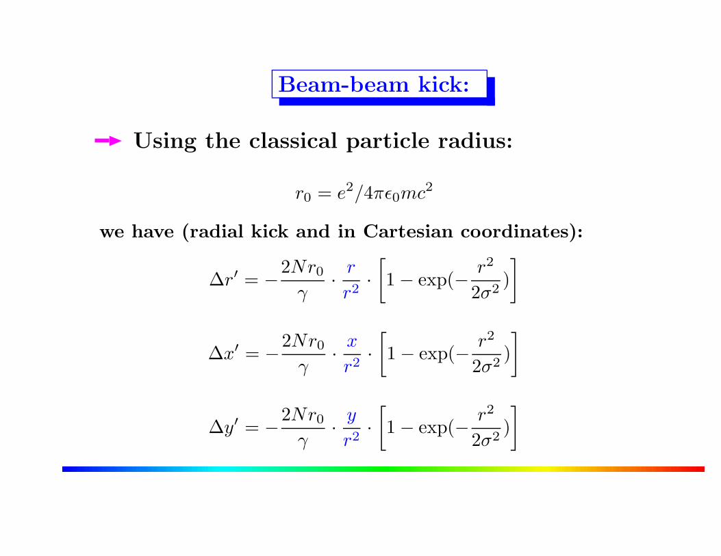
Beam-beam kick:
Using the classical particle radius:
r0 = e2/4πε0mc2
we have (radial kick and in Cartesian coordinates):
∆r′ = −2Nr0
γ· r
r2·[
1 − exp(− r2
2σ2)
]
∆x′ = −2Nr0
γ· x
r2·[
1 − exp(− r2
2σ2)
]
∆y′ = −2Nr0
γ· y
r2·[
1 − exp(− r2
2σ2)
]

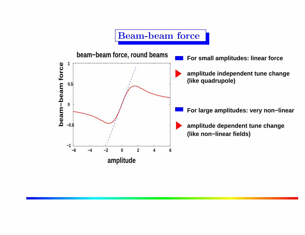
Beam-beam force
6 4 2 0−2−4−6−1
−0.5
0
0.5
1b
ea
m−
be
am
fo
rce
beam−beam force, round beams
amplitude
� � � �
� � � �
� � � �
� � � �
� � � �
� � � �
� � � �
� � � �
� � � �
� � � �
� � � �
� � � �
� � �
� � �
� � �
� � �
� � �
� � �
� � �
� � �
� � �
� � �
� � �
amplitudeForce varies strongly with
Exponential function:
Contains many high order multipoles
Beam-beam force
6 4 2 0−2−4−6−1
−0.5
0
0.5
1b
ea
m−
be
am
fo
rce
beam−beam force, round beams
amplitude
� � � �� � � �� � � �
� � � �� � � �� � � �� �� �� �� �� �� �� �� �� �� �� �� �
� � � �� � � �� � � �
� � � �� � � �� � � �
� � �� � �� � �� � �� � �� � �� � �� � �� � �� � �
For large amplitudes: very non−linear
For small amplitudes: linear force
amplitude independent tune change
amplitude dependent tune change
(like quadrupole)
(like non−linear fields)

Can we measure the beam-beam strength ?
Try the slope of force at zero amplitude → proportional
to (linear) tune shift ∆ Qbb from beam-beam interaction
This defines: beam-beam parameter ξ
For head-on interactions we get:
ξx,y =
N ·ro·βx,y
2πγσx,y(σx+σy)
BUT: does not describe non-linear part of beam-beam
force (so far: only an additional quadrupole !)

Tune measurement: linear optics
1.2
0.8
0.4
0
Tune distribution for linear optics
0.2800.276 0.278
Qx
� � �� � �� � �� � �� � �� � �
� � �� � �� � �� � �� � �� � �
� �� �� �� �� �� �� �� �� �� �� �� �
Only one frequency (tune) visible
all particles have same tune
Linear force:
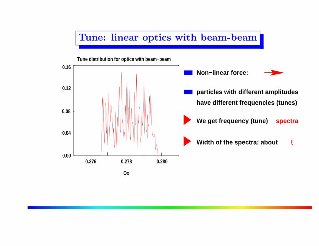
Tune: linear optics with beam-beam
0.16
0.12
0.08
0.04
0.00
Qx
Tune distribution for optics with beam−beam
0.2800.2780.276
� � �� � �� � �� � �� � �� � �
� �� �� �� �� �� �� �� �� �� �� �� �
� � �� � �� � �� � �� � �� � �� � �� � �
� �� �� �� �� �� �� �� �� �� �
Non−linear force:
particles with different amplitudes
have different frequencies (tunes)
We get frequency (tune) spectra
Width of the spectra: about ξ
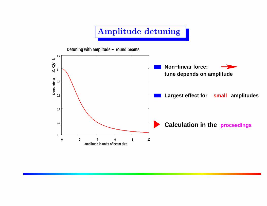
Amplitude detuning
Q/
∆ξ
Detuning with amplitude − round beams
amplitude in units of beam size
De
tun
ing
0.8
0.6
0.4
0.2
0
1
1.2
0 2 4 106 8
amplitudesLargest effect for small� � �� � �� � �� � �� � �� � �
� � �� � �� � �� � �� � �� � �
� �� �� �� �� �� �� �� �� �� �� �
Non−linear force:tune depends on amplitude
Calculation in the proceedings
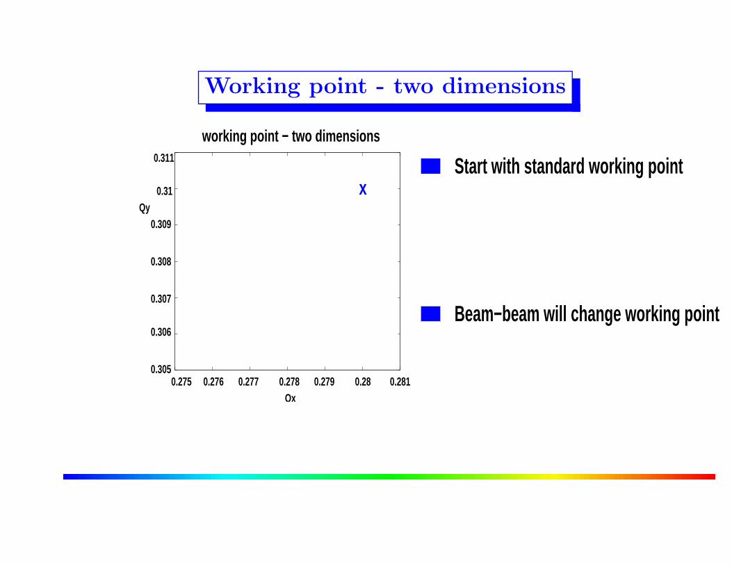
Working point - two dimensions
0.277 0.278 0.279 0.28 0.281Qx
0.2760.2750.305
0.306
0.307
0.308
0.309Qy
0.31
0.311
x
working point − two dimensions
� � � �
� � � �
� � � �
� � �
� � �
� � �
� � � �
� � � �
� � � �
� � �
� � �
� � �
Start with standard working point
Beam−beam will change working point

Linear tune shift - two dimensions
0.277 0.278 0.279 0.28 0.281Qx
0.2760.2750.305
0.306
0.307
0.308
0.309Qy
0.31
0.311
x
Tune shift for head−on collision
x� � � �
� � � �
� � � �
� � �
� � �
� � �
� � � �
� � � �
� � � �
� � �
� � �
� � �
Start with standard working point
Tunes shifted in both planes
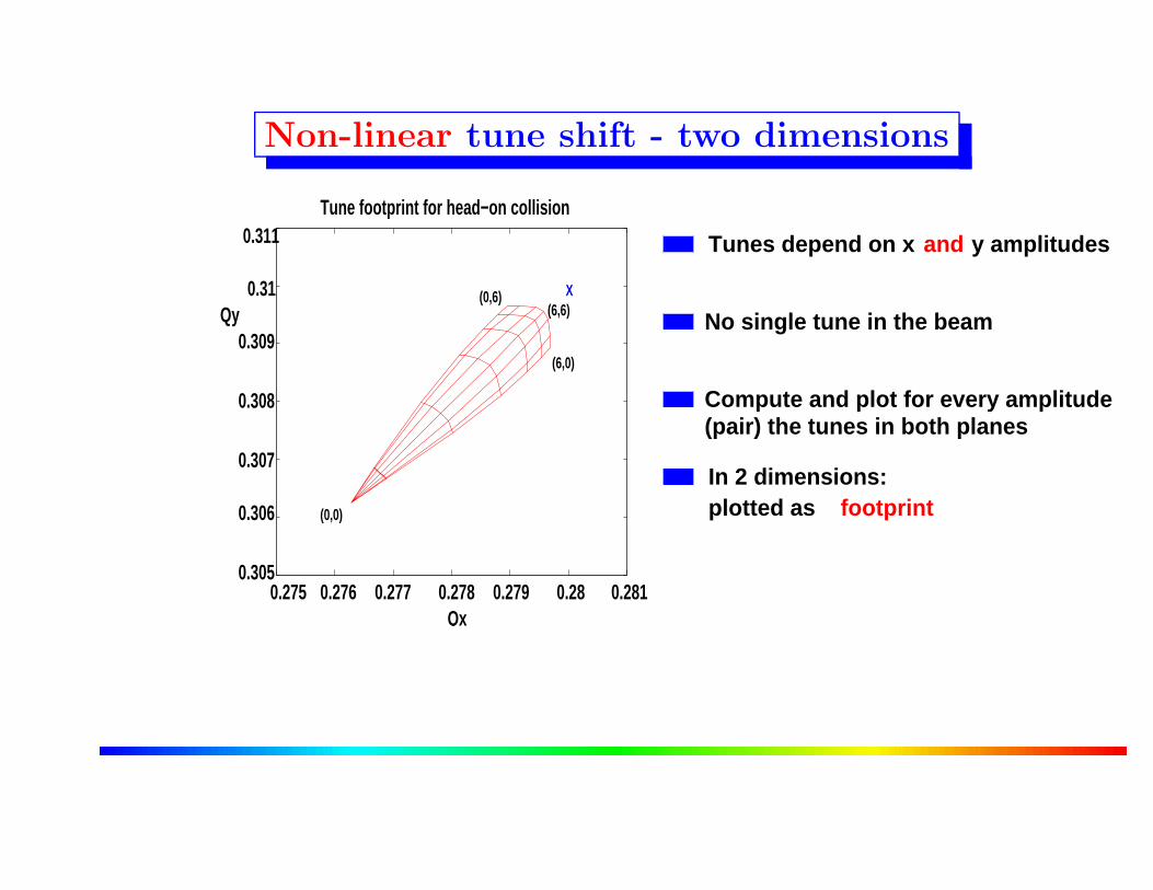
Non-linear tune shift - two dimensions
0.277 0.278 0.279 0.28 0.281Qx
0.2760.2750.305
0.306
0.307
0.308
0.309Qy
0.31
0.311Tune footprint for head−on collision
(0,0)
X(6,6)
(6,0)
(0,6)
Tunes depend on x y amplitudesand
� � � �
� � � �
� � � �
� � �
� � �
� � �
� � � �
� � � �
� � � �
� � � �
� � �
� � �
� � �
� � �
� � � �
� � � �
� � � �
� � �
� � �
� � �
� � � �
� � � �
� � � �
� � � �
� � �
� � �
� � �
� � �
In 2 dimensions:plotted as footprint
No single tune in the beam
Compute and plot for every amplitude(pair) the tunes in both planes
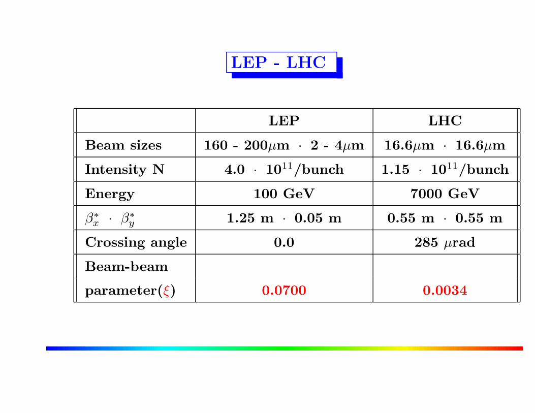
LEP - LHC
LEP LHC
Beam sizes 160 - 200µm · 2 - 4µm 16.6µm · 16.6µm
Intensity N 4.0 · 1011/bunch 1.15 · 1011/bunch
Energy 100 GeV 7000 GeV
β∗x · β∗
y 1.25 m · 0.05 m 0.55 m · 0.55 m
Crossing angle 0.0 285 µrad
Beam-beam
parameter(ξ) 0.0700 0.0034

Weak-strong and strong-strong
Both beams are very strong (strong-strong):
→ Both beam are affected and change due to
beam-beam interaction
→ Examples: LHC, LEP, RHIC, ...
One beam much stronger (weak-strong):
→ Only the weak beam is affected and changed
due to beam-beam interaction
→ Examples: SPS collider, Tevatron, ...

Incoherent effects
(single particle effects)
Single particle dynamics: treat as a particle
through a static electromagnetic lens
Basically non-linear dynamics
All single particle effects observed:
→ Unstable and/or irregular motion
→ beam blow up or bad lifetime
Observations hadrons
Non-linear motion can become chaotic
→ reduction of ”dynamic aperture”
→ particle loss and bad lifetime
Strong effects in the presence of noise or ripple
Very bad: unequal beam sizes (studied at SPS,
HERA)
Evaluation is done by simulation
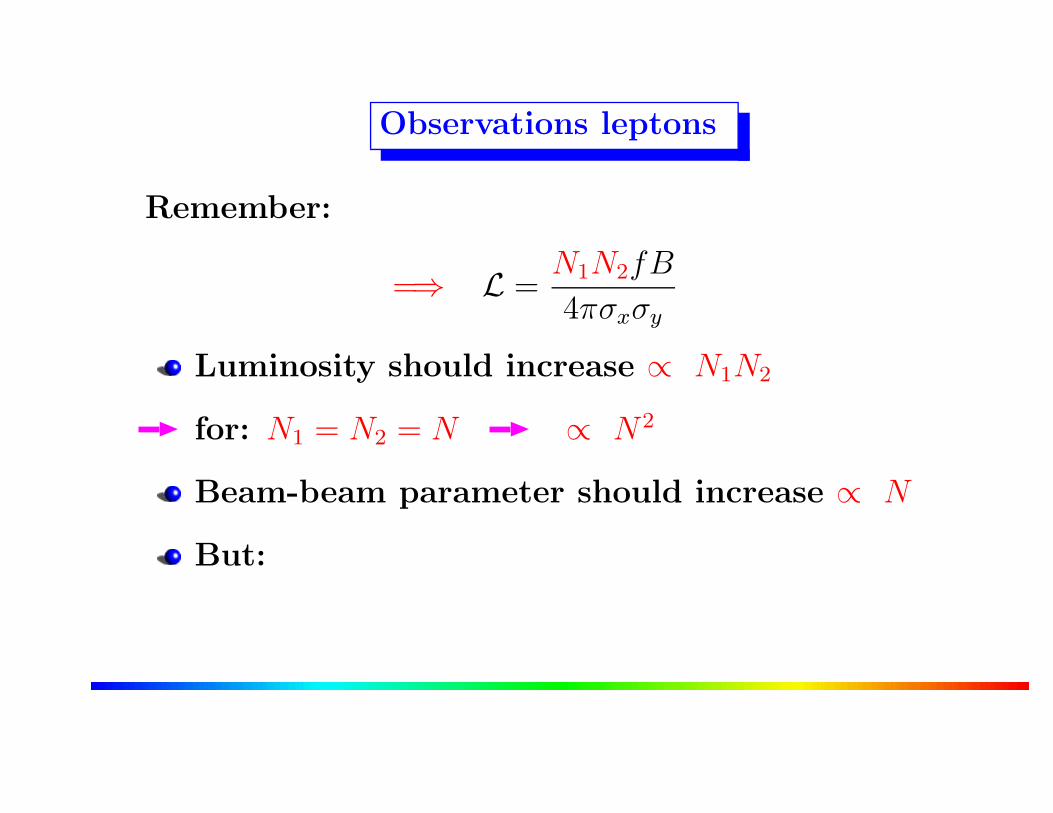
Observations leptons
Remember:
=⇒ L =N1N2fB
4πσxσy
Luminosity should increase ∝ N1N2
for: N1 = N2 = N ∝ N 2
Beam-beam parameter should increase ∝ N
But:
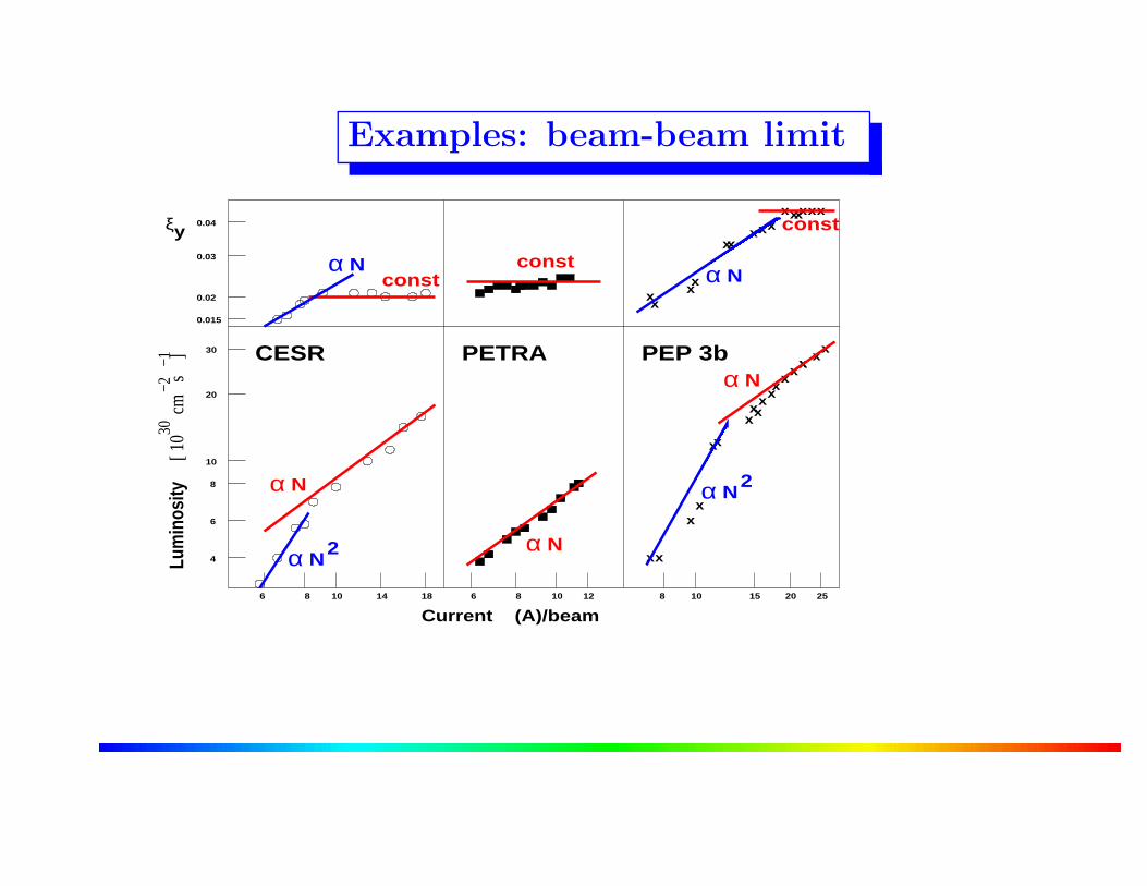
Examples: beam-beam limit
0.04
0.02
0.03
0.015
30
20
10
8
6
4
10 8 15 252010128618141086
xx
xx
xx
xxxxx
xxxx
x
xx
xxxx
xxxxx
xxxxxx
PEP 3bPETRACESR
Current (A)/beam
Lum
inos
ity[ 1
0
cm
s
]30
−2
−1
ξy
� � � � � � � � � � �� � � � � � � � � � �
� � � � � � � � � �� � � � � � � � �
� � � � � � � � � � � � �� � � � � � � � � � � � �� � � � � � � � � � � � �� � � � � � � � � � � � �� � � � � � � � � � � � �� � � � � � � � � � � � �� � � � � � � � � � � � �� � � � � � � � � � � � �� � � � � � � � � � � � �� � � � � � � � � � � � �� � � � � � � � � � � � �� � � � � � � � � � � � �� � � � � � � � � � � � �� � � � � � � � � � � � �� � � � � � � � � � � � �� � � � � � � � � � � � �� � � � � � � � � � � � �� � � � � � � � � � � � �� � � � � � � � � � � � �� � � � � � � � � � � � �� � � � � � � � � � � � �� � � � � � � � � � � � �� � � � � � � � � � � � �
� � � � � � � � � � � �� � � � � � � � � � � �� � � � � � � � � � � �� � � � � � � � � � � �� � � � � � � � � � � �� � � � � � � � � � � �� � � � � � � � � � � �� � � � � � � � � � � �� � � � � � � � � � � �� � � � � � � � � � � �� � � � � � � � � � � �� � � � � � � � � � � �� � � � � � � � � � � �� � � � � � � � � � � �� � � � � � � � � � � �� � � � � � � � � � � �� � � � � � � � � � � �� � � � � � � � � � � �� � � � � � � � � � � �� � � � � � � � � � � �� � � � � � � � � � � �� � � � � � � � � � � �� � � � � � � � � � � �
� � � � � � � � � � �� � � � � � � � � � �� � � � � � � � � � �� � � � � � � � � � �� � � � � � � � � � �� � � � � � � � � � �� � � � � � � � � � �� � � � � � � � � � �� � � � � � � � � � �� � � � � � � � � � �� � � � � � � � � � �� � � � � � � � � � �� � � � � � � � � � �� � � � � � � � � � �� � � � � � � � � � �� � � � � � � � � � �� � � � � � � � � � �
� � � � � � � � � � �� � � � � � � � � � �� � � � � � � � � � �� � � � � � � � � � �� � � � � � � � � � �� � � � � � � � � � �� � � � � � � � � � �� � � � � � � � � � �� � � � � � � � � � �� � � � � � � � � � �� � � � � � � � � � �� � � � � � � � � � �� � � � � � � � � � �� � � � � � � � � � �� � � � � � � � � � �� � � � � � � � � � �
� � � � � � � � � �� � � � � � � � � �� � � � � � � � � �� � � � � � � � � �� � � � � � � � � �� � � � � � � � � �� � � � � � � � � �� � � � � � � � � �� � � � � � � � � �� � � � � � � � � �� � � � � � � � � �� � � � � � � � � �� � � � � � � � � �� � � � � � � � � �� � � � � � � � � �
� � � � � � �� � � � � � �� � � � � � �� � � � � � �� � � � � � �� � � � � � �� � � � � � �� � � � � � �� � � � � � �
� � � � �� � � � �� � � � �� � � � �� � � � �� � � � �� � � � �� � � � �� � � � �� � � � �� � � � �� � � � �� � � � �� � � � �
� � � � � � � � � � � �� � � � � � � � � � � �� � � � � � � � � � � �� � � � � � � � � � � �� � � � � � � � � � � �� � � � � � � � � � � �� � � � � � � � � � � �� � � � � � � � � � � �� � � � � � � � � � � �� � � � � � � � � � � �� � � � � � � � � � � �� � � � � � � � � � � �� � � � � � � � � � � �� � � � � � � � � � � �� � � � � � � � � � � �� � � � � � � � � � � �� � � � � � � � � � � �
� � � � � � � � � � �� � � � � � � � � � �� � � � � � � � � � �� � � � � � � � � � �� � � � � � � � � � �� � � � � � � � � � �� � � � � � � � � � �� � � � � � � � � � �� � � � � � � � � � �� � � � � � � � � � �� � � � � � � � � � �� � � � � � � � � � �� � � � � � � � � � �� � � � � � � � � � �� � � � � � � � � � �� � � � � � � � � � �
� � � � � � �� � � � � � �� � � � � � �� � � � � � �� � � � � � �� � � � � � �� � � � � � �� � � � � � �� � � � � � �� � � � � � �� � � � � � �� � � � � � �� � � � � � �� � � � � � �� � � � � � �� � � � � � �� � � � � � �� � � � � � �� � � � � � �� � � � � � �� � � � � � �� � � � � � �� � � � � � �� � � � � � �� � � � � � �
� � � � � �� � � � � �� � � � � �� � � � � �� � � � � �� � � � � �� � � � � �� � � � � �� � � � � �� � � � � �� � � � � �� � � � � �� � � � � �� � � � � �� � � � � �� � � � � �� � � � � �� � � � � �� � � � � �� � � � � �� � � � � �� � � � � �� � � � � �� � � � � �� � � � � �
N2
NN
N2
N
N
N
α
α
α
α
α
α αconstconst
const
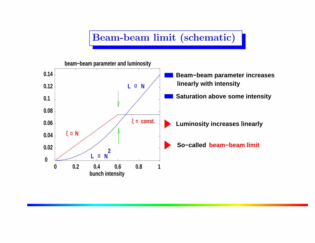
Beam-beam limit (schematic)
bunch intensity
beam−beam parameter and luminosity
0.14
0.12
0.1
0.06
0.08
0.04
0.02
00 0.2 0.4 0.6 0.8 1
ξ = const.
Nξ
L N
L N2
α
α
α
beam−beam limitSo−called� � �� � �� � �� � �� � �� �� �� �� �� �
� � � �� � � �� � � �� � �� � �� � �
� � � �� � � �� � � �� � � �� � �� � �� � �� � �
� � �� � �� � �� � �� � �� � �� �� �� �� �� �� �
Beam−beam parameter increaseslinearly with intensity
Saturation above some intensity
Luminosity increases linearly

What is happening ?
we have ξy =Nr0βy
2πγσy(σx + σy)
(σx � σy)≈ r0βy
2πγ(σx)· N
σy
and L =N2fB
4πσxσy
=NfB
4πσx
· N
σy
Above beam-beam limit: σy increases when N increases
to keep ξ constant equilibrium emittance !
Therefore: L ∝ N and ξ ≈ constant
ξlimit is NOT a universal constant !
Difficult to predict
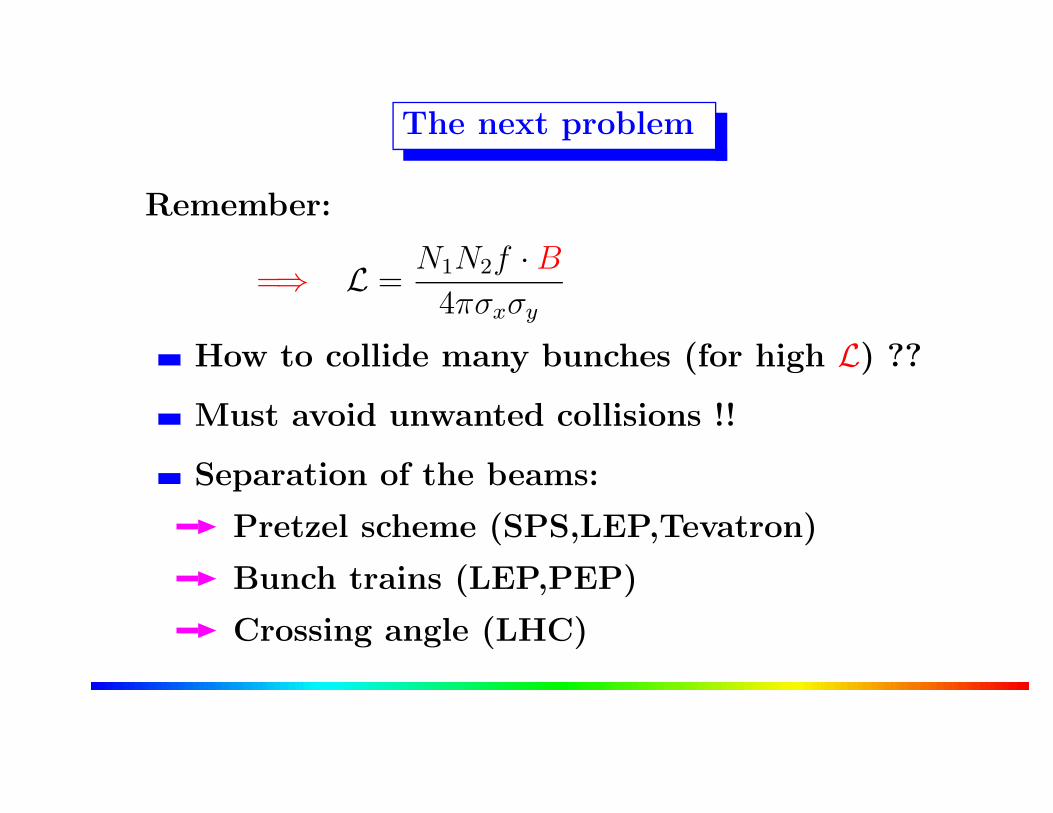
The next problem
Remember:
=⇒ L =N1N2f · B
4πσxσy
How to collide many bunches (for high L) ??
Must avoid unwanted collisions !!
Separation of the beams:
Pretzel scheme (SPS,LEP,Tevatron)
Bunch trains (LEP,PEP)
Crossing angle (LHC)

Separation: SPS
⇒ Few equidistant bunches
(6 against 6)
Beams travel in same beam pipe
(12 collision points !)
Two experimental areas
Need global separation
Horizontal pretzel around most of the
circumference

Separation: SPS
IP 6
IP 1
IP 2
IP 3
IP 4 - UA2
IP 5 - UA 1
antiproton orbit for operationwith 6 * 6 bunches
electrostatic separators
electrostatic separators
proton orbit for operation with 6 * 6 bunches
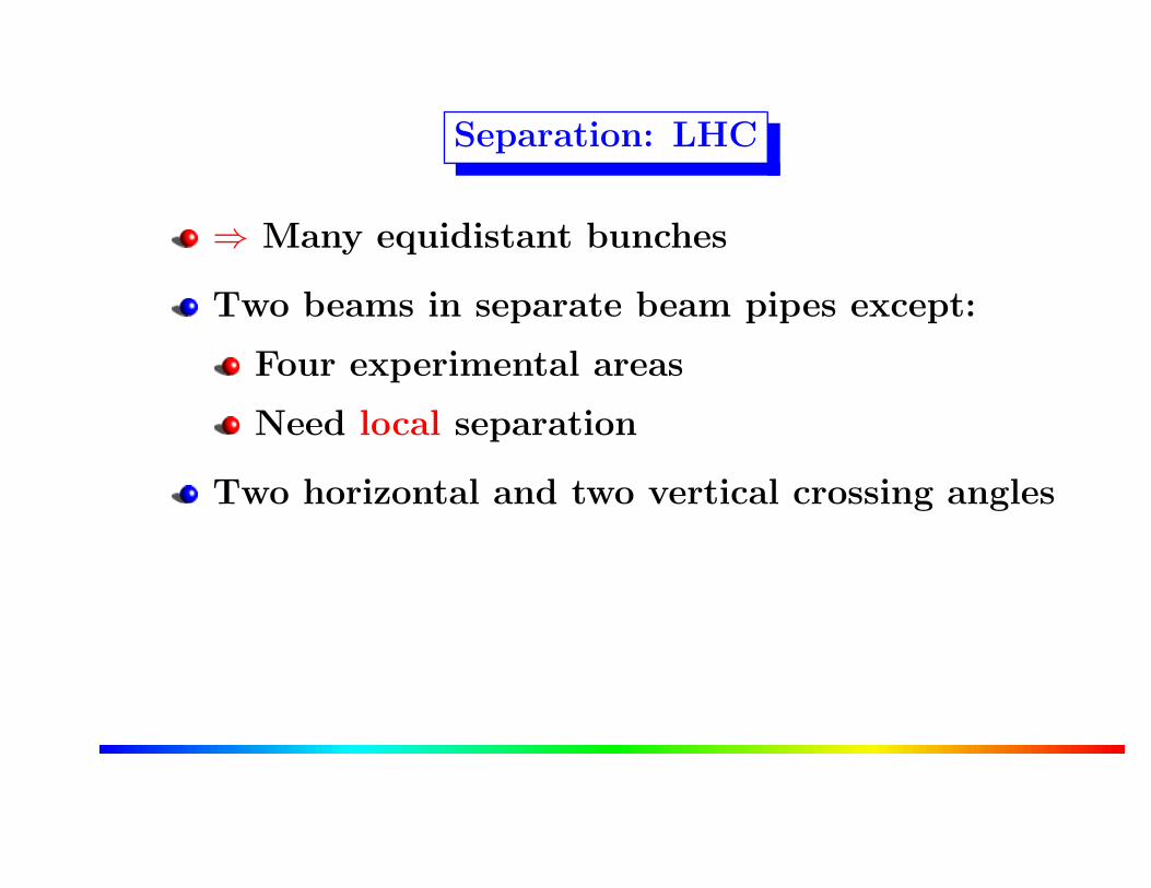
Separation: LHC
⇒ Many equidistant bunches
Two beams in separate beam pipes except:
Four experimental areas
Need local separation
Two horizontal and two vertical crossing angles

Layout of LHC
IP1
beam2beam1
IP3
IP8
IP5
IP6
IP7
IP4
IP2

Crossing angles (example LHC)
� � � � � �
� � � � � �
� � � � � �
� � � � � �
� � � � � �
� � � � � �
� � � � � �
� � � � � �
� � � � � �
� � � � � �
Head-on
� � � � � �
� � � � � �
� � � � � �
� � � � � �
� � � � � �
� � � � � �
� � � � � �
� � � � � �
Long-range
Still some parasitic interactions
Particles experience distant (weak) forces
We get so-called long range interactions
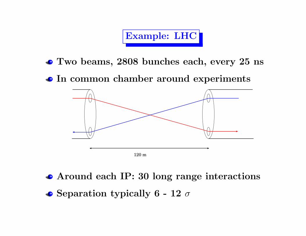
Example: LHC
Two beams, 2808 bunches each, every 25 ns
In common chamber around experiments
120 m
Around each IP: 30 long range interactions
Separation typically 6 - 12 σ
What is special about them ?
Break symmetry between planes, also odd
resonances
Mostly affect particles at large amplitudes
Tune shift has opposite sign in plane of
separation
Cause effects on closed orbit
PACMAN effects

Opposite tuneshift ???
BEAM−BEAM FORCE, ROUND BEAMS
−0.8
−0.6
−0.4
−0.2
0
0.2
0.4
0.6
0.8
−6 −4 −2 0 2 4 6
head on long range
� �� �� �� �� �� �� �� �
� �� �� �� �� �� �� �� �
� � �� � �� � �� � �� �� �� �� �
Used for partial compensation
Opposite sign for focusing
sign for large separation
Local slope of force has opposite
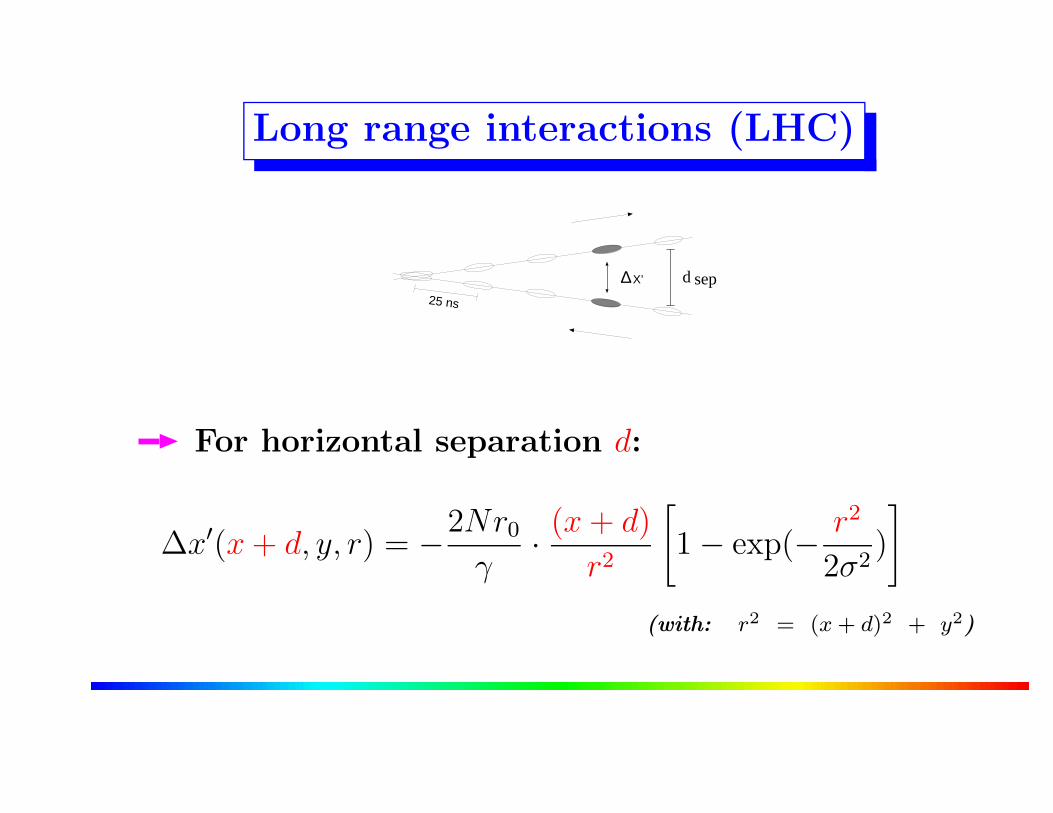
Long range interactions (LHC)
∆X’ d sep25 ns
For horizontal separation d:
∆x′(x + d, y, r) = −2Nr0
γ· (x + d)
r2
[
1 − exp(− r2
2σ2)
]
(with: r2 = (x + d)2 + y2)
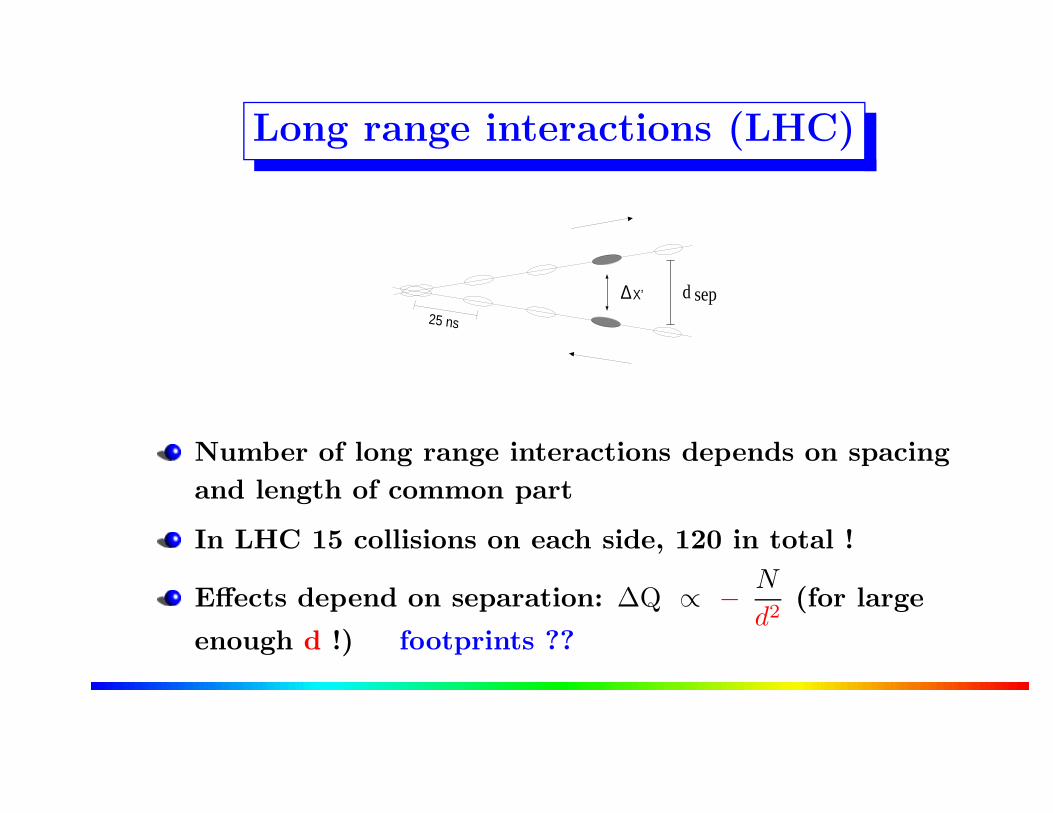
Long range interactions (LHC)
∆X’ d sep25 ns
Number of long range interactions depends on spacing
and length of common part
In LHC 15 collisions on each side, 120 in total !
Effects depend on separation: ∆Q ∝ − N
d2(for large
enough d !) footprints ??
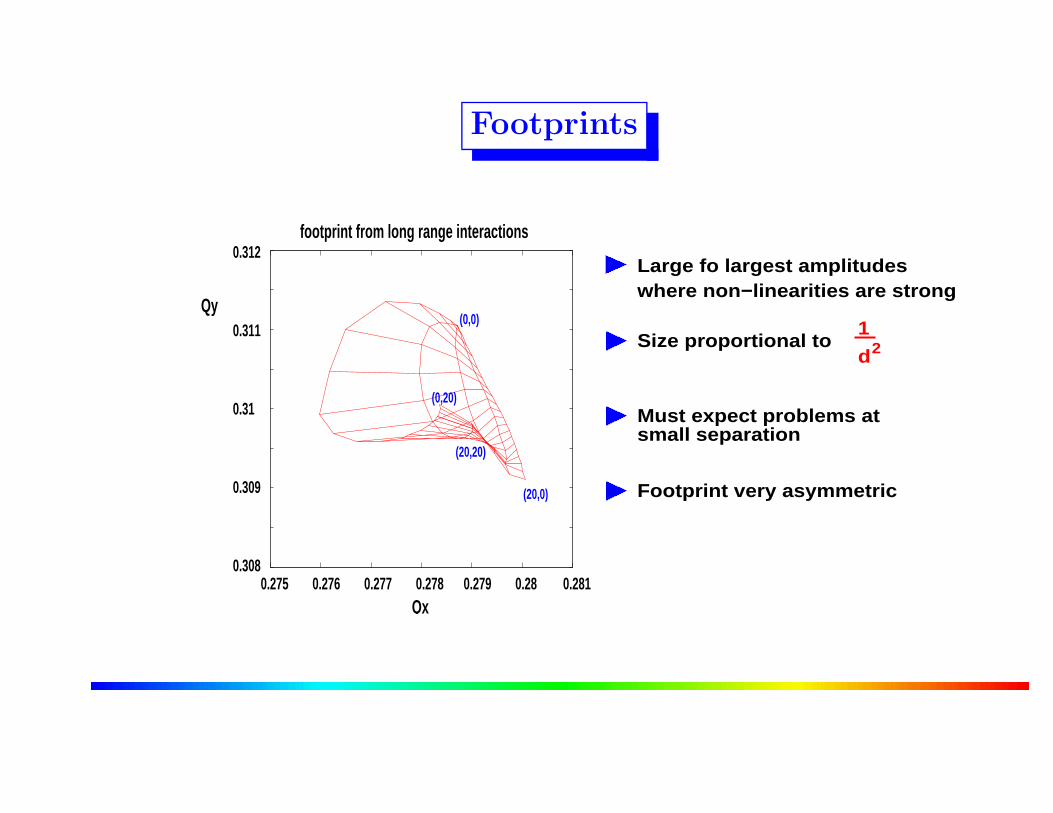
Footprints
footprint from long range interactions
Qy
0.312
0.311
0.31
0.309
0.3080.275 0.276 0.277 0.278 0.279 0.28 0.281
Qx
(0,0)
(20,0)
(0,20)
(20,20)
1
d2
� � �� � �� � �� � �� � �� �� �� �
� �� �� �� �� �� ��� �� �� �� �
� �� �� �� �� �� �� �� �� �� �
� �� �� �� ��� �� �� �� �
where non−linearities are strong
Footprint very asymmetric
Must expect problems atsmall separation
Size proportional to
Large fo largest amplitudes

Particle losses
Small crossing angle ⇐⇒ small separation
Small separation: particles become unstable and get lost
Minimum crossing angle for LHC: 285 µrad

Closed orbit effects
∆x′(x + d, y, r) = −2Nr0
γ· (x + d)
r2
[
1 − exp(− r2
2σ2)
]
For well separated beams (d � σ) the force (kick) has an
amplitude independent contribution: orbit kick
∆x′ =const.
d· [ 1
︸ ︷︷ ︸
− x
d+ O
(x2
d2
)
+ ...
∆ X’

Closed orbit effects
Beam-beam kick from long range interactions
changes the orbit
Has been observed in LEP with bunch trains
Self-consistent calculation necessary
Effects can add up and become important
Orbit can be corrected, but:
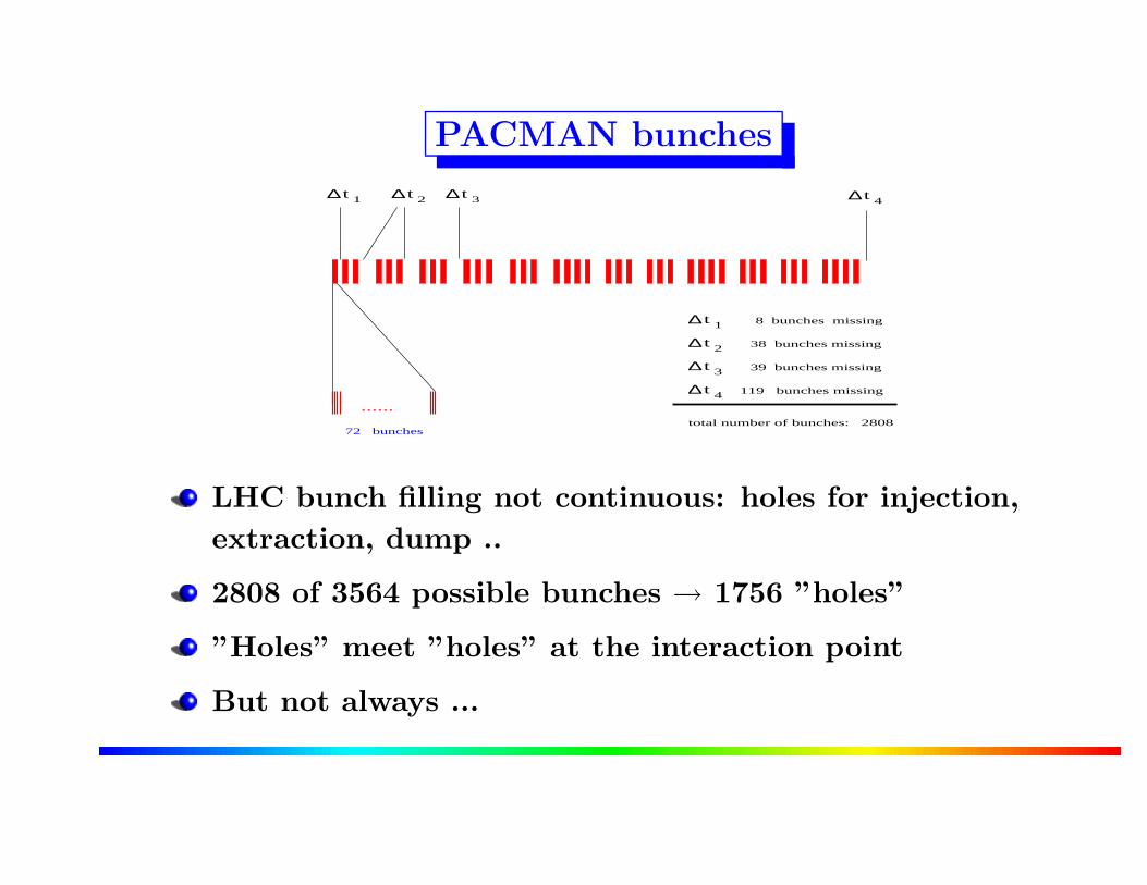
PACMAN bunches
......
72 bunches
∆ t 3∆ t 2 ∆ t 1
∆ t 1
∆ t 2
∆ t 3
∆ t 4
8 bunches missing
38 bunches missing
119 bunches missing
total number of bunches: 2808
39 bunches missing
∆ t 4
LHC bunch filling not continuous: holes for injection,
extraction, dump ..
2808 of 3564 possible bunches → 1756 ”holes”
”Holes” meet ”holes” at the interaction point
But not always ...
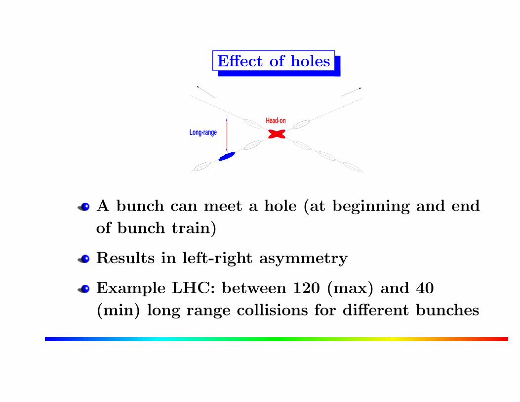
Effect of holes
� � � � � �
� � � � � �
� � � � � �
� � � � � �
� � � � � �
� � � � � �
� � � � � �
� � � � � �
Head-onLong-range
A bunch can meet a hole (at beginning and end
of bunch train)
Results in left-right asymmetry
Example LHC: between 120 (max) and 40
(min) long range collisions for different bunches

PACMAN bunches
When a bunch meets a ”hole”:
Miss some long range interactions, PACMAN
bunches
They see fewer unwanted interactions in total
Different integrated beam-beam effect
Example: orbit and tune effects

Orbit along batches: beam 1
-2
-1
0
1
2
0 50 100 150 200 250
orbi
t (m
icro
n)
Bunch number along bunch train
Orbit along bunches Orbit beam 1
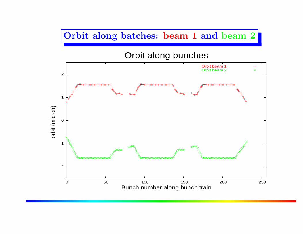
Orbit along batches: beam 1 and beam 2
-2
-1
0
1
2
0 50 100 150 200 250
orbi
t (m
icro
n)
Bunch number along bunch train
Orbit along bunches Orbit beam 1 Orbit beam 2

Tune along batches
0.306
0.308
0.31
0.312
0.314
0 50 100 150 200 250
Hor
izon
tal t
une
Bunch number along bunch train
Tune along bunches Qx spread for bunches in beam 1
Spread is too large for safe operation
Beam-beam deflection scan
The orbit effect can be useful when one has
only a few bunches, i.e. not PACMAN effects
Effect can be used to optimize luminosity
Scanning two beams against each other
Two beams get a orbit kick, depending on
distance
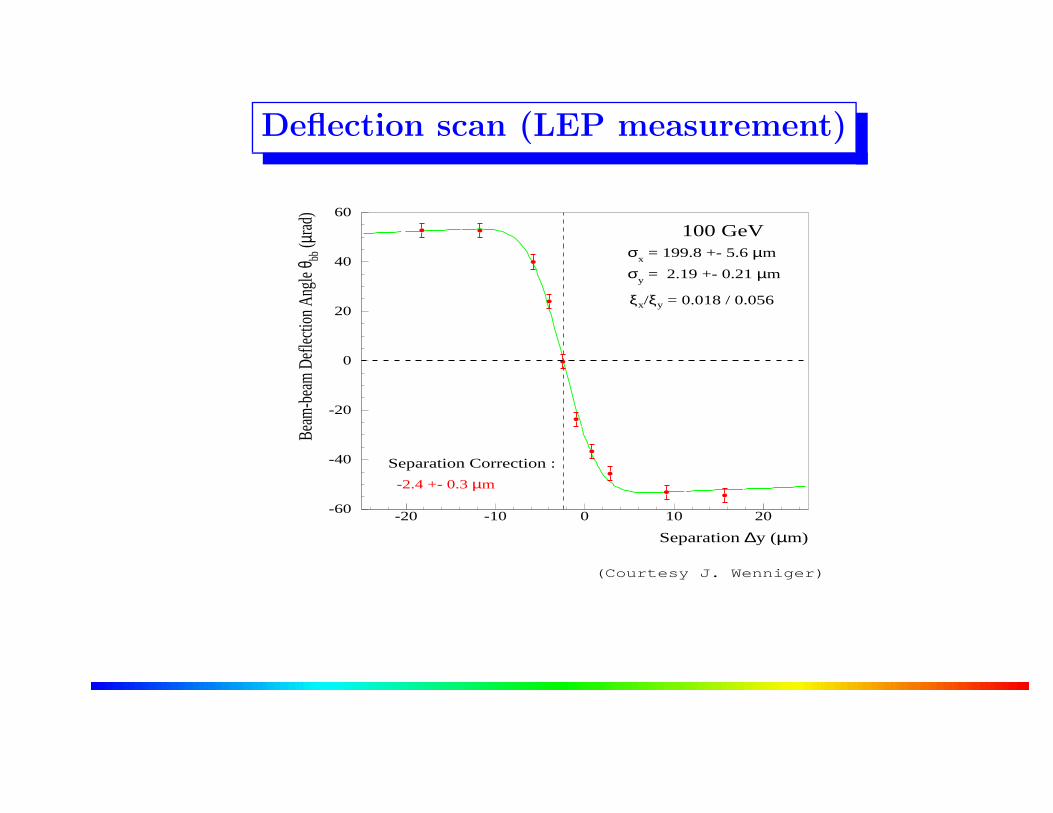
Deflection scan (LEP measurement)
-60
-40
-20
0
20
40
60
-20 -10 0 10 20
Separation ∆y (µm)
Beam
-bea
m D
eflec
tion
Angl
e θbb
(µra
d)
100 GeV
Separation Correction :
-2.4 +- 0.3 µm
σx = 199.8 +- 5.6 µm
σy = 2.19 +- 0.21 µm
ξx/ξy = 0.018 / 0.056
(Courtesy J. Wenniger)
Deflection scan
Calculated kick from orbit follows the force
function
Allows to calculate parameters
Allows to centre the beam
Standard procedure at LEP
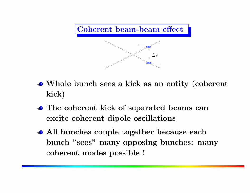
Coherent beam-beam effect
∆ X’
Whole bunch sees a kick as an entity (coherent
kick)
The coherent kick of separated beams can
excite coherent dipole oscillations
All bunches couple together because each
bunch ”sees” many opposing bunches: many
coherent modes possible !
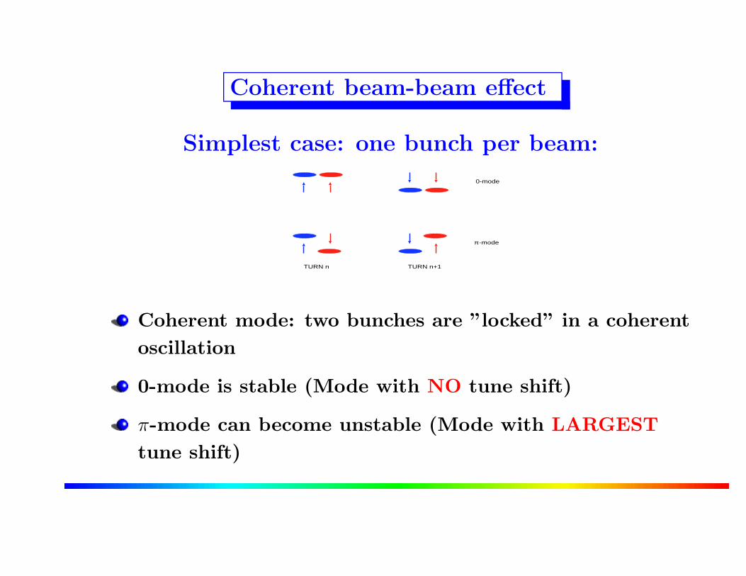
Coherent beam-beam effect
Simplest case: one bunch per beam:
0-mode
π -mode
TURN n TURN n+1
Coherent mode: two bunches are ”locked” in a coherent
oscillation
0-mode is stable (Mode with NO tune shift)
π-mode can become unstable (Mode with LARGEST
tune shift)
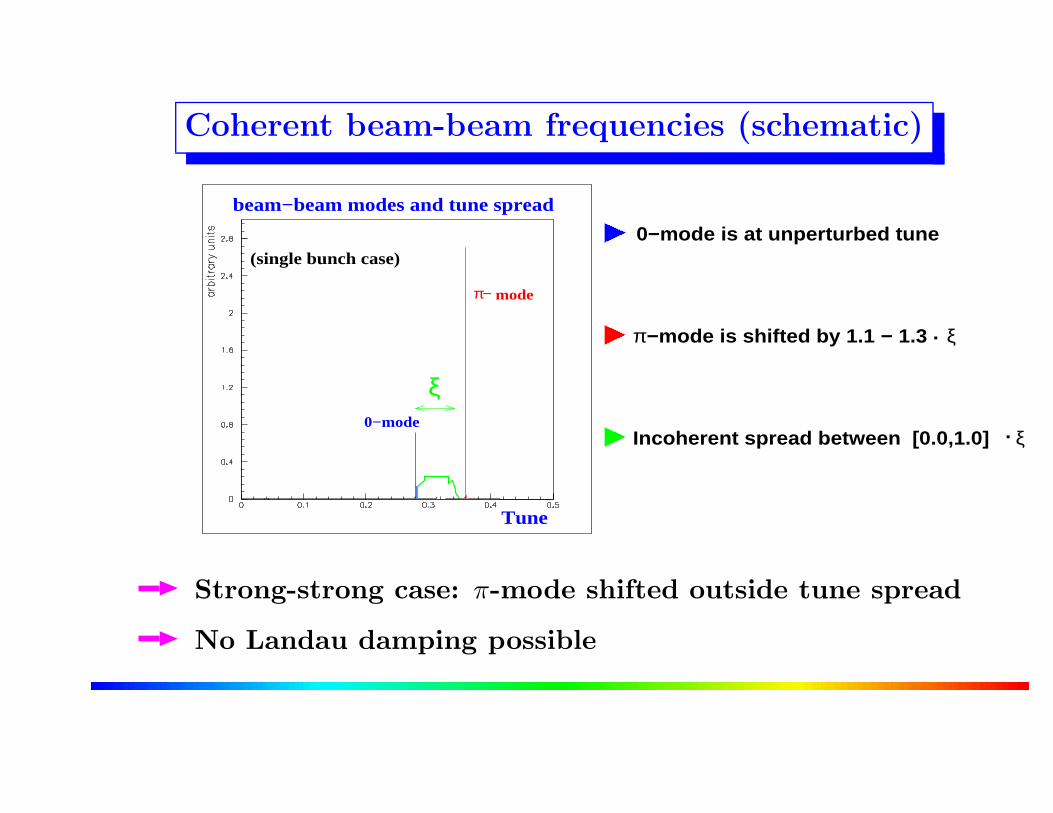
Coherent beam-beam frequencies (schematic)
π− mode
0−mode
Tune
(single bunch case)
beam−beam modes and tune spread
ξ
� � �� � �� � �� � �� � �
� � �� � �� � �� � �
� � �� � �� � �� � �
� � �� � �� � �� � �
� � �� � �� � �� � �
� � �� � �� � �� � �
0−mode is at unperturbed tune
π−mode is shifted by 1.1 − 1.3
Incoherent spread between [0.0,1.0]
ξ.
. ξ
Strong-strong case: π-mode shifted outside tune spread
No Landau damping possible

Measurement: LEP
0
0.002
0.004
0.006
0.008
0.01
0.012
0.2 0.21 0.22 0.23 0.24 0.25 0.26 0.27 0.28 0.29 0.3 0.31 0.32 0.33 0.34 0.35 0.36 0.37 0.38 0.39 0.4Qx
’Q_FFT_TfsQ2_99_10_19:07_26_25’ u 2:4
Two modes clearly visible
Can be distinguished by phase relation, i.e.
sum and difference signals
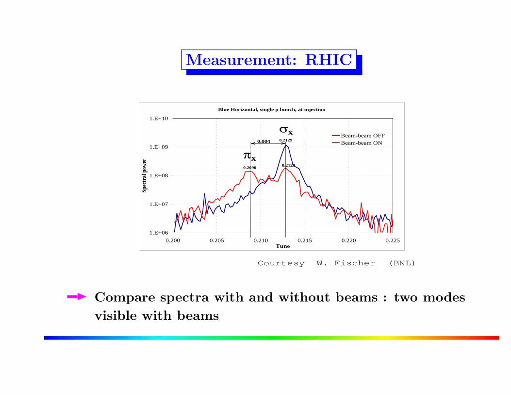
Measurement: RHIC
Blue Horizontal, single p bunch, at injection
0.2129
0.20900.2129
1.E+06
1.E+07
1.E+08
1.E+09
1.E+10
0.200 0.205 0.210 0.215 0.220 0.225Tune
Spec
tral
pow
erBeam-beam OFF
Beam-beam ON
SSx
VVx0.004
Courtesy W. Fischer (BNL)
Compare spectra with and without beams : two modes
visible with beams

Simulation of coherent spectra
Coherent modes, Hybrid Fast Multipole Method
0
0.1
0.2
0.3
0.4
0.5
0.6
0.7
0.8
-2 -1.5 -1 -0.5 0 0.5
� � �
� � �
� � �
� � �
� � �
� � �
� � �
� � �
� � �
� � �
� � �
� � �
� � �
� � �
� � �
� � �
� � �
� � �
� � �
� � �
� � �
� � �
� � �
� � �
� � �
� � �
� � �
� � �
� � �
� � �
� � �
� � �
� � �
� � �
Full simulation of both beams required
Use up to 10 particles in simulations
Requires computation of arbitrary fields
8
Must take into account changing fields

Many bunches and more interaction points
0
5
10
15
20
25
30
35
40
0.29 0.295 0.3 0.305 0.31 0.315 0.32
S(Q
x)
horizontal tune
36 bunches, 2 unsymmetric interaction points
Bunches couple via the beam-beam interaction
Additional coherent modes become visible
Potentially undesirable situation

What can be done to avoid problems ?
Coherent motion requires ’organized’ motion of
many particles
Therefore high degree of symmetry required
Possible countermeasure: (symmetry breaking)
→ Different bunch intensity
→ Different tunes in the two beams
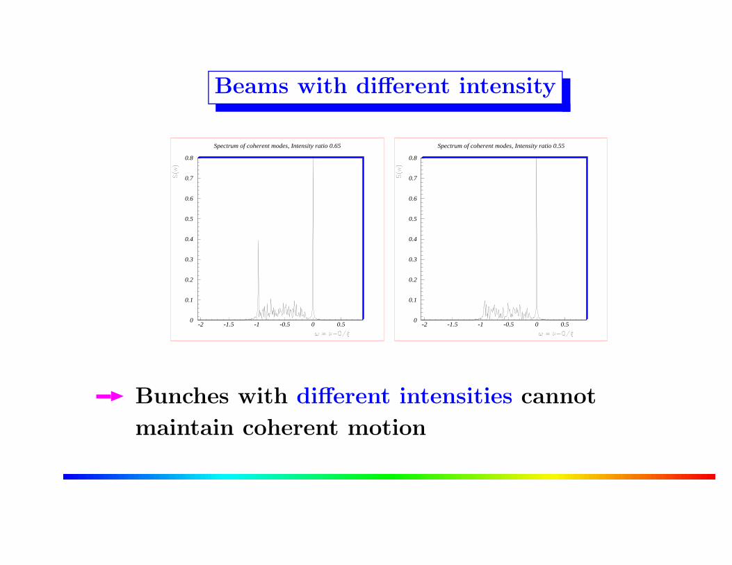
Beams with different intensity
Spectrum of coherent modes, Intensity ratio 0.65
0
0.1
0.2
0.3
0.4
0.5
0.6
0.7
0.8
-2 -1.5 -1 -0.5 0 0.5
Spectrum of coherent modes, Intensity ratio 0.55
0
0.1
0.2
0.3
0.4
0.5
0.6
0.7
0.8
-2 -1.5 -1 -0.5 0 0.5
Bunches with different intensities cannot
maintain coherent motion
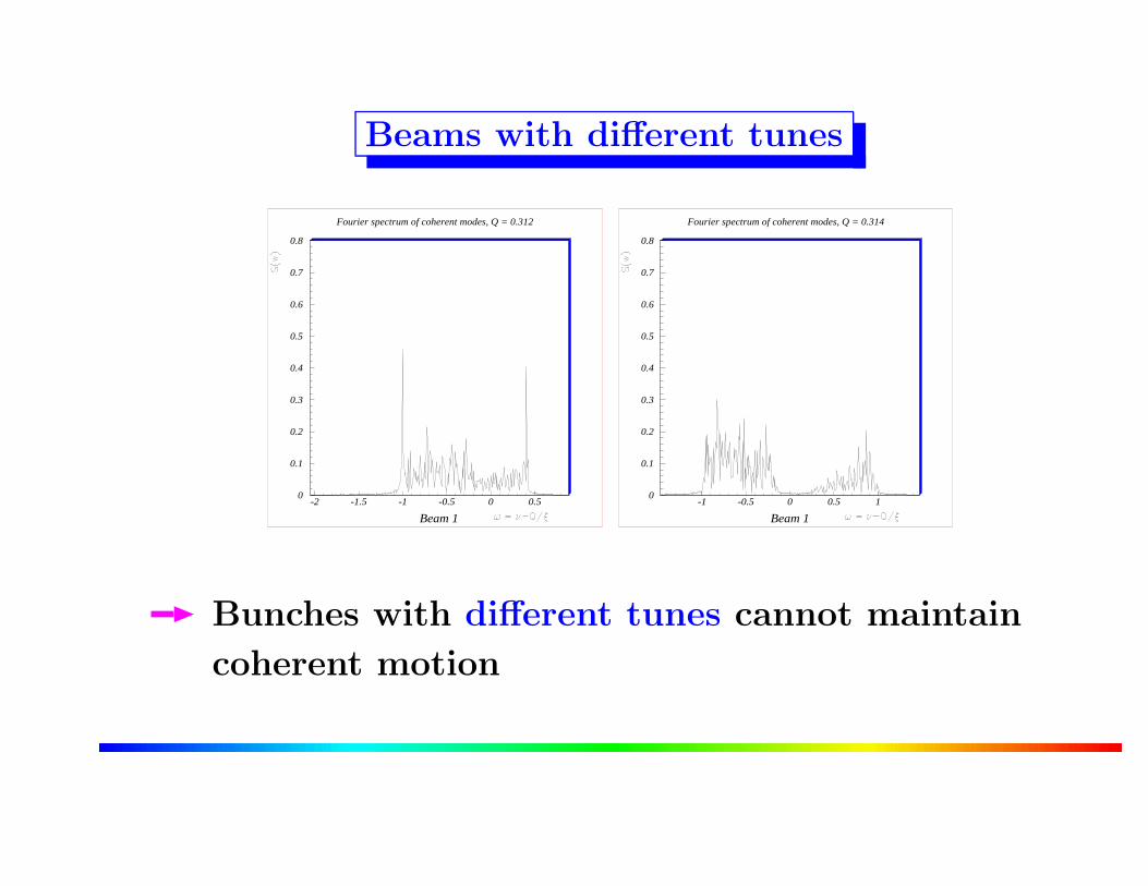
Beams with different tunes
Fourier spectrum of coherent modes, Q = 0.312
0
0.1
0.2
0.3
0.4
0.5
0.6
0.7
0.8
-2 -1.5 -1 -0.5 0 0.5
Beam 1
Fourier spectrum of coherent modes, Q = 0.314
0
0.1
0.2
0.3
0.4
0.5
0.6
0.7
0.8
-1 -0.5 0 0.5 1
Beam 1
Bunches with different tunes cannot maintain
coherent motion
Can we suppress beam-beam effects ?
Find ’lenses’ to correct beam-beam effects
Head on effects:
→ Linear ”electron lens” to shift tunes
→ Non-linear ”electron lens” to reduce spread
→ Tests in progress at FNAL
Long range effects:
→ At very large distance: force is 1/r
→ Same force as a wire !
So far: mixed success with active compensation

Others: Mobius lattice
Principle:
→ Interchange horizontal and vertical plane
each turn
Effects:
→ Round beams (even for leptons)
→ Some compensation effects for beam-beam
interaction
→ First test at CESR at Cornell
Not mentioned:
Effects in linear colliders
Asymmetric beams
Coasting beams
Beamstrahlung
Synchrobetatron coupling
Monochromatization
Beam-beam experiments
... and many more
Bibliography
Some bibliography in the hand-out
Beam-beam lectures:A. Chao, The beam-beam instability, SLAC-PUB-3179 (1983).
L. Evans, The beam-beam interaction, CAS Course on proton-antiproton
colliders, in CERN 84-15 (1984).
L. Evans and J. Gareyte, Beam-beam effects, CERN Accelerator School, Oxford
1985, in: CERN 87-03 (1987).
A. Zholents, Beam-beam effects in electron-positron storage rings, Joint
US-CERN School on Particle Accelerators, in Springer, Lecture Notes in
Physics, 400 (1992).
Beam-beam force:E. Keil, Beam-beam dynamics, CERN Accelerator School, Rhodes 1993, in:
CERN 95-06 (1995).
M. Basetti and G.A. Erskine, Closed expression for the electrical field of a
2-dimensional Gaussian charge, CERN-ISR-TH/80-06 (1980).
PACMAN bunches:W. Herr, Effects of PACMAN bunches in the LHC, CERN LHC Project
Report 39 (1996).
Coherent beam-beam effects:A. Piwinski, Observation of beam-beam effects in PETRA, IEEE Trans. Nucl.
Sc., Vol.NS-26 4268 (1979).
K. Yokoya et al., Tune shift of coherent beam-beam oscillations, Part. Acc. 27,
181 (1990).
Y. Alexahin, On the Landau damping and decoherence of transverse dipole
oscillations in colliding beams, Part. Acc. 59, 43 (1996).
A. Chao, Coherent beam-beam effects, SSC Laboratory, SSCL-346 (1991).
Y. Alexahin, A study of the coherent beam-beam effect in the framework of the
Vlasov perturbation theory, Nucl. Inst. Meth. A 380, 253 (2002).
Y. Alexahin, H. Grote, W. Herr and M.P. Zorzano, Coherent beam-beam
effects in the LHC, CERN LHC Project Report 466 (2001).
Simulations (incoherent beam-beam):W. Herr, Computational Methods for beam-beam interactions, incoherent
effects, Lecture at CAS, Sevilla 2001,
at http://cern.ch/lhc-beam-beam/talks/comp1.ps.
Simulations (coherent beam-beam):W. Herr, Computational Methods for beam-beam interactions, coherent effects,
Lecture at CAS, Sevilla 2001,
at http://cern.ch/lhc-beam-beam/talks/comp2.ps.
W. Herr, M.P. Zorzano, and F. Jones, A hybrid fast multipole method applied
to beam-beam collisions in the strong-strong regime, Phys. Rev. ST Accel.
Beams 4, 054402 (2001).
W. Herr and R. Paparella, Landau damping of coherent modes by overlap with
synchrotron sidebands, CERN LHC Project Note 304 (2002).
Mobius accelerator:R. Talman, A proposed Mobius accelerator, Phys. Rev. Lett. 74, 1590 (1995).


![Cern Accelerator School Talk [Kompatibilitätsmodus]cas.web.cern.ch/sites/cas.web.cern.ch/files/... · Complex multiphysics circuit analysis: AC, DC and TR analysis Based on numerical](https://static.fdocuments.in/doc/165x107/5ebecb9bcc3168067439e702/cern-accelerator-school-talk-kompatibilittsmoduscaswebcernchsitescaswebcernchfiles.jpg)


