B.COM 104- Micro Economics- I Course Contents Unit I Introduction to Economics and Demand Theory: Opportunity cost and marginalism- production possibility frontier, Law of demand and consumer equilibrium-cardinal utility approach: Indifference Curve-price income and substitution effect. Unit II Demand, Supply and the Markets, Demand Curves: Individual demand curves and market demand curve, movement along Vs shift market demand curve. Elasticity of demand-nature and types of theory of supply, law of supply, equilibrium supply curves, elasticity of supply, shifts in demand and supply, shifts in demand and supply. Unit III Theory of Production: Meaning and Concept of Production, Factors of Production and Production function, Fixed and Variable Factors, Law of Variable Proportion (Short Run Production Analysis), Law of Returns to a Scale (Long Run Production Analysis) through the use of ISO QUANTS. Unit IV Cost Analysis & Price Output Decisions: Concept of Cost, Cost Function, Short Run Cost, Long Run Cost, Economies and Diseconomies of Scale, Explicit Cost and Implicit Cost, Private and Social Cost; Revenue: concept, types, revenue curves.

UNIT-1 ECONOMICS: The social science that deals with the production, distribution, and consumption of goods and services and with the theory and management of economies or economic systems. The word ‘Economics’ originates from the Greek work ‘Oikonomikos’ which can be divided

into two parts: (a) ‘Oikos’, which means ‘Home’, and

(b) ‘Nomos’, which means ‘Management’. Thus, Economics means ‘Home Management’. The head of a family faces the problem of managing the unlimited wants of the family members within the limited income of the family. In fact, the same is true for a society also. If we consider the whole society as a ‘family’, then the society also faces the problem of tackling unlimited wants of the members of the society with the limited resources available in that society. Thus, Economics means the study of the way in which mankind organizes itself to tackle the basic problems of scarcity. All societies have more wants than resources. Hence, a system must be devised to allocate these resources between competing ends.

DEFINITION OF ECONOMICS

Definitions of Economics can be classified into four groups:

1. Wealth definitions, 2. Material welfare definitions,

3. Scarcity definitions, and 4. Growth-centered definitions.

Adam Smith’s Definition Adam Smith considered to be the founding father of modern Economics, defined Economics as the study of the nature and causes of nations’ wealth or simply as the study of wealth. The central point in Smith’s definition is wealth creation He assumed that, the wealthier a nation becomes the happier are its citizens. Thus, it is important to find out, how a nation can be wealthy. Economics is the subject that tells us how to make a nation wealthy. Adam Smith’s definition is a wealth-centered definition of Economics.

Alfred Marshall’s Definition Alfred Marshall also stressed the importance of wealth. But he also emphasized the role of the individual in the creation and the use of wealth. He wrote: “Economics is a study of man in the ordinary business of life. It enquires how he gets his income and how he uses it. Thus, it is on the one side, the study of wealth and on the other and more important side, a part of the study of man”. Marshall, therefore, stressed the supreme importance of man in the economic system. Marshall’s definition is considered to be material-welfare centered definition of Economics.

Lionel Robbins’ Definition The next important definition of Economics was due to Prof. Lionel Robbins. According to Robbins, “Economics is a science which studies human behaviour as a relationship between ends and scarce means which have alternative uses”. It is a scarcity-based definition of Economics.

Growth-Oriented Definition of Samuelson Professor Samuelson writes, “Economics is the study of how people and society end up choosing, with or without the use of money, to employ scarce productive resources that could have alternative uses to produce various commodities over time and distributing them for consumption, now or in the future, among various persons or groups in society. It analyses costs and benefits of improving patterns of resource allocation”

DIFFERENCE BETWEEN MICRO AND MACRO ECONOMICS

Micro Economics 1. Evolution of micro economics took place earlier than macro economics. 2. It deals with an individual's economic behavior. 3. It is a branch of economics, which studies individual economic variables like demand, supply, price

etc. 4. It has a very narrow scope i.e. an individual, a market etc. 5. Demand, supply, market forms etc. relate to micro economics. 6. It is helpful in analysis of an individual economics unit like firm. 7. Theory of demand, theory of production, price determination theory etc., develop from micro

economics. 8. The concepts of micro-economics are independent concepts. 9. These concepts have more theoretical value. 10. The concepts were popularized by the famous Alfred Marshall. 11. Worm’s eye view/ Microscopic view 12. Method of Slicing 13. It is a mortal concept 14. Simple 15. Price Theory

Macro Economics 1. It evolved only after the publication of keynes' book. General theory of employment, interest and

money. 2. It deals with aggregate economic behavior of the people in general. 3. It is a branch of economics which studies aggregate economic variables, like aggregate demand,

aggregate supply, price level etc. 4. It has a very wide scope i.e. a country. 5. Aggregate demand, aggregate supply, national income etc. relate to macro economics. 6. It is helpful for analyzing the level of employment, income, economic growth etc.

7. Theory of national income, theory of employment, theory of money, theory of general price level

etc. develop from macro economics. 8. The concepts of macro economics are interdependent on one another. 9. These concepts have more practical value. 10. The concepts were popularized by the famous Lord J.M. Keynes. 11. Bird’s eye view 12. Method of Lumping 13. It is an immortal concept 14. Complex 15. Income theory

OPPORTUNITY COST A benefit, profit, or value of something that must be given up to acquire or achieve something else. Since every resource (land, money, time, etc.) can be put to alternative uses, every action, choice, or decision has an associated opportunity cost.

Opportunity costs are fundamental costs in economics, and are used in computing cost benefit analysis of a project. Such costs, however, are not recorded in the account books but are recognized in decision making by computing the cash outlays and their resulting profit or loss.

“The cost of passing up the next best alternate choice while making a decision.” For example, if an asset such as capital is used for one purpose, the opportunity cost is the value of the next best purpose the asset could have been used for. Opportunity cost analysis is an important part of a company's decision-making processes, but is not treated as an actual cost in any financial statement.

Production Possibility Curve A graphical representation of the alternative combinations of the amounts of two goods or services that an economy can produce by transferring resources from one good or service to the other. It is also called transformation curve. The Production Possibilities Curve (PPC) models a two-good economy by mapping production of one good on the x-axis and production of the other good on the y-axis. The combinations of outputs produced using the best technology and all available resources make up the PPC. Points inside the PPC result from inefficiency; output combinations outside the PPC are impossible to produce. The guns and butter PPC, for example, illustrates tradeoffs between producing goods for peaceful and military purposes. This PPC illustrates opportunity cost in that more guns cannot be produced without reducing butter output; further, the slope of the PPC indicates the nature of the tradeoff between guns and butter (that is, how many guns must be given up to obtain an additional ton of butter).

Marginalism In economics, marginalism is the theory that economic value results from marginal utility and marginal cost (the marginal concepts). Marginalism is the notion that what is most important for decision making is the marginal or last unit of consumption or production.

DEMAND Demand is defined as the quantity of a good or service that consumers are willing and able to buy at a given price in a given time period. Each of us has an individual demand for particular goods and services and the level of demand at each market price reflects the value that consumers place on a product and their expected satisfaction gained from purchase and consumption.

The Law of Demand “Other factors remaining constant (ceteris paribus) there is an inverse relationship between the price of a good and demand.” As prices fall, we see an expansion of demand, If price rises, there will be a contraction of demand.

A change in the price of a good or service causes a movement along the demand curve:

Many other factors can affect total demand - when these change, the demand curve can shift. This is explained below. Shifts in the Demand Curve Caused by Changes in the Conditions of Demand

There are two possibilities: either the demand curve shifts to the right or it shifts to the left.

Demand Curve In economics, the demand curve is the graph depicting the relationship between the price of a certain commodity and the amount of it that consumers are willing and able to purchase at that given price. It is a graphic representation of a demand schedule. The demand curve for all consumers together follows from the demand curve of every individual consumer: the individual demands at each price are added together.

Factors affecting market demand Market or aggregate demand is the summation of individual demand curves. In addition to the factors which can affect individual demand there are three factors that can affect market demand (cause the market demand curve to shift):

• a change in the number of consumers, • a change in the distribution of tastes among consumers,

• a change in the distribution of income among consumers with different tastes. Some circumstances which can cause the demand curve to shift in include:

• Decrease in price of a substitute • Increase in price of a complement

• Decrease in income if good is normal good • Increase in income if good is inferior good

Exceptions to the Law of Demand The law of demand does not apply in every case and situation. The circumstances when the law of demand becomes ineffective are known as exceptions of the law. Some of these important exceptions are as under.

(1) Prestige goods. There are certain commodities like diamond, sports, cars etc., which are purchased as a mark of distinction in society. If the price of these goods rise, the demand for them may increase instead of falling. (2) Price expectations. If people expect a further rise in the price of a particular commodity, they may buy more inspite of rise in price: The violation of the law in this case is only temporary. (3) Ignorance of the consumer. If, the Consumer is ignorant *about the rise in price of goods, he may buy more at a higher price. (4) Giffen goods. If the prices of basic goods, (potatoes, bajra, sugar etc) on which the poor spend a large part of their incomes declines, the poor increase the demand for superior goods, hence when the price of Giffen good falls, its demand also falls. There is a positive price effect in the case of Giffen goods.

(5) Veblen Goods. Another exception is based on the doctrine of conspicuous consumption attributed by Thorstein Veblen. People purchase certain goods for ostentation or showy purposes. Such goods are known as Veblen goods. Since these goods are used to impress others, people may not buy when the price falls. In other words, demand decreases when the price falls.

(6) Snob Effect. Some buyers have a desire to own unusual or unique products to show that they are different from others.

CONSUMER EQUILIBRIUM Theory of Consumer’s Behavior: Utility Analysis The theory of consumer’s behavior seeks to explain the determination of consumer’s equilibrium. Consumer’s equilibrium refers to a situation when a consumer gets maximum satisfaction out of his given resources. A consumer spends his money income on different goods and services in such a manner as to derive maximum satisfaction. Once a consumer attains equilibrium position, he would not like to deviate from it. Economic theory has approached the problem of determination of consumer’s equilibrium in two different ways: (1) Cardinal Utility Analysis and (2) Ordinal Utility Analysis Accordingly, we shall examine these two approaches to the study of consumer’s equilibrium in greater defeat.

Meaning of Utility: The term utility in Economics is used to denote that quality in a good or service by virtue of which our wants are satisfied. In, other words utility is defined as the want satisfying power of a commodity. According to, Mrs. Robinson, “Utility is the quality in commodities that makes individuals want to buy them.”

According to Hibdon, “Utility is the quality of a good to satisfy a want.”

Concepts of Utility There are three concepts of utility :

(1) Initial Utility: The utility derived from the first unit of a commodity is called initial utility. Utility derived from the first piece of bread is called initial utility. Thus, initial utility, is the utility obtained from the consumption of the first unit of a commodity. It is always positive. (2) Total Utility: Total utility is the sum of utility derived from different Units of a commodity consumed by a household. According to Leftwitch, “Total utility refers to the entire amount of satisfaction obtained from consuming various quantities of a commodity.” Suppose a consumer consume four units of apple. If the consumer gets 10 utils from the consumption of first apple, 8 utils from second, 6 utils from third, and 4 utils from fourth apple, then the total utility will be 10+8+6+4 = 28 Accordingly, total utility can be calculated as :

TU = MU1 + MU2 + MU3 + _________________ + MUn Or

TU = ∑MU

Here TU = Total utility and MU1, MU2, MU3, + __________ MUn = Marginal Utility derived from first, second, third __________ and nth unit.

(3) Marginal Utility: Marginal Utility is the utility derived from the additional unit of a commodity consumed. The change that takes place in the total utility by the consumption of an additional unit of a commodity is called marginal utility. According to Chapman, “Marginal utility is the addition made to total utility by consuming one more unit of commodity. Supposing a consumer gets 10 utils from the consumption of one mango and 18 utils from two mangoes, then. the marginal utility of second .mango will be 18-10=8 utils. Marginal utility can be measured with the help of the following formula MUnth = TUn – TUn-1

Here MUnth = Marginal utility of nth unit, TUn = Total utility of ‘n’ units,

TUn-l = Total utility of n-i units, Marginal utility can be (i) positive, (ii) zero, or (iii) negative.

(i) Positive Marginal Utility: If by consuming additional units of a commodity, total utility goes on increasing, marginal utility will be positive.

(ii) Zero Marginal Utility: If the consumption of an additional unit of a commodity causes no change in total utility, marginal utility will be zero.

(iii) Negative Marginal Utility: If the consumption of an additional unit of a commodity causes fall in total utility, the marginal utility will be negative.

Utility Analysis or Cardinal Approach

The Cardinal Approach to the theory of consumer behavior is based upon the concept of utility. It assumes that utility is capable of measurement. It can be added, subtracted, multiplied, and so on. According to this approach, utility can be measured in cardinal numbers, like 1,2,3,4 etc. Fisher has used the term ‘Util’ as a measure of utility. Thus in terms of cardinal approach it can be said that one gets from a cup of tea 5 utils, from a cup of coffee 10 utils, and from a rasgulla 15 utils worth of utility.

Laws of Utility Analysis Utility analysis consists of two important laws

1. Law of Diminishing Marginal Utility. 2. Law of Equi-Marginal Utility.

1. Law of Diminishing Marginal Utility : Law of Diminishing Marginal Utility is an important law of utility analysis. This law is related to the satisfaction of human wants. All of us experience this law in our daily life. If you are set to buy, say, shirts at any given time, then as the number of shirts with you goes on increasing, the

marginal utility from each successive shirt will go on decreasing. It is the reality of a man’s life which is referred to in economics as law of Diminishing Marginal Utility. This law is also known as Gossen’s First Law. According to Chapman, “The more we have of a thing, the less we want additional increments of it or the more we want not to have additional increments of it.” According to Marshall, “The additional benefit which a person derives from a given stock of a thing diminishes with every increase in the stock that he already has.” According to Samuelson, “As the amount consumed of a good increases, the marginal utility of the goods tends to decrease.” In short, the law of Diminishing Marginal Utility states that, other things being equal, when we go on consuming additional units of a commodity, the marginal utility from each successive unit of that commodity goes on diminishing.

Assumptions: Every law in subject to clause “other things being equal” This refers to the assumption on which a law is based. It applies in this case as well. Main assumptions of this law are as follows:

1. Utility can be measured in cardinal number system such as 1,2,3_______ etc.

2. There is no change in income of the consumer. 3. Marginal utility of money remains constant.

4. Suitable quantity of the commodity is consumed. 5. There is continuous consumption of the commodity.

6. Marginal Utility of every commodity is independent. 7. Every unit of the commodity being used is of same quality and size.

8. There is no change in the tastes, character, fashion, and habits of the Consumer. 9. There is no change in the price of the commodity and its substitutes.

ORDINAL UTILITY Ordinal utility theory states that while the utility of a particular good or service cannot be measured using a numerical scale bearing economic meaning in and of itself, pairs of alternative bundles (combinations) of goods can be ordered such that one is considered by an individual to be worse than, equal to, or better than the other. This contrasts with cardinal utility theory, which generally treats utility as something whose numerical value is meaningful in its own right. The concept was first introduced by Pareto in 1906

Ordinal utility Definition: A method of analyzing utility, or satisfaction derived from the consumption of goods and services, based on a relative ranking of the goods and services consumed. With ordinal utility, goods are only ranked only in terms of more or less preferred, there is no attempt to determine

how much more one good is preferred to another. Ordinal utility is the underlying assumption used in the analysis of indifference curves and should be compared with cardinal utility, which (hypothetically) measures utility using a quantitative scale.

Indifference Curve Approach An indifference curve is a geometrical presentation of a consumer is scale of preferences. It represents all those combinations of two goods which will provide equal satisfaction to a consumer. A consumer is indifferent towards the different combinations located on such a curve. Since each combination yields the same level of satisfaction, the total satisfaction derived from any of these combinations remains constant. An indifference curve is a locus of all such points which shows different combinations of two commodities which yield equal satisfaction to the consumer. Since the combination represented by each point on the indifference curve yields equal satisfaction, a consumer becomes indifferent about their choice. In other words, he gives equal importance to all the combinations on a given indifference curve. According to ferguson, “An indifference curve is a combination of goods, each of which yield the same

level of total utility to which the consumer is indifferent.”

Indifference Schedule An indifference schedule refers to a schedule that indicates different combinations of two commodities which yield equal satisfaction. A consumer, therefore, gives equal importance to each of the combinations. Suppose a consumer two goods, namely apples and oranges. The following indifference schedule indicates different combinations of apples and oranges that yield him equal satisfaction.

Combination of Apple Oranges

Apple Oranges

A 1 0

B 2 7

C 3 5

D 4 4

Assumptions: Indifference curve approach has the following main assumptions:

1. Rational Consumer: It is assumed that the consumer will behave rationally. It means the consumer would like to get maximum satisfaction out of his total income.

2. Diminishing Marginal rate of Substitution: It means as the stock of a commodity increases with the consumer, he substitutes it for the other commodity at a diminishing rate.

3. Ordinal Utility: A consumer can determine his preferences on the basis of satisfaction derived from different goods or their combinations. Utility can be expressed in terms of ordinal numbers, i.e., first, second etc.

4. Independent Scale of Preference: It means if the income of the consumer changes or prices of goods fall or rise in the market, these changes will have no effect on the scale of preference of the consumer. It is further assumed that scale of preference of a consumer is not influenced by the scale of preference of another consumer.

5. Non-Satiety: A consumer does not possess any good in more than the required quantity. He does not reach the level of satiety. Consumer prefers more quantity of a good to less quantity.

6. Consistency in Selection: There is a consistency in consumer’sbehaviour. It means that if at any given time a consumer prefers A combination of goods to B combination, then at another time he will not prefer B combination to A combination.

7. Transitivity: It means if a consumer prefers A combination to B combination, and B Combination to C Combination, he will definitely prefer A combination to C combination. Likewise; if a consumer is indifferent towards A and B and he is also indifferent towards Band C, then he will also he indifferent towards A and C.

Properties of Indifference Curves 1. Indifference curve slopes downward from left to right, or an indifference curve has a negative

slope

2. Indifference curve is convex to the point of origin: 3. Two Indifference Curves never cut each other:

4. Higher Indifference Curves represent more satisfaction 5. Indifference Curve touches neither x-axis nor y-axis;

6. Indifference curves need not be parallel to each other: 7. Indifference curves become complex in case of more than two commodities

PRICE EFFECT Price effect represents change in consumer’s optimal consumption combination on account of change in the price of a good and thereby changes in its quantity purchased, price of another good and consumer’s income remaining unchanged. The consumer is better-off when optimal consumption combination is located on a higher indifference curve and vice versa. Understand that a consumer's responses to a price change differ depending upon the nature of the good, viz. a normal good, inferior good or a neutral good. These are summarized in chart:

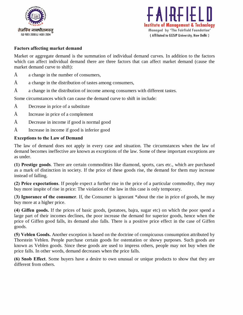
Type of price effects

Thus, a price effect is positive in case of normal goods. There is inverse relationship between price and quantity demanded. It is negative in case of inferior goods (including Giffen goods) where we find direct relationship between price and quantity demanded. Finally, price effect is zero in case of neutral goods where consumer's quantity demanded is fixed.

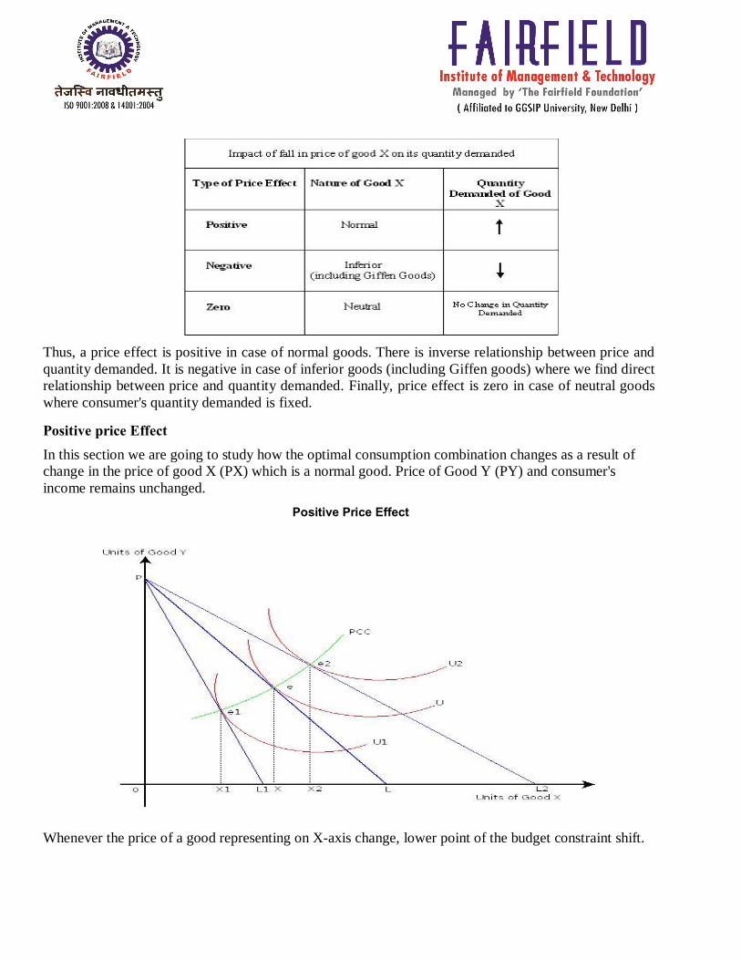
Positive price Effect In this section we are going to study how the optimal consumption combination changes as a result of change in the price of good X (PX) which is a normal good. Price of Good Y (PY) and consumer's income remains unchanged.

Positive Price Effect

Whenever the price of a good representing on X-axis change, lower point of the budget constraint shift.

When the price of good X increases, the budget constraint then becomes steeper, as the lower end point moves leftward. This is shown by budget constraint PL1. The optimal consumption is located at point e1 at which the consumer buys OX1 units of good X. Consumer’s total utility decreases as the optimal consumption combination is located on a lower indifference curve U1.

Similarly, when the price of good X decreases, the budget constraint becomes flatter, as the lower end point moves rightward. This is shown by budget constraint PL2. The optimal consumption is now located at point e2, at which the consumer buys OX2 units of good X. Consumer’s total utility increases as the optimal consumption combination is now located on a higher indifference curve U2.

The curve obtained by joining optimal consumption combinations such as e1, e and e2 is called the price consumption curve (PCC). The PCC in Figure.1 is rising upwards to the right. It shows that the consumer successively moves on a higher indifference curve and becomes better off, with a fall in the price of good X (PX).

NEGATIVE PRICE EFECT

We now study negative price effect. Good X is an inferior good. You will now understand how consumer's optimal consumption combination changes as a result of change in the price of good X (PX) which is an inferior good. Price of good Y (PY) and consumer's income remaining unchanged

When the price of good X decreases, the budget constraint becomes flatter, as the lower end point moves rightward. This is shown by budget constraint PL1. The optimal consumption is now located at point e1, at which the consumer now buys OX1 units of good X. Understand that consumer’s total utility has increased as the optimal consumption point is now located on a higher indifference curve U1. The consumer is better-off in terms of total utility. However, she/he reduces consumption of good X to OX1 units as good X is inferior.

The pcc obtained by joining optimal consumption combinations such as e, and e1, in Figure.2 rises upwards but bending backwards. It shows that the consumer successively moves on a higher indifference curve and becomes better off, with a fall in the price of good X (PX). She/he is also reducing purchase of good X as it is an inferior good.

ZERO EFFECT We now study zero price effect. Good X is a neutral good. You can now see how consumer's optimal consumption combination changes as a result of change in the price of good X (PX) which is a neutral

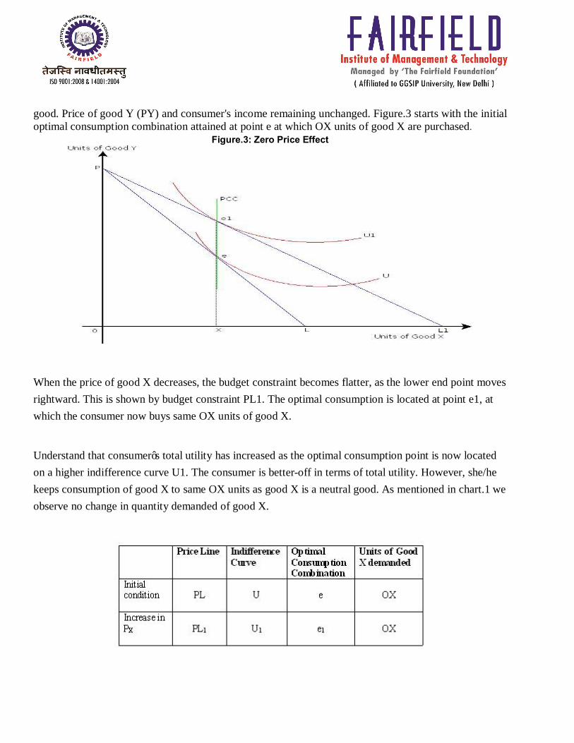
good. Price of good Y (PY) and consumer's income remaining unchanged. Figure.3 starts with the initial optimal consumption combination attained at point e at which OX units of good X are purchased.

Figure.3: Zero Price Effect

When the price of good X decreases, the budget constraint becomes flatter, as the lower end point moves rightward. This is shown by budget constraint PL1. The optimal consumption is located at point e1, at which the consumer now buys same OX units of good X.

Understand that consumer’s total utility has increased as the optimal consumption point is now located on a higher indifference curve U1. The consumer is better-off in terms of total utility. However, she/he keeps consumption of good X to same OX units as good X is a neutral good. As mentioned in chart.1 we observe no change in quantity demanded of good X.

The PCC obtained by joining optimal consumption combinations such as e, and e1, in Figure.3 is a vertical straight line. It shows that the consumer successively moves on a higher indifference curve and becomes better off, with a fall in the price of good X (PX). She/he is keeping purchase of good X fixed as it is a neutral good.

Indifference Curve Analysis - Income Effect Income effect: Meaning - Where there is a change in the income of the consumer, but the prices of the commodities remain constant, there will be a change in consumption made by the consumer. This change in consumption is called the Income Effect.

Equilibrium: Under the income effect there will be a change in the equilibrium position of the consumer and that can be shown in the following diagram.

In the diagram AB is the original price line. T1 is the original equilibrium position. As there is increase in income the new price line or the budget line is CD. T2 is the new equilibrium position. When there is further increase in income, EF becomes the new budget or price line. T3 becomes the new equilibrium position. If we now join T1, T2 and T3, it forms a curve known as income-consumption curve(ICC). The ICC shows the new equilibrium position of the consumer, where there is a change in income, with prices remaining constant.

Types of Income Effect: There are two types of income effect.

1. Positive income effect: When with the increase in income, there is increase in consumption, that is known as Positive Income Effect. 2.Negative Income Effect: when with the increase in income there is decrease in consumption, that is known as Negative Income Effect. The negative income effect is applicable in case of inferior goods. Inferior goods are those goods, which are purchased less as one's income rises.

When the consumer purchases less of commodity X as a result of increase in income, X is the inferior commodity. When the consumer purchases less of commodity Y, as a result of increase in income, Y is the inferior commodity.

Indifference Curve Analysis - Substitution Effect Meaning: When there is a change in the price of one commodity, and when the price of another

commodity remains unchanged or constant, the income of the consumer must be changed in such a way that the consumer is neither better off nor worse off. He remains at the same old position. Under that circumstance, if there is a change in the consumption, that would be due to the Substitution Effect. Equilibrium: We can find out the equilibrium position of the consumer in the following diagram.

In the above diagram AB is the original price or budget line. T is the original equilibrium position. There is a fall in the price of X. So the new budget line is AC. To put the consumer at the same old position we draw another budget or price line DE, which will meet the indifference curve at the point T1. So the movement from T to T1 on the indifference curve IC shows the substitution effect. Here the consumer substitutes n->n1 of Y to get m->m1 more of X because the price of X is now comparatively cheaper than the price of Y.

UNIT-2 Individual Demand Market Demand

The consumer equilibrium condition determines the quantity of each good the individual consumer will demand. As the example above illustrates, the individual consumer's demand for a particular good—call it good X—will satisfy the law of demand and can therefore be depicted by a downward‐sloping individual demand curve. The individual consumer, however, is only one of many participants in the market for good X. The market demand curve for good X includes the quantities of good X demanded by all participants in the market for good X. The market demand curve is found by taking the horizontal summation of all individual demand curves. For example, suppose that there were just two consumers in the market for good X, Consumer 1 and Consumer 2. These two consumers have different individual demand curves corresponding to their different preferences for good X. The two individual demand curves are depicted in Figure , along with the market demand curve for good X.

Individual Demand Market Demand The consumer equilibrium condition determines the quantity of each good the individual consumer will demand. As the example above illustrates, the individual consumer's demand for a particular good—call it good X—will satisfy the law of demand and can therefore be depicted by a downward‐sloping individual demand curve. The individual consumer, however, is only one of many participants in the market for good X. The market demand curve for good X includes the quantities of good X demanded by all participants in the market for good X. The market demand curve is found by taking the horizontal summation of all individual demand curves. For example, suppose that there were just two consumers in the market for good X, Consumer 1 and Consumer 2. These two consumers have different individual demand curves corresponding to their different preferences for good X. The two individual demand curves are depicted in Figure , along with the market demand curve for good X.

Movement along a demand curve There is movement along a demand curve when a change in price causes the quantity demanded to change. It is important to distinguish between movement along a demand curve, and a shift in a demand curve. Movements along a demand curve happen only when the price of the good changes.

If there is a change in price, there is a movement along the demand curve. An increase in price, P1 to P2 causes a change in quantity demand from Q2 to Q1 A change in price doesn’t shift the demand curve – we merely move from one point of demand curve to another.

Shift of a demand curve The shift of a demand curve takes place when there is a change in any non-price determinant of demand, resulting in a new demand curve. When income increases, the demand curve for normal goods shifts outward as more will be demanded at all prices, while the demand curve for inferior goods shifts inward due to the increased attainability of superior substitutes. With respect to related goods, when the price of a good (e.g. a hamburger) rises, the demand curve for substitute goods (e.g. chicken) shifts out, while the demand curve for complementary goods (e.g. tomato sauce) shifts in (i.e. there is more demand for substitute goods as they become more attractive in terms of value for money, while demand for complementary goods contracts in response to the contraction of quantity demanded of the underlying good). An example of a demand curve shifting. The shift from D1 To D2 means an increase in demand with consequences for the other variables

Difference between movement on demand curve and shift of demand curve

Movement on Demand curve Shift of demand curve

1. Movement is caused only by change in own price of the commodity

a) This is caused by change in determinants, other than own price of the commodity

2. Increase or decrease in own price of the commodity is the only cause.

b) There can be several causes: change in income, change in price of substitute goods, change in price of complimentary goods, change in taste and preferences, etc.

3. Movement on demand curve is of two types:

i. Contraction ii. Extension.

c) Shift of demand curve in two ways

i. Decrease in demand curve ii. Increase in demand curve

d) In movement demand curve moves upward or downward on same curve.

4. In shifting demand curve shifts to the right or left from its origin.

ELASTICITY OF DEMAND Price elasticity of demand (PED or Ed) is a measure used in economics to show the responsiveness, or elasticity, of the quantity demanded of a good or service to a change in its price. More precisely, it gives the percentage change in quantity demanded in response to a one percent change in price. It was devised by Alfred Marshall.

It is a measure of responsiveness of the quantity of a good or service demanded to changes in its price.

Measurement of Elasticity of Demand Elasticity of demand is known as price-elasticity of demand. Because elasticity of demand is the degree of change in amount demanded of a commodity in response to a change in price. Price elasticity of demand can be measured through three popular methods. These methods are:

1. Percentage method or Arithmetic method 2. Total Expenditure method

3. Graphic method or point method. 1. Percentage method:-

According to this method price elasticity is estimated by dividing the percentage change in amount demanded by the percentage change in price of the commodity. Thus given the percentage change of both amount demanded and price we can derive elasticity of demand. If the percentage charge in amount demanded is greater than the percentage change in price, the coefficient thus derived will be greater than one. If percentage change in amount demanded is less than percentage change in price, the elasticity is said to be less than one. But if percentage change of both amount demanded and price is same, elasticity of demand is said to be unit.

2. Total expenditure method Total expenditure method was formulated by Alfred Marshall. The elasticity of demand can be measured on the basis of change in total expenditure in response to a change in price. It is worth noting that unlike percentage method a precise mathematical coefficient cannot be determined to know the elasticity of demand. By the help of total expenditure method we can know whether the price elasticity is equal to one, greater than one, less than one. In such a method the initial expenditure before the change in price and the expenditure after the fall in price are compared. By such comparison, if it is found that the expenditure remains the same, elasticity of demand is One (ed=I).

If the total expenditure increases the elasticity of demand is greater than one (ed>l). If the total expenditure diminished with the change in price elasticity of demand is less than one (ed<I). The total expenditure method is illustrated by the following diagram.

3. Graphic method: Graphic method is otherwise known as point method or Geometric method. This method was popularized by method. According to this method elasticity of demand is measured on different points on a straight line demand curve. The price elasticity of demand at a point on a straight line is equal to the lower segment of the demand curve divided by upper segment of the demand curve.

Thus at mid point on a straight-line demand curve, elasticity will be equal to unity; at higher points on the same demand curve, but to the left of the mid-point, elasticity will be greater than unity, at lower points on the demand curve, but to the right of the mid¬point, elasticity will be less than unity.

Factors Affecting Elasticity of Demand Elasticity of demand differs from commodity to commodity. Not only that, elasticity of de¬mand of the same commodity may be different for different persons. These differences in elasticity of demand are due to various causes, which are discussed below: 1. Price level: Generally, the demand for very costly and very cheap goods is elastic. Very costly

goods are demanded by the rich people and hence their demand is not affected much by changes in prices.

For example, increase in the price of Maruti Car from Rs. 3, 00,000 to Rs. 3, 20,000 will not make any noticeable difference in its demand. Similarly, the changes in the price of very cheap goods (such as salt) will not have any effect on their demand, for a very small part of income is spent on such commodities.

2. Availability of Substitutes: The demand for a commodity will be very elastic if some other commodities can be used for it. A small rise in the price of such a commodity will induce consumers to use its substitutes. For example gas, kerosene oil, coal etc. will be used more as fuel if the price of wood increases. On the other hand, the demand of such commodities is inelastic which have no substitutes such as salt.

3. Time period: Longer is the time period more elastic is the demand. In the short period if price of a commodity like petrol is increased, its demand will not fall immediately and hence it would be inelastic or less elastic. But if period is longer alternative sources of energy can be developed and hence demand would be elastic.

4. Proportion of total expenditure spent on the product: If a small proportion of total expenditure is spent on a commodity, its demand will be inelastic such as demand for salt. On the other hand, if a major portion of total expenditure is spent on a commodity, its demand will be more or highly elastic such as demand for luxuries.

5. Habits: Some products which are not essential for some individuals are essential for others. If individuals are habituated of some commodities the demand for such commodities will be usually inelastic, because they will use them even when their prices go up. A smoker generally does not smoke less when the price of cigarette goes up.

6. Nature of the commodities: Generally, the demand for necessaries is inelastic and that for comforts and luxuries of life elastic. This is so because certain goods which are essential to life will be demanded at any price, whereas goods meant for luxuries and comforts can be dispensed with easily if they appear to be costly.

7. Various uses: Generally, a commodity which has several uses will have an elastic demand such as milk, wood etc. On the other hand, a commodity having only one use will have inelastic demand.

8. Postponement: Usually the demand for such commodities whose use can be postponed for some time is elastic. For example, the demand for V.C.R. is elastic because its use can be postponed for some time if its price goes up, but the demand for rice and wheat is inelastic because their use cannot be postponed when their prices increase.

Cross Elasticity of Demand

An economic concept that measures the responsiveness in the quantity demanded of one good when a change in price takes place in another good. The measure is calculated by taking the percentage change in the quantity demanded of one good, divided by the percentage change in price of the substitute good: Cross elasticity of demand is synonymous to "cross price elasticity of demand".

Income Elasticity of Demand A measure of the relationship between a change in the quantity demanded for a particular good and a change in real income. Income elasticity of demand is an economics term that refers to the sensitivity of the quantity demanded for a certain product in response to a change in consumer incomes. The formula for calculating income elasticity of demand is:

Income Elasticity of Demand = % change in quantity demanded / % change in income For example, if the quantity demanded for a good increases for 15% in response to a 10%increase in income, the income elasticity of demand would be 15% / 10% = 1.5. The degree to which the quantity demanded for good changes in response to a change in income depends on whether the good is a necessity or a luxury.

Advertising elasticity of demand

Advertising elasticity of demand (or simply advertising elasticity, often shortened to AED) is an elasticity measuring the effect of an increase or decrease in advertising on a market. Although traditionally considered as being positively related, demand for the good that is subject of the advertising campaign can be inversely related to the amount spent if the advertising is negative.

Definition Good advertising will result in a positive shift in demand for a good. AED is used to measure the effectiveness of this strategy in increasing demand versus its cost. Mathematically, then, AED measures the percentage change in the quantity of a good demanded induced by a given percentage change in spending on advertising in that sector:

SUPPLY Economists describe supply as the relationship between the quantity of a good or service consumers will offer for sale and the price charged for that good. More precisely and formally supply can be thought of as "the total quantity of a good or service that is available for purchase at a given price." Supply Schedules: A supply schedule is a table which lists the possible prices for a good and service and the associated quantity supplied.

The supply schedule gives the relationship between the quantity of a good that producers desire to sell and that good's price, all else held constant

Supply Curve: The supply curve is a graphical representation of the supply schedule with price on the y-axis and quantity on the x-axis.

LAW OF SUPPLY

A microeconomic law stating that, all other factors being equal, as the price of a good or service increases, the quantity of goods or services offered by suppliers increases and vice versa.

The law of supply is a fundamental principle of economic theory which states that, all else equal, an increase in price results in an increase in quantity supplied. In other words, there is a direct relationship between price and quantity: quantities respond in the same direction as price changes. This means that producers are willing to offer more products for sale on the market at higher prices by increasing production as a way of increasing profits. DETERMINANTS OF SUPPLY When price changes, quantity supplied will also change. That is a movement along the same supply curve. When factors other than price changes, supply curve will shift. Here are some determinants of the supply curve. 1. Production cost: Since most private companies’ goal is profit maximization. Higher production cost will lower profit, thus hinder supply. Factors affecting production cost are: input prices, wage rate, government regulation and taxes, etc. 2. Technology: Technological improvements help reduce production cost and increase profit, thus stimulate higher supply. 3. Number of sellers: More sellers in the market increase the market supply. 4. Expectation for future prices: If producers expect future price to be higher, they will try to hold on to their inventories and offer the products to the buyers in the future, thus they can capture the higher price. 5. Taxes and Subsidies

Taxes reduces profits, therefore increase in taxes reduce supply whereas decrease in taxes increase supply. Subsidies reduce the burden of production costs on suppliers, thus increasing the profits. Therefore increase in subsidies increase supply and decrease in subsidies decrease supply. Equilibrium Supply Curve When supply and demand are equal (i.e. when the supply function and demand function intersect) the economy is said to be at equilibrium. At this point, the allocation of goods is at its most efficient because the amount of goods being supplied is exactly the same as the amount of goods being demanded. Thus, everyone (individuals, firms, or countries) is satisfied with the current economic condition. At the given price, suppliers are selling all the goods that they have produced and consumers are getting all the goods that they are demanding.

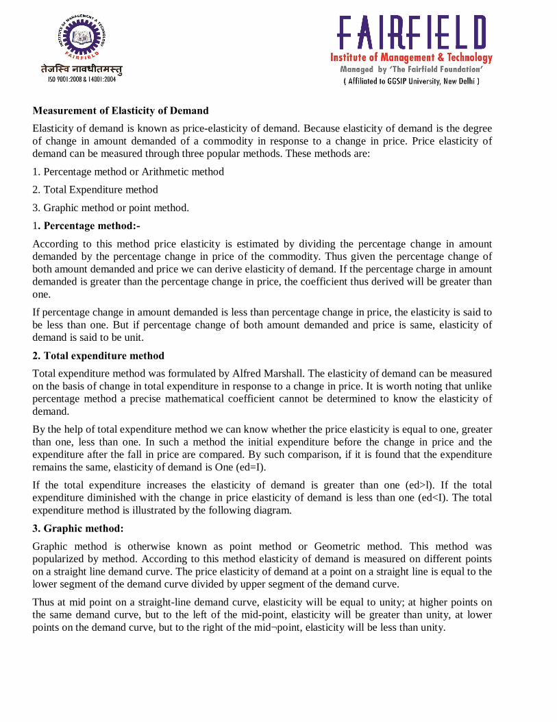
As you can see on the chart, equilibrium occurs at the intersection of the demand and supply curve, which indicates no allocative inefficiency. At this point, the price of the goods will be P* and the quantity will be Q*. These figures are referred to as equilibrium price and quantity. Disequilibrium Disequilibrium occurs whenever the price or quantity is not equal to P* or Q*. 1. Excess Supply If the price is set too high, excess supply will be created within the economy and there will be allocative inefficiency.

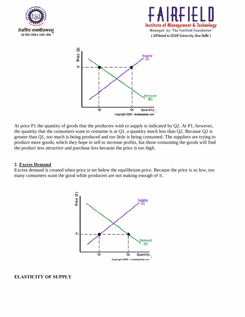
At price P1 the quantity of goods that the producers wish to supply is indicated by Q2. At P1, however, the quantity that the consumers want to consume is at Q1, a quantity much less than Q2. Because Q2 is greater than Q1, too much is being produced and too little is being consumed. The suppliers are trying to produce more goods, which they hope to sell to increase profits, but those consuming the goods will find the product less attractive and purchase less because the price is too high. 2. Excess Demand Excess demand is created when price is set below the equilibrium price. Because the price is so low, too many consumers want the good while producers are not making enough of it.

ELASTICITY OF SUPPLY

Price elasticity of supply (PES or Es) is a measure used in economics to show the responsiveness, or elasticity, of the quantity supplied of a good or service to a change in its price or cost.

The elasticity is represented in numerical form, and is defined as the percentage change in the quantity supplied divided by the percentage change in price.

When the coefficient is less than one, the said good can be described as inelastic; when the coefficient is greater than one, the supply can be described as elastic. An elasticity of zero indicates that quantity supplied does not respond to a price change: it is "fixed" in supply. Such goods often have no labor component or are not produced, limiting the short run prospects of expansion. If the coefficient is exactly one, the good is said to be unitary elastic. The quantity of goods supplied can, in the short term, be different from the amount produced, as manufacturers will have stocks which they can build up or run down.

When supply is perfectly inelastic, a shift in the demand curve has no effect on the equilibrium quantity supplied onto the market. Examples include the supply of tickets for sports or musical venues, and the short run supply of agricultural products (where the yield is fixed at harvest time) the elasticity of supply = zero when the supply curve is vertical.

When supply is perfectly elastic a firm can supply any amount at the same price. This occurs when the firm can supply at a constant cost per unit and has no capacity limits to its production. A change in demand alters the equilibrium quantity but not the market clearing price.

When supply is relatively inelastic a change in demand affects the price more than the quantity supplied. The reverse is the case when supply is relatively elastic. A change in demand can be met without a change in market price.

Determinants

1. Availability of raw materials: For example, availability may cap the amount of gold that can be produced in a country regardless of price. Likewise, the price of Van Gogh paintings is unlikely to affect their supply.

2. Length and complexity of production: Much depends on the complexity of the production process. Textile production is relatively simple. The labor is largely unskilled and production facilities are little more than buildings – no special structures are needed. Thus the PES for textiles is elastic. On the other hand, the PES for specific types of motor vehicles is relatively inelastic. Auto manufacture is a multi-stage process that requires specialized equipment, skilled labor, a large suppliers network and large R&D costs.

3. Mobility of factors: If the factors of production are easily available and if a producer producing one good can switch their resources and put it towards the creation of a product in demand, then it can be said that the PES is relatively elastic. The inverse applies to this, to make it relatively inelastic.

4. Time to respond: The more time a producer has to respond to price changes the more elastic the supply. Supply is normally more elastic in the long run than in the short run for produced goods, since it is generally assumed that in the long run all factors of production can be utilised to increase supply, whereas in the short run only labor can be increased, and even then, changes may be prohibitively costly. For example, a cotton farmer cannot immediately (i.e. in the short run) respond to an increase in the price of soybeans because of the time it would take to procure the necessary land.

5. Excess capacity: A producer who has unused capacity can (and will) quickly respond to price changes in his market assuming that variable factors are readily available.

6. Inventories: A producer who has a supply of goods or available storage capacity can quickly increase supply to market.

Various research methods are used to calculate price elasticity in real life, including analysis of historic sales data, both public and private, and use of present-day surveys of customers' preferences to build up test markets capable of modeling elasticity such changes. Alternatively, conjoint analysis (a ranking of users' preferences which can then be statistically analyzed) may be used. Shifts vs. Movement

For economics, the "movements" and "shifts" in relation to the supply and demand curves represent very different market phenomena: 1. Movements A movement refers to a change along a curve. On the demand curve, a movement denotes a change in both price and quantity demanded from one point to another on the curve. The movement implies that the demand relationship remains consistent. Therefore, a movement along the demand curve will occur when the price of the good changes and the quantity demanded changes in accordance to the original demand relationship. In other words, a movement occurs when a change in the quantity demanded is caused only by a change in price, and vice versa.

Like a movement along the demand curve, a movement along the supply curve means that the supply relationship remains consistent. Therefore, a movement along the supply curve will occur when the price of the good changes and the quantity supplied changes in accordance to the original supply relationship. In other words, a movement occurs when a change in quantity supplied is caused only by a change in price, and vice versa.

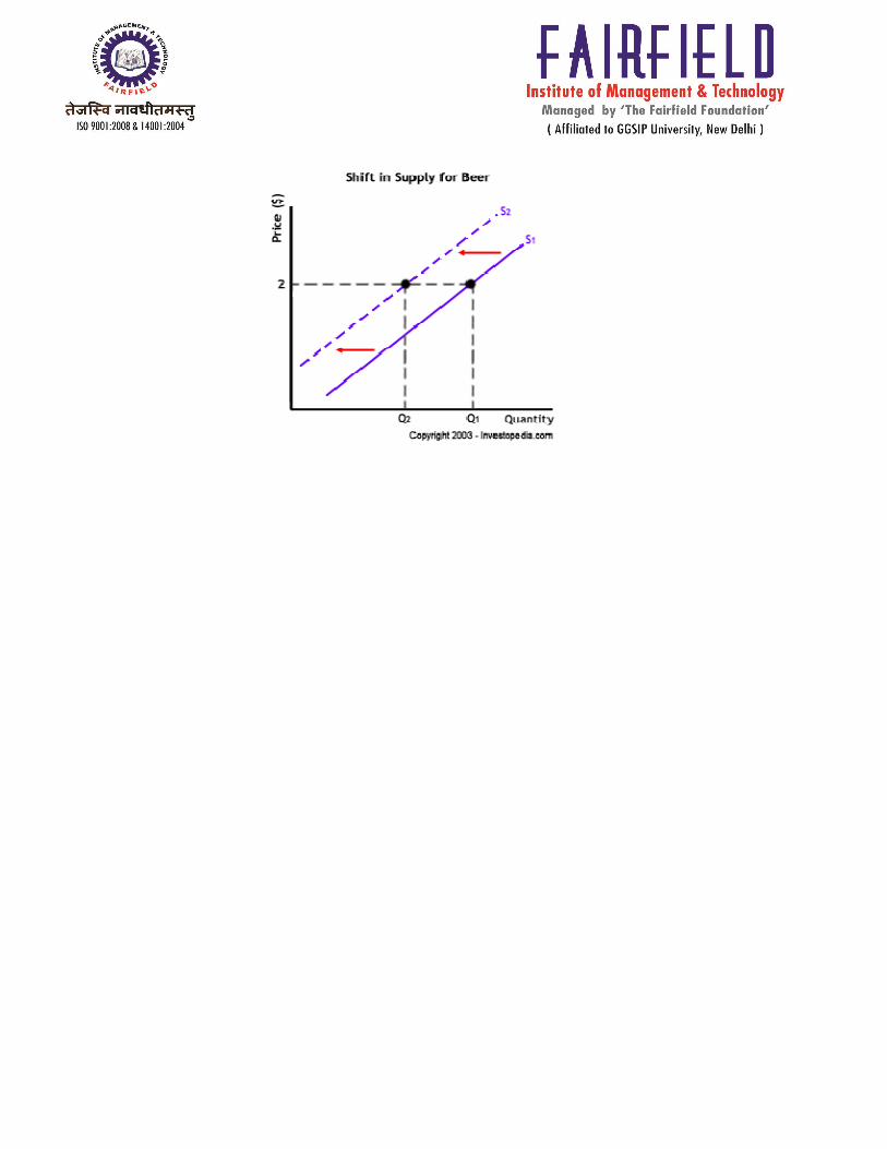
2. Shifts A shift in a demand or supply curve occurs when a good's quantity demanded or supplied changes even though price remains the same. For instance, if the price for a bottle of beer was $2 and the quantity of beer demanded increased from Q1 to Q2, then there would be a shift in the demand for beer. Shifts in the demand curve imply that the original demand relationship has changed, meaning that quantity demand is affected by a factor other than price. A shift in the demand relationship would occur if, for instance, beer suddenly became the only type of alcohol available for consumption.

Conversely, if the price for a bottle of beer was $2 and the quantity supplied decreased from Q1 to Q2, then there would be a shift in the supply of beer. Like a shift in the demand curve, a shift in the supply curve implies that the original supply curve has changed, meaning that the quantity supplied is effected by a factor other than price. A shift in the supply curve would occur if, for instance, a natural disaster caused a mass shortage of hops; beer manufacturers would be forced to supply less beer for the same price.

UNIT-3 Production Production is transformation of tangible inputs (raw materials, semi-finished goods, subassemblies) and intangible inputs (ideas, information, knowledge) into output(goods or services) in a specific period of time at given state of technology. Resources are used in this process to create an output that is suitable for use or has exchange value.

Production Function

Production is transformation of tangible inputs (raw materials, semi-finished goods, subassemblies) and intangible inputs (ideas, information, knowledge) into output(goods or services) in a specific period of time at given state of technology. Output is thus, a function of inputs. Technical relation between inputs and outputs is depicted by production function. It denotes effective combination of inputs.

In economics, a production function relates physical output of a production process to physical inputs or factors of production. In macroeconomics, aggregate production functions are estimated to create a framework in which to distinguish how much of economic growth to attribute to changes in factor allocation (e.g. the accumulation of capital) and how much to attribute to advancing technology. Some non-mainstream economists, however, reject the very concept of an aggregate production function.

Factor of production In economics, factors of production are the inputs to the production process. Finished goods are the output. Input determines the quantity of output i.e. output depends upon input. Input is the starting point and output is the end point of production process and such input-output relationship is called a production function. The product of one industry may be used in another industry. For E.G., wheat is a output for a framer; but when it is used to produce bread it becomes a factor of production. There are three basic (AKA classical) factors of production:

• Land • Labor • Capital • entrepreneur

All three of these are required in combination at a time to produce a commodity. 'Factors of production' may also refer specifically to the 'primary factors', which are stocks including land, labor (the ability to work), and capital goods applied to production. Materials and energy are considered secondary factors in classical economics because they are obtained from land, labor and capital. The primary factors facilitate production but neither become part of the product (as with raw materials) nor become significantly transformed by the production process (as with fuel used to power machinery).

Four factors of production

Concept of production functions The inputs to the production function are commonly termed factors of production and may represent primary factors, which are stocks. Classically, the primary factors of production were Land, Labor and Capital. Primary factors do not become part of the output product, nor are the primary factors, themselves, transformed in the production process.

Production function differs from firm to firm, industry to industry. Any change in the state of technology or managerial ability disturbs the original production function. Production function can be represented by schedules, graph, tables, mathematical equations, TP, AP & MP Curves, isoquant and so on.

Specifying the production function A production function can be expressed in a functional form as the right side of

Q = f (K, L, I, O) Where:

Q = quantity of output K, L, I, O stand for quantities of factors of production (capital, labour, land or organization respectively) used in production

The Law of variable proportions

“ As the proportion of one factor in a combination of factors is increased, after a point, first the marginal and then the average production of that factor will diminish”.

Assumptions of the Law: (i) The state of technology is assumed be given and unchanged. (ii)The law specially operates in the short run because some factors are fixed and the proportion between factors is disturbed. (iii)Variable factor units are homogeneous or identical in amount and quality.

(Iv) The law is based on the possibility of varying the proportions in which the various factors can be combined to produce a product.

Explanation of the law:

The law can be explained with help of a table. The behaviour of output as a result of change in the proportion of variable factors to the fixed factor can be studied through three stages. The table given below explains the short run production function of a firm with some factors variable.

Any change of variable factor to the fixed factor changes the output. The changes due to change in Win in the factors on the total product, average. Product and the marginal product are shown in the table. As the number of laborers increases from 1 to 2, marginal as well as the average product increases. But with the further addition of labour units the average product falls and the marginal falls more speedily.

Average and marginal product continue to fall as more men are put to work. The 7th labour unit adds nothing to total production. After the 7th unit of labour, the eighth labour causes the total product to diminish. In other words the marginal productivity of 8th labour is negative.

Illustration of the Law: The law of variable proportion is illustrated in the following table and figure. Suppose there is a given amount of land in which more and more labour (variable factor) is used to produce wheat.

Units of Labour Total Product Marginal Product Average Product

1 2 2 2

2 6 4 3

3 12 6 4

4 16 4 4

5 18 2 3.6

6 18 0 3

7 14 -4 2

8 8 -6 1

Diagrammatic Representation

Measures quantity of variable factors. Y-axis measures output. In the diagram quantity of the variable factor is increased. Total product rises at first, remains constant at point N, and then starts falling. Average product and marginal product curves are represented by AP and MP. AP and MP curve also rise and decline. MP curve starts declining earlier than the AP curve. The behaviour of these total, average and marginal products of the variable factor as a result of the increase in its amount is generally divided into three stages.

Stage-I (Increasing Return)

Total product increases at an increasing rate to the point F. corresponding to the point F marginal product increases up to this level. From the point F total product goes on rising at a diminishing rate and marginal product starts falling -but is still higher than average product and the AP continues to rise. 1st stage ends where MP curve cuts AP curve from above.

Stage-II (Diminishing Return)

The second stage begins from the point of intersection of AP and MP curves and ends at that point where" MP is zero. At this stage both MP and AP go on falling and both of them are positive. The total product goes

on rising at a diminishing rate. This stage is known as the stage of diminishing return. This is stage where a firm wishes to operate.

Stage-Ill (Negative Return)

In the third stage marginal product of variable factor is zero. MP curve cuts the OX-axis at point M. In this stage the total product starts diminishing. Total product continues to decline. As MP is negative this stage is also known as the stage of negative return.

Total, average, and marginal product

Total Product Curve

Average and marginal product curve

The total product (or total physical product) of a variable factor of production identifies what outputs are possible using various levels of the variable input. This can be displayed in either a chart that lists the output level corresponding to various levels of input, or a graph that summarizes the data into a “total product curve”. The diagram shows a typical total product curve. In this example, output increases as more inputs are employed up until point A. The maximum output possible with this production process is Qm. (If there are other inputs used in the process, they are assumed to be fixed.) The average physical product is the total production divided by the number of units of variable input employed. It is the output of each unit of input. If there are 10 employees working on a production

process that manufactures 50 units per day, then the average product of variable labour input is 5 units per day.

The average product typically varies as more of the input is employed, so this relationship can also be expressed as a chart or as a graph. A typical average physical product curve is shown (APP). It can be obtained by drawing a vector from the origin to various points on the total product curve and plotting the slopes of these vectors.

The marginal physical product of a variable input is the change in total output due to a one unit change in the variable input (called the discrete marginal product) or alternatively the rate of change in total output due to an infinitesimally small change in the variable input (called the continuous marginal product). The discrete marginal product of capital is the additional output resulting from the use of an additional unit of capital (assuming all other factors are fixed). The continuous marginal product of a variable input can be calculated as the derivative of quantity produced with respect to variable input employed. The marginal physical product curve is shown (MPP). It can be obtained from the slope of the total product curve. Because the marginal product drives changes in the average product, we know that when the average physical product is falling, the marginal physical product must be less than the average. Likewise, when the average physical product is rising, it must be due to a marginal physical product greater than the average. For this reason, the marginal physical product curve must intersect the maximum point on the average physical product curve.

Notes: MPP keeps increasing until it reaches its maximum. Up until this point every additional unit has been adding more value to the total product than the previous one. From this point onwards, every additional unit adds less to the total product compared to the previous one – MPP is decreasing. But the average product is still increasing till MPP touches APP. At this point, an additional unit is adding the same value as the average product. From this point onwards, APP starts to reduce because every additional unit is adding less to APP than the average product. But the total product is still increasing because every additional unit is still contributing positively. Therefore, during this period, both, the average as well as marginal products, are decreasing, but the total product is still increasing. Finally we reach a point when MPP crosses the x-axis. At this point every additional unit starts to diminish the product of previous units, possibly by getting into their way. Therefore the total product starts to decrease at this point. This is point A on the total product curve.

Isoquant

An isoquant is one of the ways of presenting production, where the two factors of production are explicitly shown. It represents all possible input combination of two factors, which are capable of producing the same level of output. While an indifference curve mapping helps to solve the utility-maximizing problem of consumers, the isoquant mapping deals with the cost-minimization problem of producers. As producer will be indifferent between such combinations, so it is often referred to as producer’s indifference curve. A family of isoquants can be represented by an isoquant map, a graph combining a number of isoquants, each representing a different quantity of output. Isoquants are also called equal product curves.

Production Isoquant/Isocost Curve

An isoquant shows the extent to which the firm in question has the ability to substitute between the two different inputs at will in order to produce the same level of output. An isoquant map can also indicate decreasing or increasing returns to scale based on increasing or decreasing distances between the isoquant pairs of fixed output increment, as output increases. Isoquant curve analysis helps a producer to find a combination of two factors, which gives him maximum output at minimum cost.

As with indifference curves, two isoquants can never cross. Also, every possible combination of inputs is on an isoquant. Finally, any combination of inputs above or to the right of an isoquant results in more output than any point on the isoquant. Although the marginal product of an input decreases as you increase the quantity of the input while holding all other inputs constant, the marginal product is never negative in the empirically observed range since a rational firm would

Isoquant Map

The isoquant curve

a. The isoquant curve contains all combinations of 2 inputs that produce the same total output. b. All points on an isoquant curve are technically efficient. c. The curve is bowed toward the origin because of the law of diminishing marginal productivity.

d. The slope of the isoquant is called the "Marginal Rate of Technical Substitution" (MRTS) or the

"Marginal Rate of Substitution (MRS). e. For every possible combination of inputs, there is an isoquant. The whole set of isoquants is called

the "isoquant map". The "isoquant map" is a picture of the state of technology. f. It slopes downward from left to right g. Isoquants never touch, intersect each other

Long Run Production - Returns to Scale

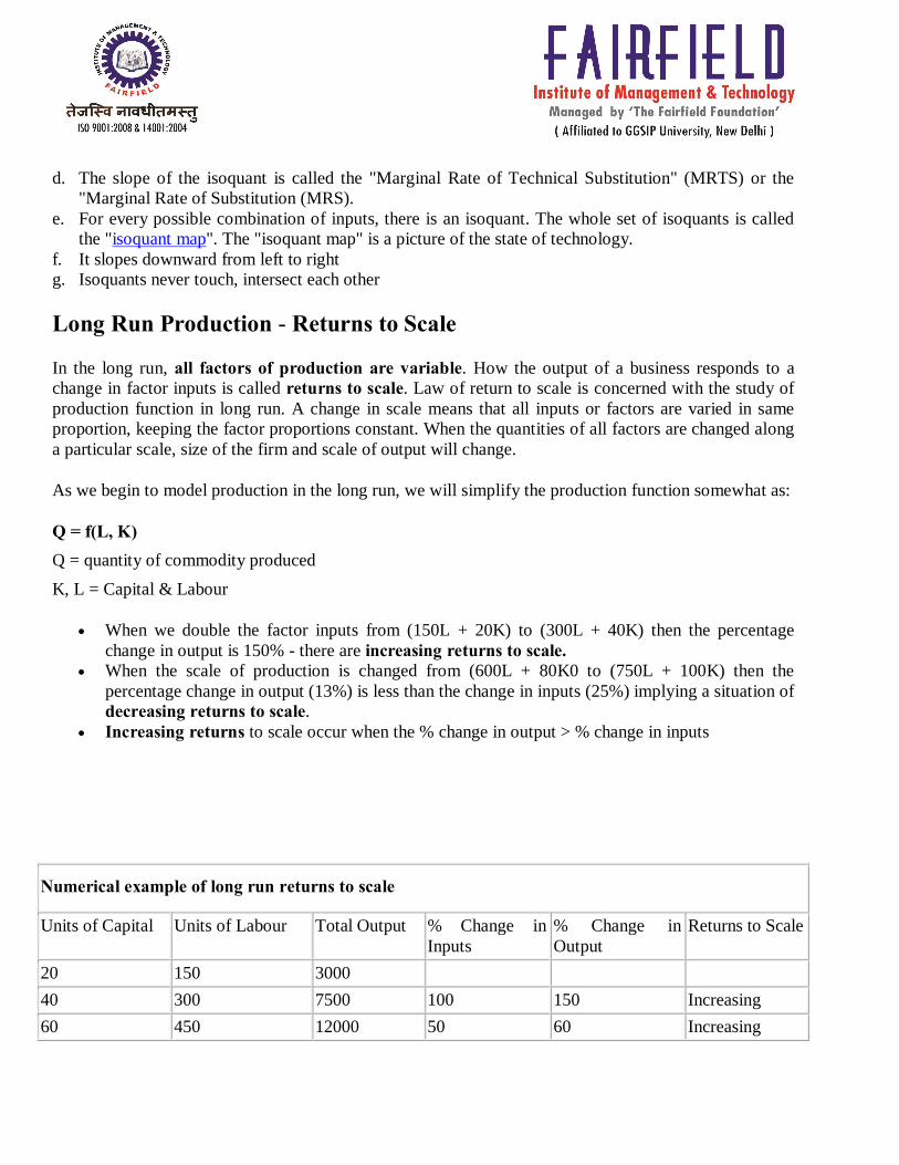
In the long run, all factors of production are variable. How the output of a business responds to a change in factor inputs is called returns to scale. Law of return to scale is concerned with the study of production function in long run. A change in scale means that all inputs or factors are varied in same proportion, keeping the factor proportions constant. When the quantities of all factors are changed along a particular scale, size of the firm and scale of output will change.

As we begin to model production in the long run, we will simplify the production function somewhat as:

Q = f(L, K) Q = quantity of commodity produced K, L = Capital & Labour

• When we double the factor inputs from (150L + 20K) to (300L + 40K) then the percentage change in output is 150% - there are increasing returns to scale.

• When the scale of production is changed from (600L + 80K0 to (750L + 100K) then the percentage change in output (13%) is less than the change in inputs (25%) implying a situation of decreasing returns to scale.

• Increasing returns to scale occur when the % change in output > % change in inputs

Numerical example of long run returns to scale

Units of Capital Units of Labour Total Output % Change in Inputs

% Change in Output

Returns to Scale

20 150 3000 40 300 7500 100 150 Increasing 60 450 12000 50 60 Increasing

• Decreasing returns to scale occur when the % change in output < % change in inputs • Constant returns to scale occur when the % change in output = % change in inputs

The nature of the returns to scale affects the shape of a business’s long run average cost curve. Possible Cases in Long Run Period of Production

The long run period of production usually analyzes the economies of scale which studies the increasing returns to scale or economies of mass production. It tends to provided information about the unit cost and the size of operation in the production of goods. The economies of scale primarily directed to reduce the unit costs from the increasing size of the operation. That is why the larger firms are more economically viable in the long run production as it diminishes the production cost. Take note that the economies of scale tends to increase in specialization and division of labor. This may lead to increase production inputs and expands the production output.

1. Decreasing Returns to Scale (Increasing Cost): When the firm becomes large it is likely to encounter problem in the production of a particular product because of the increase average cost of operation. This is the problem of management when increase of production input by 60% the production output reaches only to 40%. In this notion the production is less cheap at a certain scale when it is already large in scale. It requires large-scale machinery or division of labor to produce greater production output. Hence, the Decreasing Returns to scale occur when the percent change in output is greater in percent for the change in inputs.

2. Constant Returns to Scale (Constant Cost): There is a time for a firm to enjoy a long range of production output for which the average cost is the same proportion to both production input and output. If there is an increase of the number of machines by 50% then there is also an increase of the number of units produced by 50%. This is a constant returns in machinery production. Hence, the Constant Returns to scale occur when the average cost do not increase as a result of diseconomies of scale.

80 600 16000 33 33 Constant 100 750 18000 25 13 Decreasing

3. Increasing Return to Scale (Decreasing Cost): This is known as the economies of scale wherein the firm’s increase in all production inputs and outputs. Supposing a firm increases the inputs by 50% the return of scale increases to 60%.The economies scale expands productive capacity in the long run as it operated by machines and other sophisticated technology that may reduce the overhead cost in producing the products. This is more on capital-intensive production wherein there are more equipment utilize than workers in the production process. In the long run, the manufacturing sectors with high capital investment of equipment results to higher production output that expands the profitability of the firms. The economies of scale are the reduction of unit cost in the long run of operation. The expansion of the firm through a mass production provides greater units of output.

Difference between return to factor & return to scale

The difference between returns to a variable factor and returns to scale flow from the Law of Diminishing Returns and must be understood in the parameters of the concepts of short-run and long-run.

Short run (return to factor) is a period when production can be increased only with increase in variable factors because fixed factors are constant; the firms cannot change their sizes and scales in the short run. When output is increased by more quantities of variable factors with the fixed factor held constant, the the proportion between the fixed and variable factors changes and the change in output follows the Law of Variable Proportions in terms of which initially the total rises at a higher rate, then it become constant because marginal product reaches zero and eventually it falls. This locus of the marginal product (MP) i.e. incremental output is called the Law of Variable Proportions.

Long run (return to scale) is defined as a period which allows the firm to change their sizes and scales to increase output i.e. in the long run all factors are variable but even in this case initially there are increasing returns to scale i.e. the total output rises with fast speed, then it becomes constant and eventually the total output falls because marginal product (MP) becomes negative. This situation is subservient to the Law of Diminishing Returns to Scale.

The basic difference between the laws of returns to a variable factor and the laws of returns to scale lies in the assumptions on which these laws are based.

1. In case of the laws of returns to a variable factor, only one input is variable—all other inputs remaining constant—whereas in case of the laws of returns to scale, all the inputs are variable.

2. The law of returns to a variable factor is a short run phenomenon because supply of capital in the short run is inelastic. On the contrary, the laws of returns to scale are a long run phenomenon because supply of all the inputs in the long run is elastic and more and more of all the inputs can be employed. In the analysis of the input–output relationship, therefore, in case of the law of returns to a variable factor a single-variable production function is used whereas in case of the laws of returns to scale a two-variable production function is used.

UNIT-4 Concept of cost The term ‘cost’ means the amount of expenses [actual or national] incurred on or attributable to specified thing or activity. A producer requires various factors of production or inputs for producing commodity. He pays them in a form of money. Such money expenses incurred by a firm in the production of a commodity are called cost of production.

As per Institute of cost and work accounts (ICWA) India, Cost is ‘measurement in monetary terms of the amount of resources used for the purpose of production of goods or rendering services. To get the results we make efforts. Efforts constitute cost of getting the results. It can be expressed in terms of money; it means the amount of expenses incurred on or attributable to some specific thing or activity.

Short run cost & long run cost

Short-run cost

Short run cost varies with output, when unlike long run cost all the factors are not variable. This cost becomes relevant, when a firm has to decide whether or not to produce more in the immediate future. This cost can be divided into two components of fixed and variable cost on the basis of variability of factors of production.

1. Fixed cost: In the short period the expenses incurred on fixed factors are called the fixed cost. These costs don’t change with changes in level of output. “The fixed cost is those cost that don’t vary with the size of output.”

2. Variable cost: VC are those costs which are incurred on the use of variable factors of production. They directly change with production. The rate of increase of total variable cost is determined by the law of returns.

3. Total cost: TC of a firm for various levels of output are the sum of total fixed cost and total

variable cost.

4. Average cost: per unit cost of a good is called its average cost. Average cost is total cost divided by output.

AC= TC/Q AC= AFC+AVC

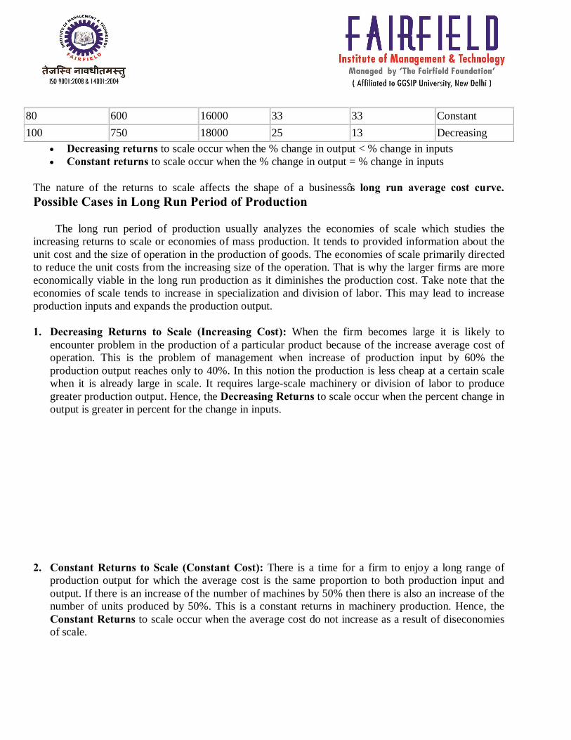
a) Average fixed cost: AFC is total fixed cost /total output. AFC is the per unit cost of the fixed factor of production.

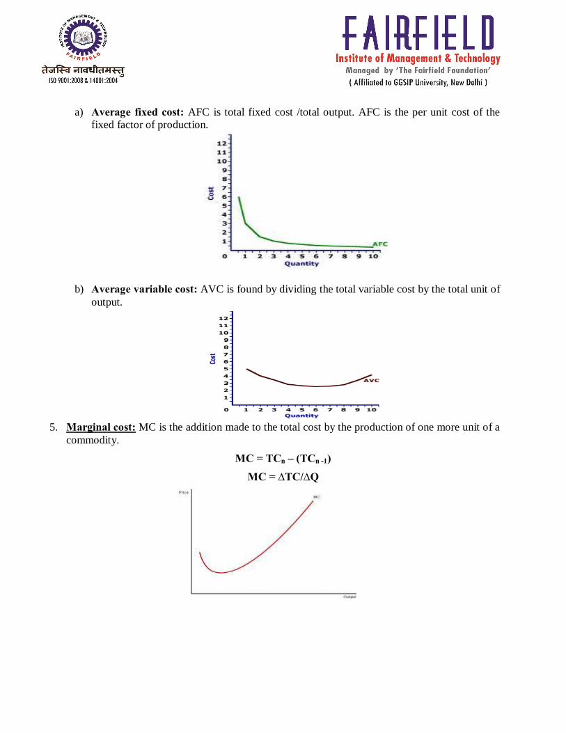
b) Average variable cost: AVC is found by dividing the total variable cost by the total unit of output.

5. Marginal cost: MC is the addition made to the total cost by the production of one more unit of a

commodity.

MC = TCn – (TCn -1)

MC = ∆TC/∆Q

Long-run cost In the long run, all factors of production are variable. Hence there is no distinction between fixed and variable cost. All cost are variable cost and there is nothing like fixed cost.

a) Long run average cost b) Long run marginal cost

a) Long run avg. cost: LRAC refers to minimum possible per unit cost of producing different

quantities of output of a good in the long period.

b) Long run marginal cost: change in the total cost in the long run, due to the production of one more unit, is called LRMC.

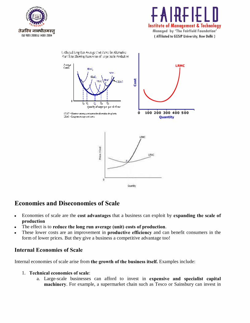
Economies and Diseconomies of Scale

• Economies of scale are the cost advantages that a business can exploit by expanding the scale of production

• The effect is to reduce the long run average (unit) costs of production. • These lower costs are an improvement in productive efficiency and can benefit consumers in the

form of lower prices. But they give a business a competitive advantage too!

Internal Economies of Scale

Internal economies of scale arise from the growth of the business itself. Examples include:

1. Technical economies of scale: a. Large-scale businesses can afford to invest in expensive and specialist capital

machinery. For example, a supermarket chain such as Tesco or Sainsbury can invest in

technology that improves stock control. It might not, however, be viable or cost-efficient for a small corner shop to buy this technology.

b. Specialization of the workforce: Larger businesses split complex production processes into separate tasks to boost productivity. The division of labour in mass production of motor vehicles and in manufacturing electronic products is an example.

c. The law of increased dimensions. This is linked to the cubic law where doubling the height and width of a tanker or building leads to a more than proportionate increase in the cubic capacity – this is an important scale economy in distribution and transport industries and also in travel and leisure sectors.

2. Marketing economies of scale and monopsony power: A large firm can spread its advertising and marketing budget over a large output and it can purchase its inputs in bulk at negotiated discounted prices if it has monopsony (buying) power in the market. A good example would be the ability of the electricity generators to negotiate lower prices when negotiating coal and gas supply contracts. The big food retailers have monopsony power when purchasing supplies from farmers.

3. Managerial economies of scale: This is a form of division of labour. Large-scale manufacturers employ specialists to supervise production systems and oversee human resources.

4. Financial economies of scale: Larger firms are usually rated by the financial markets to be more ‘credit worthy’ and have access to credit facilities, with favorable rates of borrowing. In contrast, smaller firms often face higher rates of interest on overdrafts and loans. Businesses quoted on the stock market can normally raise fresh money (i.e. extra financial capital) more cheaply through the issue of equities. They are also likely to pay a lower rate of interest on new company bonds issued through the capital markets.

5. Network economies of scale: This is a demand-side economy of scale. Some networks and services have huge potential for economies of scale. That is, as they are more widely used they become more valuable to the business that provides them. The classic examples are the expansion of a common language and a common currency. We can identify networks economies in areas such as online auctions, air transport networks. Network economies are best explained by saying that the marginal cost of adding one more user to the network is close to zero, but the resulting benefits may be huge because each new user to the network can then interact, trade with all of the existing members or parts of the network. The expansion of e-commerce is a great example of network economies of scale – how many of you are devotees of the EBay web site or Facebook?

External economies of scale

• External economies of scale occur within an industry and from the expansion of it • Examples include the development of research and development facilities in local universities

that several businesses in an area can benefit from and spending by a local authority on improving the transport network for a local town or city.

• Likewise, the relocation of component suppliers and other support businesses close to the main centre of manufacturing are also an external cost saving.

Diseconomies of scale

A firm may eventually experience a rise in average costs caused by diseconomies of scale.

Diseconomies of scale a firm might be caused by:

1. Control – monitoring the productivity and the quality of output from thousands of employees in big corporations is imperfect and costly.

2. Co-operation - workers in large firms may feel a sense of alienation and subsequent loss of morale. If they do not consider themselves to be an integral part of the business, their productivity may fall leading to wastage of factor inputs and higher costs. A fall in productivity means that workers may be less productively efficient in larger firms.

3. Loss of control over costs – big businesses may lose control over fixed costs such as expensive head offices, management expenses and marketing costs. There is also a risk that very expensive capital projects involving new technology may prove ineffective and leave the business with too much under-utilized capital.

Evaluation: Do economies of scale always improve the welfare of consumers?

• Standardization of products: Mass production might lead to a standardization of products – limiting the amount of consumer choice.

• Lack of market demand: Market demand may be insufficient for economies of scale to be fully exploited leaving businesses with a lot of spare capacity.

• Developing monopoly power: Businesses may use economies of scale to build up monopoly power and this might lead to higher prices, a reduction in consumer welfare and a loss of allocative efficiency.

• Protecting monopoly power: Economies of scale might be used as a barrier to entry – whereby existing firms can drive prices down if there is a threat of the entry of new suppliers.

Explicit Cost and Implicit Cost

Explicit cost:

All those expenses that a firm incurs to make payment to others are called explicit cost. An explicit cost is a direct payment made to others in the course of running a business, such as wage, rent and materials. Explicit costs are taken into account along with implicit ones when considering economic profit. Accounting profit only takes explicit costs into account.

Implicit cost:

Implicit cost is the cost of entrepreneur’s own factors or resources. These includes the rewards for the entrepreneurs self owned land, building, labour & capital. In economics, an implicit cost, also called an imputed cost, implied cost.

Implicit costs also represent the divergence between economic profit (total revenues minus total costs, where total costs are the sum of implicit and explicit costs) and accounting profit (total revenues minus only explicit costs). Since economic profit includes these extra opportunity costs, it will always be less than or equal to accounting profit.

Private and Social Cost

Private cost refers to the cost of production incurred & provided for by an individual firm engaged in the production of a commodity. It is found out to get private profits. It includes both explicit as well as implicit cost. A firm is interested in minimizing private cost.

Social cost refers to the cost of producing a commodity to the society as a whole. It takes into consideration of all those costs which were borne by the society directly or indirectly. It is a sum of private cost & external cost. for example, from pollution of the atmosphere.

SOCIAL COST = PRIVATE COST + EXTERNALITY

For example: - a chemical factory emits wastage as a by-product into nearby rivers and into the atmosphere. This creates negative externalities which impose higher social costs on other firms and consumers. e.g. clean up costs and health costs.

Another example of higher social costs comes from the problems caused by traffic congestion in towns, cities and on major roads and motor ways. It is important to note though that the manufacture, purchase and use of private cars can also generate external benefits to society. This why cost-benefit analysis can be useful in measuring and putting some monetary value on both the social costs and benefits of production.

Key Concepts:

Private Costs + External Costs = Social Costs

If external costs > 0, then private costs < social costs.

Then society tends to:

• Price the good or service too low and Produces or consumes too much of the good or service. Different Costs Matter:

Private costs for a producer of a good, service, or activity include the costs the firm pays to purchase capital equipment, hire labor, and buy materials or other inputs. While this is straightforward from the business side, it also is important to look at this issue from the consumers’ perspective. Field, in his 1997 text, Environmental Economics provides an example of the private costs a consumer faces when driving a car:

The private costs of this (driving a car) include the fuel and oil, maintenance, depreciation, and even the drive time experienced by the operator of the car.

Private costs are paid by the firm or consumer and must be included in production and consumption decisions. In a competitive market, considering only the private costs will lead to a socially efficient rate of output only if there are no external costs.

External costs, on the other hand, are not reflected on firms’ income statements or in consumers’ decisions. However, external costs remain costs to society, regardless of who pays for them. Consider a firm that attempts to save money by not installing water pollution control equipment. Because of the firm’s actions, cities located down river will have to pay to clean the water before it is fit for drinking, the public may find that recreational use of the river is restricted, and the fishing industry may be harmed. When external costs like these exist, they must be added to private costs to determine social costs and to ensure that a socially efficient rate of output is generated.

Social costs include both the private costs and any other external costs to society arising from the production or consumption of a good or service. Social costs will differ from private costs, for example, if a producer can avoid the cost of air pollution control equipment allowing the firm’s production to imposes costs (health or environmental degradation) on other parties that are adversely affected by the air pollution. Remember too, it is not just producers that may impose external costs on society. Let’s also view how consumers’ actions also may have external costs using Field’s previous example on driving:2

The social costs include all these private costs (fuel, oil, maintenance, insurance, depreciation, and operator’s driving time) and also the cost experienced by people other than the operator who are exposed to the congestion and air pollution resulting from the use of the car.

The key point is that even if a firm or individual avoids paying for the external costs arising from their actions, the costs to society as a whole (congestion, pollution, environmental cleanup, visual degradation, wildlife impacts, etc.) remain. Those external costs must be included in the social costs to ensure that society operates at a socially efficient rate of output.

REVENUE

Meaning of Revenue: The amount of money that a producer receives in exchange for the sale proceeds is known as revenue. For example, if a firm gets Rs. 16,000 from sale of 100 chairs, then the amount of Rs. 16,000 is known as revenue. Revenue refers to the amount received by a firm from the sale of a given quantity of a commodity in the market.

Revenue is a very important concept in economic analysis. It is directly influenced by sales level, i.e., as sales increases, revenue also increases.

Concept of Revenue: The concept of revenue consists of three important terms; Total Revenue, Average Revenue and Marginal Revenue.

Total Revenue (TR): Total Revenue refers to total receipts from the sale of a given quantity of a commodity. It is the total income of a firm. Total revenue is obtained by multiplying the quantity of the commodity sold with the price of the commodity. Total Revenue = Quantity × Price

For example, if a firm sells 10 chairs at a price of Rs. 160 per chair, then the total revenue will be: 10 Chairs × Rs. 160 = Rs 1,600

Average Revenue (AR): Average revenue refers to revenue per unit of output sold. It is obtained by dividing the total revenue by the number of units sold.

Average Revenue = Total Revenue/Quantity For example, if total revenue from the sale of 10 chairs @ Rs. 160 per chair is Rs. 1,600, then:

Average Revenue = Total Revenue/Quantity = 1,600/10 = Rs 160

AR and Price are the Same: We know, AR is equal to per unit sale receipts and price is always per unit. Since sellers receive revenue according to price, price and AR are one and the same thing. This can be explained as under:

TR = Quantity × Price … (1)

AR = TR/Quantity …… (2) Putting the value of TR from equation (1) in equation (2), we get

AR = Quantity × Price / Quantity

AR = Price

AR Curve and Demand Curve are the Same: A buyer’s demand curve graphically represents the quantities demanded by a buyer at various prices. In other words, it shows the various levels of average revenue at which different quantities of the good are sold by the seller. Therefore, in economics, it is customary to refer AR curve as the Demand Curve of a firm.

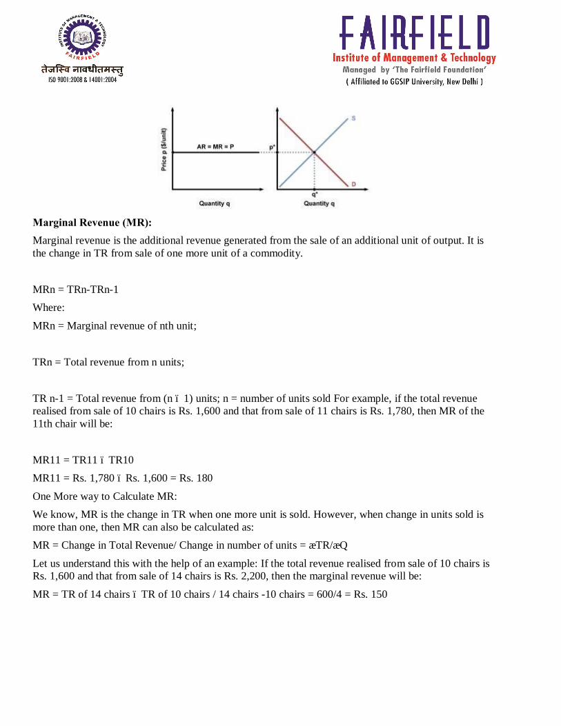
Marginal Revenue (MR): Marginal revenue is the additional revenue generated from the sale of an additional unit of output. It is the change in TR from sale of one more unit of a commodity.

MRn = TRn-TRn-1 Where:

MRn = Marginal revenue of nth unit;

TRn = Total revenue from n units;

TR n-1 = Total revenue from (n – 1) units; n = number of units sold For example, if the total revenue realised from sale of 10 chairs is Rs. 1,600 and that from sale of 11 chairs is Rs. 1,780, then MR of the 11th chair will be:

MR11 = TR11 – TR10 MR11 = Rs. 1,780 – Rs. 1,600 = Rs. 180

One More way to Calculate MR: We know, MR is the change in TR when one more unit is sold. However, when change in units sold is more than one, then MR can also be calculated as: MR = Change in Total Revenue/ Change in number of units = ∆TR/∆Q

Let us understand this with the help of an example: If the total revenue realised from sale of 10 chairs is Rs. 1,600 and that from sale of 14 chairs is Rs. 2,200, then the marginal revenue will be:

MR = TR of 14 chairs – TR of 10 chairs / 14 chairs -10 chairs = 600/4 = Rs. 150

TR is summation of MR: Total Revenue can also be calculated as the sum of marginal revenues of all the units sold.

It means, TRn = MR1 + M2 + MR3 + ……….MRn

or, TR = ∑MR