B.C. SPRINKLER IRRIGATION MANUAL - British …...B.C. SPRINKLER IRRIGATION MANUAL Chapter 4 Editor...

BB..CC.. SSPPRRIINNKKLLEERR IIRRRRIIGGAATTIIOONN MMAANNUUAALL

Chapter 4

Editor

Ted W. van der Gulik, P.Eng. Senior Engineer

Authors

Stephanie Tam, P.Eng. Water Management Engineer

Andrew Petersen, P.Ag.

Regional Resource Specialist

Prepared and Web Published by

Ministry of Agriculture

2014 ISSUE

LIMITATION OF LIABILITY AND USER’S RESPONSIBILITY

The primary purpose of this manual is to provide irrigation professionals and consultants with a methodology to properly design an agricultural irrigation system. This manual is also used as the reference material for the Irrigation Industry Association’s agriculture sprinkler irrigation certification program. While every effort has been made to ensure the accuracy and completeness of these materials, additional materials may be required to complete more advanced design for some systems. Advice of appropriate professionals and experts may assist in completing designs that are not adequately convered in this manual. All information in this publication and related materials are provided entirely “as is” and no representations, warranties or conditions, either expressed or implied, are made in connection with your use of, or reliance upon, this information. This information is provided to you as the user entirely at your risk. The British Columbia Ministry of Agriculture and the Irrigation Industry Association of British Columbia, their Directors, agents, employees, or contractors will not be liable for any claims, damages or losses of any kind whatsoever arising out of the use of or reliance upon this information.

Chapter 4 Crop, Soil and Climate 33

4 CROP, SOIL AND CLIMATE Designing an efficient irrigation system requires a good understanding of soil texture, soil moisture and crop relationships. The effects of soil type, crop rooting depth, and climate are important when considering irrigation system application rates and set times. Six specific design criteria need to be selected or calculated: 1). Maximum Soil Water Deficit, 2). Maximum Irrigation System Application Rate, 3). Maximum Irrigation Interval, 4). Peak Evapotranspiration Rate, 5). Peak Irrigation System Flow Rate and 6). Annual Irrigation System Demand.

4.1 Maximum Soil Water Deficit The maximum soil water deficit is the maximum amount of water that can be removed by the crop from the soil before irrigation is required. Maximum soil water deficit is measured in inches or millimeters. It is calculated by determining crop rooting depths, the soil's available water storage capacity and the crop's availability coefficient.

Equation 4.1 Soil Water Storage (SWS)

AWSCRDSWS ×=

where SWS = soil water storage (in or mm) RD = rooting depth (ft or m) AWSC = available water storage capacity (in/ft or mm/m) Equation 4.2 Maximum Soil Water Deficit (MSWD)

ACSWSMSWD ×= where MSWD = maximum soil water deficit (in or mm)

SWS = soil water storage (in or mm) AC = availability coefficient (decimal)

34 B.C. Sprinkler Irrigation Manual

Effective Rooting Depth (RD)

The effective rooting depth (RD) of a mature crop is that depth of soil from which a crop removes a significant amount of water. The normal effective rooting depths for crops grown in deep, uniformly porous, friable and fertile soils are given in Table 4.1. These depths must be modified for soils which do not permit normal root development. Compaction of the surface soil, excessively coarse subsoil, impervious subsoil, poor soil drainage, high water tables, soil chemistry and fertility problems may inhibit normal root development and reduce the effective rooting depth for irrigation. Irrigation systems must be designed for mature crop requirements. More frequent irrigations at shorter durations will be required for crops that have not reached full rooting depth.

Available Water Storage Capacity (AWSC)

The available water storage capacity (AWSC) of the soil is the depth of water that can be retained between field capacity and the permanent wilting point. The capacity of a soil to store water depends upon the composition of the soil by particle size (texture) and the soil particle arrangement (structure). To obtain an estimate of the water holding capacity of a soil it is necessary to determine soil textures within the effective rooting depth of the crop to be irrigated.

The textural characteristics of mineral soils are distinguished by the percent composition of sand, silt and clay, as shown in Figure 4.1. If the soil texture is not known, soil samples should be taken and analyzed. Refer to Soil Sampling factsheet. Table 4.2 can be used to estimate the AWSC of the soil once texture has been determined. The total AWSC of the effective rooting zone is obtained by adding the AWSC of the various textural layers. Soil Sampling (Factsheet 611.100-1)

Availability Coefficient (AC)

The availability coefficient (AC) is used to determine the amount of water that the crop can extract from the soil. Different crops have varying availability coefficients. Only a portion of the total AWSC is readily available for plant use. The availability coefficient (AC) is the maximum fraction of the total AWSC stored in the root zone that can be removed by the crop before irrigation is required. Allowing depletion of soil moisture to exceed the levels indicated by the availability coefficient may result in crop stress and a reduction in crop yields. Table 4.3 lists the availability coefficient for various crop types.


Figure 4.1 Soil Texture Triangle

Table 4.1 Effective Rooting Depth of Mature Crops Shallow

0.45 m (1.5 ft) Medium Shallow

0.6 m (2 ft) Medium Deep 0.9 m (3 ft)

Deep 1.2 m (4 ft)

Cabbages Cauliflowers Cucumbers Lettuce Onions Pasture species Radishes Turnips

Beans Beets Blueberries Broccoli Carrots Celery Peas Potatoes Spinach Strawberries Tomatoes Tree Fruits (3’ x 10’)

Brussels Sprouts Cereal Clover (red) Corn (sweet) Eggplant Kiwifruit Peppers Squash Saskatoons Tree Fruits (6’ x 12’)

Alfalfa Asparagus Blackberries Corn (field) Grapes Loganberries Raspberries Sugar beets Tree Fruits (12’ x 18’)


Table 4.2 Available Water Storage Capacity (AWSC)

Soil Texture

AWSC

Inches of Water per Foot of Soil (in/ft)

Millimetre of Water per Metre of Soil (mm/m)

Sand (S) 1.0 83

Loamy Sand (LS) 1.2 100

Sandy Loam (SL) 1.5 125

Fine Sandy Loam (Fine SL) 1.7 142

Loam (L) 2.1 167

Silt (Si) 2.0 167

Silty Loam (SiL) 2.5 192

Silty Clay (SiC) 2.5 208

Clay Loam (CL) 2.4 192

Silty Clay Loam (SiCL) 2.4 200

Clay (CL) 2.4 200

Heavy Clay (Heavy C) 2.5 208

Organic Soils (muck) 3.0 250

Table 4.3 Crop Availability Coefficients Crop Maximum Percent

[% expressed as decimal]

Peas 0.35

Potatoes 0.35

Tree Fruits 0.40

Grapes 0.40

Tomatoes 0.40

Others 0.50


Example 4.1 Maximum Soil Water Deficit in Armstrong

Question: A farmer near Armstrong intends to grow alfalfa on a deep sandy loam soil. What is the

Maximum Soil Water Deficit (MSWD)? Information: Crop type alfalfa 1 Effective rooting depth (RD) (Table 4.1) 4.0 ft 2 ft or m Availability coefficient (AC) (Table 4.3) 0.50 3 Soil Depth

[ft] or [m] Soil

Texture RD

[ft] or [m] AWSC [in/ft] or [mm/m]

(Table 4.2) SWS

[in] or [mm]

0 – 1 ft Sandy Loam 1 ft 4 x 1.5 in/ft 5 = 1.5 in 6 1 – 2 ft Sandy Loam 1 ft 4 x 1.5 in/ft 5 = 1.5 in 6 2 – 3 ft Sandy Loam 1 ft 4 x 1.5 in/ft 5 = 1.5 in 6 3 – 4 ft Sandy Loam 1 ft 4 x 1.5 in/ft 5 = 1.5 in 6 Calculation: Determine Total Soil Water Storage (SWS). Step 1. Calculate SWS for each soil depth interval that can be reached by the crop’s roots. Use the

first interval as an example. Equation 4.1 SWS = RD x AWSC = 1 4 ft x 1.5 5 in/ft = 1.5 6 in Step 2. Add all SWS for each soil depth interval to obtain Total SWS. Total SWS = SWS(0-1 ft) + SWS(1-2 ft) + SWS(2-3 ft) + SWS(3-4 ft) = ( 1.5 6 + 1.5 6 + 1.5 6 + 1.5 6 ) in = 6.0 7 in Answer: Equation 4.2 MSWD = Total SWS x AC = 6.0 7 ft x 0.50 3 in = 3.0 8 in


Example 4.2 Maximum Soil Water Deficit in Osoyoos

Question: A farmer in Osoyoos is growing apples in a soil that consists of 2 ft of loam, 2 ft of loamy

sand. Calculate the maximum soil water deficit (MSWD). Information: While tree fruits have a rooting depth of 4 ft (Table 4.1), the rooting depth for dwarf tree

fruits is limited to 3 ft.

Crop type Apples 1 Effective rooting depth (RD) (Table 4.1) 3 ft 2 ft or m Availability coefficient (AC) (Table 4.3) 0.40 3 Soil Depth

[ft] or [m] Soil

Texture RD

[ft] or [m] AWSC [in/ft] or [mm/m]

(Table 4.2) SWS

[in] or [mm]

0 – 1 ft Loam 1 ft 4 x 2.1 in/ft 5 = 2.1 in 6 1 – 2 ft Loam 1 ft 4 x 2.1 in/ft 5 = 2.1 in 6 2 – 3 ft Loamy Sand 1 ft 4 x 1.2 in/ft 5 = 1.2 in 6 3 – 4 ft – – 4 x – 5 = – 6 Calculation: Determine Total Soil Water Storage (SWS). Step 1. Calculate SWS for each soil depth interval that can be reached by the crop’s roots. Use the

first interval as an example. Equation 4.1 SWS = RD x AWSC = 1 4 ft x 2 5 in/ft = 2 6 in Step 2. Add all SWS for each soil depth interval to obtain Total SWS. Total SWS = SWS(0-1 ft) + SWS(1-2 ft) + SWS(2-3 ft) + SWS(3-4 ft) = ( 2.1 6 + 2.1 6 + 1.2 6 + – 6 ) in = 5.2 7 in Answer: Equation 4.2 MSWD = Total SWS x AC = 5.2 7 ft x 0.40 3 in = 2.1 8 in


4.2 Maximum Irrigation System Application Rate The rate of water infiltration into the soil surface depends on soil texture, structure and type of ground cover. The irrigation system application rate should not exceed the infiltration capability of the soil. The objective of a good irrigation design is to eliminate runoff and puddling of water on the soil surface. Exceeding the maximum soil infiltration rate shown in Table 4.4 may lead to soil degradation by compaction or soil erosion. Soil compaction and erosion can result in lower crop yields if poor irrigation practices are ongoing from year to year. Proper nozzle selection and maintenance is important to ensure that maximum soil infiltration rates are not exceeded.

Table 4.4 provides estimated maximum soil infiltration rates based on various soil textures and ground cover under normal irrigation practices. The rates shown are for irrigation set times of 4 hours or greater. The maximum soil infiltration rate for irrigation set times less than 4 hours may be higher. The values shown in Table 4.4 are for level ground and should be reduced if the irrigated area is on a slope. A general rule is to reduce the maximum application rate by 25% for field slopes exceeding 10% and 50% for field slopes exceeding 20%. If unsure, field tests under actual sprinkler conditions should be conducted to determine an accurate and safe maximum design application rate.

Table 4.4 Maximum Soil Infiltration Rate

Soil Texture Grass Sod Cultivated

[in/hr] [mm/hr] [in/hr] [mm/hr] Sand (S) 0.75 19.0 0.40 10.0

Loamy Sand (LS) 0.65 16.5 0.35 9.0

Sandy Loam (SL) 0.45 11.5 0.25 6.0

Fine Sandy Loam (Fine SL) 0.40 10.0 0.25 6.0

Loam (L) 0.35 9.0 0.20 5.0

Silt (Si) 0.35 9.0 0.20 5.0

Silty Loam (SiL) 0.35 9.0 0.20 5.0

Silty Clay (SiC) 0.35 9.0 0.20 5.0

Clay Loam (CL) 0.30 7.5 0.15 4.0

Silty Clay Loam (SiCL) 0.30 7.5 0.15 4.0

Clay (CL) 0.25 6.0 0.10 3.0

Heavy Clay (Heavy C) 0.25 6.0 0.10 3.0

Organic Soils (muck) 0.50 12.5 0.50 13.0


4.3 Maximum Irrigation Interval The Maximum Irrigation Interval (Max II) is the maximum number of days between irrigations during peak climatic conditions that a crop can sustain optimum growth and production. It is calculated by dividing the MSWD by the peak evapotranspiration rate. The actual irrigation interval may be less than the maximum irrigation interval if the irrigation system applies less than the total amount of water that can be stored in the soil (MSWD).

The maximum irrigation interval is always calculated during peak conditions. Actual irrigation intervals can exceed the calculated maximum irrigation interval during non peak conditions.

Equation 4.3 Maximum Irrigation Interval

ETPeakMSWDIIMax =

where Max II = maximum irrigation interval (day) MSWD = maximum soil water deficit (in) Peak ET = peak evapotranspiration (in/day) Table 4.5

4.4 Peak Evapotranspiration Rate Evapotranspiration (ET) is a measure of the rate at which water is transpired by plants plus the moisture that is evaporated from the plants and soil surface.

For irrigation system design the Peak ET rate used is actually an average of the Peak ET rates determined for each day over the duration of the maximum irrigation interval during the peak of the season. This is referred to as the Peak ET rate and is provided as a daily value. This averaged Peak ET rate will decrease as the irrigation interval increases (larger MSWD values). The reason the values decrease over larger irrigation intervals is that it is less likely that there will be a succession of very hot days over a longer irrigation interval than there would be over a shorter interval.

Since the MSWD determines how much water can be stored within the crop’s root zone, a larger MSWD will have a longer irrigation interval if the soil profile is completely filled with water. The Peak ET rate will therefore decrease with an increase in MSWD. Table 4.5 provides an estimate of the Peak ET rates for a range of MSWD values. The Peak ET values are given in inches per day or mm per day for MSWD ranging from 25 to 125 mm (i.e. 1 to 5 inches) of water that can be stored in the soil. The Peak ET rates shown in the 1 inch or 25mm column should not generally be used for irrigation system design except in extreme conditions. Climate change may impact this however. See section 4.7.


Table 4.5 Peak Evapotranspiration Rates for Various B.C. Locations

Location Maximum Soil Water Deficit (Depth of Water)

1 in 25 mm

2 in 50 mm 3 in 75 mm 4 in 100 mm 5 in 125 mm in/d mm/d in/d mm/d in/d mm/d in/d mm/d in/d mm/d

100 Mile House 0.26 6.6 0.24 6.1 0.23 5.8 0.22 5.6 0.22 5.6

Abbotsford 0.18 4.6 0.16 4.1 0.15 3.8 0.14 3.6 0.14 3.6

Agassiz 0.18 4.6 0.16 4.1 0.15 3.8 0.14 3.6 0.14 3.6

Alexis Creek 0.18 4.6 0.16 4.1 0.15 3.8 0.14 3.6 0.14 3.6

Armstrong 0.26 6.6 0.23 5.8 0.21 5.3 0.20 5.1 0.19 4.8

Ashcroft 0.36 9.1 0.32 8.1 0.30 7.6 0.29 7.4 0.28 7.1

Aspen Grove 0.27 6.9 0.23 5.8 0.21 5.3 0.20 5.1 0.20 5.1

Barriere 0.24 6.1 0.21 5.3 0.20 5.1 0.19 4.8 0.18 4.6

Baynes Lake 0.28 7.1 0.26 6.6 0.25 6.4 0.24 6.1 0.23 5.8

Campbell River 0.28 7.1 0.22 5.6 0.20 5.1 0.18 4.6 0.17 4.3

Canal Flats 0.30 7.6 0.28 7.1 0.26 6.6 0.25 6.4 0.25 6.4

Castlegar 0.36 9.1 0.33 8.4 0.31 7.9 0.30 7.6 0.29 7.4

Cawston 0.38 9.7 0.34 8.6 0.32 8.1 0.31 7.9 0.30 7.6

Chase 0.24 6.1 0.22 5.6 0.21 5.3 0.20 5.1 0.20 5.1

Cherryville 0.23 5.8 0.22 5.6 0.21 5.3 0.20 5.1 0.20 5.1

Chilliwack 0.21 5.3 0.19 4.8 0.17 4.3 0.16 4.1 0.16 4.1

Clinton 0.26 6.6 0.24 6.1 0.23 5.8 0.22 5.6 0.22 5.6

Cloverdale 0.18 4.6 0.16 4.1 0.14 3.6 0.13 3.3 0.13 3.3

Comox 0.28 7.1 0.22 5.6 0.20 5.1 0.18 4.6 0.16 4.1

Creston 0.20 5.1 0.19 4.8 0.18 4.6 0.18 4.6 0.17 4.3

Dawson Creek 0.21 5.3 0.19 4.8 0.19 4.8 0.18 4.6 0.18 4.6

Donald 0.16 4.1 0.14 3.6 0.14 3.6 0.13 3.3 0.13 3.3

Douglas Lake 0.23 5.8 0.21 5.3 0.21 5.3 0.20 5.1 0.20 5.1

Duncan 0.20 5.1 0.17 4.3 0.16 4.1 0.15 3.8 0.15 3.8

Ellison 0.27 6.9 0.24 6.1 0.23 5.8 0.21 5.3 0.21 5.3

Fort Fraser 0.22 5.6 0.20 5.1 0.19 4.8 0.18 4.6 0.18 4.6

Fort Steele 0.26 6.6 0.23 5.8 0.22 5.6 0.21 5.3 0.20 5.1

Fort St. John 0.21 5.3 0.19 4.8 0.19 4.8 0.18 4.6 0.18 4.6

Golden 0.17 4.3 0.15 3.8 0.15 3.8 0.14 3.6 0.14 3.6

Grand Forks 0.21 5.3 0.19 4.8 0.19 4.8 0.18 4.6 0.18 4.6

Grandview 0.29 7.4 0.27 6.9 0.25 6.4 0.24 6.1 0.24 6.1

Grasmere 0.26 6.6 0.23 5.8 0.22 5.6 0.21 5.3 0.20 5.1

Grindrod 0.19 4.8 0.16 4.1 0.14 3.6 0.14 3.6 0.13 3.3

Hazelton 0.22 5.6 0.19 4.8 0.19 4.8 0.19 4.8 0.19 4.8

Hixon 0.18 4.6 0.16 4.1 0.16 4.1 0.15 3.8 0.15 3.8

Hope 0.28 7.1 0.25 6.4 0.22 5.6 0.21 5.3 0.20 5.1

Invermere 0.27 6.9 0.25 6.4 0.23 5.8 0.22 5.6 0.21 5.3

Joe Rich 0.21 5.3 0.18 4.6 0.16 4.1 0.15 3.8 0.15 3.8

Jura 0.28 7.1 0.24 6.1 0.22 5.6 0.21 5.3 0.20 5.1

Kamloops 0.33 8.4 0.30 7.6 0.28 7.1 0.27 6.9 0.26 6.6


Table 4.5 Peak Evapotranspiration Rates for Various B.C. Locations


1 in 25 mm

2 in 50 mm 3 in 75 mm 4 in 100 mm 5 in 125 mm in/d mm/d in/d mm/d in/d mm/d in/d mm/d in/d mm/d

Kelowna 0.28 7.1 0.25 6.4 0.24 6.1 0.23 5.8 0.22 5.6

Keremeos 0.31 7.9 0.30 7.6 0.29 7.4 0.28 7.1 0.28 7.1

Kersley 0.24 6.1 0.23 5.8 0.22 5.6 0.22 5.6 0.22 5.6

Kettle Valley 0.29 7.4 0.28 7.1 0.27 6.9 0.26 6.6 0.26 6.6

Kimberley 0.34 8.6 0.32 8.1 0.30 7.6 0.28 7.1 0.27 6.9

Ladner 0.16 4.1 0.14 3.6 0.13 3.3 0.13 3.3 0.12 3.0

Langley 0.17 4.3 0.14 3.6 0.14 3.6 0.13 3.3 0.12 3.0

Lillooet 0.33 8.4 0.30 7.6 0.28 7.1 0.27 6.9 0.26 6.6

Lister 0.23 5.8 0.21 5.3 0.21 5.3 0.20 5.1 0.20 5.1

Lumby 0.27 6.9 0.24 6.1 0.23 5.8 0.22 5.6 0.21 5.3

Lytton 0.36 9.1 0.32 8.1 0.30 7.6 0.28 7.1 0.28 7.1

Malakwa 0.23 5.8 0.20 5.1 0.19 4.8 0.19 4.8 0.18 4.6

Merritt 0.30 7.6 0.28 7.1 0.26 6.6 0.25 6.4 0.25 6.4

Nanaimo 0.26 6.6 0.21 5.3 0.19 4.8 0.17 4.3 0.16 4.1

Natal 0.21 5.3 0.19 4.8 0.18 4.6 0.17 4.3 0.17 4.3

Notch Hill 0.24 6.1 0.21 5.3 0.20 5.1 0.19 4.8 0.18 4.6

Oliver 0.29 7.4 0.26 6.6 0.24 6.1 0.23 5.8 0.23 5.8

Osoyoos 0.33 8.4 0.30 7.6 0.28 7.1 0.27 6.9 0.26 6.6

Oyster River 0.14 3.6 0.13 3.3 0.12 3.0 0.11 2.8 0.11 2.8

Parksville 0.21 5.3 0.17 4.3 0.16 4.1 0.15 3.8 0.14 3.6

Pitt Meadows 0.16 4.1 0.14 3.6 0.13 3.3 0.12 3.0 0.12 3.0

Port Alberni 0.28 7.1 0.23 5.8 0.20 5.1 0.19 4.8 0.18 4.6

Prince George 0.18 4.6 0.16 4.1 0.15 3.8 0.15 3.8 0.14 3.6

Princeton 0.28 7.1 0.26 6.6 0.25 6.4 0.23 5.8 0.23 5.8

Quesnel 0.29 7.4 0.27 6.9 0.26 6.6 0.25 6.4 0.25 6.4

Radium 0.23 5.8 0.21 5.3 0.20 5.1 0.19 4.8 0.19 4.8

Riske Creek 0.31 7.9 0.29 7.4 0.28 7.1 0.27 6.9 0.27 6.9

Saanichton 0.19 4.8 0.17 4.3 0.16 4.1 0.15 3.8 0.15 3.8

Salmon Arm 0.19 4.8 0.17 4.3 0.17 4.3 0.16 4.1 0.16 4.1

Smithers 0.18 4.6 0.16 4.1 0.15 3.8 0.14 3.6 0.14 3.6

Spillimacheen 0.23 5.8 0.20 5.1 0.19 4.8 0.18 4.6 0.18 4.6

Sumas 0.20 5.1 0.18 4.6 0.17 4.3 0.16 4.1 0.15 3.8

Summerland 0.30 7.6 0.28 7.1 0.26 6.6 0.24 6.1 0.24 6.1

Terrace 0.32 8.1 0.31 7.9 0.30 7.6 0.29 7.4 0.28 7.1

Vancouver 0.24 6.1 0.20 5.1 0.18 4.6 0.17 4.3 0.16 4.1

Vanderhoof 0.21 5.3 0.20 5.1 0.20 5.1 0.19 4.8 0.19 4.8

Vavenby 0.19 4.8 0.17 4.3 0.16 4.1 0.15 3.8 0.14 3.6

Vernon 0.26 6.6 0.23 5.8 0.22 5.6 0.21 5.3 0.21 5.3

Walhachin 0.31 7.9 0.30 7.6 0.29 7.4 0.28 7.1 0.27 6.9

Westwold 0.30 7.6 0.28 7.1 0.27 6.9 0.26 6.6 0.25 6.4

Williams Lake 0.30 7.6 0.29 7.4 0.28 7.1 0.27 6.9 0.26 6.6 Values in the 1-inch (2.5-cm) column should not be used except for special circumstances. They are shown here for

comparison only.


Example 4.3 Maximum Irrigation Interval in Armstrong

Question: What is the maximum irrigation interval for a farmer in Armstrong with a soil and crop that

have a maximum soil water deficit of 3 inches? Information: Farm location Armstrong 1 Maximum soil water deficit (MSWD) 3 in 2 in or mm Peak evapotranspiration (ET) (Table 4.5) 0.21 3 in/day Answer: Equation 4.2 Max II = MSWD Peak ET

= 3 2 in

0.21 3 in/day = 14 8 days

4.5 Peak Irrigation System Flow Rate Determining a peak irrigation system flow rate is often required to estimate water source capability and to provide a design check on the flow rate used in an irrigation system design. The peak flow rate can also be used for licencing purposes by determining the maximum withdrawal rate allowed from a surface or groundwater source. A peak irrigation system flow rate is determined by combining crop, soils and climate data with an acceptable risk factor. A risk factor is the number of years out of ten that an irrigation system will be deficient in supplying the crop water requirement. A very low risk factor should be used on fruit or vegetable crops as severe crop loss could result from a water shortage. Forage crops, on the other hand, can sustain higher risk values. In this manual a risk factor of 10% is used in determining the peak flow rate for all crops in the tables provided.

Table 4.6 can be used as a guide in determining the peak water supply flow rate for a field using a 10% risk factor and the Peak ET rate. Field shape, soil type, root depth, irrigation system type and farm management may result in a field requiring a higher flow rate in some instances. Irrigation systems designed at flow rates higher than the values per acre indicated in Table 4.6 should be assessed to determine if improvements can be made.

The peak flow rate is provided in gpm/acre or m3/hr/hectare.


Helpful Tips – Peak Flow Rate and Irrigation System Design

The peak flow rate determined in Table 4.6 and 4.7 of this chapter requires that the irrigation system needs to operate 24 hours per day, 7 days a week. In other words, continuously during peak conditions. The values also assume the irrigation system has an efficiency of 72%. Following this design process will ensure that the irrigation system is taking the lowest peak flow rate possible from surface water sources or groundwater. This will help maintain minimum stream flows for fish and reduce groundwater draw down that could affect other users.

Table 4.6 Estimated Peak Irrigation System Flow Rate Requirements (using 10% risk factor)

ET Irrigation System Flow Rates [in/d] [mm/d] [US gpm/acre] [m3/hr/ha] 0.16 4.1 4.0 2.24

0.18 4.6 4.5 2.52

0.20 5.1 5.0 2.80

0.22 5.6 5.5 3.10

0.23 5.8 6.0 3.36

0.25 6.4 6.5 3.64

0.27 6.9 7.0 3.92

0.29 7.4 7.5 4.20

0.31 7.9 8.0 4.48

For irrigation system design, use the following guide to determine a peak flow rate for the irrigation system:

1. If an irrigation water licence indicates a peak flow rate, use the flow rate stated on the licence.

2. If water is supplied by a water purveyor, use the flow rate established by the purveyor (Table 4.8).

3. If neither of the first two options are available and the farm is near one of the locations listed in Table 4.5, the following options can then be used:

Option 1 (recommended)

Follow Example 4.1 or 4.2 to obtain maximum soil water deficits (MSWD)

Use the closest MSWD value available in Table 4.5 to determine a peak ET rate.

Locate the flow rate that corresponds to the peak ET rate in Table 4.6. If the flow rate is between two values in Table 4.6,


choose the lower one. These flow rate estimates are based on a 10% risk factor, meaning the farm may be short of water once in ten years. Note the comments in section 4.7.

Option 1 is recommended since MSWD is taken into account instead of using an average value; therefore, a more accurate peak flow rate may be obtained.

Option 2

Table 4.7 gives quick estimates of peak irrigation flow rates based on ET rates, an average deep-rooted crop in a medium-textured soil with a 3-inch (average) MSWD for various locations in BC.

Table 4.7 Estimated Peak Irrigation Flow Rate Requirements for B.C. Locations1,2

Location Flow Rate [US gpm/acre]3 Location Flow Rate

[US gpm/acre]3 Location Flow Rate [US gpm/acre]3

Abbotsford 4.0 Golden 4.0 Oliver 7.0

Agassiz 4.0 Grand Forks 5.0 100 Mile House 5.5

Alexis Creek 4.0 Grandview Flats 5.5 Osoyoos 8.0

Armstrong 5.0 Grasmere 5.5 Oyster River 4.0

Ashcroft 8.0 Grindrod 4.0 Parksville 4.0

Aspen Grove 5.0 Hazelton 5.0 Pitt Meadows 4.0

Barriere 5.0 Hixon 4.0 Port Alberni 5.0

Baynes Lake 6.5 Hope 5.0 Prince George 4.0

Campbell River 5.0 Invermere 6.0 Princeton 6.0

Canal Flats 6.0 Kamloops 6.5 Quesnel 6.0

Castlegar 8.0 Kelowna 6.0 Radium 5.0

Cawston 8.0 Keremeos 7.5 Riske Creek 7.0

Chase 5.0 Kersley 5.5 Saanichton 4.0

Cherryville 5.0 Kettle Valley 7.0 Salmon Arm 4.5

Chilliwack 4.5 Kimberley 7.0 Smithers 4.0

Clinton 6.0 Ladner 4.0 Spillimacheen 5.0

Cloverdale 4.0 Langley 4.0 Sumas 4.5

Comox 5.0 Lillooet 7.5 Summerland 6.5

Creston 4.5 Lister 5.0 Terrace 5.5

Dawson Creek 4.0 Lumby 5.5 Vancouver 4.5

Douglas Lake 5.0 Lytton 8.0 Vanderhoof 5.0

Duncan 4.0 Malakwa 5.0 Vernon 5.0

Ellison 6.0 Merritt 6.5 Walhachin 6.5

Fort Fraser 5.0 Nanaimo 5.0 Westwold 6.5

Fort Steele 5.5 Natal 4.5 Williams Lake 6.0

Fort St. John 4.0 Notch Hill 5.0 1 Based on peak evapotranspiration rates on an average deep-rooted crop in a medium-textured soil (values in Table

2.1), as well as overall topographic knowledge of each location. 2 Based on 10% risk factor, i.e., water shortage once in 10 years. 3 Multiply values in US gpm/acre by 0.156 to convert to L/s/ha.


Water Purveyor

In the Okanagan Basin and Fraser Valley, irrigation water is often supplied to producers by a water purveyor such as an Irrigation District or a municipality. In these cases, the water purveyor will hold the licensed volume for the withdrawal of water from the source and will also be responsible for the operation and maintenance of the intake works. Water purveyors will usually supply the farm with a peak flow determined by the climate, soil and acreage to be irrigated.

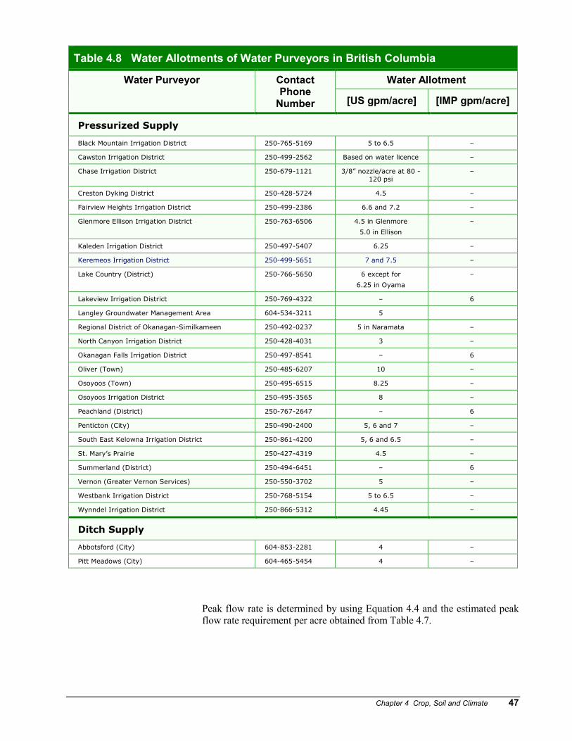
Purveyors may provide pressurized water to the farm gate via the municipal infrastructure or via a ditch system where the farmer is responsible for pumping irrigation water onto the farm. Table 4.8 provides peak flows for a number of water purveyors in British Columbia. For farms located within a water purveyor boundary and receiving irrigation supply from a purveyor, irrigation designs must stay within the peak flow rates established by the water purveyor.

Clarification – Peak Flow Rates Calculated in Manual Examples

The design examples 5.1, 6.2 and 7.1 in the following chapters all use the same farm layout for the wheel move sprinkler, travelling gun and center pivot designs. However the peak flow rates that are determined for each are slightly different. This was done intentionally to show that there are different methods for determining a peak flow rate.

Example 5.1 uses soils and climate information to determine an appropriate irrigation interval which ends up with a flow rate of 693 gpm that is higher than the other two. This methodology does not take into account the10% risk factor as indicated in Table 4.6 using the Peak ET rate to determine peak flow.

Example 6.2 uses the information from Table 4.6 and ends up with a flow rate of 630 gpm. The 10% risk is now applied and therefore the flow rate used is 10% less than example 5.1.

Example 7.1 uses a different formula for determining the peak flow rate for the center pivot system. The pivot without the end gun covers 94 acres. Using the information in Table 4.6 the pivot flow rate would be 494 gpm (5.25 gpm/acre x 94 acres However the formula used for the pivot uses an efficiency value of 80% rather than 72% and the flow rate calculated is therefore less at 466 gpm. If the estimated flow rate of the end gun is added then the total flow rate is 553 gpm. The flow rate for the pivot is less as the system is more efficient and it is not irrigating the entire area as the other two systems do.


Peak flow rate is determined by using Equation 4.4 and the estimated peak flow rate requirement per acre obtained from Table 4.7.

Table 4.8 Water Allotments of Water Purveyors in British Columbia

Water Purveyor Contact Phone

Number

Water Allotment

[US gpm/acre] [IMP gpm/acre]

Pressurized Supply

Black Mountain Irrigation District 250-765-5169 5 to 6.5 –

Cawston Irrigation District 250-499-2562 Based on water licence –

Chase Irrigation District 250-679-1121 3/8” nozzle/acre at 80 - 120 psi

–

Creston Dyking District 250-428-5724 4.5 –

Fairview Heights Irrigation District 250-499-2386 6.6 and 7.2 –

Glenmore Ellison Irrigation District 250-763-6506 4.5 in Glenmore 5.0 in Ellison

–

Kaleden Irrigation District 250-497-5407 6.25 –

Keremeos Irrigation District 250-499-5651 7 and 7.5 –

Lake Country (District) 250-766-5650 6 except for 6.25 in Oyama

–

Lakeview Irrigation District 250-769-4322 – 6

Langley Groundwater Management Area 604-534-3211 5

Regional District of Okanagan-Similkameen 250-492-0237 5 in Naramata –

North Canyon Irrigation District 250-428-4031 3 –

Okanagan Falls Irrigation District 250-497-8541 – 6

Oliver (Town) 250-485-6207 10 –

Osoyoos (Town) 250-495-6515 8.25 –

Osoyoos Irrigation District 250-495-3565 8 –

Peachland (District) 250-767-2647 – 6

Penticton (City) 250-490-2400 5, 6 and 7 –

South East Kelowna Irrigation District 250-861-4200 5, 6 and 6.5 –

St. Mary’s Prairie 250-427-4319 4.5 –

Summerland (District) 250-494-6451 – 6

Vernon (Greater Vernon Services) 250-550-3702 5 –

Westbank Irrigation District 250-768-5154 5 to 6.5 –

Wynndel Irrigation District 250-866-5312 4.45 –

Ditch Supply

Abbotsford (City) 604-853-2281 4 –

Pitt Meadows (City) 604-465-5454 4 –


Equation 4.4 System Peak Flow Rate

AreaIrrigatedAcreperequirementRRateFlowPeakEstimatedRateFlowPeak ×=

where Peak Flow Rate = irrigation system peak flow rate [US gpm] Estimated Peak Flow Rate Requirement per Acre = values from Table 4.7 [US gpm/acre] Irrigated Area = entire area covered by irrigation system [acres]

Example 4.4 System Peak Flow Rate in Armstrong

Question: What is the peak flow rate of a wheelmove irrigation system that irrigates 40 acres of

alfalfa in Armstrong? Information: Farm location Armstrong 1 Estimated peak flow rate requirement per acre (Table 4.7) 5.0 2 US gpm/acre Irrigated area 40 3 acres Answer: Equation 4.4 Peak

Flow Rate = Estimated Peak Flow Rate Requirement per Acre x Irrigated Area = 5.0 2 US gpm/acre x 40 3 acres = 200 4 US gpm

4.6 Annual Irrigation System Demand Annual irrigation system demand is determined to ensure that the irrigation system does not exceed the water use as stated on a water licence or provided by a water purveyor. Water law in B.C. requires all users extracting water from a surface water source to obtain a water licence from the Ministry of Environment before such usage is authorized.

As of the printing date of this manual, withdrawal from ground water does not require licensing in B.C. but is expected to change in the near future. However, an estimate of the peak irrigation system flow rate is helpful in determining the well casing size and also if the groundwater source is capable of supplying the required flow.

In some cases, peak withdrawal rates are also shown on a surface water licence.


Annual Water Requirement

The maximum annual irrigation requirements shown in Table 4.8 are the best estimates for maximum demand crops such as alfalfa and tree fruits for the locations shown. Crops which are not irrigated for an entire season will be proportionately less. Table 4.9 lists the estimated annual crop water requirements based on various MSWD for various BC locations. Irrigation system application efficiencies must be applied to the values in Table 4.9 to determine the annual irrigation water requirements (Equation 4.5).

Equation 4.5 Annual Water Requirement

%100×=EfficiencynApplicatio

equirementRWaterCropAnnualEstimatedequirementRWaterAnnual

where Annual Water Requirement = annual water required by irrigation system [in] Estimated Annual Crop Water Requirement = values from Table 4.9 Application Efficiency = values from Table 3.1

Example 4.5 Annual Water Requirement in Armstrong

Question: What is the annual water requirement of alfalfa irrigated by a wheelmove irrigation system

in Armstrong with MSWD of 2.5 from Example 4.2? Information: Farm location Armstrong 1 MSWD 2.5 in 2 in or mm Estimated annual crop requirement (Table 4.9) 12 in 3 in or mm Irrigation system wheelmove 4 Application efficiency (Table 3.1) 72 5 % Answer: Equation 4.5 Annual Water

Requirement = Estimated Annual Crop Water Requirement x 100% Application Efficiency

= 12 3 in

x 100%

72 5 % = 17 6 in


Table 4.9 Estimated Annual Crop Water Requirements for Various B.C. Locations


1 in 25 mm 2 in 50 mm 3 in 75 mm 4 in 100 mm 5 in 125 mm in mm in mm in mm in mm in mm

100 Mile House 27 675 20 510 17 435 14 365 12 310

Abbotsford 18 455 12 310 9 220 6 145 4 90

Agassiz 13 325 6 165 4 110 3 70 1 35

Alexis Creek 19 475 14 345 11 270 9 220 6 165

Armstrong 21 530 16 400 12 310 10 255 8 200

Ashcroft 38 965 30 765 25 640 22 565 19 490

Aspen Grove 22 565 17 420 13 325 11 270 9 220

Barriere 22 550 16 400 13 325 10 255 9 220

Baynes Lake 27 695 20 510 17 420 14 345 12 295

Campbell River 18 455 12 310 10 255 8 200 6 165

Canal Flats 24 600 18 455 14 365 12 310 10 255

Castlegar 33 840 25 640 21 530 18 455 15 380

Cawston 38 965 30 765 25 640 22 565 19 490

Chase 26 655 19 490 15 380 13 325 10 255

Cherryville 24 620 17 435 14 345 12 295 10 255

Chilliwack 14 345 6 165 5 125 4 90 2 55

Clinton 27 675 20 510 17 435 14 365 12 310

Cloverdale 15 380 10 255 7 180 5 125 3 70

Comox 19 490 14 365 12 295 9 235 8 200

Creston 24 600 19 475 16 400 13 325 12 290

Dawson Creek 15 380 10 255 7 180 5 125 3 70

Donald 14 345 9 235 6 165 4 110 2 55

Douglas Lake 24 620 19 475 16 400 14 345 12 295

Duncan 15 380 11 270 9 220 7 180 6 145

Ellison 27 675 20 510 17 420 14 365 12 310

Fort Fraser 15 380 11 270 8 200 6 145 4 90

Fort Steele 19 475 13 325 10 255 8 200 6 145

Fort St. John 15 380 10 255 7 180 5 125 3 70

Golden 19 490 14 345 11 270 9 235 8 200

Grand Forks 19 475 14 345 11 270 9 220 7 180

Grandview Flats 29 730 22 550 18 455 16 400 14 345

Grasmere 22 565 17 420 13 325 11 270 9 220

Grindrod 14 365 10 255 7 180 5 125 3 70

Hazelton 7 180 4 110 2 55 1 15 0 0

Hixon 15 380 9 235 6 165 4 90 2 55

Hope 20 510 12 310 9 235 7 180 5 125

Invermere 28 710 21 530 17 435 14 345 12 295

Joe Rich 20 510 14 365 12 295 9 235 7 180

Jura 22 565 15 380 12 295 9 235 7 180

Kamloops 32 820 26 655 23 585 20 510 19 475

Kelowna 30 750 22 570 19 475 17 420 14 365

Keremeos 32 820 26 655 23 585 20 510 19 475

Kersley 17 420 12 310 9 235 7 180 6 145


Table 4.9 Estimated Annual Crop Water Requirements for Various B.C. Locations


1 in 25 mm 2 in 50 mm 3 in 75 mm 4 in 100 mm 5 in 125 mm in mm in mm in mm in mm in mm

Kettle Valley 30 750 22 570 18 455 15 380 13 325

Kimberley 29 730 22 550 17 435 14 365 12 310

Ladner 15 380 11 270 8 200 6 165 4 110

Langley 14 365 9 220 6 165 5 125 4 90

Lillooet 30 750 23 585 19 490 17 420 14 365

Lister 24 620 19 475 16 400 13 325 11 270

Lumby 24 620 19 475 15 385 13 325 11 270

Lytton 37 930 29 730 25 640 22 565 19 490

Malakwa 16 400 12 295 9 220 6 165 5 125

Merritt 32 805 24 620 21 530 18 455 15 380

Nanaimo 18 455 13 325 10 255 8 200 6 145

Natal 19 490 14 345 10 255 8 200 6 145

Notch Hill 23 585 17 435 14 365 12 295 10 255

Oliver 35 895 27 695 24 620 22 550 19 490

Osoyoos 36 910 29 730 25 640 22 565 20 510

Oyster River 13 325 9 220 6 165 4 110 3 70

Parksville 18 455 13 325 10 255 9 220 7 180

Pitt Meadows 13 325 9 220 6 145 3 70 1 35

Port Alberni 19 490 14 365 12 295 9 235 7 180

Prince George 17 435 13 325 10 255 8 200 6 165

Princeton 30 750 21 530 18 455 16 400 14 365

Quesnel 16 400 12 295 9 235 7 180 6 145

Radium 21 530 15 380 12 310 9 235 7 180

Riske Creek 25 640 19 475 16 400 13 325 11 270

Saanichton 18 455 12 310 10 255 9 215 7 180

Salmon Arm 21 530 16 400 13 325 11 270 9 220

Smithers 16 400 12 295 9 220 6 165 5 125

Spillimacheen 24 600 17 435 14 345 11 270 9 220

Sumas 16 400 10 255 6 165 4 110 3 70

Summerland 30 765 23 585 19 490 17 435 15 380

Terrace 16 400 12 295 9 220 7 180 6 145

Vancouver 18 455 14 345 11 270 9 220 7 180

Vanderhoof 17 420 12 295 8 200 6 145 4 90

Vavenby 21 530 16 400 13 325 11 270 9 220

Vernon 24 620 19 475 16 400 14 345 12 295

Walhachin 31 785 24 600 20 510 17 435 14 365

Westwold 31 785 24 600 20 510 18 455 16 400

Williams Lake 22 565 17 420 13 325 11 270 9 220

Note: The figures are net amounts. Irrigation system efficiencies need to be applied to the figures to obtain gross amounts. The inch figures have been rounded off to the nearest whole number, and the millimetre figures to the nearest 5 mm. The values are derived from a formula; therefore, the conversions between the two may not be exact.

Values in the 1-inch (2.5-cm) column should not be used except for special circumstances. They are shown here for comparison only.


4.7 Loss of Stationarity The methodology provided in this guide determines the peak irrigation water requirement and annual crop water requirement based on historical climate data. However as climate change starts to take hold this data may no longer be reliable and an increased water demand may result. The changes being brought on by climate change is the loss of stationarity. Historical data, being considered reliable and consistent, may no longer be reliable or consistent in determining what future water demands may be.

To take this into account the following steps should be considered in the design process:

• What is the expected life of the current irrigation system and will it likely be replaced before significant climatic changes occur?

• Is there any flexibility in the current irrigation system design?

• Can efficiency improvements be implemented over time that may reduce the impacts of climate change?

B.C. SPRINKLER IRRIGATION MANUAL - British …...B.C. SPRINKLER IRRIGATION MANUAL Chapter 4 Editor...

Documents

Transcript of B.C. SPRINKLER IRRIGATION MANUAL - British …...B.C. SPRINKLER IRRIGATION MANUAL Chapter 4 Editor...