Bbs10 ppt ch03

Basic Business Statistics, 10e © 2006 Prentice-Hall, Inc.. Chap 3-1

Chapter 3

Numerical Descriptive Measures

Basic Business Statistics10th Edition

Basic Business Statistics, 10e © 2006 Prentice-Hall, Inc. Chap 3-2

In this chapter, you learn: To describe the properties of central tendency,

variation, and shape in numerical data To calculate descriptive summary measures for a

population To calculate the coefficient of variation and Z-

scores To construct and interpret a box-and-whisker plot To calculate the covariance and the coefficient of

correlation

Learning Objectives


Chapter Topics

Measures of central tendency, variation, and shape Mean, median, mode, geometric mean Quartiles Range, interquartile range, variance and standard

deviation, coefficient of variation, Z-scores Symmetric and skewed distributions

Population summary measures Mean, variance, and standard deviation The empirical rule and Chebyshev rule


Chapter Topics

Five number summary and box-and-whisker plot

Covariance and coefficient of correlation Pitfalls in numerical descriptive measures and

ethical issues

(continued)


Summary Measures

Arithmetic Mean

Median

Mode

Describing Data Numerically

Variance

Standard Deviation

Coefficient of Variation

Range

Interquartile Range

Geometric Mean

Skewness

Central Tendency Variation ShapeQuartiles


Measures of Central Tendency

Central Tendency

Arithmetic Mean Median Mode Geometric Mean

n

XX

n

ii∑

== 1

n/1n21G )XXX(X ×××=

Overview

Midpoint of ranked values

Most frequently observed value


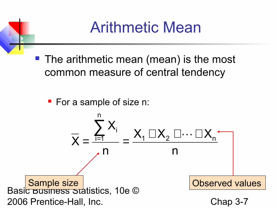
Arithmetic Mean

The arithmetic mean (mean) is the most common measure of central tendency

For a sample of size n:

Sample size

n

XXX

n

XX n21

n

1ii +++==

∑=

Observed values


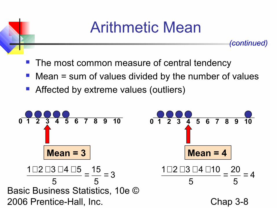
Arithmetic Mean

The most common measure of central tendency Mean = sum of values divided by the number of values Affected by extreme values (outliers)

(continued)

0 1 2 3 4 5 6 7 8 9 10

Mean = 3

0 1 2 3 4 5 6 7 8 9 10

Mean = 4

35

15

5

54321 ==++++4

5

20

5

104321 ==++++


Median

In an ordered array, the median is the “middle” number (50% above, 50% below)

Not affected by extreme values

0 1 2 3 4 5 6 7 8 9 10

Median = 3

0 1 2 3 4 5 6 7 8 9 10

Median = 3


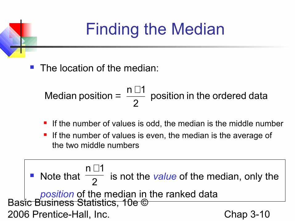
Finding the Median

The location of the median:

If the number of values is odd, the median is the middle number If the number of values is even, the median is the average of

the two middle numbers

Note that is not the value of the median, only the

position of the median in the ranked data

dataorderedtheinposition2

1npositionMedian

+=

2

1n +


Mode

A measure of central tendency Value that occurs most often Not affected by extreme values Used for either numerical or categorical

(nominal) data There may may be no mode There may be several modes

0 1 2 3 4 5 6 7 8 9 10 11 12 13 14

Mode = 9

0 1 2 3 4 5 6

No Mode


Five houses on a hill by the beach

Review Example

$2,000 K

$500 K

$300 K

$100 K

$100 K

House Prices:

$2,000,000 500,000 300,000 100,000 100,000


Review Example:Summary Statistics

Mean: ($3,000,000/5)

= $600,000

Median: middle value of ranked data

= $300,000

Mode: most frequent value = $100,000

House Prices:

$2,000,000 500,000 300,000 100,000 100,000

Sum $3,000,000


Mean is generally used, unless extreme values (outliers) exist

Then median is often used, since the median is not sensitive to extreme values. Example: Median home prices may be

reported for a region – less sensitive to outliers

Which measure of location is the “best”?


Quartiles

Quartiles split the ranked data into 4 segments with an equal number of values per segment

25% 25% 25% 25%

The first quartile, Q1, is the value for which 25% of the observations are smaller and 75% are larger

Q2 is the same as the median (50% are smaller, 50% are larger)

Only 25% of the observations are greater than the third quartile

Q1 Q2 Q3


Quartile Formulas

Find a quartile by determining the value in the appropriate position in the ranked data, where

First quartile position: Q1 = (n+1)/4

Second quartile position: Q2 = (n+1)/2 (the median position)

Third quartile position: Q3 = 3(n+1)/4

where n is the number of observed values


(n = 9)

Q1 is in the (9+1)/4 = 2.5 position of the ranked data

so use the value half way between the 2nd and 3rd values,

so Q1 = 12.5

Quartiles

Sample Data in Ordered Array: 11 12 13 16 16 17 18 21 22

Example: Find the first quartile

Q1 and Q3 are measures of noncentral location Q2 = median, a measure of central tendency


(n = 9)

Q1 is in the (9+1)/4 = 2.5 position of the ranked data,

so Q1 = 12.5

Q2 is in the (9+1)/2 = 5th position of the ranked data,

so Q2 = median = 16

Q3 is in the 3(9+1)/4 = 7.5 position of the ranked data,

so Q3 = 19.5

Quartiles

Sample Data in Ordered Array: 11 12 13 16 16 17 18 21 22

Example:(continued)


Geometric Mean

Geometric mean Used to measure the rate of change of a variable

over time

Geometric mean rate of return Measures the status of an investment over time

Where Ri is the rate of return in time period i

n/1n21G )XXX(X ×××=

1)]R1()R1()R1[(R n/1n21G −+××+×+=


Example

An investment of $100,000 declined to $50,000 at the end of year one and rebounded to $100,000 at end of year two:

000,100$X000,50$X000,100$X 321 ===

50% decrease 100% increase

The overall two-year return is zero, since it started and ended at the same level.


Example

Use the 1-year returns to compute the arithmetic mean and the geometric mean:

%0111)]2()50[(.

1%))]100(1(%))50(1[(

1)]R1()R1()R1[(R

2/12/1

2/1

n/1n21G

=−=−×=

−+×−+=

−+××+×+=

%252

%)100(%)50(X =+−=

Arithmetic mean rate of return:

Geometric mean rate of return:

Misleading result

More accurate result

(continued)


Same center, different variation

Measures of Variation

Variation

Variance Standard Deviation


Range Interquartile Range

Measures of variation give information on the spread or variability of the data values.


Range

Simplest measure of variation Difference between the largest and the smallest

values in a set of data:

Range = Xlargest – Xsmallest

0 1 2 3 4 5 6 7 8 9 10 11 12 13 14

Range = 14 - 1 = 13

Example:


Ignores the way in which data are distributed

Sensitive to outliers

7 8 9 10 11 12

Range = 12 - 7 = 5

7 8 9 10 11 12

Range = 12 - 7 = 5

Disadvantages of the Range

1,1,1,1,1,1,1,1,1,1,1,2,2,2,2,2,2,2,2,3,3,3,3,4,5

1,1,1,1,1,1,1,1,1,1,1,2,2,2,2,2,2,2,2,3,3,3,3,4,120

Range = 5 - 1 = 4

Range = 120 - 1 = 119


Interquartile Range

Can eliminate some outlier problems by using the interquartile range

Eliminate some high- and low-valued observations and calculate the range from the remaining values

Interquartile range = 3rd quartile – 1st quartile = Q3 – Q1


Interquartile Range

Median(Q2)

XmaximumX

minimum Q1 Q3

Example:

25% 25% 25% 25%

12 30 45 57 70

Interquartile range = 57 – 30 = 27


Average (approximately) of squared deviations of values from the mean

Sample variance:

Variance

1-n

)X(XS

n

1i

2i

2∑

=

−=

Where = mean

n = sample size

Xi = ith value of the variable X

X


Standard Deviation

Most commonly used measure of variation Shows variation about the mean Is the square root of the variance Has the same units as the original data

Sample standard deviation:

1-n

)X(XS

n

1i

2i∑

=

−=


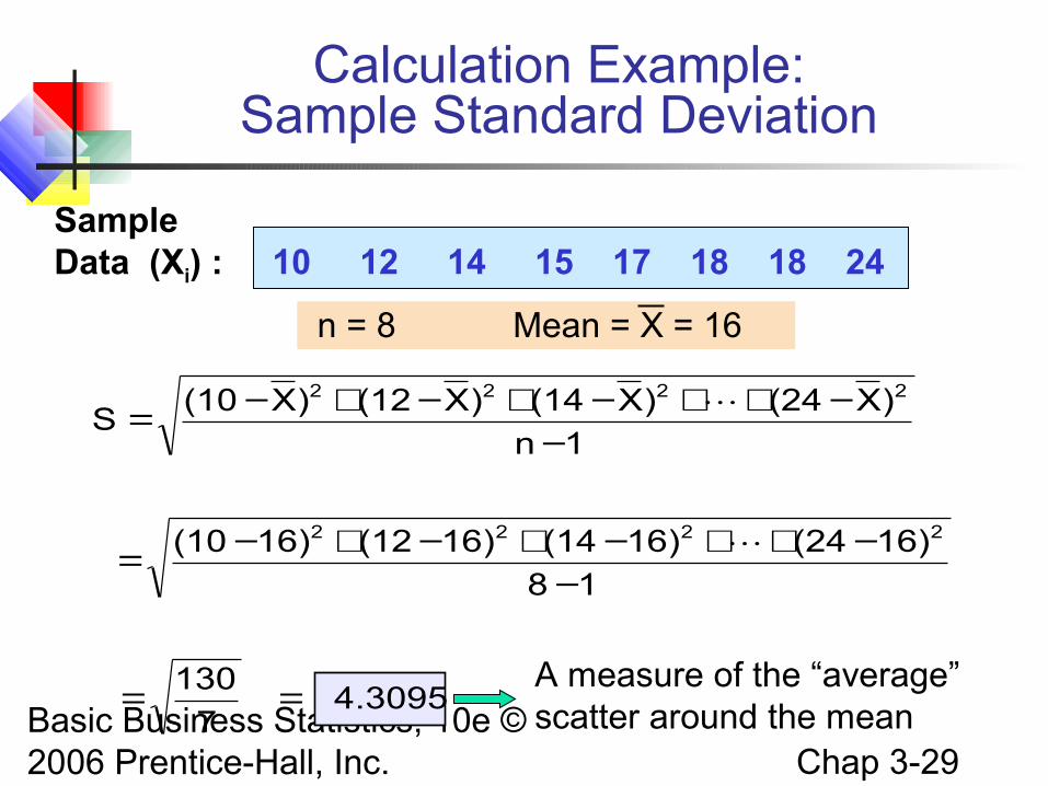
Calculation Example:Sample Standard Deviation

Sample Data (Xi) : 10 12 14 15 17 18 18 24

n = 8 Mean = X = 16

4.30957

130

18

16)(2416)(1416)(1216)(10

1n

)X(24)X(14)X(12)X(10S

2222

2222

==

−−++−+−+−=

−−++−+−+−=

A measure of the “average” scatter around the mean


Measuring variation

Small standard deviation

Large standard deviation


Comparing Standard Deviations

Mean = 15.5 S = 3.338 11 12 13 14 15 16 17 18 19 20 21

11 12 13 14 15 16 17 18 19 20 21

Data B

Data A

Mean = 15.5 S = 0.926

11 12 13 14 15 16 17 18 19 20 21

Mean = 15.5 S = 4.567

Data C


Advantages of Variance and Standard Deviation

Each value in the data set is used in the calculation

Values far from the mean are given extra weight (because deviations from the mean are squared)



Measures relative variation Always in percentage (%) Shows variation relative to mean Can be used to compare two or more sets of

data measured in different units

100%X

SCV ⋅

=


Comparing Coefficient of Variation

Stock A: Average price last year = $50 Standard deviation = $5

Stock B: Average price last year = $100 Standard deviation = $5

Both stocks have the same standard deviation, but stock B is less variable relative to its price

10%100%$50

$5100%

X

SCVA =⋅=⋅

=

5%100%$100

$5100%

X

SCVB =⋅=⋅

=


Z Scores

A measure of distance from the mean (for example, a Z-score of 2.0 means that a value is 2.0 standard deviations from the mean)

The difference between a value and the mean, divided by the standard deviation

A Z score above 3.0 or below -3.0 is considered an outlier

S

XXZ

−=


Z Scores

Example: If the mean is 14.0 and the standard deviation is 3.0,

what is the Z score for the value 18.5?

The value 18.5 is 1.5 standard deviations above the mean

(A negative Z-score would mean that a value is less than the mean)

1.53.0

14.018.5

S

XXZ =−=−=

(continued)


Shape of a Distribution

Describes how data are distributed Measures of shape

Symmetric or skewed

Mean = Median Mean < Median Median < Mean

Right-SkewedLeft-Skewed Symmetric


Using Microsoft Excel

Descriptive Statistics can be obtained from Microsoft® Excel

Use menu choice:

tools / data analysis / descriptive statistics

Enter details in dialog box


Using Excel

Use menu choice:

tools / data analysis /

descriptive statistics


Enter dialog box details

Check box for summary statistics

Click OK

Using Excel(continued)


Excel output

Microsoft Excel

descriptive statistics output,

using the house price data:

House Prices:

$2,000,000 500,000 300,000 100,000 100,000


Numerical Measures for a Population

Population summary measures are called parameters

The population mean is the sum of the values in the

population divided by the population size, N

N

XXX

N

XN21

N

1ii +++==µ

∑=

μ = population mean

N = population size


Where


Average of squared deviations of values from the mean

Population variance:

Population Variance

N

μ)(Xσ

N

1i

2i

2∑

=

−=

Where μ = population mean

N = population size



Population Standard Deviation

Most commonly used measure of variation Shows variation about the mean Is the square root of the population variance Has the same units as the original data

Population standard deviation:

N

μ)(Xσ

N

1i

2i∑

=

−=


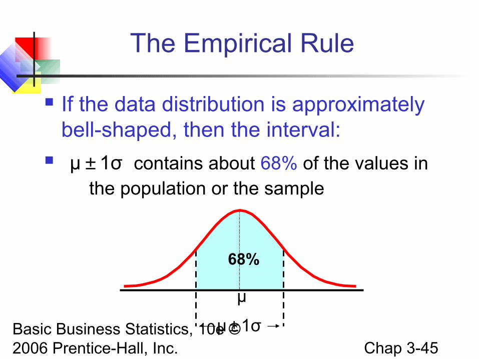
If the data distribution is approximately bell-shaped, then the interval:

contains about 68% of the values in the population or the sample

The Empirical Rule

1σμ ±

μ

68%

1σμ ±


contains about 95% of the values in the population or the sample

contains about 99.7% of the values in the population or the sample

The Empirical Rule

2σμ ±

3σμ ±

3σμ ±

99.7%95%

2σμ ±


Regardless of how the data are distributed, at least (1 - 1/k2) x 100% of the values will fall within k standard deviations of the mean (for k > 1)

Examples:

(1 - 1/12) x 100% = 0% ……..... k=1 (μ ± 1σ)

(1 - 1/22) x 100% = 75% …........ k=2 (μ ± 2σ)

(1 - 1/32) x 100% = 89% ………. k=3 (μ ± 3σ)

Chebyshev Rule

withinAt least


Approximating the Mean from a Frequency Distribution

Sometimes only a frequency distribution is available, not the raw data

Use the midpoint of a class interval to approximate the values in that class

Where n = number of values or sample size c = number of classes in the frequency distribution

mj = midpoint of the jth class

fj = number of values in the jth class

n

fm

X

c

1jjj∑

==


Approximating the Standard Deviation from a Frequency Distribution

Assume that all values within each class interval are located at the midpoint of the class

Approximation for the standard deviation from a frequency distribution:

1-n

f )X(m

S

c

1jj

2j∑

=

−=


Exploratory Data Analysis

Box-and-Whisker Plot: A Graphical display of data using 5-number summary:

Minimum -- Q1 -- Median -- Q3 -- Maximum

Example:

Minimum 1st Median 3rd Maximum Quartile Quartile

Minimum 1st Median 3rd Maximum Quartile Quartile

25% 25% 25% 25%


Shape of Box-and-Whisker Plots

The Box and central line are centered between the endpoints if data are symmetric around the median

A Box-and-Whisker plot can be shown in either vertical or horizontal format

Min Q1 Median Q3 Max


Distribution Shape and Box-and-Whisker Plot

Right-SkewedLeft-Skewed Symmetric

Q1 Q2 Q3 Q1 Q2 Q3 Q1 Q2 Q3


Box-and-Whisker Plot Example

Below is a Box-and-Whisker plot for the following data:

0 2 2 2 3 3 4 5 5 10 27

The data are right skewed, as the plot depicts

0 2 3 5 270 2 3 5 27

Min Q1 Q2 Q3 Max


The Sample Covariance

The sample covariance measures the strength of the linear relationship between two variables (called bivariate data)

The sample covariance:

Only concerned with the strength of the relationship

No causal effect is implied

1n

)YY)(XX()Y,X(cov

n

1iii

−

−−=

∑=


Covariance between two random variables:

cov(X,Y) > 0 X and Y tend to move in the same direction

cov(X,Y) < 0 X and Y tend to move in opposite directions

cov(X,Y) = 0 X and Y are independent

Interpreting Covariance


Coefficient of Correlation

Measures the relative strength of the linear relationship between two variables

Sample coefficient of correlation:

where

YXSS

Y),(Xcovr =

1n

)X(XS

n

1i

2i

X −

−=

∑=

1n

)Y)(YX(XY),(Xcov

n

1iii

−

−−=

∑=

1n

)Y(YS

n

1i

2i

Y −

−=

∑=


Features of Correlation Coefficient, r

Unit free

Ranges between –1 and 1

The closer to –1, the stronger the negative linear

relationship

The closer to 1, the stronger the positive linear

relationship

The closer to 0, the weaker the linear relationship


Scatter Plots of Data with Various Correlation Coefficients

Y

X

Y

X

Y

X

Y

X

Y

X

r = -1 r = -.6 r = 0

r = +.3r = +1

Y

Xr = 0


Using Excel to Find the Correlation Coefficient

Select Tools/Data Analysis

Choose Correlation from the selection menu

Click OK . . .


Using Excel to Find the Correlation Coefficient

Input data range and select appropriate options

Click OK to get output

(continued)


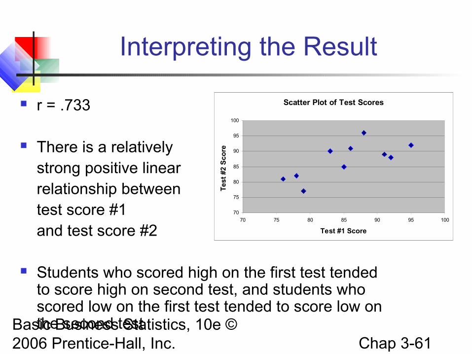
Interpreting the Result

r = .733

There is a relatively strong positive linear relationship between test score #1 and test score #2

Students who scored high on the first test tended to score high on second test, and students who scored low on the first test tended to score low on the second test

Scatter Plot of Test Scores

70

75

80

85

90

95

100

70 75 80 85 90 95 100

Test #1 ScoreT

est

#2 S

core


Pitfalls in Numerical Descriptive Measures

Data analysis is objective Should report the summary measures that best meet

the assumptions about the data set

Data interpretation is subjective Should be done in fair, neutral and clear manner


Ethical Considerations

Numerical descriptive measures:

Should document both good and bad results Should be presented in a fair, objective and

neutral manner Should not use inappropriate summary

measures to distort facts


Chapter Summary

Described measures of central tendency Mean, median, mode, geometric mean

Discussed quartiles Described measures of variation

Range, interquartile range, variance and standard deviation, coefficient of variation, Z-scores

Illustrated shape of distribution Symmetric, skewed, box-and-whisker plots


Chapter Summary

Discussed covariance and correlation

coefficient

Addressed pitfalls in numerical descriptive

measures and ethical considerations

(continued)

Bbs10 ppt ch03

Education

Transcript of Bbs10 ppt ch03