Bayesianmethodsforrecoveryanduncertaintyquantification...
48
Bayesian methods for recovery and uncertainty quantification Lecture 1: Recovery Botond Szabó Leiden University Sydney, 23. 04. 2017.
-
Upload
truongdung -
Category
Documents
-
view
216 -
download
0
Transcript of Bayesianmethodsforrecoveryanduncertaintyquantification...

Bayesian methods for recovery and uncertainty quantification
Lecture 1: Recovery
Botond Szabó
Leiden University
Sydney, 23. 04. 2017.

Outline of the tutorial
• Lecture 1: Introduction to Bayesian methods, recovery.
• Lecture 2: Uncertainty quantification in nonparametric Bayes (curve estimation).
• Lecture 3: Uncertainty quantification in high-dimensional Bayesian models(sparsity)
• Seminar talk: Distributed computation: both Bayesian and frequentist aspects.

Outline of Lecture 1
• Motivation
• Frequentist vs. Bayes
• Bayesian methods for recovery• Consistency• Contraction rate
• Examples• Dirichlet process and DP mixtures• Gaussian process priors
• Summary

Motivating Example I
Air France Flight 447 Malaysian Airlines Flight 370

Motivating Example II
Clements et al. (2009)

Motivating Example II
Clements et al. (2009)

Motivating Example II
Clements et al. (2009)
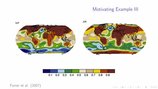
Motivating Example III
Furrer et al. (2007)

Classical statistics
Understanding (certain part of) the world → Model.Use randomness in modeling: {Pθ : θ ∈ Θ}.
Classical (frequentist) statistical model:
X ∼ Pθ0 , θ0 ∈ Θ.
Goal: Recover θ0 from the data.
Inference:• Point estimators (ML estimator, MM, M- and Z-estimators,...).• Confidence sets (uncertainty quantification).• Hypothesis testing (Testing theories about the truth).

Bayesian statistics - history
Thomas Bayes (1702-1761) : Presbyterian minister, formulated a specific case ofBayes theorem. Published post mortem in 1763 by Thomas Price.
Pierre-Simon Laplace (1749-1827) rediscovered Bayes’ argument and applied it togeneral parametric models.
Computational problems in practice. After the development of MCMC methods in the1980/90s, the Bayesian approach became popular again (even in nonparametricproblems).

Bayesian statisticsIncorporate expert knowledge, experience into the statistical model.
Bayesian model:
θ ∼ Π (prior), X |θ ∼ Pθ
(The prior knowledge is expressed through the prior distribution Π.)
Goal: Update our belief about θ from the data.
Inference:
• Compute the posterior distribution Π(·|X )
• Use Bayes theorem:
Π(B|X ) =
∫B pθ(X )dΠ(θ)∫Θ pθ(X )dΠ(θ)
, B ⊂ Θ.

Bayes: pros and cons
Advantages Disadvantages
Conceptual simplicity. Subjective (choice of the prior).
Natural way to express expert knowledge. Difficult to come up with “honest” prior.
Combining and including all information(data) about the problem.
Posterior might heavily depend on the prior.
Update your body of knowledge at any time. Gives room to misinterpretation.
Can be applied even with small amount ofdata.
Computationally intense.
Heavy computational machinery (MCMC,ABC,..).
Simulation based techniques provide only ap-proximations and can be slow.

Bayes vs. Frequentist
Schools: Frequentist Bayes
Model: X ∼ Pθ0 , θ0 ∈ Θ θ ∼ Π (prior), X |θ ∼ Pθ
Goal: Recover θ0: Update our belief about θ:Estimator θ(X ) Posterior: θ|X
Frequentist Bayes
Investigate Bayesian techniques from frequentist perspective, i.e. assume that thereexists a true θ0 and investigate the behaviour of the posterior Π(·|X ).

Toy example: Bayes vs. FrequentistExample: We have a coin, with probability θ to turn up heads, and we flip it 100times. Suppose that we get head 22 times. What can we say about θ?
Frequentist approach: The number of heads has a binomial distribution, withparameters n = 100 and θ. We can estimate θ by θ = 22/100.
Bayesian approach: Endow θ with uniform prior on [0, 1]. Then the posteriordistribution is Beta(23,79). (The posterior mean is 23/102.)

Frequentist Bayes I
Posterior consistency: for all ε > 0
Π(θ : dn(θ, θ0) ≤ ε |X (n))Pθ0→ 1.
Posterior contraction rate: The fastest εn > 0:
Π(θ : dn(θ, θ0) ≤ εn |X (n))Pθ0→ 1
Remark: There exists estimator θn with risk εn:
Take the center of a (nearly) smallest ball that contains posterior mass at least 1/2satisfies d(θn, θ0) = OPn
θ0(εn).

Frequentist Bayes II
Credible set: a set Cn satisfying
Π(θ ∈ Cn |X (n)) = 0.95.
Typically take balls centered around the posterior mean
Cn = {θ : dn(θ, θn) ≤ ρn}, for appropriate radius ρn
Is it a confidence set, i.e. do we have frequentist coverage
Pθ(θ0 ∈ Cn) ≥ 0.95?

Frequentist Bayes II
Credible set: a set Cn satisfying
Π(θ ∈ Cn |X (n)) = 0.95.
Typically take balls centered around the posterior mean
Cn = {θ : dn(θ, θn) ≤ ρn}, for appropriate radius ρn
Is it a confidence set, i.e. do we have frequentist coverage
Pθ(θ0 ∈ Cn) ≥ 0.95?

Parametric Bayes - Bernstein-von Mises
Assume that we observe iid sample X (n) = {X1, ..,Xn} from density pθ0 for someθ0 ∈ Rd , d > 0 fixed.
Theorem: [Bernstein-von Mises] For any prior which has positive mass around θ0 wehave ∥∥Π( · |X (n))− N( · , θn, I−1
θ0/n)∥∥TV
Pθ0→ 0,
where θn is an estiamtor satisfying√n(θn − θ0)→ N(0, I−1
θ0).
Consequence: Optimal, parametric contraction rate 1/√n and credible sets are
asymptotically confidence sets.

Nonparametric Bayes - Consistency IBayesian model:
X (n) = {X1, ...,Xn}|θ ∼ Pθ, θ ∼ Π(·).
Does
Π(θ : dn(θ, θ0) ≤ ε |X (n))Pθ0→ 1
hold for all ε > 0? (a.s. convergence: strong consistency)
• Prior a.s. the posterior is consistent; Doob (1949).
• BUT prior zero set can be arbitrarily large from topological point of view.
• Goal: Consistency for every parameter θ.
• Doesn’t necessarily hold (various natural examples), Diaconis and Freedman(1963,1965).

Nonparametric Bayes - Consistency II
Definition: [KL-property] θ0 is said to possess the Kullback-Leibler property relative toΠ(·) if for every ε > 0
Π(θ : KL(θ0, θ) ≤ ε) > 0, where KL(θ0, θ) =
∫pθ0 log
pθ0pθ.
Theorem [Schwartz (1965)]: If θ0 has KL-property and for every neighbourhood U of
θ0 there exist tests ϕn such that
P(n)θ0ϕn → 0 and sup
θ∈UcP
(n)θ (1− ϕn)→ 0,
then Π(· |X (n)) is strongly consistent.
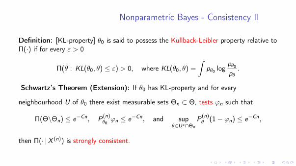
Nonparametric Bayes - Consistency II
Definition: [KL-property] θ0 is said to possess the Kullback-Leibler property relative toΠ(·) if for every ε > 0
Π(θ : KL(θ0, θ) ≤ ε) > 0, where KL(θ0, θ) =
∫pθ0 log
pθ0pθ.
Schwartz’s Theorem (Extension): If θ0 has KL-property and for every
neighbourhood U of θ0 there exist measurable sets Θn ⊂ Θ, tests ϕn such that
Π(Θ\Θn) ≤ e−Cn, P(n)θ0ϕn ≤ e−Cn, and sup
θ∈Uc∩Θn
P(n)θ (1− ϕn) ≤ e−Cn,
then Π(· |X (n)) is strongly consistent.

Nonparametric Bayes - Contraction rates I
Notations:• Entropy (model complexity): N(ε,Θ, ‖ · ‖) denotes the number of ε-balls neededto cover Θ
• Second moment of log-likelihood ratio: V (θ0, θ) =∫pθ0 log
2 pθ0pθ
.

Nonparametric Bayes - Contraction rates II
Theorem [Ghoshal, Ghosh, van der Vaart (2000)]: Assume that X (n) = {X1, ...,Xn} isiid data from Pθ0 and that there exists Θn ⊂ Θ such that
logN(εn,Θn, h)≤nε2nΠ(Θ\Θn)≤ exp(−(C + 4)nε2n)
Π(θ : −KL(θ0, θ)≤ ε2n,V (θ0, θ) ≤ ε2n)≥ exp(−Cnε2n).
Then for sufficiently large M, we have that
Π(θ : h(Pθ,Pθ0)≤ Mεn|X (n))Pθ0→ 1.

Dirichlet processDefinition [Dirichlet distribution]: (θ1, ..., θk) possesses a Dirichlet distributionDir(k , α1, ...., αk), if it has density on the k dimensional simplex (wrt the Lebesguemeasure):
p(θ1, ..., θk) ∝ θα1−11 × ...× θαk−1
k .
Definition [Dirichlet process]: A random measure P on a measurable space (X ,X ) is
a Dirichlet process with base measure α, if for every finite partition A1, ...,Ak of X wehave that (
P(A1),P(A2), ...,P(Ak))∼ Dir
(k, α(A1), α(A2), ..., α(Ak)
).
Theorem [Sethuraman (1994)]: If θ1, θ2...iid∼ α, Y1,Y2, ...
iid∼ Be(1,M) and
Vj = Yj∏j−1
i=1(1− Yi ) then
P =∞∑j=1
Vjδθj ∼ DP(Mα).

Dirichlet process: example
α = N(0, 2) α = 10N(0.2)
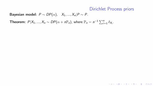
Dirichlet Process priorsBayesian model: P ∼ DP(α), X1, ...,Xn|P ∼ P .
Theorem: P|X1, ...,Xn ∼ DP(α + nPn), where Pn = n−1∑ni=1 δXi
.
Theorem: The posterior distribution of P(A) satisfies the Bernstein-von Misestheorem: ∥∥∥Π
(P(A) |X1, ...,Xn
)− N
(Pn(A),
P0(A)(1− P0(A))
n
)∥∥∥TV
P0→ 0

Dirichlet Process priorsBayesian model: P ∼ DP(α), X1, ...,Xn|P ∼ P .
Theorem: P|X1, ...,Xn ∼ DP(α + nPn), where Pn = n−1∑ni=1 δXi
.
Theorem: The posterior distribution of P(A) satisfies the Bernstein-von Misestheorem: ∥∥∥Π
(P(A) |X1, ...,Xn
)− N
(Pn(A),
P0(A)(1− P0(A))
n
)∥∥∥TV
P0→ 0

Dirichlet Process mixturesThe Dirichlet process is discrete a.s. ⇒ Not suitable for density estimation.
Dirichlet process mixture of normals:
X1, ...,Xniid∼ pF ,σ(·) =
∫R
1σϕ( · − z
σ
)dF (z), F ∼ DP(α), σ ∼ π.

Dirichlet Process mixtures II
Definition [Holder smoothness]: f0 is β-Holder smooth if f0 is bβc times continuouslydifferentiable and the bβcth derivative satisfies
|f bβc0 (x)− fbβc0 (y)| ≤ c |x − y |β−bβc, for every x , y .
Theorem: Suppose that p0 is β-Holder smooth satisfying p0(x) ≤ c1e−c2xc3 , then the
posterior distribution resulting from the DP mixture of normals priors pF ,σ(·) withσ ∼ IΓ(c4, c5) (and base measure α(|z | > M) ≤ c6e
−c7Mc8 with ci > 0, ∀i)
Π(p : ‖p − p0‖1 ≤ Mn−2β
1+2β (log n)δ|X1, ...,Xn)Pθ0→ 1,
for some M, δ > 0

Gaussian processDefinition [Gaussian process]: Wt , t ∈ T is a Gaussian process if for every finite sett1, ..., tk the random vector (Wt1 , ...,Wtk ) is multivariate Gaussian distributed.
The Gaussian process is determined by the mean and covariance functions"
t 7→ EWt and (t, s) 7→ cov(Wt ,Ws).

Applying GP priors
• Nonparametric (fixed design) regression:
Yi |f , xiind∼ N(f (xi ), 1), i = 1, ..., n, f ∼W .
• Density estimation:
Yi |fiid∼ f , f ∼ eW∫
eWtdt.
• Nonparametric classification:
Yi |p, xiind∼ Bernoulli
(q(xi )
), i = 1, ..., n, q ∼ eW
1 + eW.

Contraction rates for GP priors
View the GP W as measurable map into a Banach space (B, ‖ · ‖).
Theorem [vd Vaart and v Zanten (2008)] Assume that εn > 0 satisfies
Π(‖W − w0‖≤εn)≥e−nε2n .
Then if statistical distances on the model combines appropriately with the norm ‖ · ‖ ofB, then
Π(‖W − w0‖ ≤ Mnεn|Y1, ...,Yn)Pnw0→ 1,
for any Mn tending to infinity.
Examples: regression (empirical norm vs. L2-norm), density (hellinger vs L∞),classification (empirical hellinger vs. L2).

GP small ball probability I
Alternative formulation of the prior small ball condition:
− logΠ(‖W ‖ ≤ εn) ≤ nε2n and infh∈H: ‖h−w0‖≤εn
‖h‖2H ≤ nε2n,
where H is the RKHS of W .
Example 1: Let w0 ∈ Hβ(M) and W the α− 1/2 integrated Brownian motion
− logΠ(‖W ‖∞ ≤ ε) ∼ ε−1/α ⇒ εn & n−α
1+2α ,
infh∈H: ‖h−w0‖∞≤εn
‖h‖2H . n1+2(α−β)
1+2α ⇒ εn & n−β
1+2α
To achieve the rate n−β/(1+2β) one has to choose α = β.

GP small ball probability II
Example 2: Centered GP with square exponential covariance kernel:
cov(Gt ,Gs) = e−‖s−t‖2, s, t ∈ R.

GP small ball probability IIRescaled square exponential GP: W τ
t = Gt/τ .
Let w0 ∈ Hβ(M) then
− logΠ(‖W τ‖∞ ≤ ε) . τ−1 log2(1
τ2ε2),
supw0∈Hβ(M)
infh∈H: ‖h−w0‖∞≤εn
‖h‖2Hτ . τ−1
hence taking τ = n1/(1+2β) results εn . n−β/(1+2β)(log n)δ.