arX

iv:1

210.

0333

v2 [

stat

.CO

] 2

0 Fe

b 20

13

Bayesian computing with INLA: new features

Thiago G. Martins∗, Daniel Simpson, Finn Lindgren & Havard Rue

Department of Mathematical Sciences

Norwegian University of Science and Technology

N-7491 Trondheim, Norway

February 21, 2013

Abstract

The INLA approach for approximate Bayesian inference for latent Gaussian models has

been shown to give fast and accurate estimates of posterior marginals and also to be a valuable

tool in practice via the R-package R-INLA. In this paper we formalize new developments in

the R-INLA package and show how these features greatly extend the scope of models that

can be analyzed by this interface. We also discuss the current default method in R-INLA

to approximate posterior marginals of the hyperparameters using only a modest number of

evaluations of the joint posterior distribution of the hyperparameters, without any need for

numerical integration.

Keywords: Approximate Bayesian inference, INLA, Latent Gaussian models

1 Introduction

The Integrated Nested Laplace Approximation (INLA) is an approach proposed by Rue et al.

(2009) to perform approximate fully Bayesian inference on the class of latent Gaussian models

(LGMs). INLA makes use of deterministic nested Laplace approximations and, as an algorithm

tailored to the class of LGMs, it provides a faster and more accurate alternative to simulation-

based MCMC schemes. This is demonstrated in a series of examples ranging from simple to

complex models in Rue et al. (2009). Although the theory behind INLA has been well established

in Rue et al. (2009), the INLA method continues to be a research area in active development.

Designing a tool that allows the user the flexibility to define their own model with a relatively

∗Corresponding author.

1

easy to use interface is an important factor for the success of any approximate inference method.

The R package INLA, hereafter refereed as R-INLA, provides this interface and allow users to

specify and perform inference on complex LGMs.

The breadth of classical Bayesian problems covered under the LGM framework, and therefore

handled by INLA, is — when coupled with the user-friendly R-INLA interface — a key element in

the success of the INLA methodology. For example, INLA has been shown to work well with gen-

eralized linear mixed models (GLMM) (Fong et al., 2010), spatial GLMM (Eidsvik et al., 2009),

Bayesian quantile additive mixed models (Yue and Rue, 2011), survival analysis (Martino et al.,

2011b), stochastic volatility models (Martino et al., 2011a), generalized dynamic linear models

(Ruiz-Cardenas et al., 2011), change point models where data dependency is allowed within seg-

ments (Wyse et al., 2011), spatio-temporal disease mapping models (Schrodle and Held, 2011),

models to complex spatial point pattern data that account for both local and global spatial

behavior (Illian et al., 2011), and so on.

There has also been a considerable increase in the number of users that have found in

INLA the possibility to fit models that they were otherwise unable to fit. More interestingly,

those users come from areas that are sometimes completely unrelated to each other, such as

econometrics, ecology, climate research, etc. Some examples are bi-variate meta-analysis of

diagnostic studies (Paul et al., 2010), detection of under-reporting of cases in an evaluation

of veterinary surveillance data (Schrodle et al., 2011), investigation of geographic determinants

of reported human Campylobacter infections in Scotland (Bessell et al., 2010), the analysis of

the impact of different social factors on the risk of acquiring infectious diseases in an urban

setting (Wilking et al., 2012), analysis of animal space use metrics (Johnson et al., 2011), animal

models used in evolutionary biology and animal breeding to identify the genetic part of traits

(Holand et al., 2011), analysis of the relation between biodiversity loss and disease transmission

across a broad, heterogeneous ecoregion (Haas et al., 2011), identification of areas in Toronto

where spatially varying social or environmental factors could be causing higher incidence of lupus

than would be expected given the population (Li et al., 2011), and spatio-temporal modeling of

particulate matter concentration in the North-Italian region Piemonte (Cameletti et al., 2012).

The relative black-box format of INLA allows it to be embedded in external tools for a more

integrated data analysis. For example, Beale et al. (2010) mention that INLA has been used by

tools embedded in a Geographical Information System (GIS) to evaluate the spatial relationships

between health and the environment data. The model selection measures available in INLA are

also something very much appreciated in the applied work mentioned so far. Such quantities

include marginal likelihood, deviance information criterion (DIC) (Spiegelhalter et al., 2002),

2

and other predictive measures.

Some extensions to the work of Rue et al. (2009) have also been presented in the literature;

Hosseini et al. (2011) extends the INLA approach to fit spatial GLMM with skew normal pri-

ors for the latent variables instead of the more standard normal priors, Sørbye and Rue (2010)

extend the use of INLA to joint inference and present an algorithm to derive analytical simulta-

neous credible bands for subsets of the latent field based on approximating the joint distribution

of the subsets by multivariate Gaussian mixtures, Martins and Rue (2012) extend INLA to fit

models where independent components of the latent field can have non-Gaussian distributions,

and Cseke and Heskes (2011) discuss variations of the classic Laplace-approximation idea based

on alternative Gaussian approximations (see also (Rue et al., 2009, pp. 386-7) for a discussion

on this issue).

A lot of advances have been made in the area of spatial and spatial-temporal models,

Eidsvik et al. (2011) address the issue of approximate Bayesian inference for large spatial datasets

by combining the use of prediction process models as a reduced-rank spatial process to diminish

the dimensionality of the model and the use of INLA to fit this reduced-rank models. INLA

blends well with the work of Lindgren et al. (2011) where an explicit link between Gaussian

Fields (GFs) and Gaussian Markov Random Fields (GMRFs) allow the modeling of spatio and

spatio-temporal data to be done with continuously indexed GFs while the computations are

carried out with GMRFs, using INLA as the inferential algorithm.

The INLA methodology requires some expertise in numerical methods and computer pro-

gramming to be implemented, since all procedures required to perform INLA need to be carefully

implemented to achieve a good speed. This can, at first, be considered a disadvantage when

compared with other approximate methods such as (naive) MCMC schemes that are much easier

to implement, at least on a case by case basis. To overcome this, the R-INLA package was devel-

oped to provide an easy to use interface to the stand-alone C coded inla program. 1 To download

the package one only needs one line of R code that can be found on the download section of the

INLA website (http://www.r-inla.org/). In addition, the website contains several worked

out examples, papers and even the complete source code of the project.

In Rue et al. (2009) most of the attention was focused on the computation of the poste-

rior marginal of the elements of the latent field since those are usually the biggest challenge

when dealing with LGMs given the high dimension of the latent field usually found in models

of interest. On the other hand, it was mentioned that the posterior marginal of the unknown

parameters not in the latent field, hereafter refereed as hyperparameters, are obtained via nu-

1The dependency on the stand-alone C program is the reason why R-INLA is not available on CRAN.

3

merical integration of an interpolant constructed from evaluations of the Laplace approximation

of the joint posterior of the hyperparameters already computed in the computation of the poste-

rior marginals of the latent field. However, details of such interpolant were not given. The first

part of this paper will show how to construct this interpolant in a cost-effective way. Besides

that, we will describe the algorithm currently in use in R-INLA package that completely bypass

the need for numerical integration, providing accuracy and scalability.

Unfortunately, when an interface is designed, a compromise must be made between simplicity

and generality, meaning that in order to build a simple to use interface, some models that

could be handled by the INLA method might not be available through that interface, hence not

available to the general user. The second part of this paper will formalize some new developments

already implemented on the R-INLA package and show how these new features greatly extend the

scope of models available through that interface. It is important to keep in mind the difference

between the models that can be analyzed by the INLA method and the models that can be

analyzed through the R-INLA package. The latter is contained within the first, which means

that not every model that can be handled by the INLA method is available through the R-INLA

interface. Therefore, this part of the paper will formalize tools that extend the scope of models

within R-INLA that were already available within the theoretical framework of the INLA method.

Section 2 will present an overview of the latent Gaussian models and of the INLA methodol-

ogy. Section 3 will address the issue of computing the posterior marginal of the hyperparameters

using a novel approach. A number of new features already implemented in the R-INLA package

will be formalized in Section 4 together with examples highlighting their usefulness.

2 Integrated Nested Laplace Approximation

In Section 2.1 we define latent Gaussian models using a hierarchical structure highlighting the

assumptions required to be used within the INLA framework and point out which components

of the model formulation will be made more flexible with the features presented in Section 4.

Section 2.2 gives a brief description of the INLA approach and presents the task of approximating

the posterior marginals of the hyperparameters that will be formalized in Section 3. A basic

description of the R-INLA package is given in Section 2.3 and this is mainly to situate the reader

when going through the extensions in Section 4.

4

2.1 Latent Gaussian models

The INLA framework was designed to deal with latent Gaussian models, where the observation

(or response) variable yi is assumed to belong to a distribution family (not necessarily part of

the exponential family) where some parameter of the family φi is linked to a structured additive

predictor ηi through a link function g(·), so that g(φi) = ηi. The structured additive predictor

ηi accounts for effects of various covariates in an additive way:

ηi = α+

nf∑

j=1

f (j)(uji) +

ηβ∑

k=1

βkzki + ǫi, (1)

where {f (j)(·)}’s are unknown functions of the covariates u, used for example to relax linear

relationship of covariates and to model temporal and/or spatial dependence, the {βk}’s representthe linear effect of covariates z and the {ǫi}’s are unstructured terms. Then a Gaussian prior is

assigned to α, {f (j)(·)}, {βk} and {ǫi}.We can also write the model described above using a hierarchical structure, where the first

stage is formed by the likelihood function with conditional independence properties given the

latent field x = (η, α,f ,β) and possible hyperparameters θ1, where each data point {yi, i =1, ..., nd} is connected to one element in the latent field xi. Assuming that the elements of the

latent field connected to the data points are positioned on the first nd elements of x, we have

Stage 1. y|x,θ1 ∼ π(y|x,θ1) =∏nd

i=1 π(yi|xi,θ1).

Two new features relaxing the assumptions of Stage 1 within the R-INLA package will be

presented in Section 4. Section 4.1 will show how to fit models where different subsets of data

come from different sources (i.e. different likelihoods) and Section 4.4 will show how to relax

the assumption that each observation can only depend on one element of the latent field and

allow it to depend on a linear combination of the elements in the latent field.

The conditional distribution of the latent field x given some possible hyperparameters θ2

forms the second stage of the model and has a joint Gaussian distribution,

Stage 2. x|θ2 ∼ π(x|θ2) = N (x;µ(θ2),Q−1(θ2)),

where N (·;µ,Q−1) denotes a multivariate Gaussian distribution with mean vector µ and a pre-

cision matrix Q. In most applications, the latent Gaussian field have conditional independence

properties, which translates into a sparse precision matrix Q(θ2), which is of extreme impor-

tance for the numerical algorithms that will follow. A multivariate Gaussian distribution with

sparse precision matrix is known as a Gaussian Markov Random Field (GMRF) (Rue and Held,

5

2005). The latent field x may have additional linear constraints of the form Ax = e for an k×nmatrix A of rank k, where k is the number of constraints and n the size of the latent field. Stage

2 is very general and can accommodate an enormous number of latent field structures. Sections

4.2, 4.3 and 4.6 will formalize new features of the R-INLA package that gives the user greater

flexibility to define these latent field structure, i.e. enable them to define complex latent fields

from simpler GMRFs building blocks.

The hierarchical model is then completed with an appropriate prior distribution for the

hyperparameters of the model θ = (θ1,θ2)

Stage 3. θ ∼ π(θ).

2.2 INLA methodology

For the hierarchical model described in Section 2.1, the joint posterior distribution of the un-

knowns then reads

π(x,θ|y) ∝ π(θ)π(x|θ)nd∏

i=1

π(yi|xi,θ)

∝ π(θ)|Q(θ)|n/2 exp[− 1

2xTQ(θ)x+

nd∑

i=1

log{π(yi|xi,θ)}]

and the marginals of interest can be defined as

π(xi|y) =∫π(xi|θ,y)π(θ|y)dθ i = 1, ..., n

π(θj|y) =∫π(θ|y)dθ−j j = 1, ...,m

while the approximated posterior marginals of interest π(xi|y), i = 1, .., n and π(θj |y), j =

1, ...,m returned by INLA has the following form

π(xi|y) =∑

k

π(xi|θ(k),y)π(θ(k)|y) ∆θ(k) (2)

π(θj|y) =∫π(θ|y)dθ−j (3)

where {π(θ(k)|y)} are the density values computed during a grid exploration on π(θ|y).Looking at [(2)-(3)], we can see that the method can be divided into three main tasks, firstly

propose an approximation π(θ|y) to the joint posterior of the hyperparameters π(θ|y), secondlypropose an approximation π(xi|θ,y) to the marginals of the conditional distribution of the latent

field given the data and the hyperparameters π(xi|θ,y) and finally explore π(θ|y) on a grid and

use it to integrate out θ in Eq. (2) and θ−j in Eq. (4).

6

Since we don’t have π(θ|y) evaluated at all points required to compute the integral in Eq. (3)

we construct an interpolation I(θ|y) using the density values {π(θ(k)|y)} computed during the

grid exploration on π(θ|y) and approximate (3) by

π(θj |y) =∫I(θ|y)dθ−j. (4)

Details on how to construct such interpolant were not given in Rue et al. (2009). Besides the

description of the interpolation algorithm used to compute Eq. (4), Section 3 will present a

novel approach to compute π(θj|y) that bypass numerical integration.

The approximation used for the joint posterior of the hyperparameters π(θ|y) is

π(θ|y) ∝ π(x,θ,y)

πG(x|θ,y)

∣∣∣∣x=x∗(θ)

(5)

where πG(x|θ,y) is a Gaussian approximation to the full conditional of x obtained by matching

the modal configuration and the curvature at the mode, and x∗(θ) is the mode of the full

conditional for x, for a given θ. Expression (5) is equivalent to the Laplace approximation of

a marginal posterior distribution (Tierney and Kadane, 1986), and it is exact if π(x|y,θ) is a

Gaussian.

For π(xi|θ,y), three options are available, and they vary in terms of speed and accuracy. The

fastest option, πG(xi|θ,y), is to use the marginals of the Gaussian approximation πG(x|θ,y)already computed when evaluating expression (5). The only extra cost to obtain πG(xi|θ,y) isto compute the marginal variances from the sparse precision matrix of πG(x|θ,y), see Rue et al.

(2009) for details. The Gaussian approximation often gives reasonable results, but there can be

errors in the location and/or errors due to the lack of skewness (Rue and Martino, 2007). The

more accurate approach would be to do again a Laplace approximation, denoted by πLA(xi|θ,y),with a form similar to expression (5)

πLA(xi|θ,y) ∝π(x,θ,y)

πGG(x−i|xi,θ,y)

∣∣∣∣x−i=x∗

−i(xi,θ)

, (6)

where x−i represents the vector x with its i-th element excluded, πGG(x−i|xi,θ,y) is the Gaus-

sian approximation to x−i|xi,θ,y and x∗−i(xi,θ) is the modal configuration. A third option

πSLA(xi|θ,y), called simplified Laplace approximation, is obtained by doing a Taylor expan-

sion on the numerator and denominator of expression (6) up to third order, thus correcting the

Gaussian approximation for location and skewness with a much lower cost when compared to

πLA(xi|θ,y). We refer to Rue et al. (2009) for a detailed description of the Gaussian, Laplace

and simplified Laplace approximations to π(xi|θ,y).

7

2.3 R-INLA interface

In this Section we present the general structure of the R-INLA package since the reader will

benefit from this when reading the extensions proposed in Section 4. The syntax for the R-INLA

package is based on the built-in glm function in R, and a basic call starts with

formula = y ~ a + b + a:b + c*d + f(idx1, model1, ...) + f(idx2, model2, ...)

where formula describe the structured additive linear predictor described in Eq. (1). Here, y

is the response variable, the term a + b + a:b + c*d hold similar meaning as in the built-in

glm function in R and are then responsible for the fixed effects specification. The f() terms

specify the general Gaussian random effects components of the model and represent the smooth

functions {f (j)(·)} in Eq. (1). In this case we say that both idx1 and idx2 are latent building

blocks that are combined together to form a joint latent Gaussian model of interest. Once the

linear predictor is specified, a basic call to fit the model with R-INLA takes the following form:

result = inla(formula, data = data.frame(y, a, b, c, d, idx1, idx2),

family = "gaussian")

After the computations the variable result will hold an S3 object of class "inla", from which

summaries, plots, and posterior marginals can be obtained. We refer to the package website

http://www.r-inla.org for more information about model components available to use inside

the f() functions as well as more advanced arguments to be used within the inla() function.

3 On the posterior marginals for the hyperparameters

This Section starts by describing the grid exploration required to integrate out the uncertainty

with respect to θ when computing the posterior marginals of the latent field. It also presents two

algorithms that can be used to compute the posterior marginals of the hyperparameters with

little additional cost by using the points of the joint density of the hyperparameters already

evaluated during the grid exploration.

3.1 Grid exploration

The main focus in Rue et al. (2009) lies on approximating posterior marginals for the latent field.

In this context, π(θ|y) is used to integrate out uncertainty with respect to θ when approximating

π(xi|y). For this task we do not need a detailed exploration of π(θ|y) as long as we are able

8

to select good evaluation points for the numerical solution of Eq. (2). Rue et al. (2009) propose

two different exploration schemes to perform the integration.

Both schemes require a reparametrization of θ-space in order to make the density more

regular, we denote such parametrization as the z-parametrization throughout the paper. Assume

θ = (θ1, . . . , θm) ∈ Rm, which can always be obtained by ad-hoc transformations of each element

of θ, we proceed as follows:

1. Find the mode θ∗ of π(θ|y) and compute the negative Hessian H at the modal configu-

ration

2. Compute the eigen-decomposition Σ = V Λ1/2V T where Σ = H−1

3. Define a new z-variable such that

θ(z) = θ∗ + V Λ1/2z

The variable z = (z1, . . . , zm) is standardized and its components are mutually orthogonal.

At this point, if the dimension of θ is small, say m ≤ 5, Rue et al. (2009) propose to use the

z-parametrization to build a grid covering the area where the density of π(θ|y) is higher. Suchprocedure has a computational cost which grows exponentially with m. It turns out that, when

the goal is π(xi|y), a rather rough grid is enough to give accurate results.

If the dimension of θ is higher, Rue et al. (2009) propose a different approach, named CCD

integration. Here the integration problem is considered as a design problem and, using the mode

θ∗ and the negative Hessian H as a guide, we locate some “points” in the m-dimensional space

which allows us to approximate the unknown function with a second order surface (see Section

6.5 of Rue et al., 2009). The CCD strategy requires much less computational power compared

to the grid strategy but, when the goal is π(xi|y), it still allows to capture variability in the

hyperparameter space when this is too wide to be explored via the grid strategy.

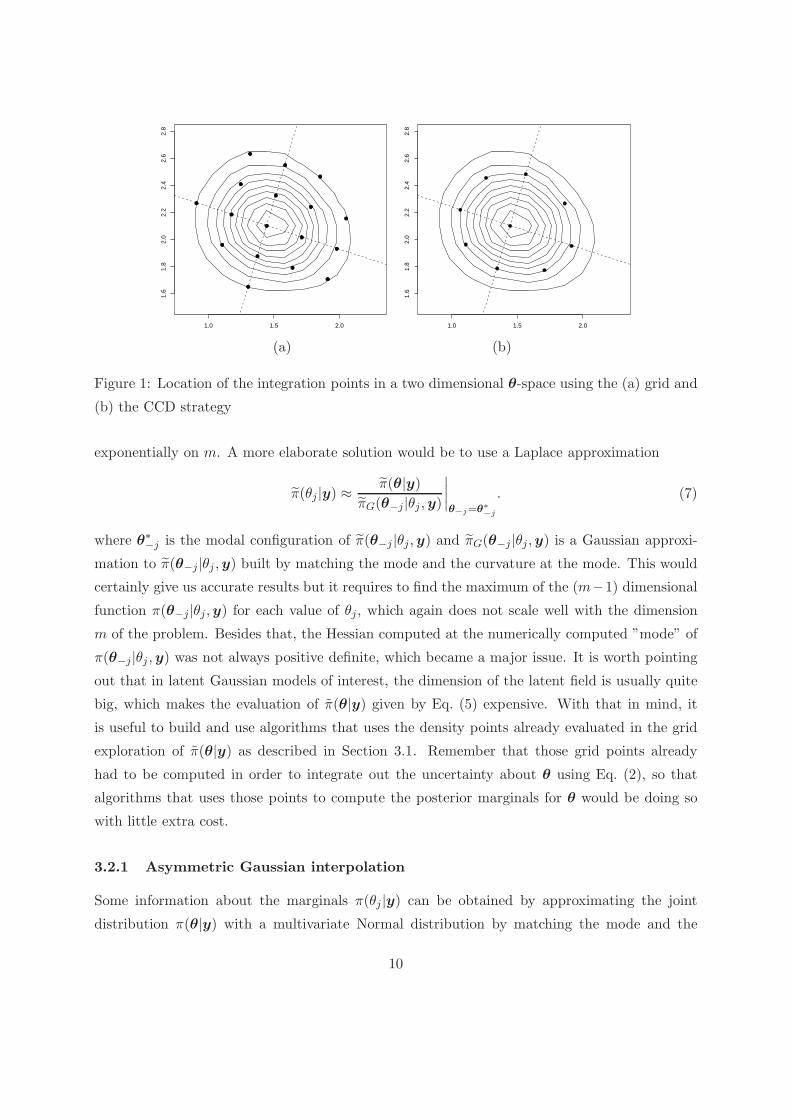
Figure 1 shows the location of the integration points in a two dimensional θ-space using the

grid and the CCD strategy.

3.2 Algorithms for computing π(θj |y)

If the dimension of θ is not too high, it is possible to evaluate π(θ|y) on a regular grid and use the

resulting values to numerical compute the integral in Eq. (3) by summing out the variables θ−j .

Of course this is a naive solution in which the cost to obtain m such marginals would increase

9

1.0 1.5 2.0

1.6

1.8

2.0

2.2

2.4

2.6

2.8

1.0 1.5 2.0

1.6

1.8

2.0

2.2

2.4

2.6

2.8

(a) (b)

Figure 1: Location of the integration points in a two dimensional θ-space using the (a) grid and

(b) the CCD strategy

exponentially on m. A more elaborate solution would be to use a Laplace approximation

π(θj |y) ≈π(θ|y)

πG(θ−j|θj ,y)

∣∣∣∣θ−j=θ∗

−j

. (7)

where θ∗−j is the modal configuration of π(θ−j |θj,y) and πG(θ−j |θj,y) is a Gaussian approxi-

mation to π(θ−j|θj ,y) built by matching the mode and the curvature at the mode. This would

certainly give us accurate results but it requires to find the maximum of the (m−1) dimensional

function π(θ−j|θj,y) for each value of θj, which again does not scale well with the dimension

m of the problem. Besides that, the Hessian computed at the numerically computed ”mode” of

π(θ−j|θj ,y) was not always positive definite, which became a major issue. It is worth pointing

out that in latent Gaussian models of interest, the dimension of the latent field is usually quite

big, which makes the evaluation of π(θ|y) given by Eq. (5) expensive. With that in mind, it

is useful to build and use algorithms that uses the density points already evaluated in the grid

exploration of π(θ|y) as described in Section 3.1. Remember that those grid points already

had to be computed in order to integrate out the uncertainty about θ using Eq. (2), so that

algorithms that uses those points to compute the posterior marginals for θ would be doing so

with little extra cost.

3.2.1 Asymmetric Gaussian interpolation

Some information about the marginals π(θj |y) can be obtained by approximating the joint

distribution π(θ|y) with a multivariate Normal distribution by matching the mode and the

10

curvature at the mode of π(θ|y). Such Gaussian approximation for π(θj |y) comes with no

extra computational effort since the mode θ∗ and the negative Hessian H of π(θ|y) are alreadycomputed in the numerical strategy used to approximate Eq. (2) as described in Section 3.1.

Unfortunately, π(θj|y) can be rather skewed so that a Gaussian approximation is inaccurate.

It is possible to correct the Gaussian approximation for the lack of asymmetry, with minimal

additional costs, as described in the following.

Let z(θ) = (z1(θ), ..., zm(θ)) be the point in the z-parametrization corresponding to θ. We

define the function f(θ) as

f(θ) =m∏

j=1

fj(zj(θ)) (8)

where

fj(z) ∝{

exp(− 1

2(σj+)2z2)

if z ≥ 0

exp(− 1

2(σj−)2z2)

if z < 0.(9)

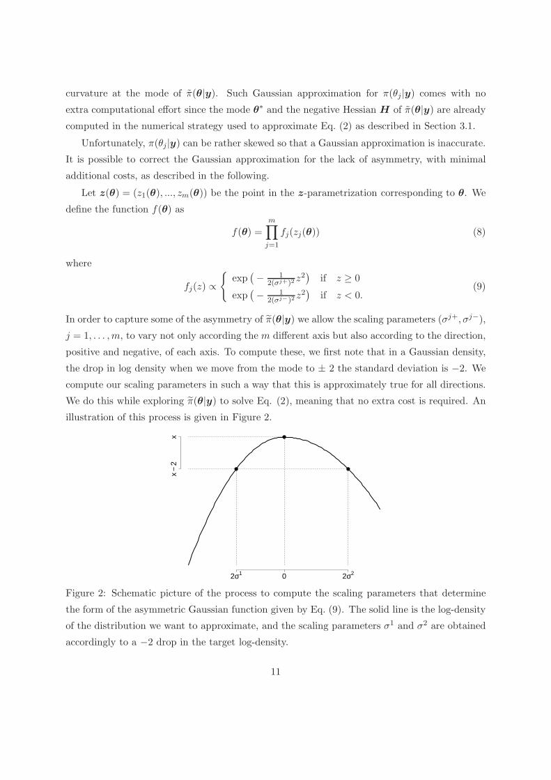
In order to capture some of the asymmetry of π(θ|y) we allow the scaling parameters (σj+, σj−),

j = 1, . . . ,m, to vary not only according the m different axis but also according to the direction,

positive and negative, of each axis. To compute these, we first note that in a Gaussian density,

the drop in log density when we move from the mode to ± 2 the standard deviation is −2. We

compute our scaling parameters in such a way that this is approximately true for all directions.

We do this while exploring π(θ|y) to solve Eq. (2), meaning that no extra cost is required. An

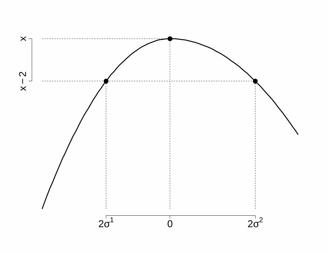
illustration of this process is given in Figure 2.

2σ1 0 2σ2

x−

2x

Figure 2: Schematic picture of the process to compute the scaling parameters that determine

the form of the asymmetric Gaussian function given by Eq. (9). The solid line is the log-density

of the distribution we want to approximate, and the scaling parameters σ1 and σ2 are obtained

accordingly to a −2 drop in the target log-density.

11

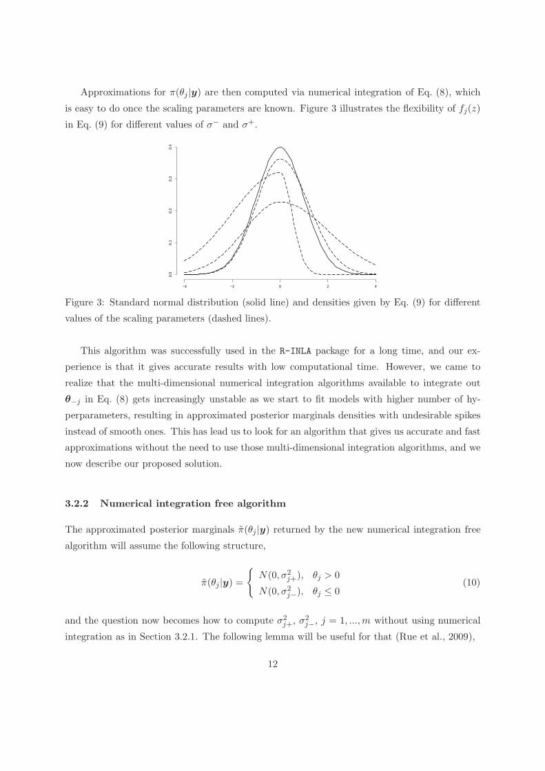
Approximations for π(θj |y) are then computed via numerical integration of Eq. (8), which

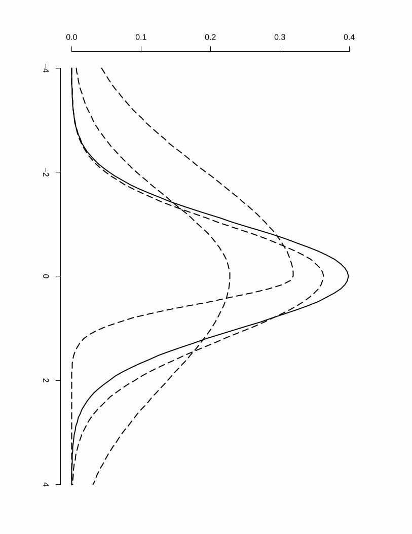
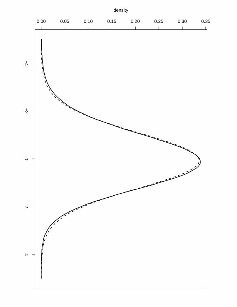
is easy to do once the scaling parameters are known. Figure 3 illustrates the flexibility of fj(z)

in Eq. (9) for different values of σ− and σ+.

−4 −2 0 2 4

0.0

0.1

0.2

0.3

0.4

Figure 3: Standard normal distribution (solid line) and densities given by Eq. (9) for different

values of the scaling parameters (dashed lines).

This algorithm was successfully used in the R-INLA package for a long time, and our ex-

perience is that it gives accurate results with low computational time. However, we came to

realize that the multi-dimensional numerical integration algorithms available to integrate out

θ−j in Eq. (8) gets increasingly unstable as we start to fit models with higher number of hy-

perparameters, resulting in approximated posterior marginals densities with undesirable spikes

instead of smooth ones. This has lead us to look for an algorithm that gives us accurate and fast

approximations without the need to use those multi-dimensional integration algorithms, and we

now describe our proposed solution.

3.2.2 Numerical integration free algorithm

The approximated posterior marginals π(θj |y) returned by the new numerical integration free

algorithm will assume the following structure,

π(θj|y) ={N(0, σ2j+), θj > 0

N(0, σ2j−), θj ≤ 0(10)

and the question now becomes how to compute σ2j+, σ2j−, j = 1, ...,m without using numerical

integration as in Section 3.2.1. The following lemma will be useful for that (Rue et al., 2009),

12

Lemma 1. Let x = (x1, ..., xn)T ∼ N(0,Σ); then for all x1

−1

2(x1, E(x−1|x1)T )Σ−1

(x1

E(x−1|x1)

)= −1

2

x21Σ11

The lemma above can be used in our favor since it states that the joint distribution of θ as a

function of θi with θ−i evaluated at the conditional mean E(θ−i|θi) behaves as the marginal of

θi. In our case this will be an approximation since θ is not Gaussian.

For each axis j = 1, ...,m our algorithm will compute the conditional mean E(θ−j |θj) as-

suming θ to be Gaussian, which is linear in θj and depend only on the mode θ∗ and covariance

Σ already computed in the grid exploration of Section 3.1, and then use Lemma 1 to explore

the approximated posterior marginal of θj in each direction of the axis. For each direction of

the axis we only need to evaluate three points of this approximated marginal given by Lemma

1, which is enough to compute the second derivative and with that get the standard deviations

σ−j and σ+j required to represent Eq. (10).

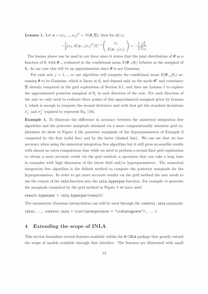
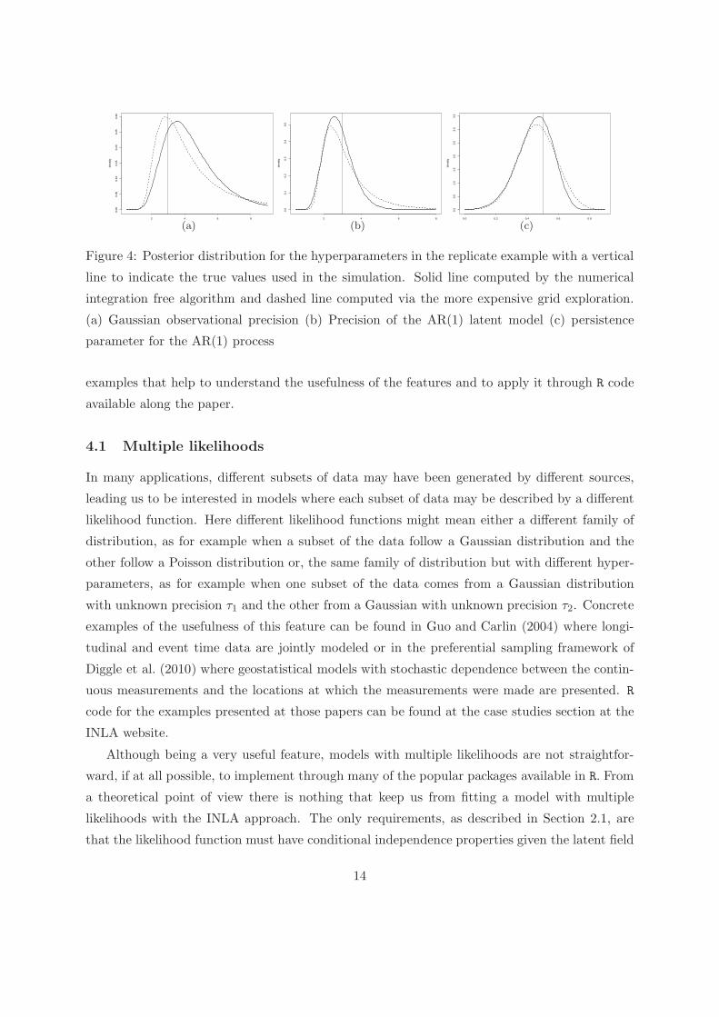
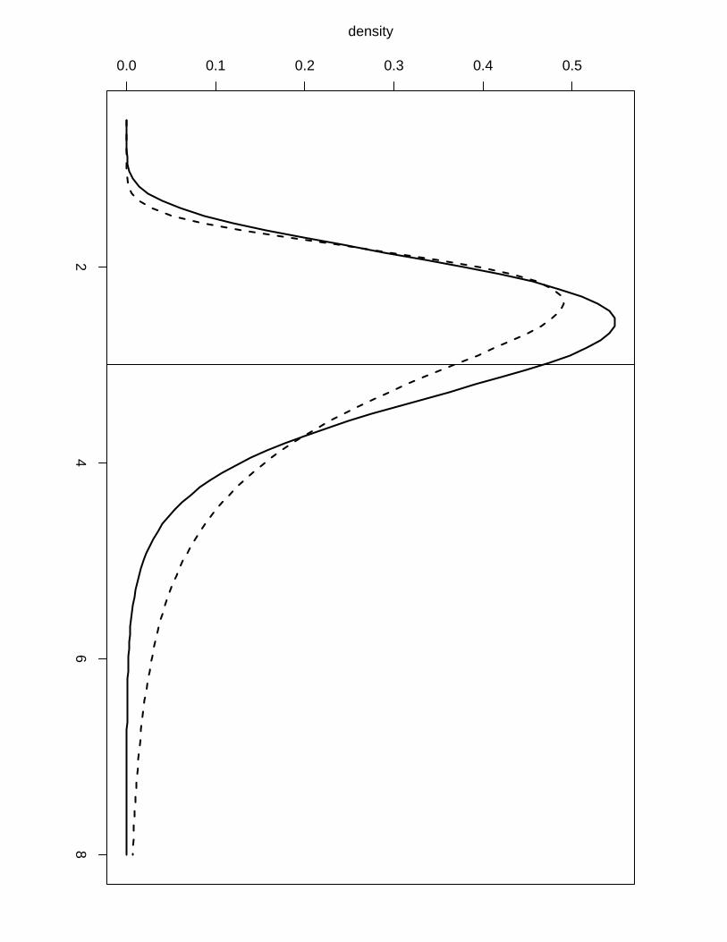
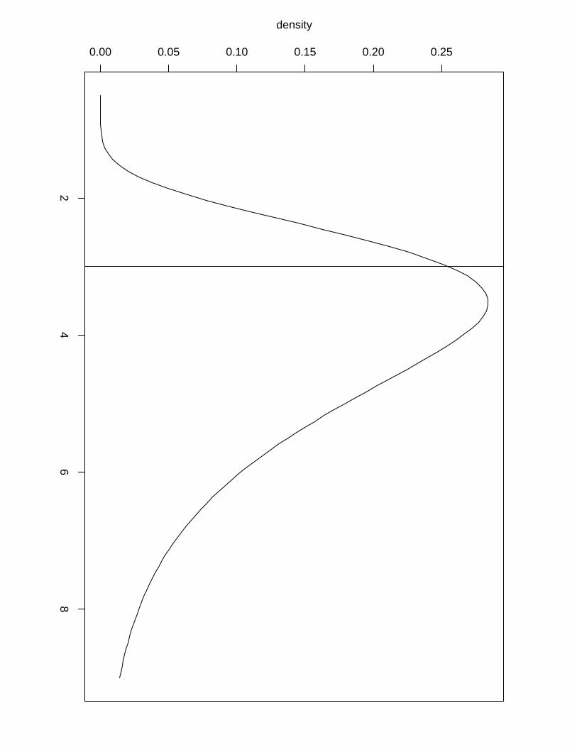
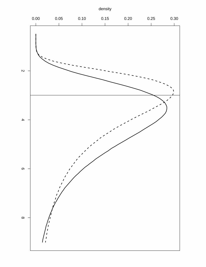
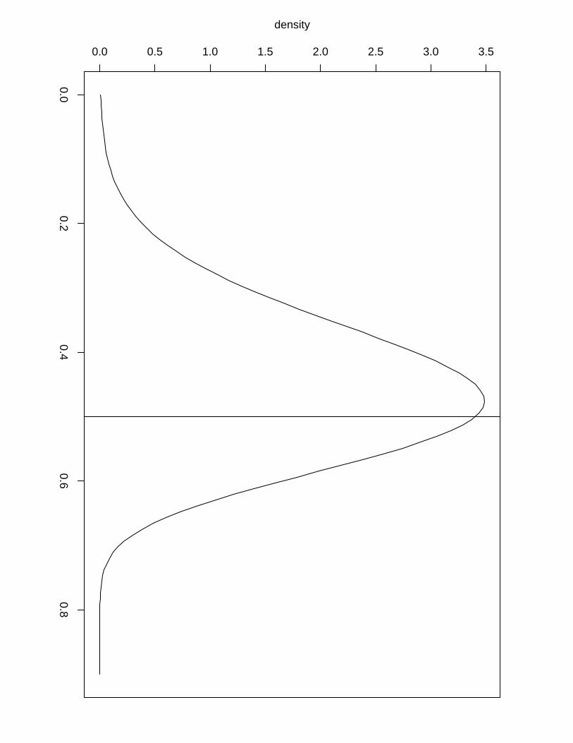
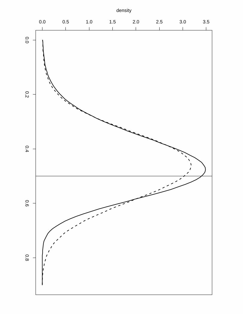
Example 1. To illustrate the difference in accuracy between the numerical integration free

algorithm and the posterior marginals obtained via a more computationally intensive grid ex-

ploration we show in Figure 4 the posterior marginals of the hyperparameters of Example 3

computed by the first (solid line) and by the latter (dashed line). We can see that we lose

accuracy when using the numerical integration free algorithm but it still gives us sensible results

with almost no extra computation time while we need to perform a second finer grid exploration

to obtain a more accurate result via the grid method, a operation that can take a long time

in examples with high dimension of the latent field and/or hyperparameters. The numerical

integration free algorithm is the default method to compute the posterior marginals for the

hyperparameters. In order to get more accurate results via the grid method the user needs to

use the output of the inla function into the inla.hyperpar function. For example, to generate

the marginals computed by the grid method in Figure 4 we have used

result.hyperpar = inla.hyperpar(result)

The asymmetric Gaussian interpolation can still be used through the control.inla argument:

inla(..., control.inla = list(interpolator = "ccdintegrate"), ...)

4 Extending the scope of INLA

This section formalizes several features available within the R-INLA package that greatly extend

the scope of models available through that interface. The features are illustrated with small

13

2 4 6 8

0.00

0.05

0.10

0.15

0.20

0.25

0.30

dens

ity

(a)2 4 6 8

0.0

0.1

0.2

0.3

0.4

0.5

dens

ity

(b)0.0 0.2 0.4 0.6 0.8

0.0

0.5

1.0

1.5

2.0

2.5

3.0

3.5

dens

ity

(c)

Figure 4: Posterior distribution for the hyperparameters in the replicate example with a vertical

line to indicate the true values used in the simulation. Solid line computed by the numerical

integration free algorithm and dashed line computed via the more expensive grid exploration.

(a) Gaussian observational precision (b) Precision of the AR(1) latent model (c) persistence

parameter for the AR(1) process

examples that help to understand the usefulness of the features and to apply it through R code

available along the paper.

4.1 Multiple likelihoods

In many applications, different subsets of data may have been generated by different sources,

leading us to be interested in models where each subset of data may be described by a different

likelihood function. Here different likelihood functions might mean either a different family of

distribution, as for example when a subset of the data follow a Gaussian distribution and the

other follow a Poisson distribution or, the same family of distribution but with different hyper-

parameters, as for example when one subset of the data comes from a Gaussian distribution

with unknown precision τ1 and the other from a Gaussian with unknown precision τ2. Concrete

examples of the usefulness of this feature can be found in Guo and Carlin (2004) where longi-

tudinal and event time data are jointly modeled or in the preferential sampling framework of

Diggle et al. (2010) where geostatistical models with stochastic dependence between the contin-

uous measurements and the locations at which the measurements were made are presented. R

code for the examples presented at those papers can be found at the case studies section at the

INLA website.

Although being a very useful feature, models with multiple likelihoods are not straightfor-

ward, if at all possible, to implement through many of the popular packages available in R. From

a theoretical point of view there is nothing that keep us from fitting a model with multiple

likelihoods with the INLA approach. The only requirements, as described in Section 2.1, are

that the likelihood function must have conditional independence properties given the latent field

14

x and hyperparameters θ1, and that each data-point yi must be connected to one element in

the latent field xi, so that

π(y|x,θ1) =

nd∏

i=1

π(yi|xi,θ1).

Even this last restriction will be made more flexible in Section 4.5 where each data-point yi may

be connected with a linear combination of the elements in the latent field.

Models with multiple likelihoods can be fitted through the R-INLA package by rewriting the

response variable as a matrix (or list) where the number of columns (or elements in the list) are

equal to the number of different likelihood functions. The following small example will help to

illustrate the process.

Example 2. Suppose we have a dataset y with 2n elements where the first n data points come

from a binomial experiment and the last n data points come from a Poisson distribution. In

this case the response variable to be used as input to the inla() function must be written as

a matrix with two columns and 2n rows where the first n elements of the first column hold

the binomial data while the last n elements of the second column hold the Poisson data, and

all other elements of the matrix should be filled with NA. Following is R code to simulate data

following the description above together with R-INLA code to fit the appropriate model to the

simulated data.

n = 100

x1 = runif(n)

eta1 = 1 + x1

y1 = rbinom(n, size = 1, prob = exp(eta1)/(1+exp(eta1))) # binomial data

x2 = runif(n)

eta2 = 1 + x2

y2 = rpois(n, exp(eta2))

Y = matrix(NA, 2*n, 2) # need the response variable as matrix

Y[1:n, 1] = y1 # binomial data

Y[1:n + n, 2] = y2 # poisson data

Ntrials = c(rep(1,n), rep(NA, n)) # required only for binomial data

xx = c(x1, x2)

formula = Y ~ 1 + xx

result = inla(formula, data = list(Y = Y, xx = xx),

family = c("binomial", "poisson"), Ntrials = Ntrials)

summary(result)

plot(result)

15

4.2 Replicate feature

The replicate feature in R-INLA allows us to define models where the latent field x contain

conditional independent replications of the same latent model given some hyperparameters.

Assume for example that z1 and z2 are independent replications from z|θ such that x = (z1,z2)

and

π(x|θ) = π(z1|θ)π(z2|θ) (11)

It is important to note here that although the process z1 and z2 are conditionally independent

given θ they both convey information about θ. A latent model such as (11) can be defined in

the R-INLA package using the replicate argument inside the f() function used to specify the

random effect components as described in Section 2.3.

Example 3. Let us define the following AR(1) process

x1 ∼ N(0, (κ(1 − φ2))−1)

xi = φxi−1 + ǫi; ǫi ∼ N(0, κ−1), i = 2, ..., n

with φ and κ being unknown hyperparameters satisfying |φ| < 1 and κ > 0. Denote by τ the

marginal precision of the process, τ = κ(1 − φ2). Now assume two conditionally independent

realizations z1 and z2 of the AR(1) process defined above given the hyperparameters θ = (φ, τ).

We are then given a dataset y with 2n elements where the first n elements come from a Poisson

with intensity parameters given by exp(z1) and the last n elements of the dataset come from a

Gaussian with mean z2. The latent model x = (z1,z2) described here can be specified with a

two dimensional index (i, r) where i is the position index for each process and r is the index to

label the process. Following is the INLA code to fit the model we just described to simulated

data with φ = 0.5, κ =√2 and Gaussian observational precision τobs = 3. Priors for the

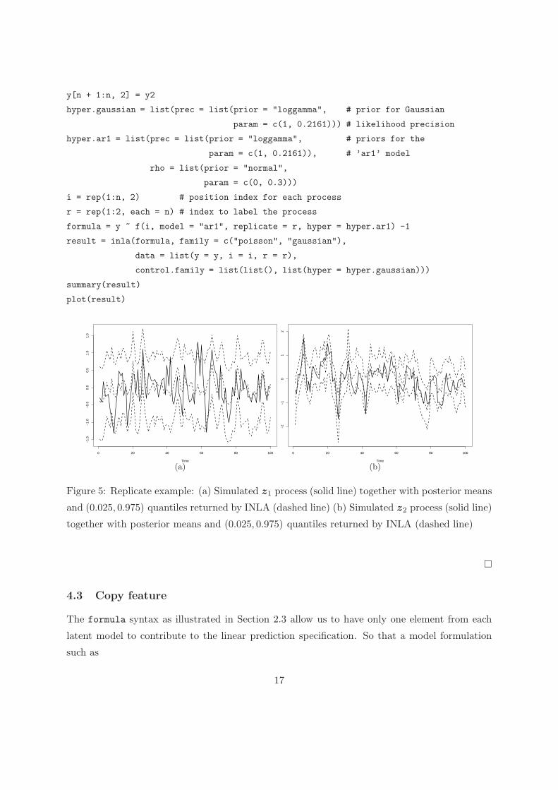
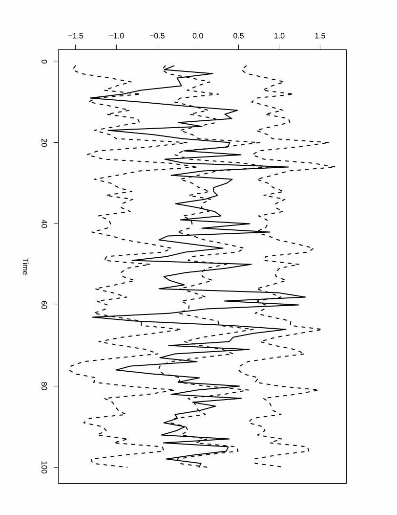
hyperparameters were chosen following the guide-lines described in Fong et al. (2010). Figure

5 show the simulated z = (z1,z2) (solid line) together with posterior means and (0.025, 0.975)-

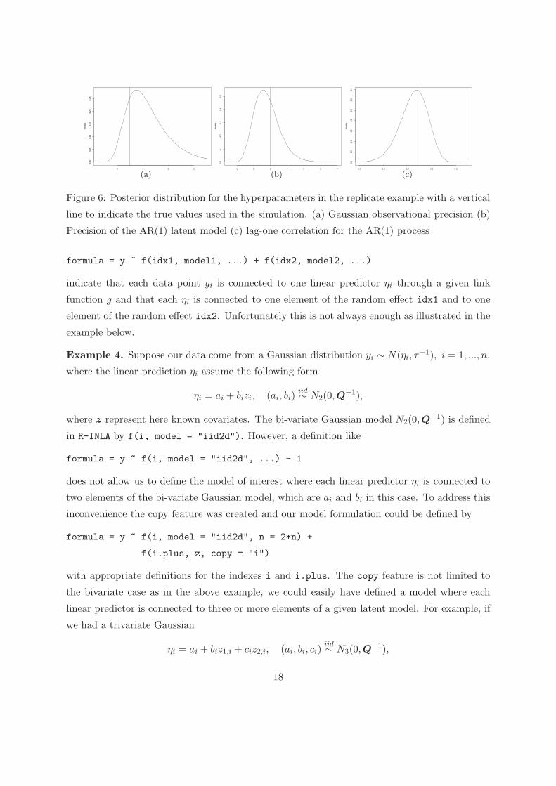
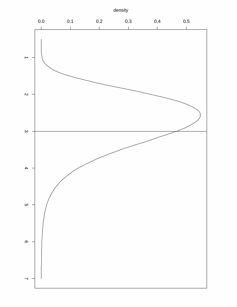
quantiles (dashed line) returned by INLA. Figure 6 show the posterior distributions for the

hyperparameters returned by INLA with a vertical line to indicate true values used in the

simulation.

n = 100

z1 = arima.sim(n, model = list(ar = 0.5), sd = 0.5) # independent replication

z2 = arima.sim(n, model = list(ar = 0.5), sd = 0.5) # from AR(1) process

y1 = rpois(n, exp(z1))

y2 = rnorm(n, mean = z2, sd = 1/sqrt(3))

y = matrix(NA, 2*n, 2) # Setting up matrix due to multiple likelihoods

y[1:n, 1] = y1

16

y[n + 1:n, 2] = y2

hyper.gaussian = list(prec = list(prior = "loggamma", # prior for Gaussian

param = c(1, 0.2161))) # likelihood precision

hyper.ar1 = list(prec = list(prior = "loggamma", # priors for the

param = c(1, 0.2161)), # ’ar1’ model

rho = list(prior = "normal",

param = c(0, 0.3)))

i = rep(1:n, 2) # position index for each process

r = rep(1:2, each = n) # index to label the process

formula = y ~ f(i, model = "ar1", replicate = r, hyper = hyper.ar1) -1

result = inla(formula, family = c("poisson", "gaussian"),

data = list(y = y, i = i, r = r),

control.family = list(list(), list(hyper = hyper.gaussian)))

summary(result)

plot(result)

Time

0 20 40 60 80 100

−1.

5−

1.0

−0.

50.

00.

51.

01.

5

(a)Time

0 20 40 60 80 100

−2

−1

01

2

(b)

Figure 5: Replicate example: (a) Simulated z1 process (solid line) together with posterior means

and (0.025, 0.975) quantiles returned by INLA (dashed line) (b) Simulated z2 process (solid line)

together with posterior means and (0.025, 0.975) quantiles returned by INLA (dashed line)

�

4.3 Copy feature

The formula syntax as illustrated in Section 2.3 allow us to have only one element from each

latent model to contribute to the linear prediction specification. So that a model formulation

such as

17

2 4 6 8

0.00

0.05

0.10

0.15

0.20

0.25

dens

ity

(a)1 2 3 4 5 6 7

0.0

0.1

0.2

0.3

0.4

0.5

dens

ity

(b)0.0 0.2 0.4 0.6 0.8

0.0

0.5

1.0

1.5

2.0

2.5

3.0

3.5

dens

ity

(c)

Figure 6: Posterior distribution for the hyperparameters in the replicate example with a vertical

line to indicate the true values used in the simulation. (a) Gaussian observational precision (b)

Precision of the AR(1) latent model (c) lag-one correlation for the AR(1) process

formula = y ~ f(idx1, model1, ...) + f(idx2, model2, ...)

indicate that each data point yi is connected to one linear predictor ηi through a given link

function g and that each ηi is connected to one element of the random effect idx1 and to one

element of the random effect idx2. Unfortunately this is not always enough as illustrated in the

example below.

Example 4. Suppose our data come from a Gaussian distribution yi ∼ N(ηi, τ−1), i = 1, ..., n,

where the linear prediction ηi assume the following form

ηi = ai + bizi, (ai, bi)iid∼ N2(0,Q

−1),

where z represent here known covariates. The bi-variate Gaussian model N2(0,Q−1) is defined

in R-INLA by f(i, model = "iid2d"). However, a definition like

formula = y ~ f(i, model = "iid2d", ...) - 1

does not allow us to define the model of interest where each linear predictor ηi is connected to

two elements of the bi-variate Gaussian model, which are ai and bi in this case. To address this

inconvenience the copy feature was created and our model formulation could be defined by

formula = y ~ f(i, model = "iid2d", n = 2*n) +

f(i.plus, z, copy = "i")

with appropriate definitions for the indexes i and i.plus. The copy feature is not limited to

the bivariate case as in the above example, we could easily have defined a model where each

linear predictor is connected to three or more elements of a given latent model. For example, if

we had a trivariate Gaussian

ηi = ai + biz1,i + ciz2,i, (ai, bi, ci)iid∼ N3(0,Q

−1),

18

we would use

formula = y ~ f(i, model = "iid3d", n = 3*n) +

f(i.plus1, z1, copy = "i") +

f(i.plus2, z2, copy = "i")

with appropriate definitions for the indexes i, i.plus1 and i.plus2.

Below is R code to simulate data and to fit the bivariate model described above with INLA.

The data is simulated with observational precision τ = 1 and bi-variate Gaussian distribution

for the random-effects (ai, bi), i = 1, ..., 1000 with marginal precisions τa = τb = 1 for ai and

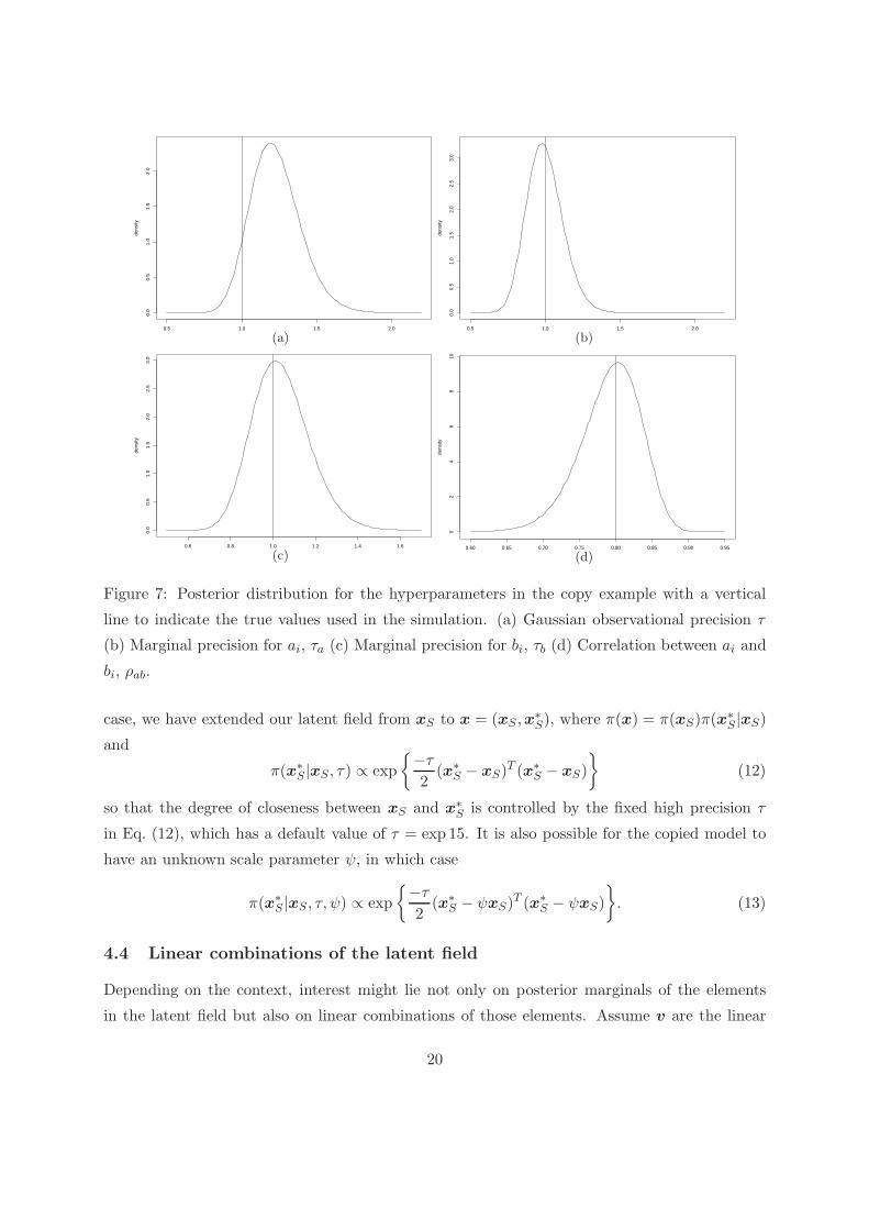
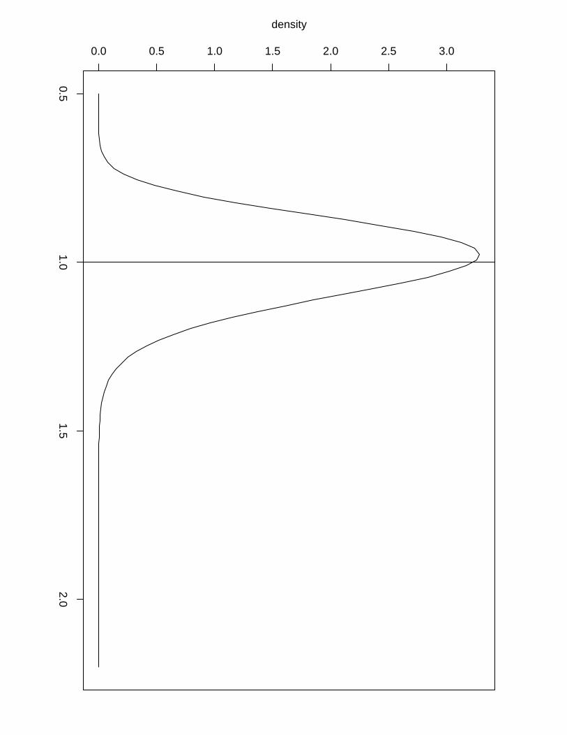
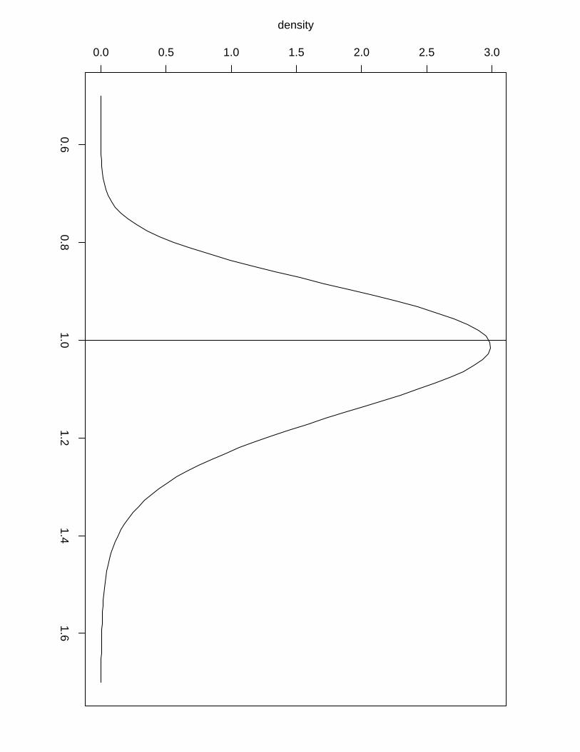
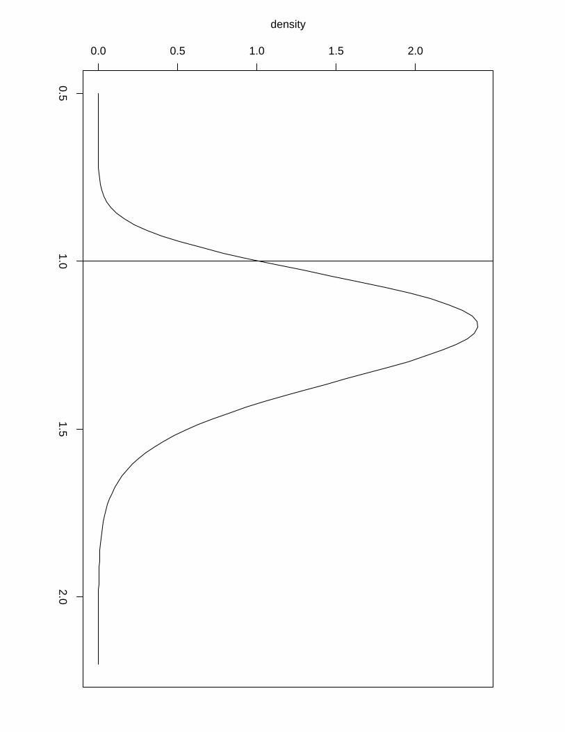
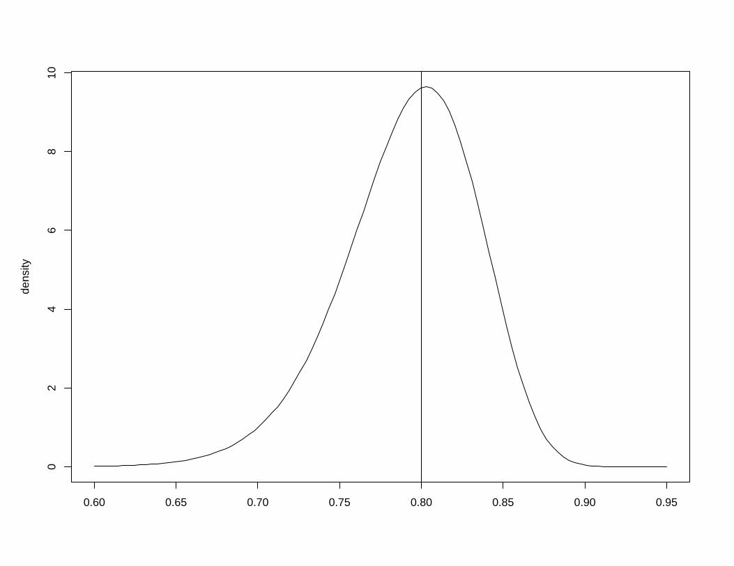
bi respectively, and correlation ρab between ai and bi equal to 0.8. Figure 7 show the posterior

marginals for the hyperparameters returned by INLA.

n = 1000

Sigma = matrix(c(1, 0.8, 0.8, 1), 2, 2)

z = rnorm(n)

ab = rmvnorm(n, sigma = Sigma) # require ’mvtnorm’ package

a = ab[, 1]

b = ab[, 2]

eta = a + b * z

y = eta + rnorm(n, sd = 1)

hyper.gaussian = list(prec = list(prior = "loggamma",

param = c(1, 0.2161)))

i = 1:n # use only the first n elements (a_1, ..., a_n)

j = 1:n + n # use only the last n elements (b_1, ..., b_n)

formula = y ~ f(i, model = "iid2d", n = 2*n) +

f(j, z, copy = "i") - 1

result = inla(formula, data = list(y = y, z = z, i = i, j = j),

family = "gaussian",

control.data = list(hyper = hyper.gaussian))

summary(result)

plot(result)

�

Formally, the copy feature is used when a latent field is needed more than once in the model

formulation. When using the feature we then create a (almost) identical copy of xS, denoted

here by x∗S , that can then be used in the model formulation as shown in Example 4. In this

19

0.5 1.0 1.5 2.0

0.0

0.5

1.0

1.5

2.0

dens

ity

(a)0.5 1.0 1.5 2.0

0.0

0.5

1.0

1.5

2.0

2.5

3.0

dens

ity

(b)

0.6 0.8 1.0 1.2 1.4 1.6

0.0

0.5

1.0

1.5

2.0

2.5

3.0

dens

ity

(c)0.60 0.65 0.70 0.75 0.80 0.85 0.90 0.95

02

46

810

dens

ity

(d)

Figure 7: Posterior distribution for the hyperparameters in the copy example with a vertical

line to indicate the true values used in the simulation. (a) Gaussian observational precision τ

(b) Marginal precision for ai, τa (c) Marginal precision for bi, τb (d) Correlation between ai and

bi, ρab.

case, we have extended our latent field from xS to x = (xS ,x∗S), where π(x) = π(xS)π(x

∗S |xS)

and

π(x∗S |xS , τ) ∝ exp

{−τ2

(x∗S − xS)

T (x∗S − xS)

}(12)

so that the degree of closeness between xS and x∗S is controlled by the fixed high precision τ

in Eq. (12), which has a default value of τ = exp 15. It is also possible for the copied model to

have an unknown scale parameter ψ, in which case

π(x∗S |xS , τ, ψ) ∝ exp

{−τ2

(x∗S − ψxS)

T (x∗S − ψxS)

}. (13)

4.4 Linear combinations of the latent field

Depending on the context, interest might lie not only on posterior marginals of the elements

in the latent field but also on linear combinations of those elements. Assume v are the linear

20

combinations of interest, it can then be written as

v = Bx,

where x is the latent field and B is a k×n matrix where k is the number of linear combinations

and n is the size of the latent field. The functions inla.make.lincomb and inla.make.lincombs

in R-INLA are used to define a linear combination and many linear combinations at once, re-

spectively.

R-INLA provides two approaches for dealing with v. The first approach creates an enlarged

latent field x = (x,v) and then use the INLA method as usual to fit the enlarged model. After

completion we then have posterior marginals for each element of x which includes the linear

combinations v. Using this approach the marginals can be computed using the Gaussian, Laplace

or simplified Laplace approximations discussed in Section 2.2. The drawback is that the addition

of many linear combinations will lead to more dense precision matrices which will consequently

slow down the computations. This approach can be used by defining the linear combinations of

interest using the functions mentioned on the previous paragraph and using control.inla =

list(lincomb.derived.only = FALSE)) as an argument to the inla function.

The second approach does not include v in the latent field but perform a post-processing of

the resulting output given by INLA and approximate v|θ,y by a Gaussian where

Ev|θ,y(v) = Bµ∗ and Varv|θ,y(v) = BQ∗−1BT ,

in which µ∗ is the mean of best marginal approximation used for π(xi|θ,y) (i.e. Gaussian,

Simplified Laplace or Laplace approximation) and Q∗ is the precision matrix of the Gaussian

approximation πG(x|θ,y) used in Eq. (5). Then approximation for the posterior marginals of

v are obtained by integrating θ out in a process similar to Eq. (2). The advantage here is that

the computation of the posterior marginals for v does not affect the graph of the latent field,

leading to a much faster approximation. That is why this is the default method in R-INLA, but

more accurate approximations can be obtained by switching to the first approach, if necessary.

Example 5. Following is R code to compute the posterior marginal of a linear combination

between elements of the AR(1) process of Example 3. More specifically, we are interested in

v1 = 3z1,2 − 5z1,4

v2 = z1,3 + 2z1,5,

where zi,j denote the jth element of the latent model zi as defined in Example 3.

21

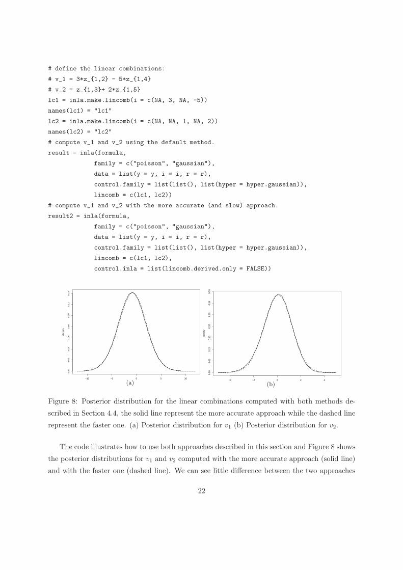
# define the linear combinations:

# v_1 = 3*z_{1,2} - 5*z_{1,4}

# v_2 = z_{1,3}+ 2*z_{1,5}

lc1 = inla.make.lincomb(i = c(NA, 3, NA, -5))

names(lc1) = "lc1"

lc2 = inla.make.lincomb(i = c(NA, NA, 1, NA, 2))

names(lc2) = "lc2"

# compute v_1 and v_2 using the default method.

result = inla(formula,

family = c("poisson", "gaussian"),

data = list(y = y, i = i, r = r),

control.family = list(list(), list(hyper = hyper.gaussian)),

lincomb = c(lc1, lc2))

# compute v_1 and v_2 with the more accurate (and slow) approach.

result2 = inla(formula,

family = c("poisson", "gaussian"),

data = list(y = y, i = i, r = r),

control.family = list(list(), list(hyper = hyper.gaussian)),

lincomb = c(lc1, lc2),

control.inla = list(lincomb.derived.only = FALSE))

−10 −5 0 5 10

0.00

0.02

0.04

0.06

0.08

0.10

0.12

0.14

dens

ity

(a)−4 −2 0 2 4

0.00

0.05

0.10

0.15

0.20

0.25

0.30

0.35

dens

ity

(b)

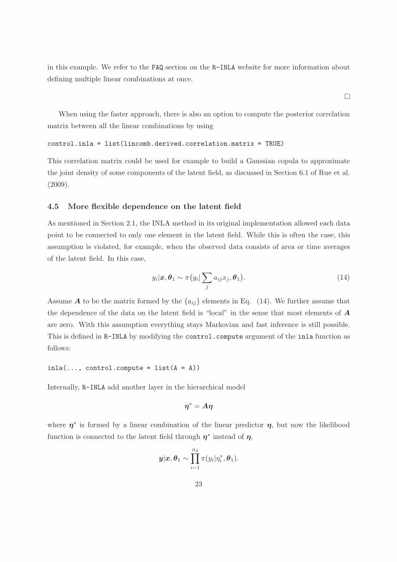
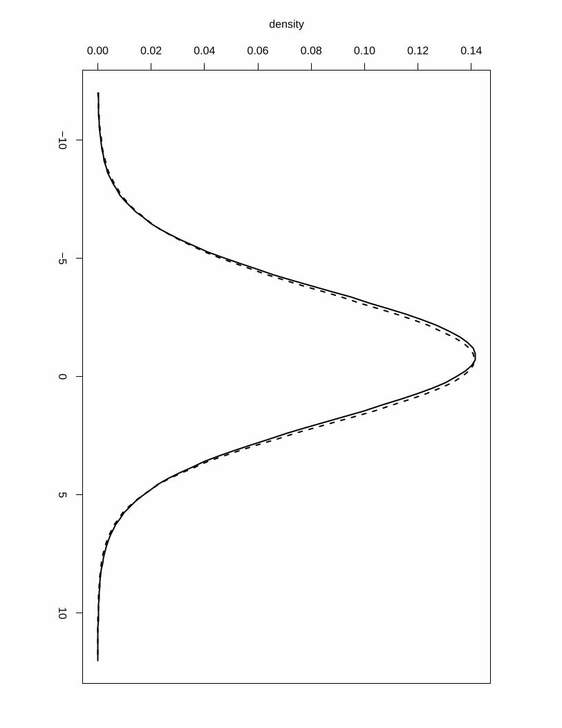
Figure 8: Posterior distribution for the linear combinations computed with both methods de-

scribed in Section 4.4, the solid line represent the more accurate approach while the dashed line

represent the faster one. (a) Posterior distribution for v1 (b) Posterior distribution for v2.

The code illustrates how to use both approaches described in this section and Figure 8 shows

the posterior distributions for v1 and v2 computed with the more accurate approach (solid line)

and with the faster one (dashed line). We can see little difference between the two approaches

22

in this example. We refer to the FAQ section on the R-INLA website for more information about

defining multiple linear combinations at once.

�

When using the faster approach, there is also an option to compute the posterior correlation

matrix between all the linear combinations by using

control.inla = list(lincomb.derived.correlation.matrix = TRUE)

This correlation matrix could be used for example to build a Gaussian copula to approximate

the joint density of some components of the latent field, as discussed in Section 6.1 of Rue et al.

(2009).

4.5 More flexible dependence on the latent field

As mentioned in Section 2.1, the INLA method in its original implementation allowed each data

point to be connected to only one element in the latent field. While this is often the case, this

assumption is violated, for example, when the observed data consists of area or time averages

of the latent field. In this case,

yi|x,θ1 ∼ π(yi|∑

j

aijxj,θ1

). (14)

Assume A to be the matrix formed by the {aij} elements in Eq. (14). We further assume that

the dependence of the data on the latent field is “local” in the sense that most elements of A

are zero. With this assumption everything stays Markovian and fast inference is still possible.

This is defined in R-INLA by modifying the control.compute argument of the inla function as

follows:

inla(..., control.compute = list(A = A))

Internally, R-INLA add another layer in the hierarchical model

η∗ = Aη

where η∗ is formed by a linear combination of the linear predictor η, but now the likelihood

function is connected to the latent field through η∗ instead of η,

y|x,θ1 ∼nd∏

i=1

π(yi|η∗i ,θ1).

23

This is a very powerful feature that allow us to fit models with a likelihood representation given

by Eq. (14) and besides it can even mimic to some extent the copy feature of Section 4.3, with

the exception that the copy feature allow us to copy model components using an unknown scale

parameter as illustrated in Eq. (13). This feature is implemented by also adding η∗ to the latent

model, where the conditional distribution for η∗ has mean Aη and precision matrix κAI where

the constant κA is set to a high value, like κA = exp(15) a priori. In terms of output from inla,

then (η∗,η) is the linear predictor.

To illustrate the relation between the A matrix and the copy feature we fit the model of

Example 4 again but now using the feature described in this Section. Following is the R code:

## This is an alternative implementation of the model in Example 3

i = 1:(2*n)

zz = c(rep(1, n), z)

formula = y ~ f(i, zz, model = "iid2d", n = 2*n) - 1 # Define eta

I = Diagonal(n)

A = cBind(I,I) # Define A matrix used to construct eta* = A eta

result = inla(formula,

data = list(y = y, zz = zz, i = i),

family = "gaussian",

control.predictor = list(A = A))

summary(result)

plot(result)

Although this A-matrix feature can replicate the copy feature to some extent (remember

that copy allow us to copy components with unknown scale parameters), for some models it is

much simpler to use the copy feature. Which one is easier to use varies on a case-by-case basis

and are left to the user to decide which one he or she is most comfortable with.

In some cases it has shown useful to simply define the model using the A-matrix, by simply

defining η as a long vector of all the different components that the full model consist at, and then

putting it all together using the A matrix. The following simplistic linear regression example

demonstrate the idea. Note that η1 is the intercept and η2 is the effect of covariate x.

n = 100

x = rnorm(n)

y = 1 + x + rnorm(n, sd = 0.1)

intercept = c(1, NA)

b = c(NA, 1)

A = cbind(1,x)

r = inla(y ~ -1 + intercept + b, family = "gaussian",

24

data = list(A = A, y = y, intercept = intercept, b = b),

control.predictor = list(A = A))

4.6 Kronecker feature

In a number of applications, the precision matrix in the latent model can be written as a

Kronecker product of two precision matrices. A simple example of this is the separable space-

time model constructed by using spatially correlated innovations in an AR(1) model:

xt+1 = φxt + ǫt,

where φ is a scalar and ǫ ∼ N(0,Q−1ǫ ). In this case the precision matrix is Q = QAR(1) ⊗Qǫ,

where ⊗ is the Kronecker product.

The general Kronecker product mechanism is currently in progress, but a number of special

cases are already available in the code through the group feature. For example, a separable

spatio-temporal model can be constructed using the command

result = y ~ f(loc, model = "besag",

group = time, control.group = list(model = "ar1"))

in which every observation is assigned a location loc and a time time. At each time the points

are spatially correlated while across the time periods, they evolve according to an AR(1) process;

see for example Cameletti et al. (2012). Besides the AR(1) model, an uniform correlation matrix

defining exchangeable latent models, a random-walk of order one (RW1) and of order two (RW2)

are also implemented in R-INLA through the group feature.

5 Conclusion

The INLA framework has become a daily tool for many applied researchers from different areas

of application. With this increase in usage came as well an increase in demand for the possi-

bility to fit more complex models from within R. It has happened in a way that many of the

latest developments have come from necessity expressed by the users. In this paper we have

described and illustrated several new features implemented in the R package R-INLA that have

greatly extended the scope of models available to be used within R. This is an active project

that continues to evolve in order to fulfill, as well as possible, the demands of the statistical and

applied community. Several case studies that have used the features formalized in this paper

can be found in the INLA website. Those case studies treat a variety of situations, as for ex-

ample dynamic models, shared random-effects models, spatio-temporal models and preferential

sampling, and serve to illustrate the generic nature of the features presented in Section 4.

25

Most of the attention in Rue et al. (2009) have been focused on the algorithms to compute

the posterior marginals of the latent field since this is usually the most challenging task given

the usual big size of the latent field. However, the computation of posterior marginals of the

hyperparameters is not straightforward given the high cost to evaluate the approximation to the

joint density of hyperparameters. We have here described two algorithms that have been used

successfully to obtain posterior marginals of the hyperparameters by using the few evaluation

points already computed when integrating out the uncertainty with respect to the hyperparam-

eters in the computation of the posterior marginals of the elements in the latent field.

References

Beale, L., Hodgson, S., Abellan, J., LeFevre, S., and Jarup, L. (2010). Evaluation of spatial

relationships between health and the environment: the rapid inquiry facility. Environmental

health perspectives, 118(9):1306.

Bessell, P., Matthews, L., Smith-Palmer, A., Rotariu, O., Strachan, N., Forbes, K., Cowden, J.,

Reid, S., and Innocent, G. (2010). Geographic determinants of reported human campylobacter

infections in scotland. BMC public health, 10(1):423.

Cameletti, M., Lindgren, F., Simpson, D., and Rue, H. (2012). Spatio-temporal modeling

of particulate matter concentration through the SPDE approach. Advances in Statistical

Analysis, xx(xx):xx–xx. (to appear).

Cseke, B. and Heskes, T. (2011). Approximate marginals in latent gaussian models. Journal of

Machine Learning Research, 12:417–454.

Diggle, P., Menezes, R., and Su, T. (2010). Geostatistical inference under preferential sampling.

Journal of the Royal Statistical Society: Series C (Applied Statistics), 59(2):191–232.

Eidsvik, J., Finley, A., Banerjee, S., and Rue, H. (2011). Approximate bayesian inference

for large spatial datasets using predictive process models. Computational Statistics & Data

Analysis.

Eidsvik, J., Martino, S., and Rue, H. (2009). Approximate bayesian inference in spatial gener-

alized linear mixed models. Scandinavian journal of statistics, 36(1):1–22.

Fong, Y., Rue, H., and Wakefield, J. (2010). Bayesian inference for generalized linear mixed

models. Biostatistics, 11(3):397–412.

26

Guo, X. and Carlin, B. (2004). Separate and joint modeling of longitudinal and event time data

using standard computer packages. The American Statistician, 58(1):16–24.

Haas, S., Hooten, M., Rizzo, D., and Meentemeyer, R. (2011). Forest species diversity reduces

disease risk in a generalist plant pathogen invasion. Ecology letters.

Holand, A., Steinsland, I., Martino, S., and Jensen, H. (2011). Animal models and integrated

nested laplace approximations. Preprint Statistics, (4).

Hosseini, F., Eidsvik, J., and Mohammadzadeh, M. (2011). Approximate bayesian inference in

spatial glmm with skew normal latent variables. Computational Statistics & Data Analysis,

55(4):1791–1806.

Illian, J., Soerbye, S., and Rue, H. (2011). A toolbox for fitting complex spatial point process

models using integrated nested laplace approximation (inla). Annals of Applied Statistics.

Johnson, D., London, J., and Kuhn, C. (2011). Bayesian inference for animal space use and

other movement metrics. Journal of agricultural, biological, and environmental statistics,

16(3):357–370.

Li, Y., Brown, P., Rue, H., al Maini, M., and Fortin, P. (2011). Spatial modelling of lupus

incidence over 40 years with changes in census areas. Journal of the Royal Statistical Society:

Series C (Applied Statistics).

Lindgren, F., Rue, H., and Lindstrom, J. (2011). An explicit link between gaussian fields and

gaussian markov random fields: the stochastic partial differential equation approach. Journal

of the Royal Statistical Society: Series B (Statistical Methodology), 73(4):423–498.

Martino, S., Aas, K., Lindqvist, O., Neef, L., and Rue, H. (2011a). Estimating stochastic

volatility models using integrated nested laplace approximations. The European Journal of

Finance, 17(7):487–503.

Martino, S., Akerkar, R., and Rue, H. (2011b). Approximate bayesian inference for survival

models. Scandinavian Journal of Statistics, 38(3):514–528.

Martins, T. and Rue, H. (2012). Extending INLA to a class of near-Gaussian latent models.

Department of Mathematical Sciences, NTNU, Norway.

Paul, M., Riebler, A., Bachmann, L., Rue, H., and Held, L. (2010). Bayesian bivariate meta-

analysis of diagnostic test studies using integrated nested laplace approximations. Statistics

in medicine, 29(12):1325–1339.

27

Rue, H. and Held, L. (2005). Gaussian Markov random fields: theory and applications. Chapman

& Hall.

Rue, H. and Martino, S. (2007). Approximate Bayesian inference for hierarchical Gaussian

Markov random field models. Journal of statistical planning and inference, 137(10):3177–

3192.

Rue, H., Martino, S., and Chopin, N. (2009). Approximate Bayesian inference for latent Gaussian

models by using integrated nested Laplace approximations. Journal of the Royal Statistical

Society: Series B(Statistical Methodology), 71(2):319–392.

Ruiz-Cardenas, R., Krainski, E., and Rue, H. (2011). Direct fitting of dynamic models using

integrated nested laplace approximations–inla. Computational Statistics & Data Analysis.

Schrodle, B. and Held, L. (2011). Spatio-temporal disease mapping using inla. Environmetrics,

22(6):725–734.

Schrodle, B., Held, L., Riebler, A., and Danuser, J. (2011). Using integrated nested laplace

approximations for the evaluation of veterinary surveillance data from switzerland: a case-

study. Journal of the Royal Statistical Society: Series C (Applied Statistics), 60(2):261–279.

Sørbye, S. and Rue, H. (2010). Simultaneous credible bands for latent gaussian models. Scan-

dinavian Journal of Statistics.

Spiegelhalter, D., Best, N., Carlin, B., and Van Der Linde, A. (2002). Bayesian measures

of model complexity and fit. Journal of the Royal Statistical Society: Series B (Statistical

Methodology), 64(4):583–639.

Tierney, L. and Kadane, J. (1986). Accurate approximations for posterior moments and marginal

densities. Journal of the American Statistical Association, pages 82–86.

Wilking, H., Hohle, M., Velasco, E., Suckau, M., Tim, E., Salinas-Perez, J., Garcia-Alonso, C.,

Molina-Parrilla, C., Jorda-Sampietro, E., Salvador-Carulla, L., et al. (2012). Ecological anal-

ysis of social risk factors for rotavirus infections in berlin, germany, 2007¿ 2009. International

Journal of Health Geographics, 11(1):37.

Wyse, J., Friel, N., and Rue, H. (2011). Approximate simulation-free bayesian inference for

multiple changepoint models with dependence within segments. Bayesian Analysis, 6(4):501–

528.

28

Yue, Y. and Rue, H. (2011). Bayesian inference for additive mixed quantile regression models.

Computational Statistics & Data Analysis, 55(1):84–96.

29

2σ1 0 2σ2

x−

2x

0.51.0

1.52.0

0.0 0.5 1.0 1.5 2.0 2.5 3.0

density

24

68

0.0 0.1 0.2 0.3 0.4 0.5

density

0.60.8

1.01.2

1.41.6

0.0 0.5 1.0 1.5 2.0 2.5 3.0

density

0.51.0

1.52.0

0.0 0.5 1.0 1.5 2.0

density

0.60 0.65 0.70 0.75 0.80 0.85 0.90 0.95

02

46

810

dens

ity

−4

−2

02

4

0.0 0.1 0.2 0.3 0.4

−10

−5

05

10

0.00 0.02 0.04 0.06 0.08 0.10 0.12 0.14

density

12

34

56

7

0.0 0.1 0.2 0.3 0.4 0.5

density

−4

−2

02

4

0.00 0.05 0.10 0.15 0.20 0.25 0.30 0.35

density

24

68

0.00 0.05 0.10 0.15 0.20 0.25

density

24

68

0.00 0.05 0.10 0.15 0.20 0.25 0.30

density

0.00.2

0.40.6

0.8

0.0 0.5 1.0 1.5 2.0 2.5 3.0 3.5

density

0.00.2

0.40.6

0.8

0.0 0.5 1.0 1.5 2.0 2.5 3.0 3.5

density

Tim

e

020

4060

80100

−1.5 −1.0 −0.5 0.0 0.5 1.0 1.5

Time

0 20 40 60 80 100

−2

−1

01

2