Bayesian Vertex Nomination Using Content and...

Advanced Review

Bayesian Vertex Nomination UsingContent and ContextShakira Suwan,1* Dominic S. Lee1 and Carey E. Priebe2

Using attributed graphs to model network data has become an attractive approachfor various graph inference tasks. Consider a network containing a small subset ofinteresting entities whose identities are not fully known and that discovering themwill be of some significance. Vertex nomination, a subclass of recommender systemsrelying on the exploitation of attributed graphs, is a task which seeks to identify theunknown entities that are similarly interesting or exhibit analogous latent attri-butes. This task is a specific type of community detection and is increasingly becom-ing a subject of current research in many disciplines. Recent studies have shownthat information relevant to this task is contained in both the structure of the net-work and its attributes, and that jointly exploiting them can provide superior vertexnomination performance than either one used alone. We adopt this new approachto formulate a Bayesian model for the vertex nomination problem. Specifically, thegoal here is to construct a ‘nomination list’ where entities that are truly interestingare concentrated at the top of the list. Inference with themodel is conducted using aMetropolis-within-Gibbs algorithm. Performance of the model is illustrated by aMonte Carlo simulation study and on the well-known Enron email dataset. © 2015

Wiley Periodicals, Inc.

How to cite this article:WIREs Comput Stat 2015. doi: 10.1002/wics.1365

Keywords: vertex nomination; attributed graphs; stochastic blockmodels; Bayesiananalysis

INTRODUCTION

The representation of data as graphs, with the verti-ces as individuals (articles, people, and neurons)

and the edges as interactions (citations, friendships,synapses) between pairs of vertices, have emerged asa powerful formalism across application domains.The majority of networks often inherently contain arich set of attributes or characteristics attached to eachvertex. For example, in social networks, profile infor-mation of individuals such as names, genders or agescan be encoded as vertex attributes. This type of graph

has been extensively explored in many studies, partic-ularly when information pertaining to a latent classor class membership is embedded with each vertex.Examples include the stochastic blockmodel1 and itsextensions. Similarly, we can have additional informa-tion about the relationship of the vertex pairs, such ascommunication topics and languages, embedded asattributes associated with the edges. Attributedgraphs are becoming increasingly prevalent in networkmodeling for representing a broad variety of databecause their use allows the additional intrinsic infor-mation to be exploited, thereby potentially leading toimproved solutions for various network inferencetasks.

In many disciplines such as neuroscience, biol-ogy, and social science, discovering hidden communitystructures by exploiting information encoded in thegraph topology is often a primary concern. This taskis commonly described as community detection orgraph clustering (see Salter-Townshend et al.2 for a

*Correspondence to: [email protected] of Mathematics and Statistics, University of Canter-bury, Christchurch, New Zealand2Department of Applied Mathematics and Statistics, Johns HopkinsUniversity, Baltimore, MD, USA

Conflict of interest: The authors have declared no conflicts of interestfor this article.

© 2015 Wiley Per iodica ls , Inc.

review of statistical network modeling for communitydetection). Here, community refers to a set of verticesthat display a similar interaction pattern among them-selves compared to the rest of the vertices in the net-work. A special case of this task is the vertexnomination problem. Suppose we have a network con-taining a small subset of interesting entities whose iden-tities are not fully known; in fact, only a few of them areknown. Vertex nomination, introduced by Copper-smith and Priebe3 is a task that seeks to identifythe unknown interesting entities using available vertex-and edge-attribute information, and to do so with aquantifiable measure of being correct. Vertex nomina-tion has connections with the semi-supervised classifi-cation problem in the machine learning literature.

The meaning of ‘interesting’ depends on theapplication context. For example, in the context ofinsider commercial fraud, if the identities of a fewfraudsters are known, law enforcement might wantto find others who may be complicit. Another examplein law enforcement is to identify and prioritize childabuse offenders using the logging of peer-to-peer activ-ities on child pornography networks, motivated by evi-dence of connection between individuals convictedof child pornography possession and child abusers.A country’s national security agency may be interestedin identifying terrorists hidden within the population,starting from the known identities of a few terrorists.Beyond law enforcement and homeland security, ver-tex nomination is also relevant in various social andbusiness contexts; for example, targeted marketingusing recommender systems.4

The most relevant previous works that have animpact on vertex nomination are stochastic blockmo-dels (SBMs)1 and latent position models.5 The SBMassumes that each of n vertices is randomly assignedto one of K blocks, and that the existence of an edgeis independent given the block memberships of a pairof vertices. Furthermore, the probability of an edgedepends only on the blockmemberships of the two ver-tices. The SBM can be considered to be foundationalfor the vertex nomination task. Specifically, in its sim-plest form, the vertex nomination problem can be for-mulated as a two-block SBMwhere one block containsthe interesting vertices and the block membership isobserved for a few of these vertices.6 Proceeding quitein parallel to the development of the SBM, the idea ofmodeling a network by associating a latent positionin a d -dimensional Euclidean space to each vertex gaverise to the latent position model.5 This providedanothermodeling avenue for vertex nomination, whichhas been recently pursued by Sussman et al.7 and Tanget al.8 using spectral embedding techniques and obtain-ing promising results.

Other modeling approaches for the vertex nomi-nation task include Lee et al.9 who developed a multi-variate self-exciting point processmodel that associatesthe memberships of the vertices to the communicationmessaging events on the high risk topic. Marchetteet al.10 extended the random dot product graph modelof Nickel11 and Young and Scheinerman12 a specialcase of the latent positionmodel, by incorporating edgeattributes.When the attribute of interest reflects abnor-mal behavior, vertex nomination can be conceived asan anomaly detection problem and this was pursuedby Priebe et al.13,14 and Grothendieck et al.15 Sunet al.16 made a comparison between graph embeddingmethods for vertex nomination by using a Wilcoxonrank sum test based algorithm to estimate the powerof nominating vertices with a particular attribute ofinterest. For a comprehensive review of vertex nomina-tion, see Coppersmith.17

Recently Fishkind et al.18 proposed several vertexnomination schemes, namely the canonical, spectral-partitioning, and graph-matching vertex nominationschemes, which operate on partially observed unattrib-uted SBM graphs. The canonical method makesuse of the conditional probability of verticesbelonging to the interesting block, given the partiallyobserved graph, to rank the vertices. Unfortunately,prior knowledge of all model parameters are neededto implement this scheme, and it is difficult to computewhen there are more than 20 vertices. It thereforeserves as a comparison benchmark for their otherschemes. The spectral-partitioning scheme uses eigen-decomposition of the adjacency matrix to embed thevertices in a low-dimensional Euclidean space, whichis similar to Tang et al.8 Finally, the graph-matchingscheme utilizes graph-matching tools to construct thenomination list.

Coppersmith and Priebe3 formulated a joint sta-tistical model that operates on an attributed graph,with vertices denoting entities and edges representingcommunications between them. Both vertices andedges have attributes that indicate, respectively,whether an entity or the content of communication isinteresting. By defining context (who communicateswith who) and content (communication topics) statis-tics, and making appropriate assumptions, Copper-smith and Priebe proposed a parametric likelihoodmodel that combined both content and context statis-tics for the vertex nomination task. Even in the simplesttwo-block SBM case, they showed that useful informa-tion for vertex nomination is present in both contentand context, and using both can improve performanceover either one used alone. Therefore, while it is possi-ble to find solutions for vertex nomination using eithercontent or context alone, the use of both is critical for

Advanced Review wires.wiley.com/compstats

© 2015 Wiley Per iodicals , Inc.

achieving optimal performance in real problems. Thismotivates us to further explore the use of both contentand context statistics in a Bayesian perspective.

This paper demonstrates the utility of a Bayesiansolution for the vertex nomination problem, whichjointly exploits information from content and contextstatistics derived from an attributed graph. To facilitatethis, we extend Coppersmith and Priebe’s likelihoodmodel into a Bayesian model by introducing a vectorof latent vertex attributes for the unknown entities,together with appropriate prior distributions for para-meters of the model. Inference with the model is per-formed using a Metropolis-within-Gibbs algorithm,which provides posterior sample points that allow usto estimate the posterior probability that each latentvertex is interesting, and thereafter to obtain a ‘nomi-nation list’. We demonstrate the performance of ourBayesian model using aMonte Carlo simulation study.Another simulation study compares its performanceagainst the method in Coppersmith and Priebe. Anapplication example is provided using the Enron emailcorpus (http://www.enron-mail.com/).

This paper is organized as follows. Details ofthe Bayesian model are described in the next section.The Markov chain Monte Carlo (MCMC) algorithmthat implements the Bayesian solution is givenin Section Inference. Section Simulation Resultsdescribes the simulation studies and the resultsobtained. Experiments using the Enron email corpusare presented in Section Application Results. Finally,Section Conclusion summarizes and concludes thepaper.

MODEL

We proceed by introducing some basic notation beforediscussing specific definitions and models. Consider anunweighted, undirected attributed graph G = (V,E)with no self-loops, multi-edges, or hyper-edges, whereV is the set of vertices with |V| = n, and E is set of edges(i.e., a subset of the set of unordered pairs of vertices).The presence of an edge between two vertices indicatesthat the vertex pair communicates. For the vertexnomination problem, each vertex has an attribute—‘uninteresting’ or ‘interesting’—which is observed fora few vertices but hidden for the rest. Note that whatis hidden are the attributes and not the vertices, i.e.,there are no missing vertices, but most of the vertexattributes are unobserved except for a few ‘interesting’ones. We will refer to a vertex whose attribute is unob-served as a latent vertex. Each edge is also attachedwithan attribute, again ‘uninteresting’ or ‘interesting’,which characterizes the content of the communication.

Here, we assume that all edges and edge attributes areobserved. In what follows, we associate ‘uninteresting’with the color green and the integer 1, and ‘interesting’with the color red and the integer 2. The resulting graphmay thus be represented as an ‘edge-attributed’ adja-cency matrix, A 2 {0, 1, 2}n × n, whose entry Auv = 1 ifthere is a green edge between vertices u and v, Auv = 2if there is a red edge, and Auv = 0 if no edge is present.

Letℳ be the set of red vertices, with |ℳ| =m� n,leaving n −m green vertices inV\ℳ.We assume thatweobserve the vertex attributes of only a few red verticesand none of the green ones. Let ℳ0 �ℳ, with |ℳ0| =m0 > 1, contain those observed red vertices. Thus thelatent vertices whose attributes are unobserved arein V\ℳ0 and there are n −m0 of them (n −m green onesand m −m0 red ones). Put together, we have the con-straints, 1 <m0 ≤m� n. Note that it is possible to haveno latent red vertices.

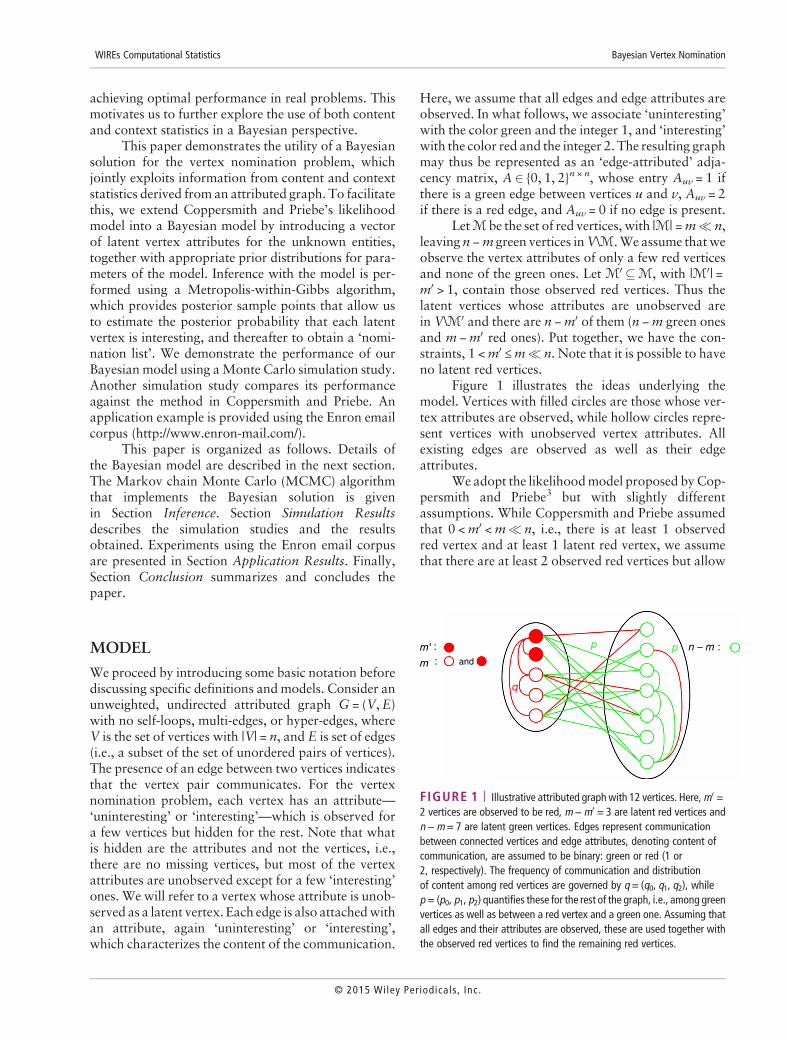
Figure 1 illustrates the ideas underlying themodel. Vertices with filled circles are those whose ver-tex attributes are observed, while hollow circles repre-sent vertices with unobserved vertex attributes. Allexisting edges are observed as well as their edgeattributes.

We adopt the likelihoodmodel proposed byCop-persmith and Priebe3 but with slightly differentassumptions. While Coppersmith and Priebe assumedthat 0 <m0 <m� n, i.e., there is at least 1 observedred vertex and at least 1 latent red vertex, we assumethat there are at least 2 observed red vertices but allow

m' n – m :

m and

q

p p::

FIGURE 1 | Illustrative attributed graph with 12 vertices. Here, m0 =2 vertices are observed to be red, m −m0 = 3 are latent red vertices andn −m= 7 are latent green vertices. Edges represent communicationbetween connected vertices and edge attributes, denoting content ofcommunication, are assumed to be binary: green or red (1 or2, respectively). The frequency of communication and distributionof content among red vertices are governed by q = (q0, q1, q2), whilep = (p0, p1, p2) quantifies these for the rest of the graph, i.e., among greenvertices as well as between a red vertex and a green one. Assuming thatall edges and their attributes are observed, these are used together withthe observed red vertices to find the remaining red vertices.

WIREs Computational Statistics Bayesian Vertex Nomination


http://www.enron-mail.com/

the number of latent red vertices to be 0. These newassumptions remain reasonable for our intended appli-cations. It is plausible that the difference between theirassumptions and ours will have diminishing conse-quence as graph size grows. For the insider commercialfraud example, they translate to having two knownfraudsters who had colluded in the crime and possiblyother (or no other) yet unidentified perpetrators. Moreimportantly, they allow simpler prior distributions thatyield a simplerMCMCalgorithm for implementing ourBayesian solution. If required, switching to Copper-smith and Priebe’s original assumptions can be accom-modated through a different choice of priordistribution that enforces the information that thereis at least 1 latent red vertex. More details about thisare given in the next section.

Let Y(v) be the vertex attribute of vertex v,

Y vð Þ = 1 if vertex is green,2 if vertex is red:

�Wedefine the two statistics asT(v) = (R(v), S(v)), whereR(v) is the number of observed red vertices connectedto v and S(v) is the number of red edges incident to v.These are, respectively, the context and content statis-tics defined in Coppersmith and Priebe and whoshowed that the use of both statistics resulted in bettervertex nomination performance than either one usedalone. The advantage of using both context and contentwas also reported by Qi et al.19 whomodeled multime-dia objects and their user-generated tags as a graphwith context and content links for the purpose of mul-timedia annotation. This is analogous to vertex nomi-nation where the vertices are multimedia objects. Forthe Bayesian approach adopted here, there is potentialto use the number of green edges incident to a vertex asan additional statistic, but at the cost of greater modeland computational complexity. The cost–benefit of thisadded complexity is currently being investigated by theauthors.

For the vertex pair u, v, the edge attributebetween two green vertices or between a green and ared one (i.e., Y(u) =Y(v) = 1 or Y(u) 6¼Y(v)), is con-trolled by the probability vector p = (p0, p1, p2), whileq = (q0, q1, q2) is the probability vector for edge attri-butes between two red vertices (i.e., Y(u) =Y(v) = 2).They can be expressed as follows:

(i) p1 =P Auv = 1jY uð Þ=Y vð Þ= 1ð Þ=P Auv = 1jY uð Þ 6¼Y vð Þð Þ,

p2 =P Auv = 2jY uð Þ=Y vð Þ= 1ð Þ=P Auv = 2jY uð Þ 6¼Y vð Þð Þ;

(ii) q1 =P Auv = 1jY uð Þ =Y vð Þ =2ð Þ,q2 =P Auv = 2jY uð Þ =Y vð Þ =2ð Þ;

where in both cases, p1 and q1 denote the probabilitiesof a green edge, and p2 and q2 denote the probabilities

of a red edge. SinceX2

i = 0pi = 1 and

X2

i =0qi =1, p0

and q0 are the probabilities of having no edge ineach case.

The probability vector q quantify both the fre-quency (q1 + q2) of communication and distribution(q1, q2) of content among red vertices. Likewise,the probability vector p quantify these for the rest ofthe graph, i.e., among green vertices as well as betweena red vertex and a green one—see Figure 1. It is also evi-dent from this figure that the underlying randomgraph is an edge-attributed two-block SBM, with oneblock containing red vertices, and another block con-taining green vertices. Ignoring the edge attributes,the probability of an edge between two red vertices inthis SBM would be q1 + q2. The probability of an edgebetween two green vertices is p1 + p2, which is also theprobability of an edge between a red vertex and agreen one.

Two key assumptions underpinning Copper-smith and Priebe’s model are (1) pairs of red vertices,both observed and latent, communicatewith a differentfrequency from other pairs; and (2) the distribution ofcontent among red vertices is different from the rest ofthe graph. More specifically, it is assumed that p1 = q1and p2 < q2, where the latter prescribes that rededges are more likely between red vertices, and hencea higher frequency of communication among red verti-ces (p1 + p2 < q1 + q2).

The joint distribution of the context andcontent statistics depends on each vertex can bedescribed as follows. Given that a latent greenvertex v 2V\ℳ, the number of observed red verticesconnected to v has a binomial distribution with para-meters m0 and p1 + p2, since there are m0 observed redvertices and these can connect to v via green or rededges; hence,

f1 R vð Þjp1,p2ð Þ =Bin m0,p1 + p2ð Þ; ð1Þ

where Bin(n, p) represents a binomial mass functionwith parameters n and p. The subscript in f1reminds us that this is for a latent green vertex.Likewise, the number of red edges incident to v has abinomial distribution with parameters n − 1 andp2, i.e.,

f1 S vð Þjp2ð Þ =Bin n−1,p2ð Þ: ð2Þ



The joint distribution can be written as

f1 T vð Þjp1,p2ð Þ= f1 S vð ÞjR vð Þ,p1,p2ð Þf1 R vð Þjp1,p2ð Þ= Bin n−m0−1,p2ð Þ*Bin R vð Þ, p2

p1 + p2

� �� Bin m0,p1 + p2ð Þ: ð3Þ

The first term on the RHS is the conditional distribu-tion for the number of red edges incident to v given thatthere are R(v) observed red vertices connected toit. Knowing the number of observed red vertices con-nected to v allows us to partition the number of incidentred edges into those from the connected observed redvertices and those from the other latent vertices. Thedistribution for the number of red edges from the otherlatent vertices is Bin(n −m0 − 1, p2), since there are n −m0 − 1 other latent vertices. The distribution for thenumber of red edges from the connected observedred vertices is Bin(R(v), p2/(p1 + p2)), since the proba-bility that a connecting edge is red is p2/(p1 + p2). Asthese two contributions must sum to S(v), the requiredconditional distribution is a convolution of these twobinomial distributions. Here, g * h denotes the discreteconvolution such that g*h yð Þ =

Xz

g y−zð Þh zð Þ.In a similar way, given a latent red vertex v 2

ℳ\ℳ0 and remembering that q1 = p1, the distributionfor the number of observed red vertices connectedto v is,

f2 R vð Þjp1,q2ð Þ =Bin m0,p1 + q2ð Þ; ð4Þ

where the subscript in f2 indicates that this is for a latentred vertex. The red edges that are incident to v.

f2 S vð Þjm,p2,q2ð Þ =Bin n−m,p2ð Þ*Bin m−1,q2ð Þ; ð5Þ

where S(v) in Eq. (5) can be expressed as the sum of twoindependent discrete variables (i.e., the number of rededges connecting v to latent green vertices and to latentred vertices). Given R(v), S(v) in Eq. (5) can further bedivided. Thus, the double convolution in Eq. (6) of thethree independent discrete random variables, consists ofthe number of red edges connecting v to: (1) the observedred vertices, (2) the latent red vertices, and (3) the latentgreen vertices. Together with Eq. (4), we have

f2 T vð Þjm,p1,p2,q2ð Þ= f2 S vð ÞjR vð Þ,m,p1,p2,q2ð Þf2 R vð Þjp1,q2ð Þ= Bin n−m,p2ð Þ*Bin m−m0−1,q2

� �*Bin R vð Þ, q2

p1 + q2

� �� Bin m0,p1 + q2

� �: ð6Þ

Note that f * g * h is the double convolution,

where f*g*h xð Þ =Xy

f x−yð ÞXz

g y−zð Þh zð Þ" #

.

Given that v 2ℳ0 is an observed red vertex,

f 0 R vð Þjp1,q2ð Þ=Bin m0−1,p1 + q2ð Þ; ð7Þ

f 0 S vð Þjm,p2,q2ð Þ=Bin n−m,p2ð Þ*Bin m−1,q2ð Þ; ð8Þ

f 0 T vð Þjm,p1,p2,q2ð Þ= f 0 S vð ÞjR vð Þ,m,p1,p2,q2ð Þf 0 R vð Þjp1,q2ð Þ

= Bin n−m,p2ð Þ*Bin m−m0,q2ð Þ*Bin R vð Þ, q2p1 +q2

� �� Bin m0−1,p1 +q2ð Þ: ð9Þ

LetT0 = {T0(1),…, T0(m0)} be the statistics for those ver-tices whose attributes are observed to be red. Similarly,let T = {T(1),…, T(n −m0)} be the statistics for thosevertices whose attributes, Y = {Y(1),…, Y(n −m0)}, areunknown. By making the simplifying assumption thatthe statistics are conditionally independent givenY, p1,p2, and q2, the likelihood function is given by

f T,T0jY,p1,p2,q2� �

=Y

i:Y ið Þ = 1f1 T ið Þjp1,p2ð Þ

Yj:Y jð Þ = 2

f2 T jð Þjm,p1,p2,q2ð Þ

Ym0

k= 1

f 0 T0 kð Þjm,p1,p2,q2ð Þ; ð10Þ

where m=m0 +Xn−m0

i = 1

I 2f g Y ið Þð Þ. The first product con-

tains terms from latent green vertices, the second fromlatent red vertices, and the third from observed redvertices.

By Bayes rule, the posterior distribution for theunknown quantities, Y, p1, p2, and q2, is given by

f Y,p1,p2,q2jT,T0� �/ f T,T0jY,p1,p2,q2

� �f Y,p1,p2,q2ð Þ; ð11Þ

where f(Y, p1, p2, q2) is a prior distribution thatmust bespecified. For our problem, the latent attribute vector,Y, is the quantity of interest while p1, p2, and q2 may beregarded as nuisance parameters.

We assume, for the prior distribution, that Y isindependent of (p1, p2, q2), and choose conditionallyindependent Bernoulli(ψ) distributions for the compo-nents of Y with the hyperparameter, ψ = P(Yi = 2),



chosen to follow a beta distribution with parametersα, β > 0. For (p1, p2, q2), we choose a Dirichlet distribu-tion with parameters α0 = α1 = α2 = 1 for (p1, p2), and auniform distribution for q2 conditional on p1 and p2.To summarize, the prior distributions on the modelparameters Y, p1, p2, q2 are

Yjψ �Yn−m0

i = 1

Bernoulli ψð Þ;

ψ �Beta α,βð Þ;q2jp1,p2 �Uniform p2,1−p1ð Þ;p1,p2ð Þ�Dirichlet α0,α1,α2ð Þ:

Hence, the posterior distribution can now be factor-ized as

f Y,p1,p2,q2,ψ jT,T0� �/ f T,T0jY,p1,p2,q2

� �f Yjψð Þf q2jp1,p2ð Þf p1,p2ð Þf ψ jα,βð Þ:

ð12Þ

It is worth noting that, in addition to using latent attri-butes, Y, our Bayesian model also leverages observededge- and vertex-attributes through the content andcontext statistics contained within T and T0.

INFERENCE

Posterior inference can proceed via Markov ChainMonte Carlo (MCMC) using a Metropolis withinGibbs algorithm. Since the components of Y arebinary, they can be updated sequentially using Gibbssampling as follows. Let Y− i =Y\Y(i) denote the vertexattributes for all but vertex i and let γi be the conditionalposterior probability that the latent vertex i is red givenY− i. Thus,

See Appendix A for details.The conditional posterior density of ψ given

Y and nuisance parameters (p1, p2, q2) is

f ψ j T,T0,Y,p1,p2,q2� �

/ψm−m0 + α−1 1−ψð Þn−m + β−1I 0,1ð Þ ψð Þ; ð14Þ

which is the beta(m −m0 + α, n −m + β) density. Thus,ψ can easily be updated using a Gibbs update step.Unfortunately, the conditional posterior distributionof (p1, p2, q2) given Y and ψ does not have a standardform that we can generate from exactly. As such,we use random-walk Metropolis-Hastings toupdate each parameter in turn, using the conditionaldistributions, f(p1|p2, q2), f(p2|p1, q2), and f(q2|p1, p2)as the proposal distributions (see Appendix A fordetails).

Let the state at iteration h be denoted by

Y hð Þ,p hð Þ1 ,p hð Þ

2 ,q hð Þ2 ,ψ hð Þ

� , our Metropolis-within-

Gibbs sampler proceeds according to Algorithm 1.The ability to update ψ using a Gibbs step that

generates from a beta distribution is the motivationfor allowing the number of latent red vertices to be0. This makes the independent Bernoulli model a pos-sible choice as prior for Y. Together with the betahyperprior for ψ , we end up with a conjugate condi-tional posterior in Eq. (14) that facilitates the Gibbsstep for updating ψ . With Coppersmith and Priebe’sassumption that the number of latent red vertices isat least 1, however, the specified prior is no longerappropriate. Letting ΣY =Y(1) + � � � + Y(n −m0), a pos-sible alternative is

f Yjψð Þ=0 ΣY = 0,

ψm−m01−ψð Þn−m

1− 1−ψð Þn−m0 ΣY >0;

8<: ð15Þ

which no longer admits a conjugate hyperprior. Updat-ing of ψ will therefore require an additional Metropo-lis-Hastings step within the Gibbs sampler. The cost–benefit of using this alternative prior model is currentlybeing investigated by the authors.

Performance MeasuresSimilar to recommender systems, vertex nomination ispredominantly concerned with a few suggestions(or interesting vertices) instead of a complete classifica-tion of vertices. Choosing an appropriate performance

γi Y− i,p1,p2,q2,ψð Þ=P Y ið Þ = 2jY− i,T,T0,p1,p2,q2,ψ

� �=

f Y ið Þ= 2,Y− i,p1,p2,q2,ψ jT,T0� �f Y ið Þ= 1,Y− i,p1,p2,q2,ψ jT,T0� �

+ f Y ið Þ = 2,Y− i,p1,p2,q2,ψ jT,T0� � : ð13Þ



measure for vertex nomination depends on the exploi-tation task at hand. Two common exploitationtasks are to identity from among the latent vertices(1) as many vertices as possible that are likely to beinteresting, and (2) one vertex that is most likely tobe interesting. The first task seeks to position as manytruly interesting vertices as possible near the top of aranked nomination list. A performance measure thatis suitable for quantifying this is mean average preci-sion (MAP).3 Average precision (AP) evaluates the pre-cision, at each rank, of the positions of all trulyinteresting vertices in a ranked list, and then averagesthe precision values at the rank of each vertex that istruly interesting.

Let v 1ð Þ,v 2ð Þ,…,v n−m0ð Þ be the ordered latent ver-tices in a ranked list. Following Coppersmith andPriebe3 we define precision at rank r as

π rð Þ=

Xr

i =1

I 2f g Y v ið Þ� ��

r; ð16Þ

and taking the average of the precision values obtainedfrom Eq. (16) as

�π =

Xn−m0

i = 1

I 2f g Y v ið Þ� ��

π ið Þ

m−m0 : ð17Þ



The MAP for a random experiment is defined as

MAP=E �π½ �: ð18Þ

Note that the closer MAP is to 1 the better the model isable to position truly interesting vertices near the top ofa ranked nomination list.

When the exploitation task is to find only oneinteresting vertex, an appropriate measure is the prob-ability of correct nomination, which focuses on gettinga correct result at the top of the nomination list:

Pr v 1ð Þ 2ℳ j ℳ0� �=E I 2f g Y v 1ð Þ

� �� : ð19Þ

The reader is referred to Coppersmith and Priebe3 andManning et al.20 for additional information on theseperformance measures. Here, we will use both MAPand probability of correct nomination to evaluate theperformance of our model.

SIMULATION RESULTS

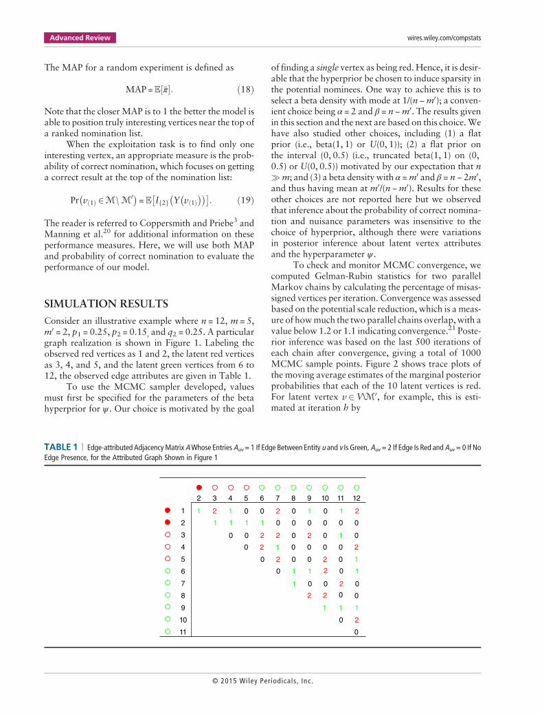
Consider an illustrative example where n = 12, m = 5,m0 = 2, p1 = 0.25, p2 = 0.15, and q2 = 0.25. A particulargraph realization is shown in Figure 1. Labeling theobserved red vertices as 1 and 2, the latent red verticesas 3, 4, and 5, and the latent green vertices from 6 to12, the observed edge attributes are given in Table 1.

To use the MCMC sampler developed, valuesmust first be specified for the parameters of the betahyperprior for ψ . Our choice is motivated by the goal

of finding a single vertex as being red. Hence, it is desir-able that the hyperprior be chosen to induce sparsity inthe potential nominees. One way to achieve this is toselect a beta density with mode at 1/(n −m0); a conven-ient choice being α = 2 and β = n −m0. The results givenin this section and the next are based on this choice.Wehave also studied other choices, including (1) a flatprior (i.e., beta(1, 1) or U(0, 1)); (2) a flat prior onthe interval (0, 0.5) (i.e., truncated beta(1, 1) on (0,0.5) or U(0, 0.5)) motivated by our expectation that n�m; and (3) a beta density with α =m0 and β = n − 2m0,and thus having mean at m0/(n −m0). Results for theseother choices are not reported here but we observedthat inference about the probability of correct nomina-tion and nuisance parameters was insensitive to thechoice of hyperprior, although there were variationsin posterior inference about latent vertex attributesand the hyperparameter ψ .

To check and monitor MCMC convergence, wecomputed Gelman-Rubin statistics for two parallelMarkov chains by calculating the percentage of misas-signed vertices per iteration. Convergence was assessedbased on the potential scale reduction, which is a meas-ure of howmuch the two parallel chains overlap, with avalue below 1.2 or 1.1 indicating convergence.21 Poste-rior inference was based on the last 500 iterations ofeach chain after convergence, giving a total of 1000MCMC sample points. Figure 2 shows trace plots ofthe moving average estimates of the marginal posteriorprobabilities that each of the 10 latent vertices is red.For latent vertex v 2V\ℳ0, for example, this is esti-mated at iteration h by

TABLE 1 | Edge-attributed Adjacency Matrix AWhose Entries Auv = 1 If Edge Between Entity u and v Is Green, Auv = 2 If Edge Is Red and Auv = 0 If NoEdge Presence, for the Attributed Graph Shown in Figure 1

1 0 0

0 0 0 0 0 0

00000

0 0 0 0 0

0000

0 0

0 0 0

00

0

0

0 0

2

2

1

1 1 1 1

1

2 2

2

2

2 2

2

2

2 2

2

2

2 2

21 1 1

1

1

1

1

1 1 1

1 1

3 4 5 6 7 8 9 10 11 12

3

4

5

6

7

8

9

10

11



bPh Y vð Þ= 2jT,T 0ð Þ= 1h

Xhj = 1

I 2f g Y jð Þ vð Þ�

: ð20Þ

Estimates of the marginal posterior probabilitiesthat each of the latent vertices is a red vertex are givenin Table 2. Consequently, vertex number 3, whichhas themaximumprobability, will be posited at the list’sbeginning. In this case, this turns out tobe a correct nom-ination (recall that the latent red vertices are 3, 4, and 5).We advise caution in interpreting these marginal poste-rior probabilities at face values because the relationshipbetween them and the probability of correctnomination is not so straightforward. Again, eventhough we observed that the rankings of these posteriorprobabilities were quite insensitive to the hyperprior forψ , the values of the posterior probabilities do vary withdifferent hyperpriors. Fortunately, we will showlater on that there is evidence of a trend of increasingprobability of correct nomination with increasing max-imum marginal posterior probability of a latent vertexbeing red.

Although inference about the nuisance parametersand hyperparameter is not required, it is interesting tolook at their prior and posterior distributions. The mar-ginal prior and posterior densities are shown in Figure 3.We used a Gaussian kernel density estimator with

diffusion-based bandwidth selection (Algorithm 1 inBotev et al.22).

Figure 3 shows that concentration of the poste-rior densities near the true parameter values, indicatedby red points on the horizontal axis, is evident for p1and p2 but less so for q2 because of the smaller numberof red vertices.We observed that posterior inference for

0.5

0.4

0.3

0.2

P(Y

(v) =

2 ǀT

,T')

0.1

00 100 200 300 400 500 600

MCMC iteration700 800 900

Vertex

3

4

7

Others

1000

FIGURE 2 | Trace plots of the moving average estimates of the marginal posterior probabilities that each of the latent vertices is red. The top-threeranking vertices (3, 4, and 7) are labeled as shown; the others (5, 6, 12, 9, 11, 10, and 8) are clustered together at the bottom. Recall that the three latentred vertices are 3, 4, and 5, and so we have a correct nomination in this case.

TABLE 2 | Posterior Probabilities That Latent Vertex Is Red for theIllustrative Attributed Graph with 12 Vertices

Vertex Number bP Y vð Þ= 2jT,T 0� �3 0.2080

4 0.1510

5 0.0900

6 0.0900

7 0.1060

8 0.0550

9 0.0830

10 0.0640

11 0.0800

12 0.0890



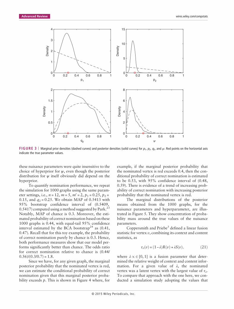
these nuisance parameters were quite insensitive to thechoice of hyperprior for ψ , even though the posteriordistribution for ψ itself obviously did depend on thehyperprior.

To quantify nomination performance, we repeatthe simulation for 1000 graphs using the same param-eter settings, i.e., n = 12, m = 5, m0 = 2, p1 = 0.25, p2 =0.15, and q2 = 0.25. We obtain MAP of 0.5413 with95% bootstrap confidence interval of (0.5409,0.5417) computed using amethod suggested by Park.23

Notably, MAP of chance is 0.3. Moreover, the esti-mated probability of correct nomination based on these1000 graphs is 0.44, with equal-tail 95% confidenceinterval estimated by the BCA bootstrap24 as (0.41,0.47). Recall that for this toy example, the probabilityof correct nomination purely by chance is 0.3. Hence,both performance measures show that our model per-forms significantly better than chance. The odds ratiofor correct nomination relative to chance is (0.44/0.56)/(0.3/0.7) = 1.8.

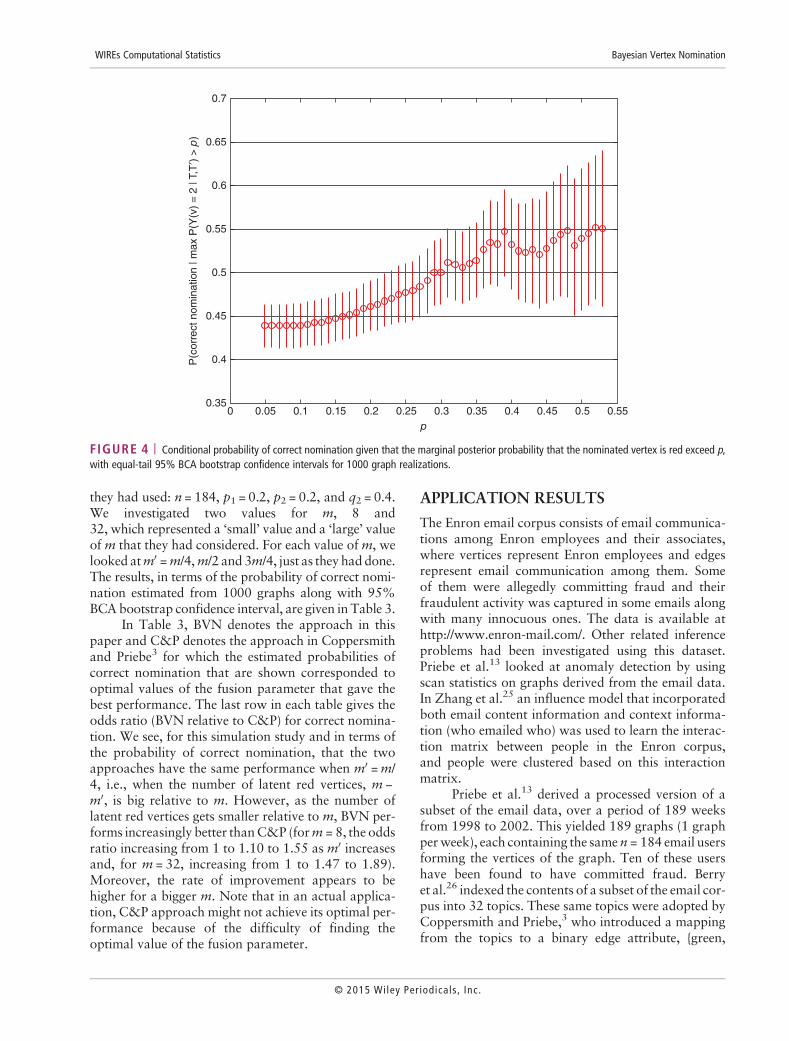
Since we have, for any given graph, the marginalposterior probability that the nominated vertex is red,we can estimate the conditional probability of correctnomination given that this marginal posterior proba-bility exceeds p. This is shown in Figure 4 where, for

example, if the marginal posterior probability thatthe nominated vertex is red exceeds 0.4, then the con-ditional probability of correct nomination is estimatedto be 0.53, with 95% confidence interval of (0.48,0.59). There is evidence of a trend of increasing prob-ability of correct nomination with increasing posteriorprobability that the nominated vertex is red.

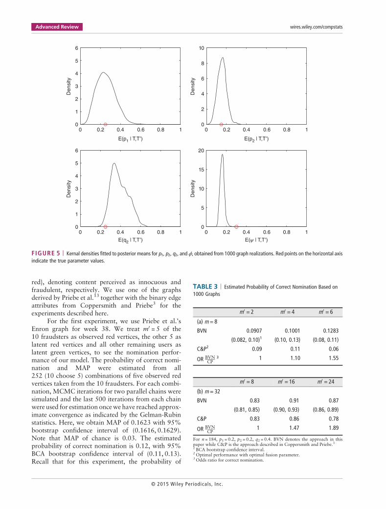
The marginal distributions of the posteriormeans obtained from the 1000 graphs, for thenuisance parameters and hyperparameter, are illus-trated in Figure 5. They show concentration of proba-bility mass around the true values of the nuisanceparameters.

Coppersmith and Priebe3 defined a linear fusionstatistic for vertex v, combining its context and contentstatistics, as

τλ vð Þ = 1−λð ÞR vð Þ+ λS vð Þ; ð21Þ

where λ/2 [0, 1] is a fusion parameter that deter-mined the relative weight of context and content infor-mation. For a given value of λ, the nominatedvertex was a latent vertex with the largest value of τλ.To compare that approach with the one here, we con-ducted a simulation study adopting the values that

p1

0 0.2 0.4 0.6 0.8 1

Den

sity

0

1

2

3

4

q2

0 0.2 0.4 0.6 0.8 1

Den

sity

0

0.5

1

1.5

2

p2

0 0.2 0.4 0.6 0.8 1

Den

sity

0

5

10

15

0 0.2 0.4 0.6 0.8 1

Den

sity

0

2

4

6

8

FIGURE 3 | Marginal prior densities (dashed curves) and posterior densities (solid curves) for p1, p2, q2, and ψ . Red points on the horizontal axisindicate the true parameter values.



they had used: n = 184, p1 = 0.2, p2 = 0.2, and q2 = 0.4.We investigated two values for m, 8 and32, which represented a ‘small’ value and a ‘large’ valueof m that they had considered. For each value ofm, welooked atm0 =m/4,m/2 and 3m/4, just as they haddone.The results, in terms of the probability of correct nomi-nation estimated from 1000 graphs along with 95%BCAbootstrap confidence interval, are given in Table 3.

In Table 3, BVN denotes the approach in thispaper and C&P denotes the approach in Coppersmithand Priebe3 for which the estimated probabilities ofcorrect nomination that are shown corresponded tooptimal values of the fusion parameter that gave thebest performance. The last row in each table gives theodds ratio (BVN relative to C&P) for correct nomina-tion. We see, for this simulation study and in terms ofthe probability of correct nomination, that the twoapproaches have the same performance when m0 =m/4, i.e., when the number of latent red vertices, m −m0, is big relative to m. However, as the number oflatent red vertices gets smaller relative to m, BVN per-forms increasingly better thanC&P (form = 8, the oddsratio increasing from 1 to 1.10 to 1.55 as m0 increasesand, for m = 32, increasing from 1 to 1.47 to 1.89).Moreover, the rate of improvement appears to behigher for a bigger m. Note that in an actual applica-tion, C&P approach might not achieve its optimal per-formance because of the difficulty of finding theoptimal value of the fusion parameter.

APPLICATION RESULTS

The Enron email corpus consists of email communica-tions among Enron employees and their associates,where vertices represent Enron employees and edgesrepresent email communication among them. Someof them were allegedly committing fraud and theirfraudulent activity was captured in some emails alongwith many innocuous ones. The data is available athttp://www.enron-mail.com/. Other related inferenceproblems had been investigated using this dataset.Priebe et al.13 looked at anomaly detection by usingscan statistics on graphs derived from the email data.In Zhang et al.25 an influence model that incorporatedboth email content information and context informa-tion (who emailed who) was used to learn the interac-tion matrix between people in the Enron corpus,and people were clustered based on this interactionmatrix.

Priebe et al.13 derived a processed version of asubset of the email data, over a period of 189 weeksfrom 1998 to 2002. This yielded 189 graphs (1 graphperweek), each containing the same n = 184 email usersforming the vertices of the graph. Ten of these usershave been found to have committed fraud. Berryet al.26 indexed the contents of a subset of the email cor-pus into 32 topics. These same topics were adopted byCoppersmith and Priebe,3 who introduced a mappingfrom the topics to a binary edge attribute, {green,

0.0500.35

0.4

0.45

0.5

P(c

orre

ct n

omin

atio

n | m

ax P

(Y(v

) =

2 |

T,T

′) >

p)

0.55

0.6

0.65

0.7

0.1 0.15 0.2 0.25p

0.3 0.35 0.4 0.45 0.5 0.55

FIGURE 4 | Conditional probability of correct nomination given that the marginal posterior probability that the nominated vertex is red exceed p,with equal-tail 95% BCA bootstrap confidence intervals for 1000 graph realizations.



http://www.enron-mail.com/

red}, denoting content perceived as innocuous andfraudulent, respectively. We use one of the graphsderived by Priebe et al.13 together with the binary edgeattributes from Coppersmith and Priebe3 for theexperiments described here.

For the first experiment, we use Priebe et al.’sEnron graph for week 38. We treat m0 = 5 of the10 fraudsters as observed red vertices, the other 5 aslatent red vertices and all other remaining users aslatent green vertices, to see the nomination perfor-mance of our model. The probability of correct nomi-nation and MAP were estimated from all252 (10 choose 5) combinations of five observed redvertices taken from the 10 fraudsters. For each combi-nation, MCMC iterations for two parallel chains weresimulated and the last 500 iterations from each chainwere used for estimation oncewe have reached approx-imate convergence as indicated by the Gelman-Rubinstatistics. Here, we obtain MAP of 0.1623 with 95%bootstrap confidence interval of (0.1616, 0.1629).Note that MAP of chance is 0.03. The estimatedprobability of correct nomination is 0.12, with 95%BCA bootstrap confidence interval of (0.11, 0.13).Recall that for this experiment, the probability of

TABLE 3 | Estimated Probability of Correct Nomination Based on1000 Graphs

m0 = 2 m0 = 4 m0 = 6

(a) m = 8

BVN 0.0907 0.1001 0.1283

(0.082, 0.10)1 (0.10, 0.13) (0.08, 0.11)

C&P2 0.09 0.11 0.06

OR BVNCP

3 1 1.10 1.55

m0 = 8 m0 = 16 m0 = 24

(b) m = 32

BVN 0.83 0.91 0.87

(0.81, 0.85) (0.90, 0.93) (0.86, 0.89)

C&P 0.83 0.86 0.78

OR BVNCP

1 1.47 1.89

For n = 184, p1 = 0.2, p2 = 0.2, q2 = 0.4. BVN denotes the approach in thispaper while C&P is the approach described in Coppersmith and Priebe.31 BCA bootstrap confidence interval.2Optimal performance with optimal fusion parameter.3Odds ratio for correct nomination.

0.200

1

2

3

4

5

6

0.4

E(p1 | T,T′)

Den

sity

0.6 0.8 1

0.200

1

2

3

4

5

6

0.4

E(q2 | T,T′)

Den

sity

0.6 0.8 1 0.200

5

10

15

20

0.4

E( | T,T′)

Den

sity

0.6 0.8 1

0.200

2

4

6

8

10

0.4

E(p2 | T,T′)

Den

sity

0.6 0.8 1

FIGURE 5 | Kernal densities fitted to posterior means for p1, p2, q2, and ϕ, obtained from 1000 graph realizations. Red points on the horizontal axisindicate the true parameter values.



correct nomination purely by chance is 5/179 ≈ 0.03.This gives an odds ratio of (0.12/0.88)/(0.03/0.97) =4.41, for correct nomination by the Bayesianmodel rel-ative to chance.

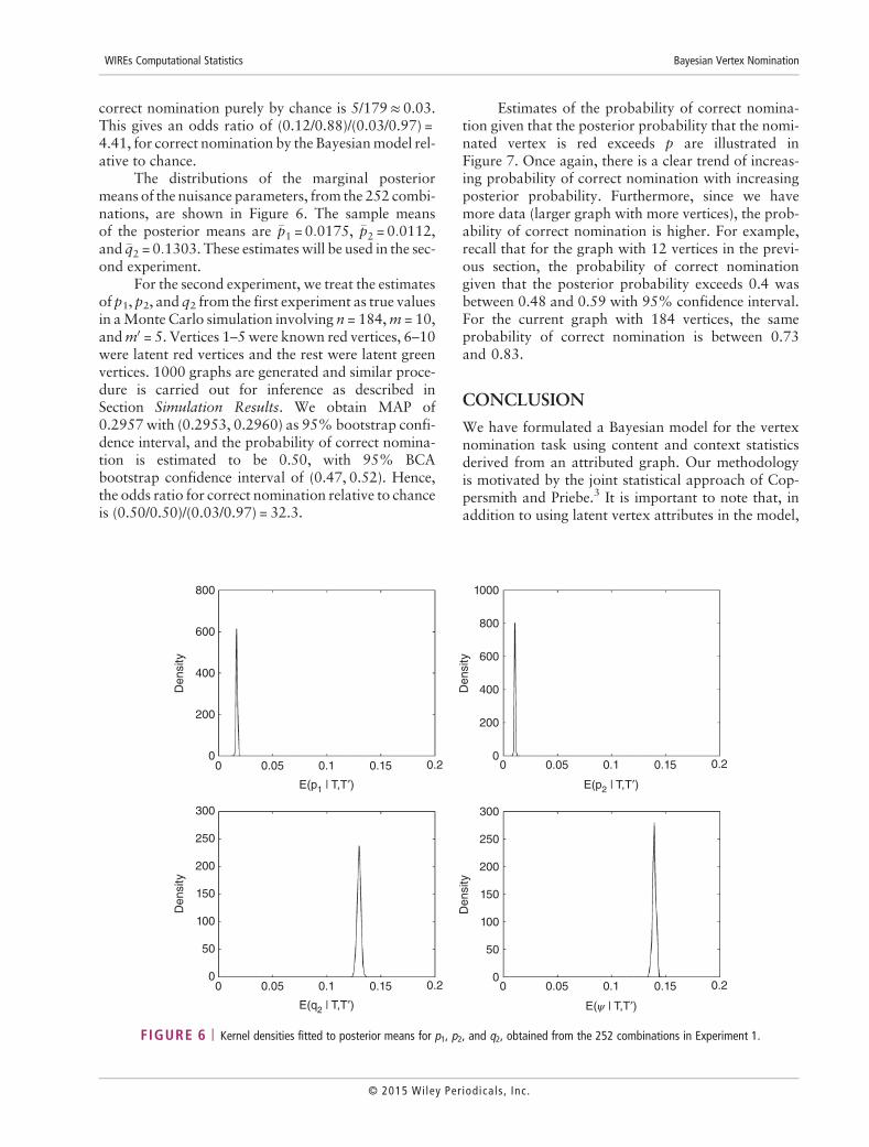
The distributions of the marginal posteriormeans of the nuisance parameters, from the 252 combi-nations, are shown in Figure 6. The sample meansof the posterior means are �p1 = 0:0175, �p2 = 0:0112,and �q2 = 0:1303. These estimates will be used in the sec-ond experiment.

For the second experiment, we treat the estimatesof p1, p2, and q2 from the first experiment as true valuesin aMonte Carlo simulation involving n = 184,m = 10,andm0 = 5. Vertices 1–5were known red vertices, 6–10were latent red vertices and the rest were latent greenvertices. 1000 graphs are generated and similar proce-dure is carried out for inference as described inSection Simulation Results. We obtain MAP of0.2957 with (0.2953, 0.2960) as 95% bootstrap confi-dence interval, and the probability of correct nomina-tion is estimated to be 0.50, with 95% BCAbootstrap confidence interval of (0.47, 0.52). Hence,the odds ratio for correct nomination relative to chanceis (0.50/0.50)/(0.03/0.97) = 32.3.

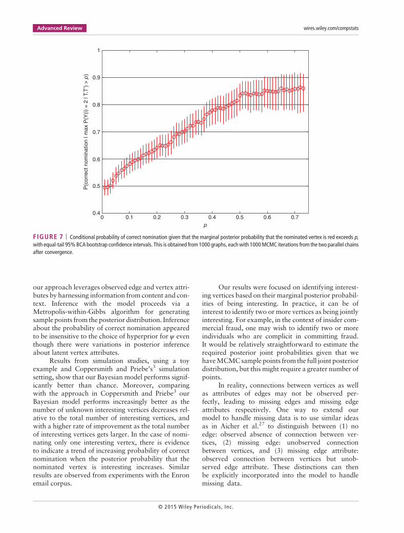
Estimates of the probability of correct nomina-tion given that the posterior probability that the nomi-nated vertex is red exceeds p are illustrated inFigure 7. Once again, there is a clear trend of increas-ing probability of correct nomination with increasingposterior probability. Furthermore, since we havemore data (larger graph with more vertices), the prob-ability of correct nomination is higher. For example,recall that for the graph with 12 vertices in the previ-ous section, the probability of correct nominationgiven that the posterior probability exceeds 0.4 wasbetween 0.48 and 0.59 with 95% confidence interval.For the current graph with 184 vertices, the sameprobability of correct nomination is between 0.73and 0.83.

CONCLUSION

We have formulated a Bayesian model for the vertexnomination task using content and context statisticsderived from an attributed graph. Our methodologyis motivated by the joint statistical approach of Cop-persmith and Priebe.3 It is important to note that, inaddition to using latent vertex attributes in the model,

0.0500

200

400

600

800

0.1

E(p1 | T,T′)

Den

sity

0

200

400

600

800

1000

Den

sity

0.15 0.2

0.0500

100

50

150

200

250

300

0.1

E(q2 | T,T′)

Den

sity

0.15 0.2

0.050 0.1

E(p2 | T,T′)

0.15 0.2

0

50

100

150

200

250

300

Den

sity

0.050 0.1

E( | T,T′)

0.15 0.2

FIGURE 6 | Kernel densities fitted to posterior means for p1, p2, and q2, obtained from the 252 combinations in Experiment 1.



our approach leverages observed edge and vertex attri-butes by harnessing information from content and con-text. Inference with the model proceeds via aMetropolis-within-Gibbs algorithm for generatingsample points from the posterior distribution. Inferenceabout the probability of correct nomination appearedto be insensitive to the choice of hyperprior for ψ eventhough there were variations in posterior inferenceabout latent vertex attributes.

Results from simulation studies, using a toyexample and Coppersmith and Priebe’s3 simulationsetting, show that our Bayesian model performs signif-icantly better than chance. Moreover, comparingwith the approach in Coppersmith and Priebe3 ourBayesian model performs increasingly better as thenumber of unknown interesting vertices decreases rel-ative to the total number of interesting vertices, andwith a higher rate of improvement as the total numberof interesting vertices gets larger. In the case of nomi-nating only one interesting vertex, there is evidenceto indicate a trend of increasing probability of correctnomination when the posterior probability that thenominated vertex is interesting increases. Similarresults are observed from experiments with the Enronemail corpus.

Our results were focused on identifying interest-ing vertices based on their marginal posterior probabil-ities of being interesting. In practice, it can be ofinterest to identify two or more vertices as being jointlyinteresting. For example, in the context of insider com-mercial fraud, one may wish to identify two or moreindividuals who are complicit in committing fraud.It would be relatively straightforward to estimate therequired posterior joint probabilities given that wehaveMCMCsample points from the full joint posteriordistribution, but this might require a greater number ofpoints.

In reality, connections between vertices as wellas attributes of edges may not be observed per-fectly, leading to missing edges and missing edgeattributes respectively. One way to extend ourmodel to handle missing data is to use similar ideasas in Aicher et al.27 to distinguish between (1) noedge: observed absence of connection between ver-tices, (2) missing edge: unobserved connectionbetween vertices, and (3) missing edge attribute:observed connection between vertices but unob-served edge attribute. These distinctions can thenbe explicitly incorporated into the model to handlemissing data.

0.100.4

0.5

0.6

P(c

orre

ct n

omin

atio

n | m

ax P

(Y(i)

= 2

| T,

T′)

> p

)

0.7

0.8

0.9

1

0.2 0.3p

0.4 0.5 0.6 0.7

FIGURE 7 | Conditional probability of correct nomination given that the marginal posterior probability that the nominated vertex is red exceeds p,with equal-tail 95%BCA bootstrap confidence intervals. This is obtained from 1000 graphs, eachwith 1000MCMC iterations from the two parallel chainsafter convergence.



ACKNOWLEDGMENTS

We thank the Review Editor and twoReferees for their comments and useful suggestions. Thanks also to YoungserPark for assisting with the Enron data and for helpful comments on a draft version, and to Celine Cattoen-Gilbertfor suggestions for speeding up computations.

REFERENCES1. Holland PW, Laskey KB, Leinhardt S. Stochastic

blockmodels: first steps. Social Netw 1983,5:109–137.

2. Salter-Townshend M, White A, Gollini I, Murphy T.Review of statistical network analysis: models, algo-rithms, and software. Stat Anal Data Mining 2012,5:243–264.

3. CoppersmithG, Priebe C. Vertex nomination via contentand context. arXiv:1201.4118v1, 2012.

4. Resnick P, Varian H. Recommender systems. CommunACM 1997, 40:56–58.

5. Hoff P, Raftery A, Handcock M. Latent spaceapproaches to social network analysis. J Am Stat Assoc2002, 97:1090–1098.

6. Nowicki K, Snijders T. Estimation and prediction for sto-chastic blockstructures. J Am Stat Assoc 2001,96:1077–1087.

7. Sussman DL, TangM, Priebe CE. Consistent latent posi-tion estimation and vertex classification for random dotproduct graphs. IEEE Trans Pattern Anal Mach Intell2014, 36:48–57.

8. Tang M, Sussman DL, Priebe CE. Universally consistentvertex classification for latent positions graphs.Ann Stat2013, 41:1406–1430.

9. Lee N, Leung T, Priebe C. Random graphs based on self-exciting messaging activities, 2011.

10. Marchette D, Priebe C, Coppersmith G. Vertex nomina-tion via attributed random dot product graphs. In: Pro-ceedings of the 57th ISI World Statistics Congress, Vol.6, 16, 2011.

11. Nickel C. Random dot product graphs: a model forsocial networks. PhD Thesis, Johns Hopkins University,2006.

12. Young S, Scheinerman E. Random dot productgraph models for social networks. Workshop onAlgorithms and Models for the Web-graph, 2007,138–149.

13. Priebe C, Conroy J, Marchette D, Park Y. Scan statisticson enron graphs. Comput Math Organ Theory 2005,11:229–247.

14. Priebe C, Park Y, Marchette D, Conroy J, GrothendieckJ, Gorin A. Statistical inference on attributed randomgraphs: fusion of graph features and content: an experi-ment on time series of enron graphs. Comput Stat DataAnal 2010, 54:1766–1776.

15. Grothendieck J, Priebe C, Gorin A. Statistical inferenceon attributed random graphs: fusion of graph featuresand content. Comput Stat Data Anal 2010,54:1777–1790.

16. Sun M, Tang M, Priebe C. A comparison of graphembedding methods for vertex nomination. In: 201211th International Conference on Machine Learningand Applications (ICMLA), IEEE, Volume 1, 2012,398–403.

17. Coppersmith G. Vertex nomination. WIREs ComputStat 2014, 6:144–153.

18. FishkindDE, Lyzinski V, PaoH, Chen L, Priebe CE. Ver-tex nomination schemes for membership prediction.arXiv preprint arXiv:1312.2638, 2013.

19. Qi G, Aggarwal C, Qi T, Ji H, Huang T. Exploring con-text and content links in social media: a latent spacemethod. IEEE Trans Pattern Anal Mach Intell 2012,34:850–862.

20. Manning CD, Raghavan P, Schütze H. Introduction toInformation Retrieval, vol. 1. Cambridge: CambridgeUniversity Press; 2008.

21. Gelman A, Rubin DB. Inference from iterativesimulation using multiple sequences. Statistical Sci1992, 7:457–472.

22. Botev Z, Grotowski J, Kroese D. Kernel density estima-tion via diffusion. Ann Stat 2010, 38:2916–2957.

23. Park L. Bootstrap confidence intervals for mean averageprecision. In: Proceedings of the Fourth ASEARC Con-ference, 2011, 51–54.

24. Efron B. Better bootstrap confidence intervals. J Am StatAssoc 1987, 82:171–185.

25. Zhang D, Gatica-Perez D, Roy D, Bengio S. Modelinginteractions from email communication. In: 2006 I.E.International Conference on Multimedia and Expo,IEEE, 2006, 2037–2040.

26. BerryMW, BrowneM, Signer B. Topic annotated enronemail data set. Philadelphia: Linguistic Data Consor-tium; 2001.

27. Aicher C, Jacobs AZ, Clauset A. Learning latent blockstructure in weighted networks. J Complex Netw2015, 3:221–248.



APPENDIX A: FULL CONDITIONAL POSTERIOR DISTRIBUTION FOR Y

Continuing from Eq. (13), γi can be computed as follows:

1γi Y− i,p1,p2,q2,ψð Þ= 1+

f Y ið Þ= 1,Y− i,p1,p2,q2,ψ jT,T0ð Þf Y ið Þ= 2,Y− i,p1,p2,q2,ψ jT,T0ð Þ

= 1+

1−ψð Þ=ψ �f1 T ið Þjp1,p2ð ÞY

j:j 6¼i,Y jð Þ = 2f2 T jð Þjm− i,p1,p2,q2ð Þ

Ym0

k =1

f 0ðT0 kð Þjm− i,p1,p2,q2

24 1Af2 T ið Þjm− i + 1,p1,p2,q2ð Þ

Yj:j 6¼i,Y jð Þ =2

f2 T jð Þjm− i + 1,p1,p2,q2ð ÞYm0

k = 1

f 0 T0 kð Þjm− i + 1,p1,p2,q2ð Þ

= 1+

1−ψð Þ=ψ �f1 T ið Þjp1,p2ð ÞY

j:j 6¼i,Y jð Þ = 2f2 S jð ÞjR jð Þ,m− i,p1,p2,q2ð Þ

Ym0

k = 1

f 0ðS0 kð ÞjR0 kð Þ,m− i,p1,p2,q2

24 1Af2 T ið Þjm− i + 1,p1,p2,q2ð Þ

Yj:j 6¼i,Y jð Þ =2

f2 S jð ÞjR jð Þ,m− i + 1,p1,p2,q2ð ÞYm0

k= 1

f 0 S0 kð ÞjR0 kð Þ,m− i + 1,p1,p2,q2ð Þ;

ðA1Þ

where m− i =m0 +Xj:j 6¼i

I 2f g Y jð Þð Þ.

The conditional prior distributions of the nuisance parameters: p1, p2, q2Since the joint prior distribution of the nuisance parameters as described in Section 3 is

f p1,p2,q2ð Þ = f q2jp1,p2ð Þf p1,p2ð Þ=Uniform p2,1−p1ð Þ �Dirichlet α0,α1,α2ð Þ: ðA2Þ

Choosing α0 = α1 = α2 = 1 for the Dirichlet distribution gives

f p1,p2,q2ð Þ = 21−p1−p2

I 0,1ð Þ p1ð ÞI 0,1−p1ð Þ p2ð ÞI p2,1−p1ð Þ q2ð Þ; ðA3Þ

and by choice, we specify

f q2j p1,p2ð Þ =Uniform p2,1−p1ð Þ = 1−p1−p2ð Þ−1I p2,1−p1ð Þ q2ð Þ: ðA4Þ

From Eq. (24), the conditional prior for p1|p2, q2 is

f p1j p2,q2ð Þ/ 1−p1−p2ð Þ−1I 0,1−q2ð Þ p1ð Þ; ðA5Þ

which, for p1 2 (0, 1 − q2), can be written as

f p1j p2,q2ð Þ = 1−p1−p2ð Þ−1log 1−p2ð Þ− log q2−p2ð Þ : ðA6Þ



The corresponding conditional distribution function is

F p1j p2,q2ð Þ= log 1−p2ð Þ− log 1−p1−p2ð Þlog 1−p2ð Þ− log q2−p2ð Þ ; ðA7Þ

and so the conditional inverse distribution function is, for u 2 [0, 1],

F−1 uj p2,q2ð Þ= 1−p2− q2−p2ð Þu1−p2ð Þu−1 : ðA8Þ

This enables us to generate from f(p1|p2, q2) easily by the inverse distribution function method. Similarly,

f p2j p1,q2ð Þ/ 1−p1−p2ð Þ−1I 0,q2ð Þ p2ð Þ; ðA9Þ

and so for p2 2 (0, q2),

f p2j p1,q2ð Þ = 1−p1−p2ð Þ−1log 1−p1ð Þ− log 1−p1−q2ð Þ ðA10Þ

F p2j p1,q2ð Þ= log 1−p1ð Þ− log 1−p1−p2ð Þlog 1−p1ð Þ− log 1−p1−q2ð Þ ; ðA11Þ

and

F−1 uj p1,q2ð Þ =1−p1− 1−p1−q2ð Þu1−p1ð Þu−1 : ðA12Þ



Bayesian Vertex Nomination Using Content and...

Documents

Transcript of Bayesian Vertex Nomination Using Content and...