Bayesian Statistics - University of Washington · Bayesian Statistics Adrian Raftery and Jeff Gill...

Bayesian Statistics

Adrian Raftery and Jeff Gill

One-day course for the American Sociological

Association

August 15, 2002

Bayes Course, ASA Meeting, August 2002 c�

Adrian E. Raftery 2002 1

Outline

1. Bayes’s theorem

2. Bayesian estimation� One parameter case

� Conjugate priors� “Noninformative” priors

� Multiparameter case

� Integrating out parameters� Asymptotic approximations

� When is Bayes useful?� Example: regression in macrosociology

3. Bayesian testing and model selection

� Bayesian testing: Bayes factors

� Bayesian model selection: posterior model

probabilities� Bayesian model averaging: Accounting for model

uncertainty

� Examples

4. Further reading



Purposes of Statistics

� Scientific inference:

– Find causes

– Quantify effects

– Compare competing (causal) theories

� Prediction:

– Policy-making

– Forecasting (e.g. future population, results of

legislation)

– Control of processes

� Decision-making



Standard (frequentist) Statistics

� Estimation is based on finding a good point estimate, and

assessing its performance under repetitions of the

experiment (or survey) that gave rise to the data

� The best point estimate is often the maximum likelihood

estimator.

In large samples, for regular models, this is the most

efficient estimator (i.e. the one with the smallest mean

squared error).

In relatively simple models, the MLE is often the

“obvious” estimator.

For example, for estimating the mean of the normal

distribution, the MLE is just the sample mean.

� For testing one hypothesis against another one within

which it is nested (i.e. of which it is a special case), the

best test is often the likelihood ratio test.

� Standard statistical methods for testing nonnested

models against one another, or for choosing among many

models, are not well developed.



Bayesian Statistics

� Based on the idea of expressing uncertainty about

the (unknown) state of nature in terms of probability.

� You start with a probability distribution reflecting

your current state of knowledge.

When new data become available, you update your

probability distribution in light of the new data.

In a probability framework, there is only one way to

do this: via Bayes’s theorem.

� This solves many of the technical problems of

standard statistics:

nonregular models, testing nonnested models,

choosing among many models.

It also provides a way of incorporating external

information (outside the current data set).



� The key idea is subjective probability.

The current distribution of the state of nature

reflects your opinion.

This has been criticized as non-scientific.

However, it turns out that when there a moderate

amount of evidence, even people who disagree

violently initially end up in substantial agreement,

so long as they follow Bayes’s theorem.

And if there isn’t enough evidence, it’s reasonable

for people who disagreed to start with to go on

disagreeing (although not as much as at first).



Bayes’s Theorem: Notation

Bayes’s theorem relates to the problem of adjudicating

between competing hypotheses given observations.

Suppose�

is an event, i.e. something that either

happens or that doesn’t.

Suppose � �� are other events that form a

partition.

This means that their union is the certain event (i.e. at

least one of them is sure to be the case), and their

intersections are zero. Mathematically:

� � �

� � �

where � is the certain event, and

�� where � is the null event.

� �� can be thought of as competing

hypotheses to explain the event observed,�

.



Bayes’s Theorem

Bayes’s Theorem: In that case, the conditional

probability of � � given�

is

��

��

To calculate �� , we may need a further result, the

Law of Total Probability: The overall, or marginal

probability of the event�

, �� , can be expressed in

terms of the probabilities of � � and the conditional

probabilities of�

given each of the � � ’s, as follows:

��

��



Bayes’s Theorem: An Example

Example 1: An item is produced in 3 different factories,

� � � �� .

The proportions produced in the 3 factories, and the

proportions defective in each, are as follows:

Factory % produced % defective

� � 50 2

� � 30 3

� � 20 4

An item is purchased and found to be defective.

This is event�

.

What is the probability that it was from factory � � ?

First, we find the overall probability of a defective,��

, from the Law of Total Probability:

��

� �� Then, Bayes’s theorem tells us the probability that the



item was from factory � � :��

��

� ��

This makes intuitive sense:

Before we found out that the item was defective, we

knew that the probability it was from factory � � was .50.

Then we found out it was defective.

Factory � � has a lower rate of defectives than the other

two, so finding out that the item was defective made it

less likely to be from factory � � , i.e. to have a

probability lower than .50.

And, indeed, so it is: .37 instead of .50.

Another Version of Bayes’s Theorem:

�� where “ � ” means “proportional to.”

To implement this, we calculate �� for each�

, add them up, and then divide by the sum so that they

add up to 1 (which they have to, because they’re



probabilities of a partition).

Example 1 (ctd):

�� ! "� � � �� # $��# �� &% � �'% � ��(�&)��+*,� � � �� !*-��!*$� � ��. � �� (�&/

Then

��

��10 � � ��32 � � ��34 � ��10 ��

Another way of looking at this is that � � , � � , � � are the

possible states of nature, and that�

is the data. (datum)

We then use the data to decide how likely the different

states of nature are relative to one another.

This is the idea that underlies Bayesian statistics.

�� is the probability of the data given the state of

nature � � .

This is called the likelihood of � � .�� is the probability that it was from � � before we

knew whether or not it was defective, i.e. before we

observed the data.

This is called the prior probability of � � .



�� is called the marginal probability of the data, or, for

reasons we will see later, the integrated likelihood.

�� is called the posterior probability of � � given

�.

The set of posterior probabilities

� ��

is called the posterior distribution of the state of nature.

In Bayesian statistics, all inference is based on the

posterior distribution.



Bayesian Estimation of One

Parameter

Now, we consider the situation where the state of nature

is a parameter to be estimated, denoted by � .

For now, we’ll just consider the case where � is

one-dimensional, i.e. where there’s only one parameter.

An example is the mean of a distribution.

This is like the factories and defectives Example 1, but

with the difference that the possible states of nature

form a contintuum, at least approximately, instead of a

small number of discrete values.

The same basic theory applies, though, with

probabilities replaced by probability densities, and sums

replaced by integrals.

We assume that for each possible value of � , we know

what �� is.

As before, this is called the likelihood.

We also assume that we have a probability density

function (pdf), �� , that tells us the relative probability

of each value of � before observing the data.



As before, this is called the prior distribution.

This can come from prior knowledge.

Often it’s specified roughly so that the prior distribution

covers the range of plausible values and is fairly flat

over that range.

We’ll see that there is a sense in which the precise form

of the prior distribution doesn’t matter too much for

estimation.

We’ll give examples in a bit.

Bayes’s Theorem for Parameter Estimation:

Version 1: The posterior distribution of � given data�

is

given by

��

��

� likelihood � prior

integrated likelihood�

where

�� all values of �

��

is the integrated likelihiood.



Version 2:

��

i.e. � likelihood � prior �This gives the posterior distribution only up to a

multiplicative constant, but often this is enough, and

avoids the difficulty of evaluating the integrated

likelihood (also called the normalizing constant in this

context).



Example: Normal Mean with Known

Variance and One Observation

Example 2: (Box and Tiao 1973): Two physicists, A and

B, are trying to estimate a physical constant, � .

They each have prior views based on their professional

experience, their reading of the literature, and so on.

We will approximate the prior distribution of � by a

normal distribution

� ��

Suppose now that an unbiased method of experimental

measurement is available, and that an observation �

made by this method approximately follows a normal

distribution with mean � , and variance � � , where � � is

known from calibration studies.

Then the likelihood is

� � � ��

Then it can be shown that the posterior distribution of �



given � , �� , is also a normal distribution,

� � � ��

with mean��

� � � � ��

� ��

� � �and variance such that

0��

��

where� � � 0

� ��

and� � � 0

� �� The reciprocal of the variance of a distribution is often

called its precision, because the bigger the variance, the

lower the precision.

Thus � � is the prior precision, and � � is the

observation precision.

The posterior mean �� is a weighted average of the prior

mean � � and the observation � , with the weights being

proportional to the associated precisions.



This is an appealing result.

The posterior precision is the sum of the prior and

observation precisions, reflecting the fact that the two

sources of information are pooled together.



Normal Mean with Multiple

Observations

Now suppose that, instead of one measurement � , we

have � independent measurements with the same

experimental method, � � �� .

Then � � �� are conditionally independent given � .

This means that, if we knew � , knowing the value of � �would tell us nothing about � � , and similarly for any pair

of � � values.

Is this true if we don’t know � ? Why?

� � �� are also said to be exchangeable.

Then the likelihood is got by multiplying up the

likelihoods for the individual � � ’s:

�� It can be shown that this is proportional (as a function

of � ) to a normal distribution with mean �� and standard

deviation ��

� .



Then the posterior distribution is again normal,

� � � ��

with mean��

� � � � ��

� ��

� ��

and variance such that

0��

��

where� � � 0

� ��

and� � � �

� � �Thus the posterior mean is again a weighted average of

the prior mean and the mean of the data.

The weight associated with the mean of the data is

proportional to the number of data points.

The weight associated with the prior remains constant

as the amount of data increases.

Thus, with large samples the prior matters very little.

This is a very general result for Bayesian statistics, and

helps to justify its use.



Inference: Summarizing the

Posterior Distribution

In Bayesian statistics, the posterior distribution is “all

ye know on Earth, and all ye need to know”.

It tells us the probability that the parameter of interest

lies in any interval, given all our current information.

A plot of the posterior density is often useful.

Point Estimation: The search for a point estimate is

meaningless, except in the context of a specific

decision context (and most decisions don’t call for point

estimates).

A numerical value can be useful for saying where the

“center” of the distribution is.

The posterior mode (the most likely value) is the most

intuitive summary.

But often the posterior mean is the most easily

available.

The posterior mode and mean are usually close

together, but not always.

Example: Estimating a hard-to-find population (the



number of homeless, the number of unregistered guns

in America, etc.)

Interval Estimation: The most intuitive interval estimate is

formed by the lower 2.5th percentile and the upper

97.5th percentile of the posterior distribution for a 95%

interval (and similarly for other intervals).

There are other proposals in the Bayesian literature, like

the highest posterior density region, but in my view these

do not have much scientific interest.

Roughly summarizing the posterior distribution: Often, in

practice, the posterior mean and posterior standard

deviation are reported.

These are like the MLE and standard error, and are often

close to them numerically.

Posterior mean�

2 posterior standard deviations is a

rough 95% confidence interval.



Conjugate Priors

In the physical constant example, the prior was normal,

and the posterior was too.

So the data updated the parameters of the prior

distribution, but not its form.

This can be very useful in practical work.

A prior distribution that has this property is called a

conjugate prior.

Often priors of this form are flexible enough to

represent prior knowledge fairly well.

Most priors used in applied Bayesian work are

conjugate.



Examples of Conjugate Priors

Some examples of conjugate priors for one parameter

models:

Model Prior distribution

Normal with known variance Normal (for the mean)

Normal with known mean Gamma (for the variance)

Binomial Beta

Poisson Gamma



“Noninformative” Priors

There have been many efforts to find priors that carry

no information, or “noninformative” priors.

In general, this has turned out to be a modern version of

the Philosopher’s Stone.

There are some very simple problems for which there

are agreed “reference” priors.

One example is the normal mean problem, for which a

flat prior�� 0 �

is often used.

This is an “improper” prior, i.e. it does not integrate up

to 1, because it is constant over the whole real line.

Instead, it integrates up to infinity.

Nevertheless, the resulting posterior distribution is

proper.

When there is more than one parameter, though,

“noninformative” priors turn out to be very informative

about some aspects of the problem, in an unexpected

way.



Improper “noninformative” priors can lead to paradoxes

and strange behavior, and should be used with extreme

caution.

The current trend in applied Bayesian statistical work is

towards informative and, if necessary, spread out but

proper prior distributions.



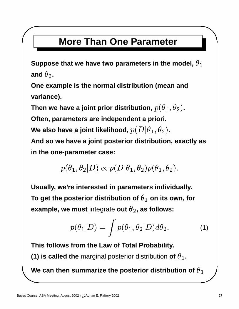
More Than One Parameter

Suppose that we have two parameters in the model, � �and � � .

One example is the normal distribution (mean and

variance).

Then we have a joint prior distribution, �� .Often, parameters are independent a priori.

We also have a joint likelihood, �� .And so we have a joint posterior distribution, exactly as

in the one-parameter case:

��

Usually, we’re interested in parameters individually.

To get the posterior distribution of � � on its own, for

example, we must integrate out � � , as follows:

�� (1)

This follows from the Law of Total Probability.

(1) is called the marginal posterior distribution of � � .We can then summarize the posterior distribution of � �



in the same way as when there’s only one parameter

(posterior mean or mode, posterior standard deviation,

posterior percentiles, plot of the posterior density).

The same approach holds when there are more than two

parameters (e.g. in regression).

Then the integral in (1) is a multiple integral over all the

parameters except � � .



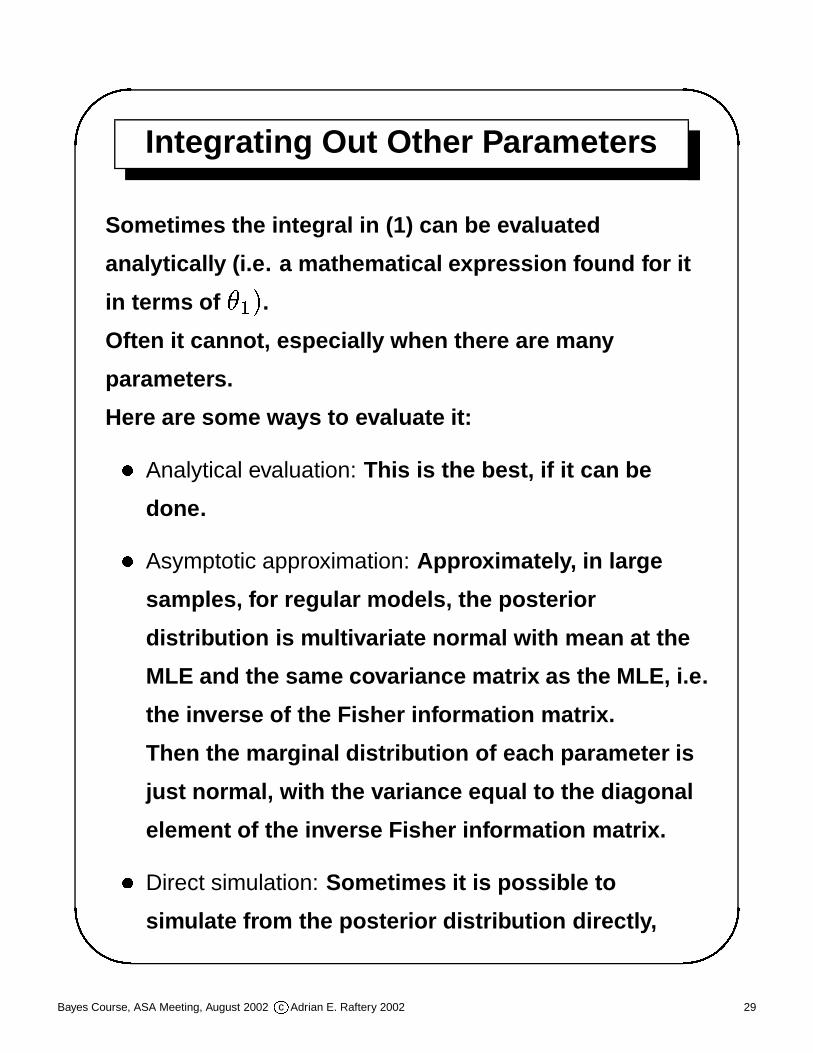
Integrating Out Other Parameters

Sometimes the integral in (1) can be evaluated

analytically (i.e. a mathematical expression found for it

in terms of � � � .Often it cannot, especially when there are many

parameters.

Here are some ways to evaluate it:

� Analytical evaluation: This is the best, if it can be

done.

� Asymptotic approximation: Approximately, in large

samples, for regular models, the posterior

distribution is multivariate normal with mean at the

MLE and the same covariance matrix as the MLE, i.e.

the inverse of the Fisher information matrix.

Then the marginal distribution of each parameter is

just normal, with the variance equal to the diagonal

element of the inverse Fisher information matrix.

� Direct simulation: Sometimes it is possible to

simulate from the posterior distribution directly,



even if it is hard to integrate it out.

Then you can simulate a big sample, and just strip

out the � � values.

This gives you a sample from the marginal posterior

distribution of � � , which can be used to estimate the

posterior mean, standard deviation, percentiles, and

so on.

This is the case in the normal distribution with both

mean and variance unknown.

Then the posterior distribution has the form:

��

� � � �� Gamma �� where � � is the mean and � � is the precision

(reciprocal of the variance).

This can be simulated using an algorithm such as:

Repeat many times:

1. Simulate a value of � � from the gamma

distribution.

This can be done directly using available

software.



2. Simulate a value of � � from the normal

distribution, using the value of � � simulated in

step 1.

� Markov chain Monte Carlo (MCMC) simulation: See Jeff

Gill’s lecture this afternoon.



When is Bayes Better?

We have seen that Bayesian statistics gives very similar

results to standard statistics when three conditions

hold:

1. The model is regular (i.e., roughly, the MLE is

asymptotically normal, which requires, for example,

that the likelihood be smooth and that the amount of

information about each parameter increase as

� ��

),

2. There’s at least a moderate amount of data, and

3. We’re doing estimation, rather than testing or model

selection

Bayesian statistics takes more work in standard

situations, because you have to assess the prior and

investigate sensitivity to it.

Thus, when these 3 conditions hold, Bayesian statistics

involves more work than standard statistics (mostly

MLE and asymptotic standard errors), but yields similar

results.



So it doesn’t seem too worthwhile in this case.

Bayesian statistics can be better in other situations.

� Irregular models: The Bayesian solution is

immediate.

Bayesian statistics doesn’t need regularity

conditions to work.

Examples include: estimating population size;

change-point models; hierarchical models (see

Jeff’s lecture).

� Not much data: Here we can get bad solutions, and

prior information can help a lot.

Examples abound in macrosociology

� Testing and model selection: Here Bayesian

solutions seem more general and avoid many

difficulties with standard methods (nonnested

models, many models, failure to consider power

when setting significance levels.)



Example: Bayesian Inference in

Comparative Research

(Western and Jackman, 1994, APSR)

Problems in comparative research (macrosociology):

� Few cases (e.g. the 23 OECD countries)

� Quite a few parameters in regressions

� Collinearity

� Result: Weak inferences



Example: Explaining Union Density

� Data: 20 democratic countries

� Dependent variable: Union density

� Independent variables: Left government, labor-force

size, economic concentration

� Method: Linear regression



Bayesian Model Selection

� How probable is a model given the data,

conditionally on a set of models

considered, �� ?

� Posterior model probability given data�

:

� � � � � � � � � � �

� Integrated likelihood of a model:

� � � � � � ��

likelihood � prior �

This comes from the law of total probability.



Bayesian Model Selection

(ctd)

Posterior odds for 0 against � :

� � �0��

� � � � 0��

� �0��

where � � � � is the prior probability of� (often taken to be equal),

� Bayes factor ( 0 � ) prior odds



Properties

Theorem 1: For two nested models,

model choice based on the Bayes factor

minimizes the Total Error Rate (= Type I

Error Rate + Type II error rate), on

average over data sets drawn from the

prior.

� Different interpretation of prior:

The set of parameter values over

which we would like good performance

(cf simulation studies).



Bayesian Model Averaging

Suppose is a quantity of interest

which has the same interpretation over

the models considered, e.g. it is an

observable quantity that can be

predicted, at least asymptotically.

Then if there are several models, its

posterior distribution is a weighted

average over the models:

� � � � ��

� � �

� � � ��



Estimation via Bayesian

Model Averaging

� Estimation: The BMA estimate of a

parameter�

is

��

� � �

��

where��

denotes posterior mean

(often � MLE).

� Theorem 2:��

minimises MSE

among point estimators, where MSE is

calculated for data sets drawn from the

prior.



Comments on Bayesian

Model Selection/Averaging

� Deals easily with multiple ( � � ) models

� Deals easily with nonnested models

� For significance tests, a way of choosing

the size of the test to balance power and

significance. Threshold ��

increases slowly with .

� Deals with model uncertainty (datamining)

� Point null hyotheses approximate interval

nulls, so long as the width is less than

about 1/2 standard error (Berger and

Delampady 1987)



The BIC Approximation

� BIC = 2 log maximized likelihood �

no of parameters �� .� Theorem 3:

� �� 0 � � � ��

i.e. BIC approximates the Bayes

factor to within � �� no matter

what the prior is. The � �� term is

unimportant in large samples, so� �� 0 �

, so that BIC is

consistent. (Cox and Hinkley 1978, Schwarz

1978)



The BIC Approximation (ctd)

� Theorem 4: If

� � � � � ��

� � 0 � �

where is the expected information

matrix for one observation, the unit

information prior (UIP), then� �� 0 � � � �� 0 � � �

i.e. the approximation is much

better for the UIP (Kass and Wasserman

1995).

� What if the prior is wrong?

4 slides here: UIP plot, criticism, BF vs prior sd plot, response.



Small Simulation Study

based on Weakliem example.

� Formulate � table as a loglinear model with

ANOVA parametrization

� Keep main effects constant at values in Weakliem

data

� Set log-odds ratio = 0 ( � � ), or LOR �� 0 � ��

( � � ) (Weakliem recommendation)

0 5 10 15 20

0.0

0.1

0.2

0.3

0.4

Simulated Odds Ratios

Odds Ratio

Pro

port

ion

Figure 1:



Tests Assessed

Test

LRT 5%

BIC

BF: default GLIB (scale = 1.65)

BF: right prior



Tests: Total Error Rates

Total error rate = Type I error rate + Type II

error rate

Total Error Rate

Test ( � 1000)

LRT 5% 163

BIC 160

BF: default GLIB 154

BF: right prior 153



Calibration of Tests

Of those data sets for which

��

��

(one star), what

proportion actually had an odds ratio

that was different from 1?

We might hope, somewhere in the

region 95%–99%.

Actually, it was 39%.



Calibration of Bayes Factors

Of those data sets for which the

posterior probability of an association

is between 50% and 95% (weak to

positive evidence), what proportion

actually had an odds ratio that was

different from 1?

We might hope, somewhere in the

region 50%–95%. (Halfway = 73%).

Actually, it was:

BIC: 94%

GLIB default: 71%

GLIB right prior: 73%



When BIC and a 5% Test

Disagree: Is BIC Really Too

Conservative?

� Consider those data sets for which

a 5% test “rejects” independence

(i.e. � � � �� ), but BIC does not

(i.e. � � �� ).

� If BIC were really too conservative,

we would expect association to be

present in most of these cases,

probably not far from 95% of these

cases.

� Actually, it was present in only 48%



of these cases.



Estimators

Estimator

Full model

1. MLE

2. Bayes: GLIB

3. Bayes: right prior

Model selection

4. 5% LRT�

MLE

5. BIC�

MLE

6. Bayes GLIB

7. Bayes right prior

BMA

8. BMA: BIC�

MLE

9. BMA: GLIB

10. BMA: right prior



Estimators: MSEs

Total MSE

Estimator ( � 0 �� )Full model

1. MLE 49

2. Bayes: GLIB 48

3. Bayes: right prior 48

Model selection

4. 5% LRT�

MLE 37

5. BIC�

MLE 35

6. Bayes GLIB 35

7. Bayes right prior 34

BMA

8. BMA: BIC�

MLE 33

9. BMA: GLIB 32

10. BMA: right prior 32



Estimation: Comments

� Overall, BMA � Model selection � Full

model.

� Different trade-offs between MSEs under

the two models.

� Right prior (slightly) � GLIB default �BIC

�MLE � LRT

�MLE � Full model

� Full model less good (MLE and Bayes)

� This can guide choice of “ ” in BIC. E.g. for

event history models, it is better to choose

the number of events than the number of

individuals, or of exposure times.



The Hazelrigg-Garnier Data

Revisited

Australia Belgium France Hungary

292 170 29 497 100 12 2085 1047 74 479 190 14

290 608 37 300 434 7 936 2367 57 1029 2615 347

81 171 175 102 101 129 592 1255 1587 516 3110 3751

Italy Japan Philippines Spain

233 75 10 465 122 21 239 110 76 7622 2124 379

104 291 23 159 258 20 91 292 111 3495 9072 597

71 212 320 285 307 333 317 527 3098 4597 8173 14833

United States West Germany West Malaysia Yugoslavia

1650 641 34 3634 850 270 406 235 144 61 24 7

1618 2692 70 1021 1694 306 176 369 183 37 92 13

694 1648 644 1068 1310 1927 315 578 2311 77 148 223

Denmark Finland Norway Sweden

79 34 2 39 29 2 90 29 5 89 30 0

55 119 8 24 115 10 72 89 11 81 142 3

25 48 84 40 66 79 41 47 47 27 48 29



The Quasi-Symmetry Model

1 4 0

0 2 0

0 0 3

� Accounts for 99.7% of the deviance under

independence.

� Theoretically grounded.

� No easily discernable patterns in the residuals.

� BUT � � � 0 �� on 16 d.f, so � � 0 �� . An

apparently good model is rejected.

� BIC seems to resolve the dilemma: BIC = � ��favors the QS model.

� A more refined analysis using Weakliem’s prior for

parameter 4 gives the same conclusion, with a more

“exact” BIC (from GLIB) = � 2�� . The conclusion is

insensitive to the prior standard deviation.



Further Model Search

� One should continue to search for better

models if the deviance from the BIC-best

model is big enough:

# Model Deviance d.f. BIC

1 Independence 42970 64 42227

2 Quasi-symmetry 150 16 � 36

3 Saturated 0 0 0

4 Explanatory 490 46 � 43

5 Farm asymmetry 26 14 � 137

� Weakliem’s preferred model is # 5, which is

also preferred by BIC, but rejected by a 5%

significance test.



Concluding Remarks

� Bayes factors seem to perform well as tests

(in terms of total error rate). This seems

fairly robust to the prior used. They also

seem well calibrated.

� In the small example considered, Bayes

factors based on “good” priors did better

than BIC, which did better than a 5% LRT.

The GLIB default prior had similar

performance to the optimal.

� For estimation, BMA did better in MSE

terms than model selection estimators,

which did better than estimation for the full

model. These results were robust to the

prior, and BIC did almost as well as more

exact Bayes factors.



Concluding Remarks (ctd)

� When the model doesn’t hold, we can

assess methods using out-of-sample

predictive performance. BMA has

consistently done better than model

selection methods (Bayes or non-Bayes).

(e.g. Volinsky et al 1995)

� It’s important to assess whether any of the

models considered fit the data well.

Diagnostics are useful to suggest better

models, but do not necessarily rule out the

use of a model that is better than others by

Bayes factors.

� Even if a Bayes factor prefers one model to

another, the search for better models

should continue (as in the

Hazelrigg-Garnier example).



Papers and Software

www.stat.washington.edu/raftery� Research� Bayesian Model Selection

BMA Homepage:

www.research.att.com/˜volinsky/bma.html



Further Reading: Books

� Introductory: Peter Lee (1989). Bayesian Statistics: An

Introduction.

� Theory: Jose Bernardo and Adrian Smith (1994).

Bayesian Theory.

� Applied: Andrew Gelman et al (1995). Bayesian Data

Analysis.



Further Reading: Review articles

� Bayesian estimation: W. Edwards, H. Lindeman and

L. Savage (1963). Bayesian statistical inference for

psychological research. Psych. Bull. 70, 193-242.

� Bayesian testing: R. Kass and A. Raftery (1995).

Bayes factors. J. Amer. Statist. Ass. 95, 377–395.

www.stat.washington.edu/tech.reports/tr254.ps

� Bayesian model selection: A. Raftery (1995).

Bayesian model selection in social research (with

discussion). Sociological Methodology 25, 111–195.

www.stat.washington.edu/tech.reports/bic.ps

� Bayesian model averaging: J.A. Hoeting et al (1999).

Bayesian model averaging: A tutorial (with

discussion). Statistical Science 14, 382-417.

www.stat.washington.edu/www/research/online/hoeting1999.pdf



Bayesian Statistics - University of Washington · Bayesian Statistics Adrian Raftery and Jeff Gill...

Documents

Transcript of Bayesian Statistics - University of Washington · Bayesian Statistics Adrian Raftery and Jeff Gill...