Bayesian SEM: A more flexible representation of substantive theory

Bayesian SEM:A more flexible representation of substantive theory

Bengt Muthen & Tihomir Asparouhov

September 29, 2010

1

Abstract

This paper proposes a new approach to factor analysis and structural equation modeling

using Bayesian analysis. The new approach replaces parameter specifications of exact zeros

and exact equalities with approximate zeros and equalities based on informative, small-

variance priors. It is argued that this produces an analysis that better reflects substantive

theories. The proposed Bayesian approach is beneficial in applications where parameters

are added to a conventional model such that a non-identified model is obtained if maximum-

likelihood estimation is applied. This approach is useful for measurement aspects of latent

variable modeling such as with CFA and the measurement part of SEM. Three application

areas are studied: Cross-loadings in CFA, residual correlations in CFA, and measurement

non-invariance in MIMIC modeling. The approach encompasses three elements: Model

testing, model estimation, and model modification. Monte Carlo simulations and real data

are analyzed using Mplus.

2

1 Introduction


using Bayesian analysis. It is argued that current analyses using maximum likelihood (ML)

and likelihood-ratio χ2 testing apply unnecessarily strict models to represent hypotheses

derived from substantive theory. This often leads to rejection of the model (see, e.g., Marsh

et al, 2009) and a series of model modifications that may capitalize on chance (see, e.g.

McCallum, 1992). The hypotheses are reflected in parameters fixed at zero or constrained

to be equal to other parameters. Examples include zero cross-loadings and zero residual

correlations in factor analysis, absence of direct effects from covariates to factor indicators

in structural equation modeling, and multiple-group analysis with measurement invariance.

The new approach is intended to produce an analysis that better reflects substantive

theories. It does so by replacing the parameter specification of exact zeros and exact

equalities with approximate zeros and equalities. The new approach uses Bayesian analysis

to specify informative priors for such parameters. If these parameters were all freed in a

conventional analysis, the model would not be identified. The Bayesian analysis, however,

identifies the model by substantively-driven small-variance priors. Model testing is carried

out using posterior predictive checking which is found to be less sensitive than likelihood-

ratio χ2 testing to ignorable degrees of model misspecification. A side product of the

proposed approach is information to modify the model in line with the use of modification

indices in ML analysis. ML modification indices inform about model improvement when

a single parameter is freed and can lead to a long series of modifications. In contrast, the

proposed approach informs about model modification when all parameters are freed and

does so in a single-step analysis.

Section 2 presents a brief overview of the Bayesian analysis framework that is used.

Sections 4 to 6 present three studies that illustrate the new approach. Each study consists of

a real-data example showing the problem, the proposed Bayesian solution for the real-data

3

problem, and simulations showing how well the method works. Study 1 considers factor

analysis where cross-loadings make simple structure CFA inadequate. As an example, a

re-analysis is made of the classic Holzinger-Swineford mental abilities data, where a simple

structure does not fit well by ML CFA standards. Study 2 considers residual correlations

in factor analysis which make a factor model inadequate. As an example, the big-five

factor model is analyzed using an instrument administered in a British household survey,

where the hypothesized five-factor pattern is not well recovered by ML CFA or EFA due to

many minor factors. Study 3 considers measurement non-invariance in the form of direct

effects from covariates to factor indicators. As an example, responses to an instrument

measuring antisocial behavior are related to demographic variables using a U.S. national

survey, where extensive differential item functioning distorts comparison of factors across

subject groups. All analyses are carried out by Bayesian analysis in Mplus (Muthen &

Muthen, 1998-2010) and scripts are available at www.statmodel.com. Section 7 concludes.

2 Bayesian analysis

Frequentist analysis (e.g., maximum likelihood) and Bayesian analysis differ by the former

viewing parameters as constants and the latter as variables. Maximum likelihood (ML)

finds estimates by maximizing a likelihood computed for the data. Bayes combines prior

distributions for parameters with the data likelihood to form posterior distributions for

the parameter estimates. The priors can be diffuse (non-informative) or informative where

the information may come from previous studies. The posterior provides an estimate in

the form of a mean, median, or mode of the posterior distribution.

There are many books on Bayesian analysis and most are quite technical. Gelman et

al. (2004) provides a good general statistical description, whereas Lynch (2010) gives a

somewhat more introductory account. Press (2003) discusses Bayesian factor analysis. Lee

4

(2007) gives a discussion from a structural equation modeling perspective. Schafer (1997)

gives a statistical discussion from a missing data and multiple imputation perspective,

whereas Enders (2010) gives an applied discussion of these same topics. Statistical overview

articles include Gelfand et al. (1990) and Casella and George (1992). Overview articles of

an applied nature and with a latent variable focus include Scheines et al. (1999), Rupp et

al. (2004), and Yuan and MacKinnon (2009).

Bayesian analysis is firmly established in mainstream statistics and its popularity is

growing. Part of the reason for the increased use of Bayesian analysis is the success of new

computational algorithms referred to as Markov chain Monte Carlo (MCMC) methods.

Outside of statistics, however, applications of Bayesian analysis lag behind. One possible

reason is that Bayesian analysis is perceived as difficult to do, requiring complex statistical

specifications such as those used in the flexible, but technically-oriented general Bayes

program WinBUGS. These observations were the background for developing Bayesian

analysis in Mplus (Muthen & Muthen, 1998-2010). In Mplus, simple analysis specifications

with convenient defaults allow easy access to a rich set of analysis possibilities. Diffuse

priors are used as the default with the possibility of specifying informative priors. A range

of graphics options are available to easily provide information on estimates, convergence,

and model fit. For a technical description of the Mplus implementation, see Asparouhov

and Muthen (2010a).

Four key points motivate taking an interest in Bayesian analysis:

1. More can be learned about parameter estimates and model fit

2. Better small-sample performance can be obtained and large-sample theory is not

needed

3. Analyses can be made less computationally demanding

4. New types of models can be analyzed

Point 1 is illustrated by parameter estimates that do not have a normal distribution.

5

ML gives a parameter estimate and its standard error and assumes that the distribution of

the parameter estimate is normal based on asymptotic (large-sample) theory. In contrast,

Bayes does not rely on large-sample theory and provides the whole distribution not

assuming that it is normal. The ML confidence interval Estimate± 1.96× SE assumes a

symmetric distribution, whereas the Bayesian credibility interval based on the percentiles

of the posterior allows for a strongly skewed distribution. Bayesian exploration of model fit

can be done in a flexible way using Posterior Predictive Checking (PPC; see, e.g., Gelman

et al., 1996; Gelman et al., 2004, Chapter 6; Lee, 2007, Chapter 5; Scheines et al., 1999).

Any suitable test statistics for the observed data can be compared to statistics based on

simulated data obtained via draws of parameter values from the posterior distribution,

avoiding statistical assumptions about the distribution of the test statistics.

Point 2 is illustrated by better Bayesian small-sample performance for factor analyses

prone to Heywood cases and better performance when a small number of clusters are

analyzed in multilevel models. For examples, see Asparouhov and Muthen (2010b).

Point 3 may be of interest for an analyst who is hesitant to move from ML estimation

to Bayesian estimation. Many models are computationally cumbersome or impossible

using ML, such as with categorical outcomes and many latent variables resulting in many

dimensions of numerical integration. Such an analyst may view the Bayesian analysis

simply as a computational tool for getting estimates that are analogous to what would

have been obtained by ML had it been feasible. This is obtained with diffuse priors, in

which case ML and Bayesian results are expected to be close in large samples (Browne &

Draper, 2006; p. 505).

Point 4 is exemplified by models with a very large number of parameters or where ML

does not provide a natural approach. Examples of the former include image analysis (see,

e.g., Green, 1996)) and examples of the latter include random change-point analysis (see,

e.g., Dominicus et al., 2008). The Bayesian SEM approach proposed in this paper is a

6

further example of the new type of models that can be analyzed.

2.1 Bayesian estimation

A prior is based on prior beliefs regarding the likely values of a parameter. Data informs

about the parameter and modifies the prior into a posterior that gives the Bayesian

estimate. This is illustrated in Figure 1 which shows distributions for a prior and a

posterior for a parameter, together with the likelihood. The likelihood can be thought

of as the distribution of the data given a parameter value. ML finds the parameter value

that maximizes the likelihood. In Figure 1 the major portion of the prior distribution

has values of the parameter that are lower than those of the likelihood. The posterior is

obtained as a compromise between the prior and the likelihood.

Priors can be non-informative or informative. A non-informative prior, also called

a diffuse prior, has a large variance. A large variance reflects large uncertainty in the

parameter value. With a large prior variance the likelihood contributes relatively more

information to the formation of the posterior and the estimate is closer to a maximum-

likelihood estimate.

[Figure 1 about here.]

2.1.1 Bayes theorem

Formally, the formation of a posterior draws on Bayes Theorem. Consider the probabilities

of events A and B, P(A) and P(B). By elementary probability theory the joint event A

and B can be expressed in terms of conditional and marginal probabilities:

P (A,B) = P (A|B) P (B) = P (B|A) P (A). (1)

7

Dividing by P(A) it follows that

P (B|A) =P (A|B) P (B)

P (A), (2)

which is Bayes Theorem. Applied to modeling, let data take the role of A and the parameter

values take the role of B. The posterior can then be expressed symbolically as

posterior = parameters|data (3)

=data|parameters× parameters

data(4)

=likelihood× prior

data(5)

∝ likelihood× prior, (6)

where ∝ means proportional to, recognizing that the data do not contain parameters so

that this term does not need updating when iteratively finding the posterior.

The prior distribution is the key element of Bayesian analysis. Priors reflect prior

beliefs in likely parameter values before collecting new data. These beliefs may come from

substantive theory and previous studies of similar populations.

2.1.2 Obtaining the posterior distribution

Bayesian estimation uses Markov Chain Monte Carlo (MCMC) algorithms. The idea

behind MCMC is that the conditional distribution of one set of parameters given other

sets can be used to make random draws of parameter values, ultimately resulting in an

approximation of the joint distribution of all the parameters. For a technical discussion,

see, e.g., Gelman et al. (2004). For the technical implementation in Mplus, see Asparohov

and Muthen (2010b). Denote by πi a vector of unknowns consisting of parameters, latent

variables, and missing observations at iteration i. The vector is divided into several sets,

8

π = (π1i,π2i, . . . ,πSi)′. For example, in an application without latent variables and

missing data, the parameters may be divided into means, intercepts, and slopes in one set

and variance and residual variances in another set. Normal priors are commonly used for

the first set while inverse-Gamma and inverse-Wishart priors are commonly used for the

second set. The conditional distribution for the first set is normal and for the second set

inverse-Gamma or inverse-Wishart.

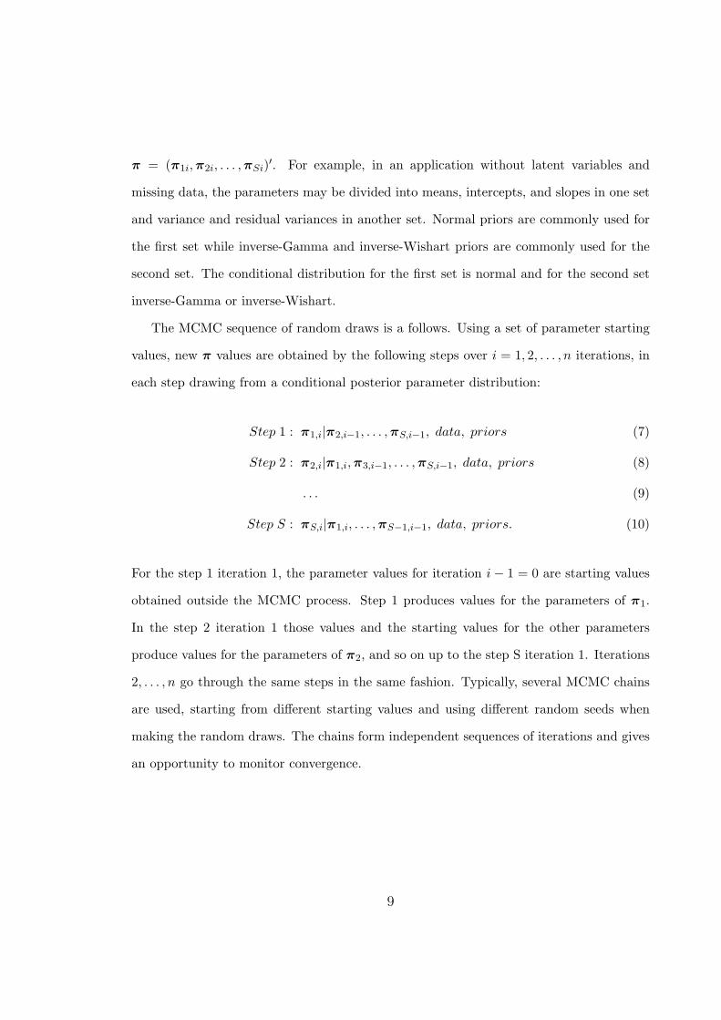
The MCMC sequence of random draws is a follows. Using a set of parameter starting

values, new π values are obtained by the following steps over i = 1, 2, . . . , n iterations, in

each step drawing from a conditional posterior parameter distribution:

Step 1 : π1,i|π2,i−1, . . . ,πS,i−1, data, priors (7)

Step 2 : π2,i|π1,i,π3,i−1, . . . ,πS,i−1, data, priors (8)

. . . (9)

Step S : πS,i|π1,i, . . . ,πS−1,i−1, data, priors. (10)

For the step 1 iteration 1, the parameter values for iteration i− 1 = 0 are starting values

obtained outside the MCMC process. Step 1 produces values for the parameters of π1.

In the step 2 iteration 1 those values and the starting values for the other parameters

produce values for the parameters of π2, and so on up to the step S iteration 1. Iterations

2, . . . , n go through the same steps in the same fashion. Typically, several MCMC chains

are used, starting from different starting values and using different random seeds when

making the random draws. The chains form independent sequences of iterations and gives

an opportunity to monitor convergence.

9

2.1.3 Assessing convergence

In the analyses of this paper convergence is investigated in the following way. Consider

n iterations in m chains, where πij is the value of parameter π in iteration i of chain j.

Define the within- and between-chain variation as

π.j =1n

n∑i=1

πij , (11)

π.. =1m

m∑j=1

π.j , (12)

W =1m

m∑j=1

1n

n∑i=1

(πij − π.j)2, (13)

B =1

m− 1

m∑j=1

(π.j − π..)2. (14)

Convergence is determined using the Gelman-Rubin convergence diagnostic (Gelman &

Rubin (1992); Gelman et al., 2004). This considers the potential scale reduction factor

(PSR),

PSR =

√W +B

W, (15)

where a PSR value not much larger than 1 is considered evidence of convergence. Gelman

et al. (2004) suggests 1.1, or smaller values for all parameters. This means that convergence

is achieved when the between-chain variation is small relative to the within-chain variation.

Gelman et al. (2004) use a slightly different definition of their potential scale reduction R,

but the difference relative to (15) is a negligible factor of n/(n − 1). It may be the case,

however, that PSR convergence observed after n iterations may be negated when using

more iterations. Because of this, a longer chain should be run to check that PSR values

are close to 1 in a long sequence of iterations.

10

2.1.4 Model fit

Model fit assessment is possible using Posterior Predictive Checking (PPC) introduced

in Gelman, Meng and Stern (1996). With continuous outcomes, PPC as implemented in

Mplus builds on the standard likelihood-ratio χ2 statistic in mean- and covariance-structure

modeling. This PPC procedure is described in Scheines et al. (1999) and Asparouhov and

Muthen (2010a, b) and is briefly reviewed here. Gelman et al. (2004) presents a more

general discussion of PPC, not tied to likelihood-ratio χ2.

A Posterior Predictive p-value (PPP) of model fit can be obtained via a fit statistic

f based on the usual likelihood-ratio χ2 test of an H0 model against an unrestricted H1

model. Low PPP indicates poor fit. Let f(Y, X, πi) be computed for the data Y, X

using the parameter values at MCMC iteration i. At iteration i, generate a new data set

Y ∗i of synthetic or replicated data of the same sample size as the original data. In this

generation the parameter values at iteration i are used. For these replicated data the fit

statistic f(Y ∗i , X, πi) is computed. This data generation and fit statistic computation

is repeated over the n iterations, after which PPP is approximated by the proportion of

iterations where

f(Y, X, πi) < f(Y ∗i , X, πi). (16)

In the Mplus implementation (Asparouhov & Muthen, 2010a) PPP is computed using

every 10th iteration among the iterations used to describe the posterior distribution of

parameters. A 95% confidence interval is produced for the difference in the f statistic for

the real and replicated data. A positive lower limit is in line with a low PPP and indicates

poor fit. An excellent-fitting model is expected to have a PPP value around 0.5 and an f

statistic difference of zero falling close to the middle of the confidence interval.

It should be noted that the PPP value does not behave like a p-value for a χ2 test of

11

model fit (see also Hjort et al., 2006). The type I error is not 5% for a correct model.

There is not a theory for how low PPP can be before the model is significantly ill-fitting

at a certain level. In this sense, PPP is more akin to a structural equation modeling

fit index rather than a χ2 test. Empirical experience with different models and data

has to be established for PPP and some simulation studies are presented here. From

these simulations and further ones in Asparouhov and Muthen (2010b), however, the usual

approach of using p-values of 0.05 or 0.01 appears reasonable.

3 BSEM: A more flexible SEM approach

A new approach to structural equation modeling based on Bayesian analysis is described

below. It is intended to produce an analysis that better reflects the researcher’s theories

and prior beliefs. It does so by systematically using informative priors for parameters that

should not be freely estimated according to the the researcher’s theories and prior beliefs.

In a frequentist analysis such parameters are typically fixed at zero or are constrained to

be equal to other parameters. If these parameters were all freed the model would in fact

not be identified. The Bayesian analysis, however, identifies the model by substantively-

driven small-variance priors. The proposed approach is referred to as BSEM for Bayesian

structural equation modeling. It should be recognized, however, that BSEM refers to the

specific Bayesian approach proposed here of using informative, small-variance priors to

reflect the researcher’s theories and prior beliefs.

BSEM is applicable to any constrained parameter in an SEM. This paper focuses on

parameters in the measurement part, but restrictions in the structural part can also be

considered. Three types of model features are considered: Cross-loadings in CFA, residual

correlations in CFA, and measurement non-invariance.

12

3.1 Informative priors for cross-loadings in CFA

An analyst who is used to frequentist methods such as ML may at first feel uncomfortable

specifying informative priors. It is argued here, however, that a user of CFA is in a sense

already engaged in specifying such priors. Consider the confirmatory factor analysis model

for an observed p-dimensional vector yi of factor indicators for individual i,

yi = ν + Λ ηi + εi,

E(yi) = ν + Λ α,

V (yi) = Λ Ψ Λ′ + Θ, (17)

where ν is an intercept vector, Λ a loading matrix, ηi is an m-dimensional factor vector,

εi is a residual vector, α is a factor mean vector, Ψ is a factor covariance matrix, and

Θ is a residual covariance matrix. Here, ε and η are assumed normally distributed and

uncorrelated.

Drawing on substantive theory, zero cross-loadings in Λ are specified for the factor

indicators that are hypothesized to not be influenced by certain factors. An exact zero

loading can be viewed as a prior distribution that has mean zero and variance zero. A

prior that probably more accurately reflects substantive theory uses a mean of zero and

a normal distribution with small variance. Figure 2 shows an example where a loading

λ ∼ N(0, 0.01) so that 95% of the loading variation is between −0.2 and +0.2. Using

standardized variables, a loading of 0.2 is considered a small loading, implying that this

prior essentially says that the cross-loading is close zero, but not exactly zero. The prior

is strongly informative, but it is not assumed that the parameter is zero.

[Figure 2 about here.]

It is well-known that in frequentist analysis freeing all cross-loadings in a CFA model

such as Table 2 leads to a non-identified model because the m2 restrictions, where m is the

13

number of factors, necessary to eliminate indeterminacies are not present (see, e.g., Hayashi

& Marcoulides, 2006). Using small-variance priors for all cross-loadings, however, brings

information into the analysis which avoids the non-identification problem. The choice of

variance for the prior should correspond to the the researcher’s theories and prior beliefs.

As stated above, the variance of 0.01 produces a prior where 95% lies between −0.2 and

+0.2. Other choices are shown in Table 1.

[Table 1 about here.]

A smaller variance may not let cross-loadings escape sufficiently from their zero

prior mean, producing a worse Posterior Predictive p-value. A larger variance may

let a cross-loading have too large of a probability of having a substantial value. For

example, a variance of 0.05 corresponds to 95% lying between −0.44 and +0.44, which

on a standardized variable scale approaches a major loading size. When the variance is

increased, the prior contributes less information so that the model gets closer to being

non-identified which causes non-convergence of the MCMC algorithm. It should be noted

that the prior variance should be determined in relation to the scale of the observed and

latent variables. A prior variance of 0.01 corresponds to small loadings for variables with

unit variance, but it corresponds to a smaller loading for an observed variable with variance

larger than one. This means that for convenience observed variables may be brought to

a common scale either by multiplying them by constants, or standardizing if the model is

scale free.

BSEM has an additional advantage. It produces posterior distributions for cross-

loadings which can be used in line with modification indices to free parameters for which

the credibility interval does not cover zero. Modification indices pertain to freeing only one

parameter at a time and a long sequence of model modification is often needed, running

the risk of capitalizing on chance (see, e.g., McCallum, 1992). In contrast, the small-

variance prior approach provides information on model modification that considers the

14

fixed parameters jointly in a single analysis.

3.2 Informative priors for residual covariances in CFA

An analogous idea can also be used to study residual correlations among factor indicators.

In (17), the residual covariance matrix Θ is commonly assumed to be diagonal. Some

residuals may, however, be correlated due to the omission of several minor factors. It is

difficult to foresee which residuals should be covaried and freeing all of them leads to a

non-identified model in the conventional ML framework. BSEM resolves this.

Instead of assuming a diagonal residual covariance matrix, a more realistic covariance

structure model may be expressed as

V (yi) = Λ Ψ Λ′ + Ω + Θ∗, (18)

where Ω is a covariance matrix for the minor factors, not assumed to be diagonal, and

Θ∗ is a diagonal covariance matrix. Here, a freely estimated Ω is not separately identified

from Λ, Ψ, and Θ∗. In Bayesian analysis, however, Ω can be given an informative prior

using the inverse-Wishart distribution so that the posterior distribution can be obtained.

In this way, the diagonal and off-diagonal elements of Ω are restricted to small values.

This implies that the residual covariance matrix Ω+Θ∗ contains residual covariances that

are allowed to deviate to a small extent from zero means. Sufficiently stringent priors

for the off-diagonal elements are needed so that the essential correlations are channeled

via Λ Ψ Λ′. The sums on the diagonal of Ω + Θ∗ produce the residual variances. The

inverse-Wishart distribution is described in the Appendix.

The BSEM approach for residual covariances outlined in connection with (18) will be

referred to as Method 1. A more direct method, Method 2, applies an inverse-Wishart

prior directly on Θ in (17). This approach has been discussed in Press (2003; chapter

15

15). A disadvantage of both Method 1 and Method 2 is that particular residual covariance

elements cannot be given their own priors. For example, an analysis may show that some

residual covariances should be freely estimated with non-informative priors because they

have 95% credibility intervals that do not cover zero. To this aim, Method 3 makes it

possible to specify element-specific normal priors for the residual covariances. Mplus allows

two different algorithms for Method 3, a random-walk algorithm (Chib & Greenberg, 1988)

and a proposal prior algorithm (Asparouhov & Muthen, 2010a).

The choice of inverse-Wishart prior should be made to reflect prior beliefs in the

potential magnitude of residual covariances. This is accomplished by using a sufficiently

large choice for the degrees of freedom (df) of the inverse-Wishart distribution. To obtain

a proper posterior where the marginal mean and variance is defined, df ≥ p+4 needs to be

chosen, where p is the number of variables y. The prior means for the residual covariances

can be chosen as zero and the degree of informativeness specified using the df which affects

the marginal prior variance via df−p. For example, (28) of the Appendix shows that using

the inverse-Wishart prior IW (I, df) with df = p + 6 gives a prior standard deviation of

0.1, so that two standard deviations below and above the zero mean correspond to the

residual covariance range of −0.2 to +0.2. The effect of priors is relative to the variances

of the ys. For scale-free models, the variables may be standardized before analysis. For

larger sample sizes, the prior needs to use a larger df to give the same effect.

Method 1 and 2 both use conjugate priors and generally produce good mixing in the

MCMC chain. One advantage of Method 1 over Method 2 is that the prior for the total

residual variance is not tied to the prior of the residual covariances because of the fact that

the residual covariance has two components that have different priors. Method 2, however,

is simpler. Both versions of Method 3, random walk and proposal prior algorithm, are based

on the Metropolis-Hastings algorithm and that generally yields somewhat worse mixing

performance. The random walk algorithm has difficulty converging or converges very slowly

16

when the variance-covariance matrix has a large number of parameters. However when a

large number of parameters have small prior variance the convergence is fast. The proposal

prior algorithm generally mixes fast, but it does not work well when the prior variance is

very small.

When estimating the above models all the algorithms are applied to extreme conditions

with a nearly unidentified model and near zero prior variance. Convergence of the MCMC

sequence should be carefully evaluated and automated convergence criteria such as PSR

should not be trusted. The models should be estimated with a large number of MCMC

iterations, for example, 50000.

3.3 Informative priors for direct effects in MIMIC modeling

BSEM can be extended to include equality constraints. A typical SEM example is multiple-

group analysis with measurement invariance. It is common to find small deviations from

exact invariance that cause rejection by the ML LRT. Consider the multiple-group model

extension of (17) for individual i in group g (g = 1, 2, . . . , G),

yig = νg + Λg ηig + εig,

E(yig) = νg + Λg αg,

V (yig) = Λg Ψg Λ′g + Θg. (19)

Bayesian analysis can be used to relax the hypothesis of exact measurement invariance,

modifying the model as

yig = ν + νg + (Λ + Λg) ηig + εig, (20)

17

where for g = 2, 3, . . . G, νg and Λg are measurement intercept vectors and loading

matrices, respectively, that have small-variance priors, representing minor deviations from

the intercept vectors and loading matrices of the reference group g = 1.

In this paper the special case of intercept non-invariance is studied, assuming invariance

of factor loadings and residual covariance matrices. In this case the modeling can be

handled by letting the grouping variables be covariates that influence the factors, also

referred to as MIMIC modeling (see, e.g., Muthen, 1989). Here, non-invariance is defined

as direct effects from covariates to the factor indicators. Unlike with ML, all direct effects

can be included and given small-variance priors such as ∼ N(0, 0.01).

4 Study 1: Cross-loadings in CFA

4.1 Holzinger-Swineford mental abilities example: ML anal-

ysis

The first example uses data from the classic 1939 factor analysis study by Holzinger and

Swineford (1939). Twenty-six tests intended to measure a general factor and five specific

factors were administered to seventh and eighth grade students in two schools, the Grant-

White school (n = 145) and the Pasteur school (n = 156). Students from the Grant-White

school came from homes where the parents were mostly American-born, whereas students

from the Pasteur school came largely from working-class parents of whom many were

foreign-born and where their native language was used at home.

Factor analyses of these data have been described e.g. by Harman (1976; pp. 123-132)

and Gustafsson (2002). Of the 26 tests, nineteen were intended to measure four domains,

five measured general deduction, and two were revisions/new test versions. Typically, the

last two are not analyzed. Excluding the five general deduction tests, 19 tests measuring

four domains are considered here, where the four domains are spatial ability, verbal ability,

18

speed, and memory. The design of the measurement of the four domains by the 19 tests is

shown in the factor loading pattern matrix of Table 2. Here, an X denotes a free loading

to be estimated and 0 a fixed, zero loading. This corresponds to a simple structure CFA

model with variable complexity one, that is, each variable loads on only one factor.


Using maximum-likelihood estimation, the model fit using both confirmatory factor

analysis (CFA) and exploratory factor analysis (EFA) is reported in Table 3 for both

the Grant-White and Pasteur schools. It is seen that the CFA model is rejected by the

likelihood-ratio χ2 test in both samples. Given the rather small sample sizes, one cannot

attribute the poor fit to the χ2 test being overly sensitive to small misspecifications due

to a large sample size as is often done. The common fit indices RMSEA and CFI are also

not at acceptable levels. In contrast to the CFA, Table 3 shows that the EFA model fits

the data well in both schools.


Table 4 shows the EFA factor solution for both schools using the Geomin rotation.

The Quartimin rotation gives similar results. For a description of these rotations, see,

e.g., Asparouhov and Muthen (2009). The table shows that the major loadings of the

EFA correspond to the hypothesized four-factor loading pattern (bolded entries). Several

of the tests, however, also have cross-loadings on other factors. There are six significant

cross-loadings for the Grant-White solution and ten for the Pasteur solution. This explains

the poor fit of the CFA model.

The question arises how to go beyond postulating only the number of factors as in EFA

and maintain the essence of the hypothesized factor loading pattern without resorting

to an exploratory rotation. Cross-loadings need to be allowed, but a model with freely

19

estimated cross-loadings is not identified. The proposed Bayesian solution to this problem

is presented next.


4.2 Holzinger-Swineford mental abilities example: Bayesian

analysis

This section uses data from the Grant-White and Pasteur schools of the Holzinger-

Swineford study to illustrate the Section 3.1 BSEM approach with informative cross-

loading priors. The factor loading pattern of the four-factor model of Table 2 is used.

Table 5 repeats the fit statistics for the ML CFA and EFA and adds the fit statistics for

Bayesian analysis using both the original CFA model and the proposed CFA model with

informative, small-variance priors for cross-loadings. The cross-loading priors use variances

0.01. Standardized variables are analyzed.

Table 5 shows that the Bayesian analysis of the CFA model with exact zero cross-

loadings gives almost zero Posterior Predictive p-values in line with the ML CFA. In

contrast, for the proposed Bayesian CFA with cross-loadings model fit is acceptable in

that the Posterior Predictive p-value is 0.343 for Grant-White and 0.068 for Pasteur.

The Bayesian estimates can be used as fixed parameters in an ML analysis in order

to get the likelihood-ratio test (LRT) value for the Bayes solution. They can be viewed

as a measure of fit that can be compared to the ML likelihood-ratio χ2 values. It is seen

in Table 5 that the Bayesian LRT values for the CFA model are close to those of ML χ2

values. In contrast, the Bayesian LRT values for the model with cross-loadings shows a

great improvement, falling halfway between the ML CFA and EFA χ2 values.


20

The Bayes factor solutions for the two schools are shown in Table 6. It is interesting to

compare the Bayes solution to the ML EFA solution of Table 4. The Bayes factor loadings

are on the whole somewhat larger than those for ML and there are far fewer significant

cross-loadings. For ML, there are six significant cross-loadings for Grant-White and ten

for Pasteur, whereof only three appear for both solutions. Because they appear for both

schools, a researcher may be tempted to free these three cross-loadings. For Bayes, the

Grant-White sample has only two cross-loadings that are significant (have a 95% credibility

interval that does not cover zero) and Pasteur has none. Because of the lack of agreement,

freeing the two could be capitalizing on chance and is not necessary on behalf of model fit.

Bayes clearly gives a simpler pattern than ML EFA for these data.

It should be emphasized that cross-loadings that are found to be important in

BSEM (the 95% credibility interval does not cover zero and the cross-loading has strong

substantive backing) can be freely estimated while keeping small-variance priors for other

cross-loadings. This should improve the results because the small-variance prior results

in a too small estimate for such a cross-loading. Monte Carlo simulations show that this

gives better estimation.

The ML EFA factor correlations are smaller than the Bayesian factor correlations. The

greater extent of cross-loadings in the EFA may contribute to the lower factor correlations

in that less correlation among variables need to go through the factors. The Bayesian

factor correlations are not excessively high because the factors are expected to correlate

to a substantial degree according to theory. Holzinger and Swineford (1939) hypothesized

that the variables are all influenced by a deductive factor that in the current model is not

partialled out of the four factors.

The choice of cross-loading prior variance should be linked to the researcher’s prior

beliefs. It could be argued, however, that the choice of a variance of 0.01 resulting in 95%

limits of ±0.20 is not substantially different from a variance of 0.02 resulting in 95% limits

21

of ±0.28; see Table 1. It may therefore be of interest to vary the prior variance to study

sensitivity in the results. Increasing the prior variance tends to increase the variability of

the estimates and affect the Posterior Predictive p-value. At a certain point of increasing

the prior variance, the model is not sufficiently identified and the MCMC algorithm tends

to give non-convergence. In the Grant-White data the prior variance of 0.01 (95% limit

±0.20) used for the Table 6 results gives a p-value of 0.343 with factor correlations in the

range 0.4 − 0.6. A prior variance of 0.02 (95% limit ±0.28) gives a p-value of 0.431 with

factor correlations around 0.6. For the Pasteur data convergence is not obtained when

increasing the prior variance above 0.01. Analyzing the two schools together, yielding a

larger sample of n = 301, the size of the factor correlations do not change much when

varying the prior variance from 0.01 to 0.07. This is in line with findings from Monte

Carlo simulations (not shown) where the prior variance is varied for the model used in

Section 4.3 with cross-loadings 0.3.

In summary, BSEM provides a simpler model and a model that better fits the

researcher’s prior beliefs than ML. BSEM provides an approach which is a compromise

between that of EFA and CFA. The ML CFA rejects the hypothesized model, presumably

because it is too strict. ML EFA does not reject the model, but the model does not match

the researcher’s prior beliefs because it only postulates the number of factors, not where the

large and small loadings should appear. Furthermore, ML EFA provides a solution through

a mechanical rotation algorithm, whereas BSEM uses priors to represent the researcher’s

beliefs.


4.3 Cross-loading simulations

This section discusses Monte Carlo simulations of BSEM applied to factor modeling with

cross-loadings. The aim is to demonstrate that the proposed approach provides good

22

results for data with known characteristics.

The factor loading pattern of Table 7 is considered where X denotes a major loading and

x cross-loadings. The major loadings are all 0.8. The size of the three cross-loadings are

varied as 0.0, 0.1, 0.2, and 0.3 in different simulations. The observed and latent variables

have unit variances so the loadings are on a standardized scale. A cross-loading of 0.1

is considered to be of little importance, a cross-loading of 0.2 of some importance, and a

cross-loading of 0.3 of importance (Cudeck & O’Dell, 1994). The correlations among the

three factors are all 0.5. The factor metric is determined by fixing the first loading for each

factor at 0.8. Non-informative priors are used for all parameters except for cross-loadings

when those are included in the analysis. Sample sizes of n = 100, n = 200 and n = 500

are studied.

A total of 500 replications are used. The reported parameter estimate is the median in

the posterior distribution for each parameter. The key result is what frequentists would

refer to as the 95% coverage, that is, the proportion of the replications for which the 95%

Bayesian credibility interval covers the true parameter value used to generate the data.

For cross-loadings it is also of interest to study what corresponds to power in a frequentist

setting. This is computed as the proportion of the replications for which the 95% Bayesian

credibility interval does not cover zero. Results are reported only for a representative set

of parameters or functions of parameters: the major loading of y2, the cross-loading for y6,

the variance for the first factor, and the correlation between the first and second factor.


4.3.1 Bayes, non-informative priors

As a first step, consider Bayesian analysis without informative priors and ignoring cross-

loadings. The top part of Table 8 shows the summaries of the simulations for n = 100,

n = 200, and n = 500 when data have been generated with zero cross-loadings. Here,

23

the analysis is correctly specified and close to 95% coverage is obtained for all free

parameters. The cross-loadings are not estimated in this case so that this entry should be

ignored. Posterior Predictive p-values for the model fit assessment are 0.036, 0.032, and

0.024, respectively for the three sample sizes, that is, reasonably close to the nominal 5%

level. Table 8 shows that Bayesian analysis with non-informative priors works well in this

example.

With cross-loadings of 0.1 the bottom part of Table 8 shows the effects of model

misspecification in that the coverage is less good. Again, the cross-loadings are not

estimated in this case so that this entry should be ignored. Posterior Predictive p-values

for the model fit assessment are 0.056, 0.080, and 0.262, respectively for the three sample

sizes. This shows limited power to reject the incorrect model. On the other hand, the

misspecification is deemed of little importance given the small size of the cross-loadings.

With cross-loadings of 0.2 (not shown) the Posterior Predictive p-value is 0.196 for

n = 100, 0.474 for n = 200, and 0.984 for n = 500, showing excellent power at higher sample

sizes. With cross-loadings of 0.3 the Posterior Predictive p-value is 0.544 for n = 100, 0.944

for n = 200, and 1.000 for n = 500, showing that the power is excellent when the cross-

loading is of an important magnitude.


4.3.2 Comparing ML to Bayes

Model fit assessment comparing ML to Bayesian analysis with non-informative priors is

shown in Table 17. The correctly specified model with zero cross-loadings shows an inflated

ML p-value of 0.172 at n = 100. This small-sample bias is well-known for ML χ2 testing

(see, e.g., Scheines et al., 1999). The Posterior Predictive p-value of 0.036 based on the

Bayesian analysis does not show the same problem. For the 0.1 size of the cross-loadings,

which is deemed of little substantive importance, ML rejects the model 46% of the time

24

at n = 500. This reflects the common notion that the ML LRT χ2 can be oversensitive

to small degrees of model misspecification. For the important degree of misspecification

with cross-loading 0.3, the ML test is more powerful than Bayes, but the Bayes power is

sufficient for sample sizes of at least n = 200.


Table 10 shows ML model estimation results as a comparison to the Bayesian analysis

with non-informative priors presented earlier. For both the correctly specified model with

zero cross-loadings and for the misspecified model with cross-loadings 0.1 the ML coverage

is close to that of Bayes. The mean-square-error (MSE) is also similar for Bayes and ML.

Based on this, there is no reason to prefer one method over the other.


4.3.3 Bayes, informative priors

As the next step, the proposed BSEM approach of using Bayesian analysis with informative,

small-variance priors for the cross-loadings is applied. Table 11 shows that as compared to

Table 8, the coverage remains largely the same for the top part of the table corresponding to

the correctly specified analysis with zero cross-loadings. For cross-loadings of 0.1, however,

the bottom part of the table shows that coverage has improved by the introduction of

informative, small-variance priors for the cross-loadings. The coverage is acceptable also

for the cross-loading. The power to detect the cross-loading is, however, small at this low

cross-loading magnitude, 0.038, 0.098 and 0.176, respectively for the three sample sizes.

The Posterior Predictive p-value is on the low side in all four cases.

It is interesting to compare the coverage results for the four parameters in the case of

cross-loadings 0.1 given in the Table 11 for BSEM and in Table 10 for the ML approach.

It is seen that ML is outperformed by BSEM by its use of informative priors.

25


Table 12 shows the results of BSEM where data have been generated with larger cross-

loadings of 0.2 and 0.3. Here the coverage is also good with the exception of the cross-

loadings. For the cross-loadings, however, the focus is on power as shown in the last

columns. For a cross-loading of 0.2 a sample size of n = 500 is needed to obtain power

above 0.8. For a cross-loading of 0.3 a sample size of n = 200 is sufficient to obtain power

above 0.8. This shows that the approach of using informative, small-variance priors for

cross-loadings leads to a successful way to modify the model, allowing free estimation of

the indicated cross-loadings.

The point estimates indicate that the key parameter of factor correlation is overesti-

mated. Note, however, that given the power to detect cross-loadings, estimating them

freely results in good point estimates for factor correlations.

In summary, the cross-loading simulation study shows that the Bayesian analysis

performs well. It also shows that in terms of parameter coverage and for the case of

small cross-loadings ML is inferior to BSEM. In terms of model testing, BSEM avoids the

small-sample inflation of the ML χ2 and also avoids the ML χ2 sensitivity to rejecting a

model with an ignorable degree of misspecification.


5 Study 2: Residual correlations in CFA

5.1 British Household Panel Study (BHPS) big-five person-

ality example: ML analysis

A second example uses data from the British Household Panel Study (BHPS) of 2005

and 2006. A 15-item, five-factor instrument uses three items to measure each of the ”big-

26

five” personality factors: agreeableness, conscientiousness, extraversion, neuroticism, and

openness. Each item uses the question ”I see myself as someone who . . .” followed

by a statement. There are seven response categories ranging from 1 ”does not apply” to

7 applies perfectly”. A total of 14, 021 subjects are included. The big-five factors are

expected a priori to have low correlations and are known to be related to gender and age;

see, e.g. Marsh, Nagengast, and Morin (2010). For simplicity, the current analyses hold

age constant by considering the subgroup of ages 50-55. This produces a sample of n = 691

females and n = 589 males.

The item wording and hypothesized loading pattern are shown in Table 13. For all

factors except openness, there are two positively-worded items and one negatively-worded

item. Marsh, Nagengast, and Morin (2010) suggest that the four negatively-worded items

may a priori have correlated residuals (correlated uniquenesses) when applying factor

analysis.


Using maximum-likelihood estimation, model fit using confirmatory factor analysis

(CFA), CFA with correlated uniquenesses (CU) among the negatively-worded items, and

exploratory factor analysis (EFA) is reported in Table 14. It is seen that the fit is not

acceptable for either of the two CFA models as judged by χ2 or the two model fit indices.

The EFA model is also rejected by χ2 and only marginally acceptable for males when

judged by RMSEA or CFI.


An interesting finding is that the EFA solutions for females and males do not fully

capture the hypothesized factors. This is the case using the Geomin rotation as well as

using Quartimin and Varimax. The Geomin rotation for each gender is shown in Table 15.

The bolded entries are loadings that are the largest for the item. Comparing to Table 13

27

it is seen that only the factors extraversion, neuroticism, and openness are found, not the

agreeableness and conscientiousness factors. A possible reason for this is the existence

of correlated residuals among the items. As the CFA with CUs model showed, however,

allowing residual correlations among the reverse-coded items is not sufficient. It is likely

that in addition to the big-five factors the personality instrument measures many minor

factors.

The question arises how correlated residuals can be accounted for while maintaining the

hypothesized factor loading pattern. A model with all residual correlations freely estimated

is not identified. The proposed BSEM solution to this problem is presented next.


5.2 British Household Panel Study (BHPS) big-five person-

ality example: Bayesian analysis

This section uses the big-five personality data in the British Household Panel Study (BHPS)

to illustrate the BSEM approach of Section 3.2 with an informative prior for the residual

covariance matrix. Method 2 is used with an inverse-Wishart prior IW (I, df) with df =

p+ 6 = 21, corresponding to prior means and standard deviations for residual covariances

of zero and 0.1, respectively (see Appendix, (28)). Standardized variables are analyzed.

Because of high auto-correlation among the MCMC iterations, only every 10th iterations is

used with a total of 100,000 iterations to describe the posterior distribution. Informative

cross-loading priors are also used with prior distributions N(0, 0.01).

The Posterior Predictive p-values are 0.534 and 0.518, respectively for females and

males indicating a good match between the model and the data. For the two samples 17

and 37 residual covariances, respectively, were found significant in the sense of the 95%

Bayesian credibility interval not covering zero. The average absolute residual correlation

28

(range) is 0.329 (−0.462 to 0.647) for females and 0.285 (−0.484 to 0.590) for males. For

both genders only one residual correlation exceeds 0.5 in absolute value. This suggests that

many small residual correlations need to be included in the factor model, as was expected.

The fact that these residual correlations are left out in the ML analyses may contribute to

the poor ML fit and the poor ML EFA loading pattern recovery.

Table 16 gives the results for the female and male samples. Standardized loadings

are presented so that the results can be compared to the ML EFA of Table 15. The

hypothesized major loadings are all recovered at substantial values with no significant

cross-loadings. The factor correlations are all small to moderate as was expected. The

extraversion, neuroticism, and openness factors that were recovered in the ML EFA of

Table 15 have lower correlations in the Bayesian solution than in the ML EFA.

In summary, BSEM provides a solution that better fits the researcher’s prior beliefs

than ML. The ML CFA rejects the hypothesized model, presumably because it is too

strict in terms of requiring exactly zero residual covariances. ML EFA does not recover

the researcher’s hypothesized big-five factor pattern.


5.3 Residual correlations simulations

This section discusses Monte Carlo simulations of the BSEM approach to factor modeling

with residual correlations. A factor model with 10 variables and two factors is used,

where the first five variables load on only the first factor and the second five variable load

only on the second factor. The loadings are all 0.8, the factor variances are 1, and the

factor correlation is 0.5. The residual variances are 0.36 so that observed variables all have

variances 1. Two residual covariances (correlations) are included, one for the first and sixth

variables and one for the second and seventh variables. In this way, ignoring the residual

covariances in the modeling tends to inflate the factor correlation. An example would be

29

an instrument administered at two time points, where some variables have residuals that

are correlated over time. Residual correlations of 0.0, 0.1, and 0.3 are considered together

with sample sizes n = 200 and n = 500. A total of 500 replications are used and the

results presented in the format used for the cross-loading simulations. The simulations

present results for all three methods discussed in Section 3.2. For Method 1, both a more

informative prior with df = 30 and a less informative prior with df = 14 (= p + 4) is

studied. For Method 2, df = 30 is used. For Method 3, the normal prior variance is set at

0.001.

5.3.1 Comparing ML to Bayes

As a first step, model testing using ML and Bayes with non-informative priors is compared

for both correctly and misspecified models. Table 17 shows that for residual correlations of

0.0, both ML and Bayes give acceptable rejection rates with the correctly specified model.

Both ML and Bayes reject the model with ignorable residual correlations of 0.1, although

ML is more sensitive to this misspecification. For the larger misspecification with residual

correlations of 0.3, both ML and Bayes show sufficient power to reject the model at both

n = 200 and n = 500.


Table 18 and Table 19 summarize the simulation results for BSEM using Method 1

with residual correlations 0.1 and 0.3, respectively. The top two panels give results for

df = 30 and the bottom two panels for df = 14.

Table 18 shows good coverage for all parameters except the residual covariance. There

is sufficient power to detect the residual covariance of 0.1 at n = 500. There is no important

difference between using df = 30 and df = 14, except that the point estimate and the power

for the residual covariance is slightly better for the less informative prior with df = 14.

30

Table 19 shows acceptable coverage when using the less informative prior with df =

14, except for the residual correlation. The power to detect the residual correlations is,

however, excellent in all cases. For the more informative prior with df = 30, the coverage is

less good. The key parameter of the factor correlation shows an important overestimation,

which is also seen with df = 14.



Table 20 shows the simulation results for BSEM Methods 2 and 3 using residual

correlations of 0.3. The 5% reject proportion for the Posterior Predictive p-value is 0 in

all cases. For Method 2 the results are very good except for the residual covariance being

underestimated and having poor coverage. The power to detect it is, however, excellent.

The factor correlation is also somewhat underestimated. Method 2 performs considerable

better than Method 1 as seen in Table 19. The Method 3 results are somewhat worse than

those of Method 1 for df = 14, with poorer performance for the residual covariance and

the factor correlation. The power to detect the residual covariance is, however, excellent

also for Method 3. It should be noted that Method 3 is the only one of the three methods

that can let such a residual covariance be freely estimated, that is, using a non-informative

prior. Using a less informative Method 3 prior with a larger variance of 0.01 did not alter

the results very much. In summary, Method 2 performs the bests of the three methods

and Method 3 the worst for this simulation setting.


Table 21 demonstrates that Method 3 works well when the two residual covariances are

freely estimated, that is, using non-informative priors. The remaining residual covariances

are using the same informative priors as before. Results are shown for n = 200 and n = 500.


31

6 Study 3: Direct effects in MIMIC modeling

6.1 Antisocial behavior example: ML analysis

As a third example consider Antisocial Behavior (ASB) data taken from the National

Longitudinal Survey of Youth (NLSY), sponsored by the Bureau of Labor Statistics. NLSY

data for the analysis include 17 antisocial behavior items that were collected in 1980 when

respondents were between the ages of 16 and 23. The ASB items assess the frequency of

various behaviors during the past year. In these analyses, the ASB items are dichotomized

0/1 with 0 representing never in the last year. The sample analyzed here consists of

7,326 respondents with complete data on the antisocial behavior items and the background

variables of age, gender, and ethnicity. The dichotomous responses are modeled using a

probit link as in Muthen (1989), applying maximum-likelihood estimation as in IRT.

EFA of the 17 dichotomous ASB items suggests three factors: property offense, person

offense, and drug offense. Table 22 shows the item wording and the EFA solution using

maximum-likelihood estimation and the Geomin rotation.


Because of the heterogeneity of the national sample, it is of interest to study to which

extent the ASB items exhibit measurement invariance with respect to the subject groupings

provided by the age, gender, and ethnicity variables. Non-invariance is also referred to as

differential item functioning (DIF). DIF can be studied using a three-factor CFA model

where the factors are regressed on the covariates of age, gender, and ethnicity. DIF is

present when a covariate has a direct effect on an item, over and above the indirect effect

via the factors (see, e.g., Muthen, 1989).

A search for the need to include direct effects to represent DIF can involve examining

modification indices and/or exploring the significance of direct effects by regressing one

item at a time on all covariates. Using a relatively untested measurement instrument in

32

a national sample, however, is likely to produce many instances of direct effects (DIF),

leading to a long search that may be capitalizing on chance. On the other hand, allowing

all direct effects to be freely estimated gives a non-identified model. The proposed Bayesian

solution to this problem is presented next.

6.2 Antisocial behavior example: Bayesian analysis

BSEM is applied here to direct effects in the antisocial behavior example. The 17 binary

items measure the three factors of property offense, person offense, and drug offense which

are related to the covariates age, gender and ethnicity. All direct effects from the covariates

to the items are included using normal priors with mean zero and variance 0.04 in line with

the discussion in Section 6.3. In addition, cross-loadings are included with normal priors

of mean zero and variance 0.01. The major loadings are chosen as follows for each factor,

based on EFA. The Property factor is measured by property, shoplift-gt50, con-goods.

The Person factor is measured by fight, force-injure. The Drugs factor is measured by

pot-solddrug.

Table 23 shows the factor loadings and factor correlations. The top part of Table 24

shows the effects of the covariates on the factors, whereas the bottom part shows the

direct effects of the covariates on the factor indicators. The direct effects for which the 95%

Bayesian credibility interval does not cover zero are bolded, showing a total of twelve effects.

This illustrates the importance of allowing for all possible direct effects using informative,

small-variance priors. Modifying the model without any direct effects using modification

indices and freeing one parameter at a time leads to a long model modification process.

Further research is of interest to see if such an approach is more prone to capitalizing on

chance than the BSEM approach.



33

6.3 Direct effect simulations

This section discusses Monte Carlo simulations of the BSEM approach to a MIMIC model

with direct effects. The same factor loading pattern as in Table 7 is considered, except with

no cross-loadings. The correlations among the three factors are all 0.5 and their variances

are one. The factor metric is determined by fixing the first loading for each factor at 1.0.

The factor model uses a probit specification. The loadings are all 1.0, which is close to the

real antisocial behavior data. There is a single binary covariate and there are three direct

effects to y1, y6, and y11. The direct effects are 0.4 which corresponds to a small effect size

in terms of Cohen’s d considering the mean difference in the binary factor indicators. The

value 0.4 is chosen as follows. The variance for an underlying conditionally normal latent

response variable y∗ in the probit factor model is the variance explained by the factor(s)

plus a residual variance fixed at unity. For the loadings chosen the variance explained by

the factors is 1 and therefore the total variance is 2. With a small effect size defined as

approximately 0.3 of a y∗ standard deviation, a value of 0.42 is obtained, which is rounded

off to 0.4.

Non-informative priors are used for all parameters except for direct effects. The

informative prior for each direct effect is taken to be normal with mean zero and variance

0.04 determined as follows. The direct effect of 0.4 is taken to be in the tail of the prior in

line with how the cross-loading of 0.2 was in the tail of its prior. Letting the 95% limit be

±0.4 results in a prior variance of 0.04 by solving for x in 1.96×√

(x) = 0.4.

Sample sizes of n = 500, n = 1000 and n = 2000 are studied. A total of 500 replications

are used. The reported parameter estimate is the median in the posterior distribution for

each parameter.

Table 25 shows the results. The 95% coverage is close to 0.95 overall with the exception

of the direct effect at n = 500. The power estimates shown in the last column suggest

that there is ample power to detect the direct effect with n = 2000, marginal power at

34

n = 1000, and insufficient power at n = 500.

The point estimates indicate that the key parameter for the factor regressed on the

covariate is overestimated and increasingly so with larger sample size. It should be noted,

however, that for larger sample size the direct effect is likely to be detected and when freely

estimated leads to good point estimates.


7 Conclusions


using Bayesian analysis. The new approach replaces parameter specifications of exact

zeros and exact equalities with approximate zeros and equalities based on informative,

small-variance priors. It is argued that this produces an analysis that better reflects

substantive theories. The proposed Bayesian approach with informative priors, labeled

BSEM, is beneficial in applications where if parameters are added to a conventional

model, a non-identified model is obtained using ML. The extra model parameters can

be viewed as nuisance parameters that based on substantive theory and previous studies

are hypothesized to be close to zero although perhaps not exactly zero. This approach

is useful for measurement aspects of latent variable modeling such as with CFA and

the measurement part of SEM. Three application areas are studied: Cross-loadings in

CFA, residual correlations in CFA, and measurement non-invariance in MIMIC modeling.

The approach encompasses three elements: Model testing, model estimation, and model

modification. The first two are evaluated by Monte Carlo simulation studies, whereas the

third warrants further studies. The Monte Carlo and real-data results can be summarized

as follows.

35

7.1 Summary of findings

Model testing uses a Posterior Predictive Probability (PPP) approach that has not

previously been investigated this extensively. It is found that PPP works well both for

models with only non-informative priors and for the proposed BSEM approach where

some parameters have informative priors. PPP is found to perform better than the ML

likelihood-ratio χ2 test at small sample sizes where ML typically inflates χ2, and is found

to be less sensitive than ML to ignorable deviations from the correct model. PPP is found

to have sufficient power to detect important model misspecifications.

Bayesian model estimation is shown to perform well with both non-informative and

informative priors. Using BSEM with both ignorable and non-ignorable degrees of model

misspecification, key parameters are well estimated in terms of their coverage. BSEM

outperforms ML estimation with misspecified models.

BSEM also provides a counterpart to ML-based model modification. ML modification

indices inform about model improvement when a single parameter is freed and can lead

to a long series of modifications. In contrast, BSEM informs about model modification

when all parameters are freed and does so in a single step. The simulations show sufficient

power to detect model misspecification in terms of 95% Bayesian credibility intervals not

covering zero.

An example for each of the three application areas show the promise of BSEM. For

the Holzinger-Swineford example a well-fitting factor model is found that is superior to

ML-based models. Instead of choosing between an ill-fitting ML CFA model and a well-

fitting but unnecessarily weakly specified ML EFA model, BSEM maintains the spirit of

CFA while allowing small cross-loadings. For the big-five personality example a well-fitting

factor model is found that recovers the hypothesized factor loading pattern by allowing for

a large number of small residual correlations. In contrast, ML CFA is ill-fitting even when

allowing for a priori residual correlations, and ML EFA does not recover the hypothesized

36

factor loading pattern. For the antisocial behavior example a large number of direct effects

from demographic covariates are included to account for measurement non-invariance. In

contrast, ML analysis requires a long sequence of model modification to fully recover the

non-invariance.

Applying BSEM is easy and fast for analyses of cross-loadings and direct effects.

Analysis with residual covariances leads to heavier computations due to slow mixing,

producing slow MCMC convergence. A further benefit of the Bayesian analysis is that

estimation works well also for models that are large relative to the sample size (see also

Asparouhov & Muthen, 2010b).

7.2 Related approaches

BSEM with its adjoining PPP model test is similar in spirit to the frequentist concep-

tualization of ”close fit” (Browne & Cudeck, 1993). ML model testing of close fit rather

than conventional exact χ2 fit is expressed by the root mean square error of approximation

(RMSEA) fit index. In assessing differences between models, McCallum et al. (2006) also

argue against exact fit as being of limited empirical interest given that it is never true

in practice. RMSEA uses an overall approximate fit level deemed sufficient. In contrast,

BSEM allows informative priors to reflect notions of closeness for each parameter.

Press (2003; chapter 15) discusses a Bayesian factor analysis approach that has some

similarities to the one proposed in this paper. The MCMC algorithm is not used but

instead estimates are obtained as expected values in the posterior distributions. Press

(2003) specifies a prior for the loading matrix with a mean that uses a specific ”target”

pattern of large and zero loadings. All loadings have the same prior variances. In the

example (Press, 2003; pp. 368-372) the variances are chosen to give weakly informative

priors. In contrast, the current approach has zero prior means for all loadings, with small

prior variances for non-target loadings and large prior variances for target loadings so that

37

target loadings are solely determined by the data. In this sense, the Press (2003) approach

is closer to EFA and the current approach is closer to CFA.

It is of interest to compare BSEM for the case of cross-loadings to the frequentist

approach of exploratory factor analysis using target rotation (Brown, 2001; Asparouhov &

Muthen, 2009). Target rotation is an EFA technique where a rotation is chosen to match

certain zero target loadings using a least-squares fitting function. It is similar to BSEM in

that it replaces mechanical rotation with rotation guided by the researcher’s judgement, in

this case using zero targets for cross-loadings. It is also similar in that the fitting function

can result in non-zero values for the targets. It is different from BSEM by not allowing

user-specified stringency of closeness to zero by varying the prior variance, replacing that

with least-square fitting. It is also different from BSEM because specifying m− 1 zeros for

each of the m factors gives the same model fit as specifying more zeros. For the Holzinger-

Swineford example, applying target rotation with zero targets for all cross-loadings gives

results similar to EFA using Geomin or Quartimin rotation. The same six cross-loadings

are obtained for Grant-White while Pasteur obtains two more cross-loadings, adding to

twelve. Again, BSEM using small-variance cross-loading priors gives far simpler loading

patterns.

In BSEM the ability to free all loadings in a measurement model can be viewed as the

ability to form an EFA with the rotation guided by the priors. BSEM is, however, more

general than EFA and essentially has the flexibility of ESEM (Asparouhov & Muthen, 2009)

because it can accommodate correlated residuals in an EFA model, it can accommodate

covariates in an EFA model, and it can accommodate an EFA model as part of a larger

model. BSEM also generalizes ESEM in the following way. In ESEM the optimal rotation

is determined based only on the unrotated loadings as in EFA, that is, the optimal rotation

does not consider residual covariances or covariate direct effects in the optimal rotations.

In contrast, in BSEM the optimal rotation is determined by all parts of the model.

38

References

[1] Asparouhov, T. & Muthen, B. (2009). Exploratory structural equation modeling.

Structural Equation Modeling, 16, 397-438.

[2] Asparouhov, T. & Muthen, B. (2010a). Bayesian analysis using Mplus:

Technical implementation. Technical appendix. Los Angeles: Muthen & Muthen.

www.statmodel.com

[3] Asparouhov, T. & Muthen, B. (2010b). Bayesian analysis of latent variable models

using Mplus. Technical report. Los Angeles: Muthen & Muthen. www.statmodel.com

[4] Barnard, J., McCulloch, R. E.,& Meng, X. L. (2000). Modeling covariance matrices in

terms of standard deviations and correlations, with application to shrinkage. Statistica

Sinica 10, 1281-1311.

[5] Browne, M. W. (2001). An overview of analytic rotation in exploratory factor analysis.

Multivariate Behavioral Research, 36, 111150.

[6] Browne, M. W. & Cudeck, R. (1993). Alternative ways of assessing model fit. In: Bollen,

K. A. & Long, J. S. (Eds.)Testing Structural Equation Models. pp. 136162. Beverly Hills,

CA: Sage.

[7] Browne, W.J. & Draper, D. (2006). A comparison of Bayesian and likelihood-based

methods for fitting multilevel models.

[8] Casella, G. & George, E.I. (1992). Explaining the Gibbs sampler. The American

Statistician, 46, 167-174.

[9] Chib, S. & Greenberg, E. (1998). Bayesian analysis of multivariate probit models.

Biometrika 85, 347-361.

[10] Cudeck, R. & O’Dell, L.L. (1994). Applications of standard error estimates in

unrestricted factor analysis: Significance tests for factor loadings and correlations.

Psychological Bulletin, 115, 475-487.

39

[11] Dominicus, A., Ripatti, S., Pedersen. N.L., & Palmgren, J. (2008). A random change

point model for assessing the variability in repeated measures of cognitive function.

Statistics in Medicine, 27, 5786-5798.

[12] Enders, C.K. (2010). Applied missing data analysis. New York: Guilford Press.

[13] Gelfand, A.E., Hills, S.E., Racine-Poon, A., & Smith, A.F.M. (1990). Illustration of

Bayesian inference in normal data models using Gibbs sampling. Journal of the American

Statistical Association, 85, 972-985.

[14] Gelman, A. & Rubin, D.B. (1992). Inference from iterative simulation using multiple

sequences. Statistical Science, 7, 457-511.

[15] Gelman, A., Meng, X.L., Stern, H.S. & Rubin, D.B. (1996). Posterior predictive

assessment of model fitness via realized discrepancies (with discussion). Statistica Sinica,

6, 733-807.

[16] Gelman, A., Carlin, J.B., Stern, H.S. & Rubin, D.B. (2004). Bayesian data analysis.

Second edition. Boca Raton: Chapman & Hall.

[17] Green, P. (1996). MCMC in image analysis. In Gilks, W.R., Richardson, S., &

Spiegelhalter, D.J. (eds.), Markov chain Monte Carlo in Practice. London: Chapman &

Hall.

[18] Gustafsson, J-E. (2002). Measurement from a hierarchical point of view. In H. I.

Braun, D. N. Jackson, & D. E. Wiley (Eds.) The role of constructs in psychological

and educational measurement (pp. 73-95). London: Lawrence Erlbaum Associates,

Publishers.

[19] Harman, H.H. (1976). Modern factor analysis. Third edition. Chicago: The University

of Chicago Press.

[20] Hayashi, K. & Marcoulides, G. A. (2006). Examining Identification Issues in Factor

Analysis. Structural Equation Modeling, 13, 631-645.

40

[21] Hjort, N.L., Dahl, F.A., & Steinbakk, G.H. (2006). Post-processing posterior

predictive p values. Journal of the American Statistical Association, 101, 1157-1174.

[22] Holzinger, K.J. & Swineford, F. (1939). A study in factor analysis: The stability of a

bi-factor solution. Supplementary Educational Monographs. Chicago.: The University

of Chicago Press.

[23] Lee, S.Y. (2007). Structural equation modelng. A Bayesian approach. Chichester:

John Wiley & Sons.

[24] Lynch, S.M. (2010). Introduction to applied Bayesian statistics and estimation for

social scientists. New York: Springer.

[25] MacKinnon, D.P. (2008). Introduction to statistical mediation analysis. New York:

Erlbaum.

[26] Marsh, H.W., Muthen, B., Asparouhov, A., Ldtke, O., Robitzsch, A., Morin, A.J.S.,

& Trautwein, U. (2009). Exploratory structural equation modeling, Integrating CFA and

EFA: Application to Students’ Evaluations of University Teaching. Structural Equation

Modeling, 16, 439-476.

[27] Marsh, H.W., Nagengast, B., & Morin, A.J.S. (2010). Measurement invariance of big-

five factors over the lifespan: ESEM tests of gender, age, plasticity, maturity and la

dolce vita effects.

[28] McCallum, R.C. (1992). Model modifications in covariance structure analysis: The

problem of capitalizing on chance. Psychological Bulletin, 111, 490-504.

[29] McCallum, R. C., Browne, M.W., & Cai, L. (2006). Testing differences between

nested covariance structure models: Power analysis and null hypotheses. Psychological

Methods, 11, 19-35.

[30] Muthen, B. (1989). Latent variable modeling in heterogeneous populations.

Psychometrika, 54:4, 557-585.

41

[31] Muthen, B. & Muthen, L. (1998-2010). Mplus User’s Guide. Sixth Edition. Los

Angeles, CA: Muthen & Muthen.

[32] Press, S.J. (2003). Subjective and objective Bayesian statistics. Principles, models,

and applications. Second edition. New York: John Wiley & Sons.

[33] Rupp, A.A., Dey, D.K., & Zumbo, B.D. (2004). To Bayes or not to Bayes, from

whether to when: Applications of Bayesian methodology to modeling. Structural

Equation Modeling, 11, 424-451.

[34] Schafer, J.L. (1997). Analysis of incomplete multivariate data. London: Chapman &

Hall.

[35] Scheines, R., Hoijtink, H., & Boomsma, A. (1999). Bayesia estimation and testing of

structural equation models. Psychometrika, 64, 37-52.

[36] Yuan, Y. & MacKinnon, D.P. (2009). Bayesian mediation analysis. Psychological

Methods, 14, 301-322.

42

8 Appendix

The density of the inverse-Wishart distribution IW (S, d) with d degrees of freedom is

given by|S|d/2|X|−(d+p+1)/2Exp(−Tr(SX−1)/2)

2dp/2Γp(d/2), (21)

where Γp is the multivariate gamma function and the argument X of the density is a

positive density function. To use an informative prior with a certain expected value one

can use the fact that the mean of the distribution is

S

d− p− 1. (22)

The mean exist and is finite only if d > p+ 1. If d ≤ p+ 1 then one can use the fact that

the mode of the distribution isS

d+ p+ 1. (23)

The variance, i.e., the level of informativeness is controlled exclusively by the parameter

d. The larger the value of d the more informative the prior is.

To evaluate the informativeness of the prior one can consider the marginal distribution

of the diagonal elements. The marginal distribution of the j−th diagonal entry is

IG((d− p+ 1)/2,Sjj/2). (24)

Thus the marginal mean isSjj

d− p− 1(25)

if d > p+ 1 and the marginal variance is

2S2jj

(d− p− 1)2(d− p− 3)(26)

43

if d > p + 3. To use an informative prior with a certain variance one can multiply the

desired expected value by (d− p− 1) to get S.

The marginal distribution of the off-diagonal elements can not be expressed in closed

form, but the marginal mean for the (i, j) off-diagonal element is

Sij

d− p− 1(27)

if d > p+ 1 and the marginal variance is

(d− p+ 1)S2ij + (d− p− 1)SiiSjj

(d− p)(d− p− 1)2(d− p− 3)(28)

if d > p + 3. As an example, using an identity matrix S = I and d = p + 6 for IW (S, d)

gives mean zero and variance = 0.0111 (standard deviation = 0.1054).

It is clear that stating the level of informativeness using inverse-Wishart priors is rigid

as the informativeness of one parameter in the matrix determines the informativeness of all

other parameters. A special case is of particular interest. Setting the prior to IW (D, p+1)

where D is a diagonal matrix, the marginal distribution for all correlations is uniform on

the interval (−1, 1) while the marginal distributions of the variance is IG(1, djj/2). The

values of the diagonal elements djj can be set to match the mode of the desired prior with

the mode of IG(1, djj/2) which is djj/4. Note however that the mean can not be used for

this purpose since the mean of IG(1, djj/2) is infinity. Only the mode is defined for this

distribution. In this case the marginal distribution of the diagonal elements has infinite

mean and variance. The marginal for the covariance elements has mean zero by symmetry

but also has an infinite variance. The marginal mean for the correlation parameter is zero

and the marginal variance for the correlation parameter is 1/3.

More generally setting the prior to IW (D, d) where D is a diagonal matrix, the

marginal distribution for all correlations is the beta distributionB((d−p+1)/2, (d−p+1)/2)

44

on the interval (-1,1), if d ≥ p with mean 0 and variance

1d− p+ 2

. (29)

Note also that the posterior distribution in the MCMC generation for the variance

covariance parameter with prior IW (S, d) is a weighted average of S/d and the sample

variance where the weights are d/(n + d) and n/(n + d) respectively, where n is the

sample size.. Thus one can interpret the degrees of freedom parameter d as the number

of observations added to the sample with the prior variance covariance matrix. Naturally

as the sample size increases the weight d/(n + d) will converge to 0 and the effect of the

prior matrix S will diminish. To maintain the same effect of the prior on the estimation

for larger sample sizes the degrees of freedom parameter should be chosen proportionally

larger.

More information on the inverse-Wishart distribution and the marginal distributions

of all the entries in the matrix can be found in Barnard et al. (2000).

45

List of Figures

1 Prior, likelihood, and posterior for a parameter . . . . . . . . . . . . . 472 Informative prior for a factor loading parameter . . . . . . . . . . . . 48

46

Figure 1: Prior, likelihood, and posterior for a parameter

47

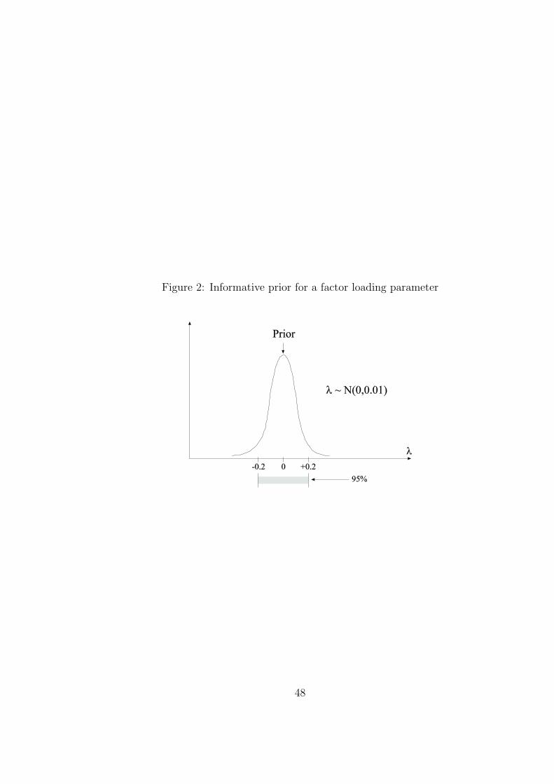
Figure 2: Informative prior for a factor loading parameter

48

List of Tables

1 Choice of variance for a normal prior with mean zero . . . . . . . . . 512 Holzinger-Swineford’s hypothesized four domains measured by 19 tests 523 ML model testing results for Holzinger-Swineford data for Grant-

White (n = 145) and Pasteur (n = 156) . . . . . . . . . . . . . . . . . 534 Holzinger-Swineford ML EFA using 19 variables and Geomin rotation:

Four-factor solution . . . . . . . . . . . . . . . . . . . . . . . . . . . . 545 ML versus Bayes model testing results for Holzinger-Swineford data

for Grant-White (n = 145) and Pasteur (n = 156) . . . . . . . . . . . 556 Bayes for Holzinger-Swineford example: Four-factor solution using

informative priors for cross-loadings . . . . . . . . . . . . . . . . . . . 567 Factor loading pattern for simulation study of cross-loadings . . . . . 578 Bayesian analysis, non-informative cross-loading priors, 0.0 and 0.1

cross-loadings . . . . . . . . . . . . . . . . . . . . . . . . . . . . . . . 589 Rejection rates for ML CFA and Bayes CFA with non-informative priors 5910 ML: cross-loadings 0.0 and 0.1 . . . . . . . . . . . . . . . . . . . . . . 6011 Bayesian analysis using informative, small-variance priors for cross-

loadings 0.0 and 0.1 . . . . . . . . . . . . . . . . . . . . . . . . . . . . 6112 Bayesian analysis using informative, small-variance priors for cross-

loadings 0.2 and 0.3 . . . . . . . . . . . . . . . . . . . . . . . . . . . . 6213 Wording and hypothesized factor loading pattern for the 15 items used

to measure the big-five personality factors in the British HouseholdPanel data (”I see myself as someone who ...”) . . . . . . . . . . . . . 63

14 ML model testing results for big-five personality factors using BritishHousehold Panel data for females (n = 691) and males (n = 589) . . . 64

15 ML exploratory factor analysis of the big-five personality factors usingBritish Household Panel data . . . . . . . . . . . . . . . . . . . . . . 65

16 Bayesian analysis using informative, small-variance priors for residualcorrelations using data for BHPS females and males, Method 2 . . . . 66

17 Rejection rates for ML CFA and Bayes CFA with non-informativepriors for residual covariances . . . . . . . . . . . . . . . . . . . . . . 67

18 Residual correlations =0.1, Method 1 . . . . . . . . . . . . . . . . . . 6819 Residual correlations =0.3, Method 1 . . . . . . . . . . . . . . . . . . 6920 Residual correlations = 0.3, Method 2 and Method 3 . . . . . . . . . 7021 Residual correlations = 0.3, Method 3, freeing the two residual

correlations . . . . . . . . . . . . . . . . . . . . . . . . . . . . . . . . 7122 Antisocial behavior ML EFA . . . . . . . . . . . . . . . . . . . . . . . 7223 Antisocial behavior. BSEM with prior variance = 0.04. Factor solution 7324 Antisocial behavior. BSEM with prior variance = 0.04. Effects of

covariates . . . . . . . . . . . . . . . . . . . . . . . . . . . . . . . . . 74

49

25 Bayesian analysis with informative, small-variance priors for directeffects . . . . . . . . . . . . . . . . . . . . . . . . . . . . . . . . . . . 75

50

Table 1: Choice of variance for a normal prior with mean zero

Variance 90% limits 95% limits

0.001 ±0.05 ±0.060.005 ±0.12 ±0.140.01 ±0.16 ±0.200.02 ±0.23 ±0.280.03 ±0.28 ±0.340.04 ±0.33 ±0.390.05 ±0.37 ±0.440.1 ±0.52 ±0.62

51

Table 2: Holzinger-Swineford’s hypothesized four domains measured by 19 tests

Factor loading pattern

Spatial Verbal Speed Memory

visual X 0 0 0cubes X 0 0 0paper X 0 0 0flags X 0 0 0general 0 X 0 0paragrap 0 X 0 0sentence 0 X 0 0wordc 0 X 0 0wordm 0 X 0 0addition 0 0 X 0code 0 0 X 0counting 0 0 X 0straight 0 0 X 0wordr 0 0 0 Xnumberr 0 0 0 Xfigurer 0 0 0 Xobject 0 0 0 Xnumberf 0 0 0 Xfigurew 0 0 0 X

52

Table 3: ML model testing results for Holzinger-Swineford data for Grant-White (n = 145) andPasteur (n = 156)

Model χ2 df p-value RMSEA CFI

Grant-White

CFA 216 146 0.000 0.057 0.930EFA 110 101 0.248 0.025 0.991

Pasteur

CFA 261 146 0.000 0.071 0.882EFA 128 101 0.036 0.041 0.972

53

Table 4: Holzinger-Swineford ML EFA using 19 variables and Geomin rotation: Four-factorsolution

Loadings

Grant-White PasteurSpatial Verbal Speed Memory Spatial Verbal Speed Memory

visual 0.628* 0.065 0.091 0.085 0.580* 0.307* -0.001 0.053cubes 0.485* 0.050 0.007 -0.003 0.521* 0.027 -0.078 -0.059paper 0.406* 0.107 0.084 0.083 0.484* 0.101 -0.016 -0.229*flags 0.579* 0.160 0.013 0.026 0.687* -0.051 0.067 0.101general 0.042 0.752* 0.126 -0.051 -0.043 0.838* 0.042 -0.118paragrap 0.021 0.804* -0.056 0.098 0.026 0.800* -0.006 0.069sentence -0.039 0.844* 0.085 -0.057 -0.045 0.911* -0.054 -0.029wordc 0.094 0.556* 0.197* 0.019 0.098 0.695* 0.008 0.083wordm 0.004 0.852* -0.074 0.069 0.143* 0.793* 0.029 -0.023addition -0.302* 0.029 0.824* 0.078 -0.247* 0.067 0.664* 0.026code 0.012 0.050 0.479* 0.279* 0.004 0.262* 0.552* 0.082counting 0.045 -0.159 0.826* -0.014 0.073 -0.034 0.656* -0.166straight 0.346* 0.043 0.570* -0.055 0.266* -0.034 0.526* -0.056wordr -0.024 0.117 -0.020 0.523* -0.005 0.020 -0.039 0.726*

numberr 0.069 0.021 -0.026 0.515* -0.026 -0.057 -0.057 0.604*

figurer 0.354* -0.033 -0.077 0.515* 0.329* 0.042 0.168 0.403*

object -0.195 0.045 0.154 0.685* -0.123 -0.005 0.333* 0.469*

numberf 0.225 -0.127 0.246* 0.450* 0.246* 0.092 0.092 0.427*

figurew 0.069 0.099 0.058 0.365* 0.139 0.013 0.237* 0.291*

Factor Correlations


Spatial 1.000 1.000Verbal 0.378* 1.000 0.186* 1.000Speed 0.372* 0.386* 1.000 0.214 0.326* 1.000Memory 0.307* 0.380* 0.375* 1.000 0.190* 0.100 0.242* 1.000

54

Table 5: ML versus Bayes model testing results for Holzinger-Swineford data for Grant-White(n = 145) and Pasteur (n = 156)

ML analysis


Grant-White

CFA 216 146 0.000 0.057 0.930EFA 110 101 0.248 0.025 0.991

Pasteur

CFA 261 146 0.000 0.071 0.882EFA 128 101 0.036 0.041 0.972

Bayesian analysis

Model Sample LRT 2.5% PP limit 97.5% PP limit PP p-value

Grant-White

CFA 219 12 112 0.006CFA w. cross-loadings 160 -31 69 0.242

Pasteur

CFA 264 56 156 0.000CFA w. cross-loadings 175 -13 90 0.068

55

Table 6: Bayes for Holzinger-Swineford example: Four-factor solution using informative priorsfor cross-loadings

Loadings


visual 0.762* -0.022 0.011 0.002 0.710* 0.109 0.015 0.010cubes 0.507* -0.008 -0.014 -0.005 0.479* -0.029 -0.027 -0.020paper 0.489* 0.028 0.032 0.014 0.505* 0.010 -0.023 -0.080flags 0.667* 0.035 -0.024 0.000 0.671* -0.087 0.017 0.062general 0.028 0.778* 0.043 -0.014 -0.052 0.855* 0.018 -0.061paragrap 0.003 0.832* -0.033 0.014 0.022 0.796* -0.002 0.036sentence -0.041 0.867* 0.013 -0.022 -0.058 0.917* -0.021 -0.030wordc 0.048 0.624* 0.082 0.017 0.046 0.698* 0.012 0.051wordm -0.009 0.879* -0.065 0.010 0.074 0.806* 0.002 0.019addition -0.134 0.021 0.782* 0.000 -0.100 -0.010 0.656* -0.001code 0.016 0.052 0.601* 0.049 0.008 0.101 0.665* 0.035counting 0.009 -0.075 0.796* -0.018 0.015 -0.044 0.597* -0.034straight 0.156 0.042 0.629* -0.012 0.098 -0.053 0.557* 0.006wordr -0.027 0.042 -0.010 0.516* -0.040 -0.001 -0.052 0.691*numberr 0.001 -0.002 -0.030 0.543* 0.005 -0.093 -0.067 0.610*figurer 0.102 -0.010 -0.034 0.560* 0.112 0.039 0.042 0.539*object -0.105 0.010 0.021 0.713* -0.067 0.015 0.077 0.550*numberf 0.074 -0.052 0.067 0.584* -0.016 0.039 0.000 0.471*figurew 0.015 0.037 0.003 0.448* 0.032 0.029 0.053 0.417*Factor Correlations


Spatial 1.000 1.000Verbal 0.548* 1.000 0.373* 1.000Speed 0.500* 0.430* 1.000 0.304* 0.445* 1.000Memory 0.557* 0.494* 0.557* 1.000 0.341* 0.163 0.400* 1.000

56

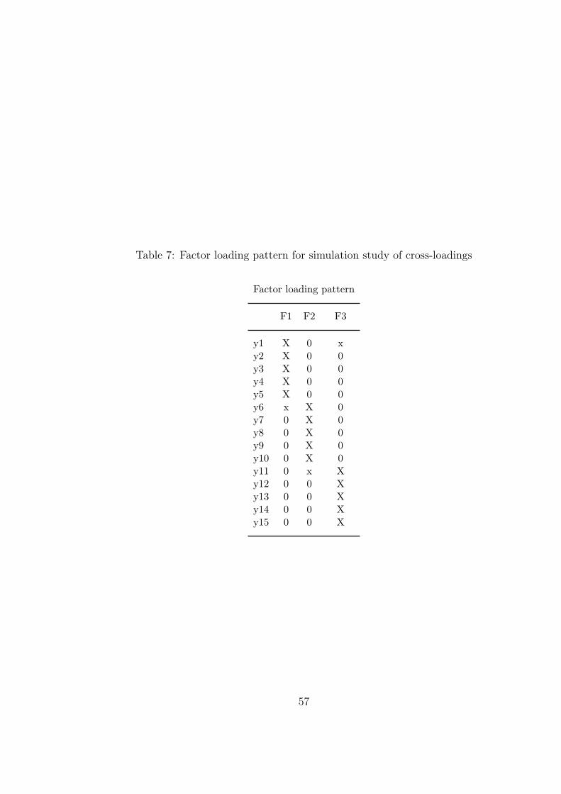
Table 7: Factor loading pattern for simulation study of cross-loadings

Factor loading pattern

F1 F2 F3

y1 X 0 xy2 X 0 0y3 X 0 0y4 X 0 0y5 X 0 0y6 x X 0y7 0 X 0y8 0 X 0y9 0 X 0y10 0 X 0y11 0 x Xy12 0 0 Xy13 0 0 Xy14 0 0 Xy15 0 0 X

57

Table 8: Bayesian analysis, non-informative cross-loading priors, 0.0 and 0.1 cross-loadings

Parameter Estimates S.E. M.S.E. 95% % Sig

Population Average Std. Dev. Average Cover Coeff

Cross-loading = 0.0, n=100, 5% reject proportion for the PPP = 0.036

Major loading 0.800 0.8192 0.1034 0.1005 0.0110 0.928 1.000

Cross-loading 0.000 0.0000 0.0000 0.0000 0.0000 1.000 0.000

Factor variance 1.000 1.0475 0.2447 0.2365 0.0620 0.938 1.000

Factor correlation 0.500 0.5026 0.0872 0.0886 0.0076 0.952 0.996


Major loading 0.800 0.8114 0.0680 0.0677 0.0047 0.948 1.000

Cross-loading 0.000 0.0000 0.0000 0.0000 0.0000 1.000 0.000

Factor variance 1.000 1.0114 0.1635 0.1564 0.0268 0.922 1.000



Major loading 0.800 0.8049 0.0412 0.0415 0.0017 0.946 1.000

Cross-loading 0.000 0.0000 0.0000 0.0000 0.0000 1.000 0.000

Factor variance 1.000 1.0024 0.0974 0.0960 0.0095 0.940 1.000



Major loading 0.800 0.7605 0.0934 0.0905 0.0103 0.902 1.000

Cross-loading 0.000 0.0000 0.0000 0.0000 0.0000 1.000 0.000

Factor variance 1.000 1.2063 0.2713 0.2631 0.1160 0.832 1.000



Major loading 0.800 0.7537 0.0615 0.0612 0.0059 0.860 1.000

Cross-loading 0.000 0.0000 0.0000 0.0000 0.0000 1.000 0.000

Factor variance 1.000 1.1645 0.1796 0.1731 0.0592 0.806 1.000



Major loading 0.800 0.7496 0.0386 0.0374 0.0040 0.700 1.000

Cross-loading 0.000 0.0000 0.0000 0.0000 0.0000 1.000 0.000

Factor variance 1.000 1.1498 0.1092 0.1062 0.0343 0.684 1.000


58

Table 9: Rejection rates for ML CFA and Bayes CFA with non-informative priors

Cross-loading Sample size ML LRT rejection rate Bayes PPP rejection rate

0.0 100 0.172 0.036200 0.090 0.032500 0.060 0.024

0.1 100 0.226 0.056200 0.228 0.080500 0.460 0.262

0.2 100 0.488 0.196200 0.726 0.474500 0.998 0.984

0.3 100 0.830 0.544200 0.996 0.944500 1.000 1.000

59

Table 10: ML: cross-loadings 0.0 and 0.1



Cross-loading = 0.0, n=100, 5% reject proportion for the LRT χ2 test = 0.172

Major loading 0.800 0.8066 0.0984 0.0945 0.0097 0.944 1.000

Cross-loading 0.000 0.0000 0.0000 0.0000 0.0000 1.000 0.000

Factor variance 1.000 0.9842 0.2079 0.2091 0.0435 0.932 1.000



Major loading 0.800 0.8007 0.0667 0.0659 0.0044 0.954 1.000

Cross-loading 0.000 0.0000 0.0000 0.0000 0.0000 1.000 0.000

Factor variance 1.000 0.9870 0.1476 0.1495 0.0219 0.952 1.000



Major loading 0.800 0.8017 0.0420 0.0413 0.0018 0.942 1.000

Cross-loading 0.000 0.0000 0.0000 0.0000 0.0000 1.000 0.000

Factor variance 1.000 0.9970 0.0948 0.0954 0.0090 0.950 1.000



Major loading 0.800 0.7510 0.0894 0.0852 0.0104 0.884 1.000

Cross-loading 0.000 0.0000 0.0000 0.0000 0.0000 1.000 0.000

Factor variance 1.000 1.1281 0.2373 0.2318 0.0726 0.944 1.000



Major loading 0.800 0.7458 0.0606 0.0595 0.0066 0.834 1.000

Cross-loading 0.100 0.0000 0.0000 0.0000 0.0000 1.000 0.000

Factor variance 1.000 1.1316 0.1638 0.1649 0.0441 0.906 1.000



Major loading 0.800 0.7470 0.0381 0.0373 0.0043 0.662 1.000

Cross-loading 0.000 0.0000 0.0000 0.0000 0.0000 1.000 0.000

Factor variance 1.000 1.1430 0.1049 0.1052 0.0314 0.744 1.000


60

Table 11: Bayesian analysis using informative, small-variance priors for cross-loadings 0.0 and0.1




Major loading 0.800 0.8472 0.1212 0.1310 0.0169 0.950 1.000

Cross-loading 0.000 0.0141 0.0455 0.0732 0.0023 0.998 0.002

Factor variance 1.000 0.9864 0.2595 0.2624 0.0674 0.930 1.000



Major loading 0.800 0.8311 0.0893 0.0894 0.0089 0.942 1.000

Cross-loading 0.000 0.0079 0.0421 0.0633 0.0018 1.000 0.000

Factor variance 1.000 0.9662 0.1799 0.1840 0.0335 0.948 1.000



Major loading 0.800 0.8161 0.0520 0.0552 0.0030 0.962 1.000

Cross-loading 0.000 0.0033 0.0313 0.0530 0.0010 1.000 0.000

Factor variance 1.000 0.9741 0.1096 0.1293 0.0127 0.958 1.000



Major loading 0.800 0.8218 0.1177 0.1263 0.0143 0.950 1.000

Cross-loading 0.100 0.0594 0.0449 0.0728 0.0037 0.982 0.038

Factor variance 1.000 1.0600 0.2738 0.2808 0.0784 0.934 1.000



Major loading 0.800 0.8151 0.0860 0.0882 0.0076 0.950 1.000

Cross-loading 0.000 0.0666 0.0424 0.0636 0.0029 0.978 0.098

Factor variance 1.000 1.0217 0.1895 0.1978 0.0363 0.942 1.000



Major loading 0.800 0.8089 0.0517 0.0551 0.0027 0.964 1.000

Cross-loading 0.100 0.0732 0.0316 0.0532 0.0017 0.990 0.176

Factor variance 1.000 1.0169 0.1160 0.1371 0.0137 0.972 1.000


61

Table 12: Bayesian analysis using informative, small-variance priors for cross-loadings 0.2 and0.3




Major loading 0.800 0.7952 0.1152 0.1217 0.0133 0.952 1.000

Cross-loading 0.200 0.1024 0.0453 0.0731 0.0116 0.840 0.188

Factor variance 1.000 1.1522 0.2990 0.3018 0.1124 0.908 1.000



Major loading 0.800 0.7979 0.0835 0.0859 0.0070 0.940 1.000

Cross-loading 0.200 0.1239 0.0418 0.0638 0.0075 0.856 0.492

Factor variance 1.000 1.0850 0.1978 0.2109 0.0463 0.942 1.000



Major loading 0.800 0.8010 0.0514 0.0554 0.0026 0.964 1.000

Cross-loading 0.200 0.1427 0.0327 0.0541 0.0044 0.922 0.854

Factor variance 1.000 1.0595 0.1222 0.1473 0.0184 0.966 1.000



Major loading 0.800 0.7671 0.1104 0.1166 0.0139 0.924 1.000

Cross-loading 0.300 0.1428 0.0460 0.0734 0.0268 0.364 0.470

Factor variance 1.000 1.2532 0.3158 0.3281 0.1636 0.860 1.000



Major loading 0.800 0.7790 0.0807 0.0836 0.0069 0.948 1.000

Cross-loading 0.300 0.1755 0.0419 0.0640 0.0173 0.518 0.856

Factor variance 1.000 1.1623 0.2134 0.2257 0.0718 0.890 1.000



Major loading 0.800 0.7891 0.0493 0.0553 0.0025 0.958 1.000

Cross-loading 0.300 0.2077 0.0318 0.0545 0.0095 0.640 1.000

Factor variance 1.000 1.1116 0.1252 0.1573 0.0281 0.930 1.000


62

Table 13: Wording and hypothesized factor loading pattern for the 15 items used to measurethe big-five personality factors in the British Household Panel data (”I see myself as someonewho ...”)

Agreeableness Conscientiousness Extraversion Neuroticism Openness

y1: Is sometimes rude to others (reverse-scored) X 0 0 0 0y2: Has a forgiving nature X 0 0 0 0y3: Is considerate and kind to almost everyone X 0 0 0 0y4: Does a thorough job 0 X 0 0 0y5: Tends to be lazy (reverse-scored) 0 X 0 0 0y6: Does things efficiently 0 X 0 0 0y7: Is talkative 0 0 X 0 0y8: Is outgoing, sociable 0 0 X 0 0y9: Is reserved (reverse-scored) 0 0 X 0 0y10: Worries a lot 0 0 0 X 0y11: Gets nervous easily 0 0 0 X 0y12: Is relaxed, handles stress well (reverse-scored) 0 0 0 X 0y13: Is original, comes up with new ideas 0 0 0 0 Xy14: Values artistic, aesthetic experiences 0 0 0 0 Xy15: Has an active imagination 0 0 0 0 X

63

Table 14: ML model testing results for big-five personality factors using British Household Paneldata for females (n = 691) and males (n = 589)


Females

CFA 552 80 0.000 0.092 0.795CFA + CUs 432 74 0.000 0.084 0.845EFA 183 40 0.000 0.072 0.938

Males

CFA 516 80 0.000 0.096 0.795CFA + CUs 442 74 0.000 0.092 0.826EFA 113 40 0.000 0.056 0.965

64

Table 15: ML exploratory factor analysis of the big-five personality factors using BritishHousehold Panel data

Loadings

Females MalesF1 F2 Extraver Neurot Open F1 F2 Extraver Neurot Open

y1 0.827* 0.000 0.014 -0.011 -0.005 0.389* 0.010 -0.016 -0.083 -0.294*y2 0.147* 0.215* 0.323* 0.033 0.020 0.188 0.447* 0.123* -0.030 -0.011y3 0.103* 0.569* 0.280* 0.046 -0.095* 0.506* 0.469* 0.026 0.042 -0.030y4 0.018 0.455* -0.003 -0.025 0.270* 0.406* -0.011 0.119* 0.010 0.272*y5 0.365* 0.220* -0.039 -0.068 0.009 0.654* -0.449* -0.037 0.009 0.004y6 -0.016 0.852* 0.001 -0.052 0.087 0.656* 0.077 0.020 -0.090 0.141*y7 -0.154* 0.053 0.541* 0.015 0.129* 0.047 0.015 0.629* 0.045 0.123y8 -0.041 -0.024 0.748* -0.049 -0.002 0.012 0.024 0.795* -0.051 0.032y9 0.064 -0.416* 0.346* -0.116* 0.031 -0.156 -0.380* 0.396* -0.010 -0.049y10 -0.045 0.061 0.063 0.727* 0.036 0.023 0.020 -0.029 0.698* 0.294*y11 0.021 0.001 -0.039 0.670* 0.013 -0.075 0.279* -0.052 0.519* 0.021y12 0.022 -0.250* -0.061 0.547* -0.063 -0.004 -0.311* 0.051 0.648* -0.109y13 0.024 0.011 -0.036 -0.107 0.764* 0.069 -0.007 -0.001 -0.023 0.734*

y14 0.011 -0.088* 0.038 0.125* 0.659* -0.073 0.057 0.035 0.036 0.486*

y15 -0.054 0.140* 0.087 -0.014 0.541* 0.002 0.006 0.038 -0.146* 0.671*

Factor correlations

Females MalesF1 F2 Extraver Neurot Open F1 F2 Extraver Neurot Open

F1 1.000 1.000F2 0.151* 1.000 0.399* 1.000Extraver -0.024 0.362* 1.000 0.268* 0.200* 1.000Neurot -0.085 0.100* -0.108* 1.000 -0.311* 0.065 -0.252* 1.000Open -0.142* 0.229* 0.473* -0.175* 1.000 0.344* 0.397* 0.454* -0.180* 1.000

65

Table 16: Bayesian analysis using informative, small-variance priors for residual correlationsusing data for BHPS females and males, Method 2

Loadings

Females MalesAgreeab Conscien Extraver Neurot Open Agreeab Conscien Extraver Neurot Open

y1 0.772* -0.006 -0.026 0.000 -0.012 0.842* -0.013 -0.011 -0.010 -0.018y2 0.575 -0.014 0.021 -0.013 0.028 0.394 -0.006 0.024 -0.006 0.018y3 0.503* 0.034 0.023 0.012 -0.010 0.479* 0.040 0.005 0.021 0.013y4 -0.029 0.704* 0.014 -0.003 0.024 -0.040 0.683* 0.027 0.019 0.017y5 0.017 0.657* -0.001 0.006 -0.028 0.014 0.708* -0.020 0.002 -0.018y6 0.032 0.548* -0.015 -0.007 0.015 0.043 0.579* 0.000 -0.036 0.007y7 -0.008 0.014 0.685* 0.024 0.006 -0.005 0.005 0.748* 0.016 -0.005y8 0.023 0.002 0.702* -0.017 0.003 0.024 0.011 0.754* -0.023 0.013y9 -0.016 -0.021 0.622* -0.008 0.002 -0.025 -0.015 0.575* 0.005 -0.005y10 -0.003 0.025 0.022 0.791* 0.023 0.001 0.009 0.013 0.801* 0.044y11 0.016 -0.007 -0.024 0.736* -0.008 0.012 -0.010 -0.022 0.708* -0.024y12 -0.012 -0.022 -0.004 0.695* -0.027 -0.017 -0.006 0.003 0.613* -0.034y13 0.006 0.020 0.006 -0.047 0.780* 0.004 0.023 -0.008 0.007 0.732*

y14 -0.008 -0.010 -0.007 0.046 0.738* 0.004 -0.021 -0.013 0.023 0.672*

y15 0.006 -0.006 0.011 -0.003 0.660* -0.011 0.001 0.031 -0.035 0.651*

Factor correlations

Females MalesAgreeab Conscien Extraver Neurot Open Agreeab Conscien Extraver Neurot Open

Agreeab 1.000 1.000Conscien 0.366* 1.000 0.319* 1.000Extraver 0.081 0.119 1.000 0.025 0.197 1.000Neurot -0.059 -0.093 -0.163 1.000 -0.133 -0.238* -0.160 1.000Open 0.041 0.201 0.321* -0.158 1.000 0.040 0.250 0.297* -0.091 1.000

66

Table 17: Rejection rates for ML CFA and Bayes CFA with non-informative priors for residualcovariances

Cross-loading Sample size ML LRT rejection rate Bayes PPP rejection rate

0.0 200 0.048 0.024500 0.070 0.024

0.1 200 0.750 0.510500 1.000 0.984

0.3 200 1.000 1.000500 1.000 1.000

67

Table 18: Residual correlations =0.1, Method 1



Residual covariance = 0.1, df=30, n=200, 5% reject proportion for the PPP = 0.024

Factor loading 0.800 0.8074 0.0690 0.0688 0.0048 0.942 1.000

Residual covariance 0.100 0.0154 0.0106 0.0159 0.0073 0.044 0.076

Factor variance 1.000 1.0257 0.1602 0.1595 0.0263 0.934 1.000



Factor loading 0.800 0.8035 0.0425 0.0449 0.0018 0.958 1.000


Factor variance 1.000 1.0296 0.1010 0.1016 0.0111 0.946 1.000



Factor loading 0.800 0.8103 0.0694 0.0792 0.0049 0.970 1.000


Factor variance 1.000 1.0139 0.1596 0.1717 0.0256 0.952 1.000



Factor loading 0.800 0.8056 0.0447 0.0552 0.0020 0.976 1.000


Factor variance 1.000 1.0142 0.1015 0.1148 0.0105 0.968 1.000


68

Table 19: Residual correlations =0.3, Method 1




Factor loading 0.800 0.8041 0.0401 0.0437 0.0016 0.970 1.000


Factor variance 1.000 1.1252 0.1425 0.1464 0.0359 0.864 1.000



Factor loading 0.800 0.8029 0.0264 0.0293 0.0007 0.962 1.000


Factor variance 1.000 1.0855 0.0901 0.0933 0.0154 0.850 1.000



Factor loading 0.800 0.8058 0.0411 0.0494 0.0017 0.974 1.000


Factor variance 1.000 1.0461 0.1424 0.1554 0.0224 0.948 1.000



Factor loading 0.800 0.8033 0.0278 0.0347 0.0008 0.986 1.000


Factor variance 1.000 1.0199 0.0930 0.1042 0.0090 0.972 1.000


69

Table 20: Residual correlations = 0.3, Method 2 and Method 3



Method 2, residual covariance = 0.3, df = 30, n=200

Factor loading 0.800 0.8041 0.0402 0.0431 0.0016 0.958 1.000


Factor variance 1.000 0.9809 0.1349 0.1429 0.0185 0.946 1.000


Method 2, residual covariance = 0.3, df = 30, n=500

Factor loading 0.800 0.8029 0.0260 0.0311 0.0007 0.972 1.000


Factor variance 1.000 0.9541 0.0865 0.1016 0.0096 0.952 1.000


Method 3, residual covariance = 0.3, V = 0.001, n=200

Factor loading 0.800 0.8076 0.0536 0.0587 0.0029 0.970 1.000


Factor variance 1.000 1.0550 0.1482 0.1529 0.0249 0.928 1.000


Method 3, residual covariance = 0.3, V = 0.001, n=500

Factor loading 0.800 0.8047 0.0379 0.0456 0.0015 0.980 1.000


Factor variance 1.000 1.0390 0.0964 0.1039 0.0108 0.956 1.000


70

Table 21: Residual correlations = 0.3, Method 3, freeing the two residual correlations



Residual correlations = 0.3, V = 0.001, freeing the two residual correlations, n=200

Factor loading 0.800 0.8074 0.0463 0.0599 0.0022 0.988 1.000


Factor variance 1.000 0.9959 0.1358 0.1494 0.0184 0.966 1.000


Residual correlations = 0.3, V = 0.001, freeing the two residual correlations, n=500

Factor loading 0.800 0.8074 0.0462 0.0600 0.0022 0.992 1.000


Factor variance 1.000 0.9965 0.1354 0.1495 0.0183 0.968 1.000


71

Table 22: Antisocial behavior ML EFA

Parameter Prop Person Drugs

property 0.736* 0.118* -0.061fight 0.267* 0.497* -0.047shoplift 0.645* -0.076 0.151*lt50 0.830* -0.196* 0.003gt50 0.824* -0.013 0.002force 0.420* 0.341* 0.011threat 0.018 0.772* 0.163injure -0.012 0.740* 0.199*pot -0.034 -0.013 0.908*drug 0.018 -0.044 0.872*soldpot 0.162* 0.015 0.758*solddrug 0.174* 0.012 0.689*con 0.484* 0.191* -0.059auto 0.493* 0.118* 0.081bldg 0.844* -0.015 -0.003goods 0.732* 0.072 0.061gambling 0.372* 0.332* 0.119

Factor correlations

Prop Person Drugs

prop 1.000person 0.564 1.000drugs 0.629 0.256 1.000

72

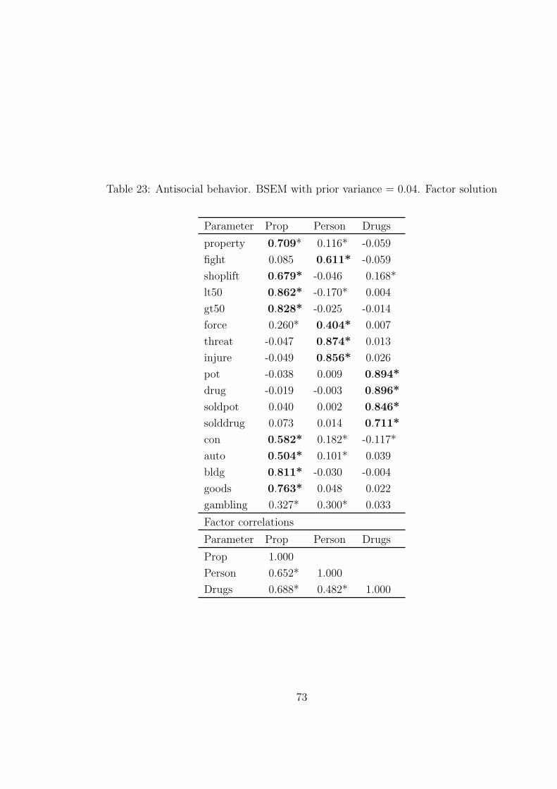
Table 23: Antisocial behavior. BSEM with prior variance = 0.04. Factor solution


property 0.709* 0.116* -0.059

fight 0.085 0.611* -0.059

shoplift 0.679* -0.046 0.168*

lt50 0.862* -0.170* 0.004

gt50 0.828* -0.025 -0.014

force 0.260* 0.404* 0.007

threat -0.047 0.874* 0.013

injure -0.049 0.856* 0.026

pot -0.038 0.009 0.894*

drug -0.019 -0.003 0.896*

soldpot 0.040 0.002 0.846*

solddrug 0.073 0.014 0.711*

con 0.582* 0.182* -0.117*

auto 0.504* 0.101* 0.039

bldg 0.811* -0.030 -0.004

goods 0.763* 0.048 0.022

gambling 0.327* 0.300* 0.033

Factor correlations


Prop 1.000

Person 0.652* 1.000

Drugs 0.688* 0.482* 1.000

73

Table 24: Antisocial behavior. BSEM with prior variance = 0.04. Effects of covariates

Parameter Age94 Male Black

Factors

prop -0.164 0.361* -0.032

person -0.104 0.333* 0.119*

drugs 0.093 0.133* -0.139*

Items

property -0.055 0.028 -0.051*

fight -0.142 0.107* 0.052*

shoplift -0.029 -0.144* 0.017

lt50 0.093 -0.031 -0.048

gt50 0.078 0.013 0.066*

force 0.002 0.025 0.114*

threat -0.056 -0.013 -0.066

injure 0.017 -0.053 0.007

pot 0.033 -0.028 0.029

drug 0.031 -0.051 -0.074*

soldpot -0.067 0.085* 0.024

solddrug -0.012 0.015 0.061

con -0.019 -0.140* 0.075*

auto -0.042 -0.048 -0.029

bldg 0.027 0.082* -0.040

goods 0.049 0.022 -0.018

gambling 0.089 0.077* 0.033

74

Table 25: Bayesian analysis with informative, small-variance priors for direct effects



Direct effect = 0.4, n=500, 5% reject proportion for the PPP = 0.000

Major loading 1.000 1.0981 0.2030 0.2009 0.0508 0.930 1.000

Factor slope on X 0.500 0.5277 0.1265 0.1489 0.0167 0.974 0.994

Direct effect of Y on X 0.400 0.2456 0.0850 0.1328 0.0310 0.884 0.422

Factor residual variance 1.000 0.9065 0.2539 0.2371 0.0731 0.892 1.000

Factor residual correlation 0.500 0.5066 0.0530 0.0557 0.0028 0.952 1.000


Major loading 1.000 1.0462 0.1360 0.1357 0.0206 0.950 1.000

Factor slope on X 0.500 0.5602 0.1000 0.1242 0.0136 0.958 1.000





Major loading 1.000 1.0220 0.0955 0.0937 0.0096 0.942 1.000

Factor slope on X 0.500 0.5676 0.0730 0.1061 0.0099 0.972 1.000




75

Bayesian SEM: A more flexible representation of substantive theory

Documents

Transcript of Bayesian SEM: A more flexible representation of substantive theory