Bayesian Reliability Testing for New Generation Semiconductor...
32
5/21/2003 0 2003 QPRC 2003 QPRC: Bayesian Reliability Testing for New Generation Semiconductor Processing Equipment Bayesian Reliability Testing for New Generation Semiconductor Processing Equipment Paul Tobias and Michael Pore CONTENTS A. Review of Classical Approach for Planning an Equipment Reliability Qualification Test B. What If It Takes Too Long Or Costs Too Much? C. What is the Bayesian Approach? D. How to Use Old Test Data and/or Engineering Judgment to Specify the Gamma Prior and Determine the Needed Test Time E. Summary F. References
Transcript of Bayesian Reliability Testing for New Generation Semiconductor...

5/21/2003 0 2003 QPRC
2003 QPRC: Bayesian Reliability Testing for New Generation Semiconductor Processing Equipment
Bayesian Reliability Testing for New Generation Semiconductor Processing Equipment
Paul Tobias and Michael Pore
CONTENTSA. Review of Classical Approach for Planning an Equipment
Reliability Qualification Test
B. What If It Takes Too Long Or Costs Too Much?
C. What is the Bayesian Approach?
D. How to Use Old Test Data and/or Engineering Judgment to Specify the Gamma Prior and Determine the Needed Test Time
E. Summary
F. References

5/21/2003 1 2003 QPRC
2003 QPRC: Bayesian Reliability Testing for New Generation Semiconductor Processing Equipment
A. Review of Classical Approach for Planning an Equipment Reliability Qualification Test
(Follows Reference 3, also in Reference 2,4)
Goal: We want to measure a new tool’s performance for a “qualification” period and assure it meets specified reliabilityrequirements.Question: How long a test period is needed - assuming an Exponential Model or constant repair rate (HPP) - no trends or reliability “growth” or “degradation”?
i) We first specify a Mean Time Between Failures (MTBF) objective and a confidence level we want to have that the tool will actually meet that objective during its useful life.
ii) Next we pick a trial number of failures we would like to allow to occur and still pass the acceptance test. We can iterate several times on this choice, with 4 often recommended as a typical starting point and 0 used for minimum test time plans.

5/21/2003 2 2003 QPRC
2003 QPRC: Bayesian Reliability Testing for New Generation Semiconductor Processing Equipment
iii) Using the “Test Length Table” we find a factor to multiply the MTBF objective with in order to obtain the needed test time.
iv) When the test is complete, we calculate the demonstrated MTBF and multiply by the appropriate factor from the “Lower Limit Confidence Bound Table” to determine the actual MTBF confirmed by the test

5/21/2003 3 2003 QPRC
2003 QPRC: Bayesian Reliability Testing for New Generation Semiconductor Processing Equipment
TEST LENGTH TABLE
NUMBER OF
FAILURES
k FACTOR FOR GIVEN CONFIDENCE LEVELS
r 50% 60% 75% 80% 90% 95%
0 .693 .916 1.39 1.61 2.30 3.00
1 1.68 2.02 2.69 2.99 3.89 4.74
2 2.67 3.11 3.92 4.28 5.32 6.30
3 3.67 4.18 5.11 5.52 6.68 7.75
4 4.67 5.24 6.27 6.72 7.99 9.15
5 5.67 6.29 7.42 7.90 9.28 10.51
6 6.67 7.35 8.56 9.07 10.53 11.84
7 7.67 8.38 9.68 10.23 11.77 13.15
8 8.67 9.43 10.80 11.38 13.00 14.43
9 9.67 10.48 11.91 12.52 14.21 15.70
10 10.67 11.52 13.02 13.65 15.40 16.96
15 15.67 16.69 18.48 19.23 21.29 23.10
20 20.68 21.84 23.88 24.73 29.06 30.89
Use to determine the test time needed to demonstrate a desired MTBFp at a given confidence level if r failures occur. Multiply the desired MTBFp by the k factor corresponding to r and the confidence level.
5/21/2003 4 2003 QPRC
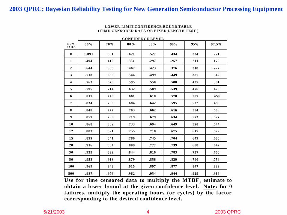
2003 QPRC: Bayesian Reliability Testing for New Generation Semiconductor Processing Equipment
LOWER LIMIT CONFIDENCE BOUND TABLE (TIME-CENSORED DATA OR FIXED LENGTH TEST )
CONFIDENCE LEVEL
N U M . FAILS
60% 70% 80% 85% 90% 95% 97.5%
0 1.091 .831 .621 .527 .434 .334 .271
1 .494 .410 .334 .297 .257 .211 .179
2 .644 .553 .467 .423 .376 .318 .277
3 .718 .630 .544 .499 .449 .387 .342
4 .763 .679 .595 .550 .500 .437 .391
5 .795 .714 .632 .589 .539 .476 .429
6 .817 .740 .661 .618 .570 .507 .459
7 .834 .760 .684 .642 .595 .532 .485
8 .848 .777 .703 .662 .616 .554 .508
9 .859 .790 .719 .679 .634 .573 .527
10 .868 .802 .733 .694 .649 .590 .544
12 .883 .821 .755 .718 .675 .617 .572
15 .899 .841 .780 .745 .704 .649 .606
20 .916 .864 .809 .777 .739 .688 .647
30 .935 .892 .844 .816 .783 .737 .700
50 .953 .918 .879 .856 .829 .790 .759
100 .969 .943 .915 .897 .877 .847 .822
500 .987 .976 .962 .954 .944 .929 .916
Use for time censored data to multiply the MTBF p estimate to obtain a lower bound at the given confidence level. Note: for 0 failures, multiply the operating hours (or cycles) by the factor corresponding to the desired confidence level.

5/21/2003 5 2003 QPRC
2003 QPRC: Bayesian Reliability Testing for New Generation Semiconductor Processing Equipment
ExampleAssume you want to verify a new prototype tool’s MTBF is at least 300 hours at 80% confidence.
– Using the Test Length Table , you plan a test for 6.72x300 = 2016 hours = 12 weeks
» If you have no more than 4 failures you have confirmed an MTBF of at least 300 hours with 80% confidence
– If you run the test and have only 3 failures» The MTBF point estimate is 2016/3 = 672 and an 80% lower bound
(using the factor .544 from the Lower Limit Confidence Bound Table) is 672x.544 = 366 hours
But what if you only have time (or money) for a two week test (336 hours) and there is only one prototype tool available to test? Even the “0” failures factor of 1.61 leads to a required test time of 483 hours with no failures allowed. Are there any other “legitimate” options available?

5/21/2003 6 2003 QPRC
2003 QPRC: Bayesian Reliability Testing for New Generation Semiconductor Processing Equipment
B. What If It Takes Too Long Or Costs Too Much?
• New generations of technology come along every few years– Hundreds of new multi-million dollar tools need to be qualified rapidly– First pass Reliability Qualification often occurs early, when only a
prototype tool exists– Test materials (silicon wafers) are often expensive and in short supply
• At the same time, productivity requirements are driving a need for higher and higher Tool MTBF’s
• International SEMATECH faced this situation when its member companies asked it to look prototypes of new, 300mm wafer processing tools

5/21/2003 7 2003 QPRC
2003 QPRC: Bayesian Reliability Testing for New Generation Semiconductor Processing Equipment
• When classical Reliability Qualification Tests take too long and cost too much other methods are needed
• This is a good situation to apply Bayesian methods since– Many new tools are very similar to older tools that
engineers have a good deal of data and experience evaluating
– Supplier test data and/or sub assembly test data is often available
– Making use of prior knowledge and experience, as well as engineering judgment “makes sense” to engineers – they are quick to accept the Bayesian Paradigm
5/21/2003 8 2003 QPRC
2003 QPRC: Bayesian Reliability Testing for New Generation Semiconductor Processing Equipment
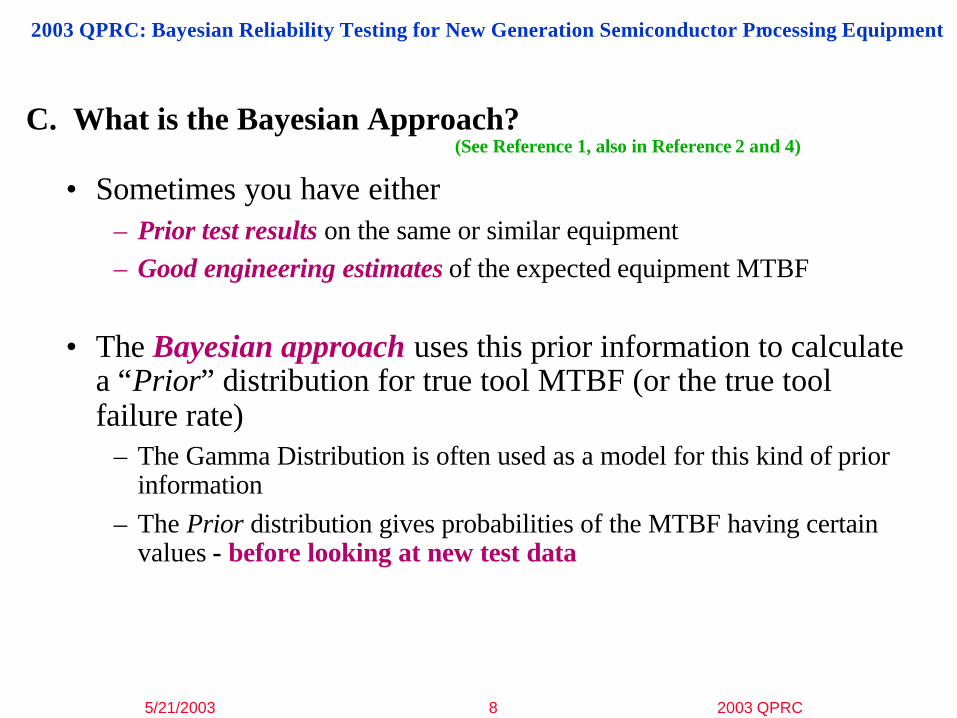
C. What is the Bayesian Approach?(See Reference 1, also in Reference 2 and 4)
• Sometimes you have either– Prior test results on the same or similar equipment– Good engineering estimates of the expected equipment MTBF
• The Bayesian approach uses this prior information to calculate a “Prior” distribution for true tool MTBF (or the true tool failure rate)
– The Gamma Distribution is often used as a model for this kind of prior information
– The Prior distribution gives probabilities of the MTBF having certain values - before looking at new test data

5/21/2003 9 2003 QPRC
2003 QPRC: Bayesian Reliability Testing for New Generation Semiconductor Processing Equipment
• Then, data from a new test is used to “update” this Priordistribution into a “Posterior” distribution
– The Posterior distribution will also be Gamma when the constant failure rate (exponential distribution) assumption applies – the Gamma is the Conjugate Prior
– The Posterior distribution gives updated probabilities that the MTBF lies in a given range of values

5/21/2003 10 2003 QPRC
2003 QPRC: Bayesian Reliability Testing for New Generation Semiconductor Processing Equipment
• Either the mean or the 50% (median) point of the posterior gamma distribution can be used as the MTBF estimate
– The 10 or 20% point of this distribution is a lower bound on the MTBF
– Probability intervals of all kinds can be constructed from the posterior distribution.
5/21/2003 11 2003 QPRC
2003 QPRC: Bayesian Reliability Testing for New Generation Semiconductor Processing Equipment
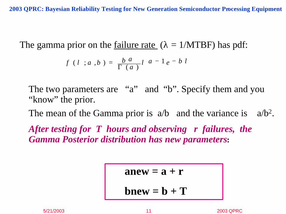
The gamma prior on the failure rate (λ = 1/MTBF) has pdf:
The two parameters are “a” and “b”. Specify them and you “know” the prior. The mean of the Gamma prior is a/b and the variance is a/b2.
After testing for T hours and observing r failures, the Gamma Posterior distribution has new parameters:
f a b b aa
a e b( ; , )( )
λ λ λ= − −Γ
1
anew = a + r
bnew = b + T

5/21/2003 12 2003 QPRC
2003 QPRC: Bayesian Reliability Testing for New Generation Semiconductor Processing Equipment
How the “Prior” Model Becomes the “Posterior” Model
0
5
10
15
20
25
30
0 50 100 150 200 250 300 350 400 450 500
MTBF
PD
F
New Data:(r fails, T time on test)
0
10
20
30
40
50
60
70
80
90
0 5 0 100 150 200 250 300 350 400 450 500
MTBF
PD
F
Gamma prior
Exponential Data ModelGamma Posterior
G(a, b)
exp(λ)G(anew, bnew)
anew = a + rbnew = b + T

5/21/2003 13 2003 QPRC
2003 QPRC: Bayesian Reliability Testing for New Generation Semiconductor Processing Equipment
EXCEL can be used to easily evaluate Bayesian test results (or evaluate the Posterior distribution) with the built in function GAMMAINV.
1/GAMMAINV (1- α, anew, 1/bnew)
will return the value MTBFlower where the lower bound is at 100 x (1- α) confidence.

5/21/2003 14 2003 QPRC
2003 QPRC: Bayesian Reliability Testing for New Generation Semiconductor Processing Equipment
A 100x(1 - α) lower bound for the MTBF after the test can also be evaluated using Chi Square tables as:
2bnew/χ22anew;1-α
CAUTION: If using EXCEL to evaluate the Chi Square distribution, only integer values of “anew” will give correct answers. But EXCEL will correctly evaluate the Gamma for all parameter values (EXCEL uses beta = 1/b for its second parameter)

5/21/2003 15 2003 QPRC
2003 QPRC: Bayesian Reliability Testing for New Generation Semiconductor Processing Equipment
• Past “knowledge” came from the engineers who were experts for the prototype tool and typically took the form of
1. Actual previous test data on the same or similar equipment (this data was often “weighted” for credibility by applying a factor between 0 and 1 to the test time and the observed fails)
or 2. Entering a “best” starting guess for the MTBF (a 50% value) and a
low value the engineers were (95%) confident the MTBF would exceed
• These starting guesses were the consensus of a group of experts (sometimes called the “Socratic” approach to obtaining a prior)
D. How to Use Old Test Data and/or Engineering Judgment to Specify the Gamma Prior and Determine the Needed Test Time

5/21/2003 16 2003 QPRC
2003 QPRC: Bayesian Reliability Testing for New Generation Semiconductor Processing Equipment
If we have actual past data that can be accepted as applicable (best possible case!): say “a” failures in “b” hours of past test data - use these for the parameters for the Gamma prior.
To plan a Test to confirm an MTBF of M at 80% confidence, while allowing up to r failures using EXCEL
set M = 1/GAMMINV(.8, a + r, 1/[b + T])
and try values of T until the right side does equal M.
That value of T is the new test time. Or, use the built in EXCEL “GOAL SEEK” function to quickly find T.

5/21/2003 17 2003 QPRC
2003 QPRC: Bayesian Reliability Testing for New Generation Semiconductor Processing Equipment
Example 1 Previous testing on a new tool had 11 failures in 1400 hours. However, 10 of these failures were due to the same poorly designed mechanical arm. A new arm assembly has replaced the old and the new arm has a proven history of reliable operation with an MTBF in excess of 10,000 hours.
The goal is to confirm a tool MTBF of 500 hours at 80% confidence.
A consensus is reached that, with the new arm, most likely none of the mechanical arm failures would have occurred - but surely no more than one. So prior data of 2 failures in 1400 hours is accepted as reasonable for the redesigned tool.

5/21/2003 18 2003 QPRC
2003 QPRC: Bayesian Reliability Testing for New Generation Semiconductor Processing Equipment
Example 1: Continued
The assumed prior data is: 2 failures in 1400 hours and the Gamma prior therefore has parameters a = 2, b = 1400.
If we want to allow up to 2 failures on the qualification test we can use EXCEL to solve for T using
500 = 1/GAMMAINV(.8, 4, 1/(1400 + T))
The solution is T = 1358 hours.
The step by step procedure, using GOAL SEEK, follows.
5/21/2003 19 2003 QPRC
2003 QPRC: Bayesian Reliability Testing for New Generation Semiconductor Processing Equipment
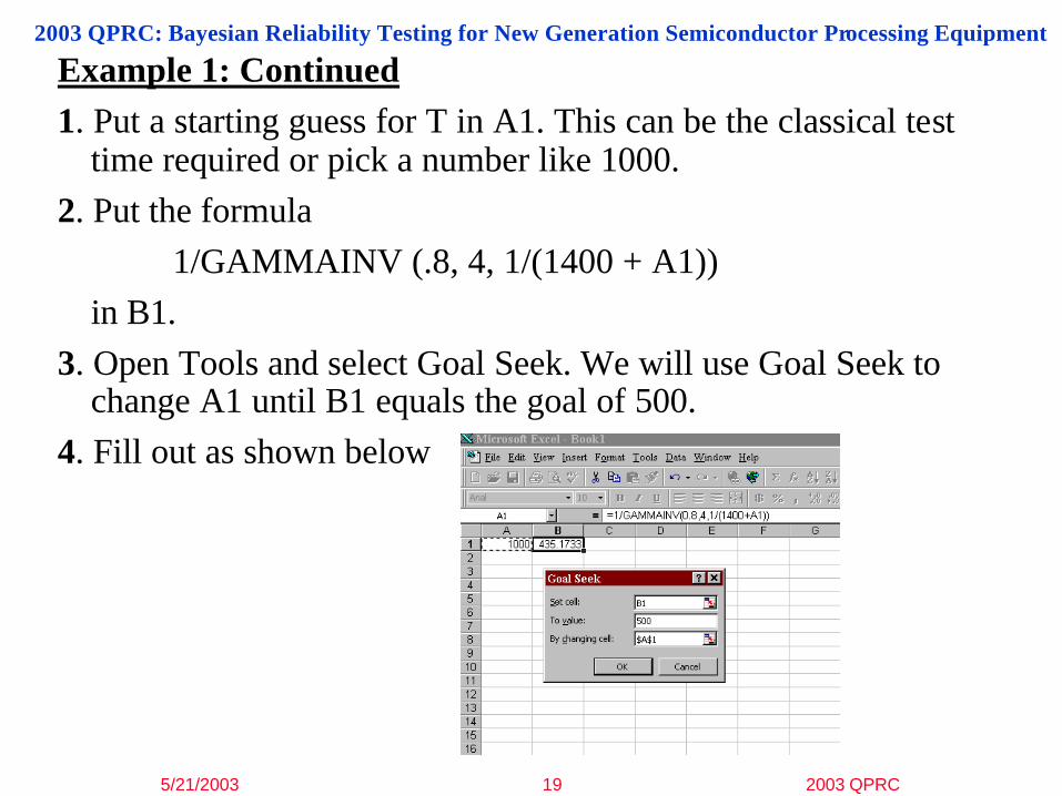
Example 1: Continued1. Put a starting guess for T in A1. This can be the classical test
time required or pick a number like 1000.2. Put the formula
1/GAMMAINV (.8, 4, 1/(1400 + A1))in B1.
3. Open Tools and select Goal Seek. We will use Goal Seek to change A1 until B1 equals the goal of 500.
4. Fill out as shown below

5/21/2003 20 2003 QPRC
2003 QPRC: Bayesian Reliability Testing for New Generation Semiconductor Processing Equipment
Example 1: Continued
5. Hit OK and watch as A1 changes to the required test time of 1357.5 (or 1358) hours.
6. If you test for 1358 hours and have no more than 2 failures, you will have confirmed a goal of a MTBF of at least 500 hours.
5/21/2003 21 2003 QPRC
2003 QPRC: Bayesian Reliability Testing for New Generation Semiconductor Processing Equipment
Example 1: Continued
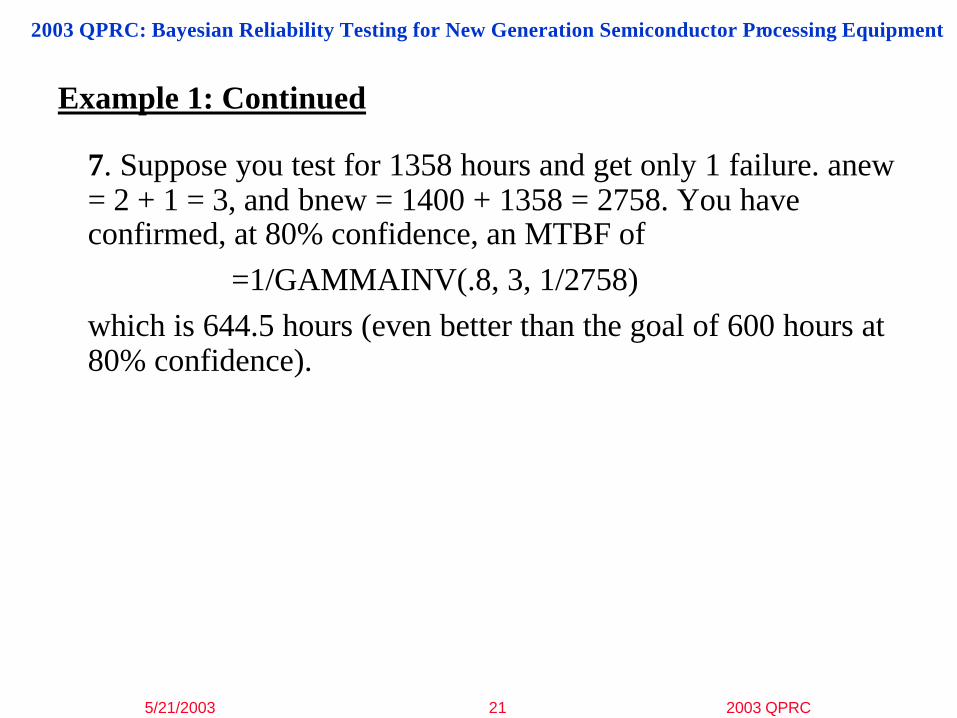
7. Suppose you test for 1358 hours and get only 1 failure. anew = 2 + 1 = 3, and bnew = 1400 + 1358 = 2758. You have confirmed, at 80% confidence, an MTBF of
=1/GAMMAINV(.8, 3, 1/2758)which is 644.5 hours (even better than the goal of 600 hours at 80% confidence).

5/21/2003 22 2003 QPRC
2003 QPRC: Bayesian Reliability Testing for New Generation Semiconductor Processing Equipment
Example 2 (Socratic Method)Instead of actual old data, we have a consensus engineering judgement (average or median “best guess”) for the MTBF.We put this as our “50%” estimate. We next agree upon a low MTBF value that engineers are 90 or 95% confident the new tool will exceed (i.e. we would “bet” 9 to1 or 19 to 1 that the true MTBF is better than this value).
These 2 MTBF values can be used to derive prior parameters “a” and “b” - since only one gamma prior passes through these percentile points. Once we have “a” and “b”, a test time is calculated as in Example 1.NOTE: We can pick any two percentiles and the more conservative we are, the more readily the resulting analysis will be accepted
Use of EXCEL to obtain a and b follows next

5/21/2003 23 2003 QPRC
2003 QPRC: Bayesian Reliability Testing for New Generation Semiconductor Processing Equipment
Example 2: Continued
The consensus is the MTBF is equally likely to be above 500 hours as below. It is also considered highly unlikely that the MTBF will be as low as 100 hours. The value 100 is considered to be a 95% lower limit for the MTBF, prior to testing.
This information used to derive the “a” and “b” parameters of a Gamma prior as follows:
1. Calculate the ratio of the two MTBF’s:R = 500/100 = 5
2. Open an EXCEL spreadsheet and put a starting value of 1 in A1
3. Put=(GAMMAINV(0.95,A1,1))/GAMMAINV(0.5,A1,1)
in B1

5/21/2003 24 2003 QPRC
2003 QPRC: Bayesian Reliability Testing for New Generation Semiconductor Processing Equipment
Example 2: Continued
4. Open Goal Seek from the Tools button and put B1 in “Set Cell”,the ratio R = 5 in “To Value” and $A$1 in “By Changing Cell”
5/21/2003 25 2003 QPRC
2003 QPRC: Bayesian Reliability Testing for New Generation Semiconductor Processing Equipment
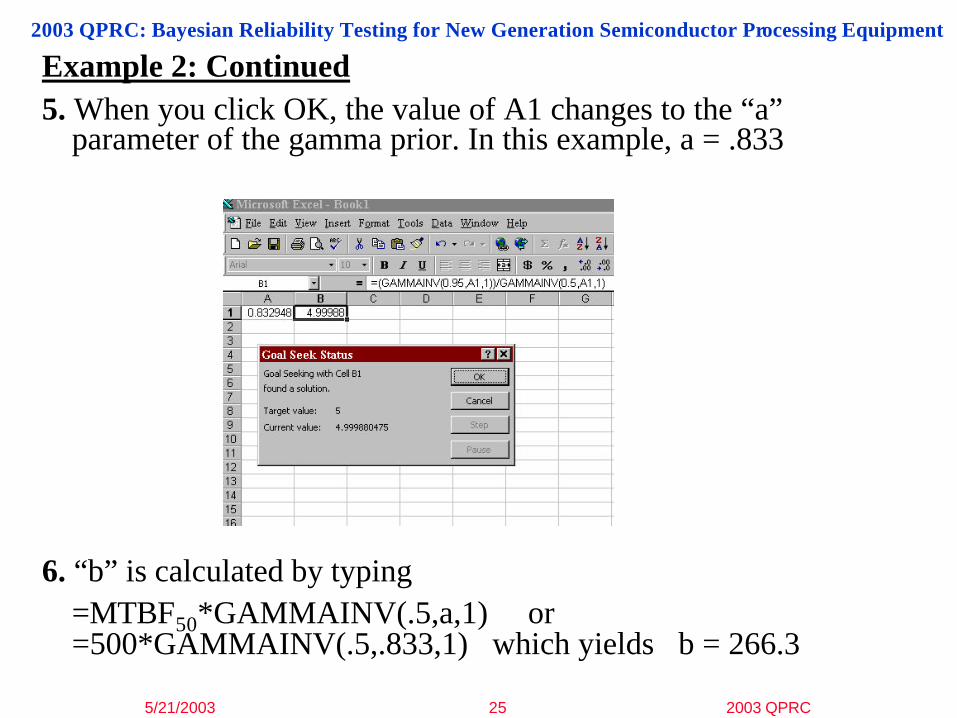
Example 2: Continued5. When you click OK, the value of A1 changes to the “a”
parameter of the gamma prior. In this example, a = .833
6. “b” is calculated by typing =MTBF50*GAMMAINV(.5,a,1) or =500*GAMMAINV(.5,.833,1) which yields b = 266.3

5/21/2003 26 2003 QPRC
2003 QPRC: Bayesian Reliability Testing for New Generation Semiconductor Processing Equipment
Using Historical Data• Sometimes tests have been performed by others and you may
or may not wish to give them the same “value” as current tests.• We refer to these previous tests as historical data.• Historical data may be weighted.
* Using it may reduce required test times.* The influence of such data is reduced to reflect the perceived
reliability of the source
• The weighting is a number w, 0 < w < 1, reflecting the proportion of influence we want the historical data to have
• The situation looks as follows:(a, b) = parameters of a (starting) prior gamma distribution(adata, bdata) = fails & time of the historical data(r, T) = fails & time of the current test
• The posterior parameters areanew = a + (adata*w) + rbnew = b + (bdata*w) + T

5/21/2003 27 2003 QPRC
2003 QPRC: Bayesian Reliability Testing for New Generation Semiconductor Processing Equipment
The Non-Informative Prior Is A Common “Starting” Prior
• The prior distribution that reflects no knowledge or experience about the MTBF is the gamma distribution with a = 0 (no previous failure data) and b= 0 (no previous test time): this gamma (0, 0) – it is called a Non-Informative Prior
• It is easy to see that gamma (0,0) is the function f(λ) = 1/λ
• Gamma (0, 0) is an improper probability distribution (isn’t a real CDF – it integrates to infinity), but when analyzed with data (with r > 0 and T > 0) it produces a proper posterior gamma distribution.
• This non-informative prior will yield a posterior that gives exactly the same results as the classical analysis will.
* However, when the test yields r = 0, the Bayesian with gamma (0, 0) does not work.
5/21/2003 28 2003 QPRC
2003 QPRC: Bayesian Reliability Testing for New Generation Semiconductor Processing Equipment
When to Use Bayesian Analysis / When Not
• When anew = a + (adata*w) + r = 0, use the classical special case analysis or use a “more informative” prior (i.e., with a > 0).
• All other cases admit to Bayesian analyses– It is often easier to “sell” a “less informative” prior, especially when little
is known about the reliability of the new system under analysis. The gamma (0, 0) is the most non-informative prior and will yield classical analysis results.
• When you wish to use all the available data (expert opinion, previous tests, and/or historical data) then put together all the prior data that reflects the current state-of-knowledge about the MTBF and proceed with a Bayesian analysis!

5/21/2003 29 2003 QPRC
2003 QPRC: Bayesian Reliability Testing for New Generation Semiconductor Processing Equipment
E. Summary
• When the goal is to establish the reliability level with as little risk as possible and there is enough time and/or materials available -use classical methods or Bayesian with the non-informative prior.
• When the goal is to confirm as much as possible in a short time (and the increased risk of using either old data or engineering judgement is acceptable) consider using other Bayesian Methods –remember that a more non-informative prior is easier for many people to accept.
• Remember the “drawbacks”– Unlike the “classical” approach, the results do not stand by themselves– They are only valid if the “prior distribution” is not an overly informative
representation of what is known and agreed upon about the tool prior to testing
– If customers do not accept your use of prior data or engineering judgement, they may reject the final test results or only accept a classical analysis (hence priors should be agreed to in advance).
– There is no single correct way to choose and set up a prior - every application must stand on its own and may differ from the last analysis

5/21/2003 30 2003 QPRC
2003 QPRC: Bayesian Reliability Testing for New Generation Semiconductor Processing Equipment
• Past “knowledge” is often available in the form of – Actual previous test data (possibly weighted) on the same or similar
equipmentor
– Entering a “best” starting informed estimate for the MTBF and a low value you are (95%) confident the MTBF is better than
• The output of the Bayesian analysis is a (posterior) CDF curve for the MTBF or the failure rate (1/MTBF)
– A CDF curve gives the probability that the actual MTBF is less than any given value
• Either the mean or the 50 percentile of the posterior CDF can be used as the final MTBF estimate, or a probability interval can be determined.
– The lower 80 or 90 or 95 percentile is the lower bound
E. Summary: Continued

5/21/2003 31 2003 QPRC
2003 QPRC: Bayesian Reliability Testing for New Generation Semiconductor Processing Equipment
F. References
1. Martz, H.F., and Waller, R.A. (1982), Bayesian Reliability Analysis, Krieger Publishing Company, Malabar, Florida.
2. NIST/SEMATECH e-Handbook of Statistical Methods, http://www.itl.nist.gov/div898/handbook/apr/apr.htm
3. SEMI E10-0701, (2001), Standard For Definition and Measurement of Equipment Reliability, Availability and Maintainability (RAM), Semiconductor Equipment and Materials International, Mountainview, CA.
4. Tobias, P. A., and Trindade, D. C. (1995), Applied Reliability, 2nd edition, Chapman and Hall, London, New York.