arX

iv:1

309.

1799

v4 [

stat

.ME

] 4

Sep

201

5

Bayesian Analysis (2015) 10, Number 3, pp. 605–625

Bayesian Nonparametric Weighted Sampling

Inference

Yajuan Si∗, Natesh S. Pillai†, and Andrew Gelman‡

Abstract. It has historically been a challenge to perform Bayesian inference ina design-based survey context. The present paper develops a Bayesian model forsampling inference in the presence of inverse-probability weights. We use a hierar-chical approach in which we model the distribution of the weights of the nonsam-pled units in the population and simultaneously include them as predictors in anonparametric Gaussian process regression. We use simulation studies to evaluatethe performance of our procedure and compare it to the classical design-based es-timator. We apply our method to the Fragile Family and Child Wellbeing Study.Our studies find the Bayesian nonparametric finite population estimator to bemore robust than the classical design-based estimator without loss in efficiency,which works because we induce regularization for small cells and thus this is away of automatically smoothing the highly variable weights.

Keywords: survey weighting, poststratification, model-based survey inference,Gaussian process prior, Stan.

1 Introduction

1.1 The problem

Survey weighting adjusts for known or expected differences between sample and popu-lation. These differences arise from sampling design, undercoverage, nonresponse, andlimited sample size in subpopulations of interest. Weights are constructed based on de-sign or benchmarking calibration variables that are predictors of inclusion probabilityπi, defined as the probability that unit i will be included in the sample, where inclusionrefers to both selection into the sample and response given selection. However, weightshave problems. As pointed out by Gelman (2007) and the associated discussions, cur-rent approaches for construction of weights are not systematic, with much judgmentrequired on which variables to include in weighting, which interactions to consider, andwhether and how weights should be trimmed.

In applied survey research it is common to analyze survey data collected by othersin which weights are included, along with instructions such as “This file contains aweight variable that must be used in any analysis” (CBS News/New York Times, 1988)but without complete information on the sampling and weighting process. In classical

∗Department of Biostatistics & Medical Informatics and Department of Population Health Sciences,

University of Wisconsin, Madison, WI, ysi@biostat.wisc.edu†Department of Statistics, Harvard University, Cambridge, MA, pillai@fas.harvard.edu‡Department of Statistics and Department of Political Science, Columbia University, New York,

NY, gelman@stat.columbia.edu

c© 2015 International Society for Bayesian Analysis DOI: 10.1214/14-BA924

606 Bayesian Weighted Inference

analysis, externally-supplied weights are typically taken to be inversely proportional toeach unit’s probability of inclusion into the sample. Current Bayesian methods typicallyignore survey weights, assume that all weighting information is included in regressionadjustment, or make ad hoc adjustments to account for the design effect induced byunequal weights (Ghitza and Gelman, 2013). A fully Bayesian method accounting forsurvey weights would address a serious existing concern with these methods.

Our goal here is to incorporate externally-supplied sampling weights in Bayesiananalysis, continuing to make the assumption that these weights represent inverse inclu-sion probabilities but in a fully model-based framework. This work has both theoreticaland practical motivations. From a theoretical direction, we would like to develop a fullynonparametric version of model-based survey inference. In practice, we would like toget the many benefits of multilevel regression and poststratification (see, e.g., Lax andPhillips 2009a,b) in realistic settings with survey weights. The key challenge is that, ina classical survey weighting setting, the population distribution of the weights is notknown, hence the poststratification weights must themselves be modeled.

In this paper we consider a simple survey design using independent sampling withunequal inclusion probabilities for different units and develop an approach for fullyBayesian inference using externally-supplied survey weights. This framework is limited(for example, it does not allow one to adjust for cluster sampling) but it is standardin applied survey work, where users are supplied with a publicly released dataset andsampling weights but little or no other design information. In using only the weights,we seek to generalize classical design-based inference, more fully capturing inferentialuncertainty and in a more open-ended framework that should allow more structuredmodeling as desired. For simplicity, we consider a univariate survey response, withthe externally-supplied weight being the only other information available about thesample units. Our approach can be generalized to multivariate outcomes and to includeadditional informative predictors, which will be elaborated in Section 6.

1.2 Background

Consider a survey response with population values Yi, i = 1, . . . , N , with the sampledvalues labeled yi, for i = 1, . . . , n, whereN is the population size and n is the sample size.Design-based inference treats Yi in the population as fixed and the inclusion indicatorsIi as random. Model-based survey inference builds models on yi and uses the model topredict the nonsampled values Yi. Rubin (1983) and Little (1983) point out that, tosatisfy the likelihood principle, any model for survey outcomes should be conditionalon all information that predicts the inclusion probabilities. If these probabilities takeon discrete values, this corresponds to modeling within strata defined by the inclusionprobabilities.

We assume that the survey comes with weights that are proportional to the in-verse of the inclusion probabilities, so that we can map the unique values of sampleweights to form the strata. We call the strata poststratification cells since they areconstructed based on the weights in the sample. This definition is different from theclassical poststratification (also called benchmarking calibration) adjustment, which is

Yajuan Si, Natesh S. Pillai, and Andrew Gelman 607

an intermediate step during weight construction. In the present paper we assume we aregiven inverse-probability weights without any further information on how they arose.

We use the unified notation for weighting and poststratification from Little (1991,1993). Suppose the units in the population and the sample can be divided into J post-stratification cells (Gelman and Little, 1997; Gelman and Carlin, 2001) with population

cell size Nj and sample cell size nj for each cell j = 1, . . . , J , with N =∑J

j=1 Nj and

n =∑J

j=1 nj . For example, in a national political survey, the cells might be a cross-tabulation of 4 age categories, 2 sexes, 4 ethnicity categories, 5 education categoriesand 50 states, so that the resulting number of cells J is 4× 2× 4× 5× 50. The samplesizes nj ’s can be small or even zero. In the present paper, however, we shall define post-stratification cells based on the survey weights in the observed data, where the collectednj ≥ 1. Thus, even if the cells are classified by sex, ethnicity, etc., here we shall justtreat them as J cells characterized only by their weights.

As in classical sampling theory, we shall focus on estimating the population meanof a single survey response: θ = Y = 1

N

∑Ni=1 Yi. Let θj = Y j be the population mean

within cell j, and let yj be the sample mean. The overall mean in the population canbe written as

θ = Y =

J∑

j=1

Nj

Nθj .

Classical design-based approaches use the unsmoothed estimates θj = yj withoutany modeling of the survey response, and the cell allocation depends on the nj ’s andNj’s. The population mean estimate is expressed as

θ design-based =

J∑

j=1

Nj

Nyj =

n∑

i=1

Nj[i]

nj[i]Nyi, (1)

where j[i] is the poststratification cell containing individual i, andNj[i]

nj[i]Ndefined as equal

to wj[i] is the unit weight of any individual i within cell j. This design-based estimateis unbiased. However, in realistic settings, unit weights wj ’s result from various adjust-ments. With either the inverse-probability unit weights wj ∝ 1

πjor the benchmarking

calibration unit weights wj ∝N∗

j

n∗

j

, the classical weighted ratio estimator (Horvitz and

Thompson, 1952; Hajek, 1971) is

θ design =

∑ni=1 wj[i]yi∑n

i=1 wj[i]

. (2)

Note that N∗j and n∗

j are population and sample size for cell j defined by the calibrationfactor, respectively. This cell structure depends on the application study. We use ∗ todistinguish them from the Nj ’s and nj ’s defined in the paper. In classical weightingwith many factors, the unit weights wj become highly variable, and then the resulting

θ becomes unstable. In practice the solution is often to trim the weights or restrict the

608 Bayesian Weighted Inference

number of adjustment variables, but then there is a concern that the weighted sampleno longer matches the population, especially for subdomains.

Our proposed estimate for θ can be expressed in weighted form,

θmodel−based =

J∑

j=1

Nj

Nθj . (3)

This provides a unified expression for the existing estimation procedures. The Nj/N ’srepresent the allocation proportions to different cells. We will use modeling to obtainthe estimates θj from the sample means yj , sample sizes nj and unit weights wj . Insideeach cell the unit weights are equal, by construction. Design-based and model-basedmethods both implicitly assume equal probability sampling within cells. Thus yj canbe a reasonable estimate for θj , where the model-based estimator is equivalent to thedesign-based estimator defined in (1). When cell sizes are small, though, multilevelregression can be used to obtain better estimates of θj ’s.

Model-based estimates are subject to bias under misspecified model assumptions.Survey sampling practitioners tend to avoid model specifications and advocate design-based methods. Model-based methods should be able to yield similar results as classicalmethods when classical methods are reasonable. This means that any model for surveyresponses should at least include all the information used in weighting-based methods. Insummary, model-based inference is a general approach but can be difficult to implementif the relevant variables are not fully observed in the population. Design-based inferenceis appealingly simple, but there are concerns about capturing inferential uncertainty,obtaining good estimates in subpopulations, and adjusting for large numbers of designfactors.

If full information is available on design and nonresponse models, the design willbe ignorable given this information. This information can be included as predictors ina regression framework, using hierarchical modeling as appropriate to handle discretepredictors (for example, group indicators for clusters or small geographic areas, suchas the work by Oleson et al. 2007) to borrow strength in the context of sparse data.However, it is common in real-world survey analysis for the details of sampling andnonresponse not to be supplied to the user, who is given only unit-level weights andperhaps some information on primary sampling units. The methods we develop hereare relevant for that situation, in which we would like to enable researchers to performmodel-based and design-consistent Bayesian inference using externally-supplied samplesurvey weights.

1.3 Contributions of this paper

Existing methods for the Bayesian analysis of weighted survey data, with the exceptionof Zangeneh and Little (2012), assume the weights to be known for all population units,but we assume that the weights are known for the sample units only, which is more com-mon in practice. When only sample records are available in probability-proportional-to-size selection, Zangeneh and Little (2012) implement constrained Bayesian bootstrap-ping for estimating the sizes of nonsampled units and screen out the estimates whose

Yajuan Si, Natesh S. Pillai, and Andrew Gelman 609

summations are the closest to the true summation of sizes. The probabilities for thisBayesian bootstrap depend only on the available sample sizes and do not account for thedesign. The estimated sizes are used as covariates in a regression model for predictingthe outcomes. Even though multiple draws are kept for the measure sizes to capturethe uncertainty, the two steps are not integrated.

In contrast, we account for the unequal probabilities of inclusion and construct ajoint model for weights and outcomes under a fully Bayesian framework. Conceptually,this is a key difference between our work and previously published methods. Further-more, our approach is applicable to most common sampling designs, whereas Zangenehand Little (2012) assume probability-proportional-to-size sampling and do not considerthe selection probability when predicting non-sampled sizes. Elsewhere in the literature,Elliott and Little (2000) and Elliott (2007) consider discretization of the weights and as-sume that unique values of the weights determine the poststratification cells. But theseauthors assume the weights are known for the population and thus do not estimate theweights.

We can now use our conceptual framework for jointly modeling both the weights andthe outcomes, to incorporate nonparametric approaches for function estimation. We usethe log-transformed weights as covariates, which makes sense because the weights in sur-vey sampling are often obtained by multiplying different adjustment factors correspond-ing to different stages of sampling, nonresponse, poststratification, etc. Our proposedapproach takes advantage of the well known theoretical properties and computationaladvantages of Gaussian processes, but of course other methods may be used as well.The idea of nonparametric modeling for the outcomes given the weights is a naturalextension of work by previous authors (e.g., Elliott and Little, 2000; Zheng and Little,2003; Elliott, 2007; Chen et al., 2010).

We call our procedure Bayesian nonparametric finite population (BNFP) estimation.We fit the model using the Bayesian inference package Stan (Stan Development Team,2014a,b), which obtains samples from the posterior distribution using the no-U-turnsampler, a variant of Hamiltonian Monte Carlo (Hoffman and Gelman, 2014). In additionto computational efficiency, being able to express the model in Stan makes this methodmore accessible to practitioners and also allows the model to be directly altered andextended.

2 Bayesian model for survey data with

externally-supplied weights

In the collected dataset, we observe (wj[i], yi), for i = 1, . . . , n, with the weight wj beingproportional to the inverse probability of sampling for units in cell j, for j = 1, . . . , J ,and unique values of weights determine the J cells. We assume that the values of theweights in the sample represent all the information we have about the sampling andweighting procedure.

In our Bayesian hierarchical model, we simultaneously predict the wj[i]’s and yi’sfor the N − n nonsampled units. First, the discrete distribution of wj[i]’s is determined

610 Bayesian Weighted Inference

by the population cell sizes Nj’s, which are unknown and treated as parameters in themodel for the sample cell counts nj ’s. Second, we make inference based on the regressionmodel yi|wj[i] in the population under a Gaussian process (GP) prior for the meanfunction; for example, when yi is continuous: yi|wj[i] ∼ N(µ(logwj[i]), σ

2) with priordistribution µ(·) ∼ GP. Finally, the two integrated steps generate the predicted yi’s inthe population. Our procedure is able to yield the posterior samples of the populationquantities of interest; for instance, we use the posterior mean as the proposed estimateθ. We assume the population size N is large enough to ignore the finite populationcorrection factors. We describe the procedure in detail in the remainder of this section.

2.1 Model for the weights

Our model assumes the unique values of the unit weights determine the J poststrat-ification cells for the individuals in the population via a one to one mapping. Thisassumption is not generally correct (for example, if weights are constructed by multi-plying factors for different demographic variables, there may be some empty cells in thesample corresponding to unique products of factors that would appear in the populationbut not in the sample) but it allows us to proceed without additional knowledge of theprocess by which the weights were constructed.

We assume independent sampling for the sample inclusion indicator with probability

Pr(Ii = 1) = πi = c/wj[i], for i = 1, . . . , N,

where c is a positive normalizing constant, induced to match the probability of samplingn units from the population. By definition, Ii = 1 for observed samples, i.e., i = 1, . . . , n.We label Nj as the number of individuals in cell j in the population, each with weightwj , and we have observed nj of them. The unit weight wj is equal to wj[i] for unit ibelonging to cell j and its frequency in the population is Nj . Because units belongingto cell j have equal inclusion probability c/wj, the expectation for sample cell size nj isE(nj) = cNj/wj . Surveys are typically designed with some pre-determined sample sizein mind (even though it may not be true in practice where nonresponse contaminates),

thus we treat n as fixed. By n =∑J

j=1 nj , this implies c = n 1∑Jj=1 Nj/wj

. We assume

nj’s follow a multinomial distribution conditional on n,

~n = (n1, . . . , nJ) ∼ Multinomial

(

n;N1/w1

∑Jj=1 Nj/wj

, . . . ,NJ/wJ

∑Jj=1 Nj/wj

)

.

For each cell j, we need to predict the survey outcome for the nonsampled Nj − nj

units with weight wj . Here Nj’s are unknown parameters. Since we assume there areonly J unique values of weights in the population, by inferring Nj , we are implicitlypredicting the weights for all the nonsampled units.

2.2 Nonparametric regression model for y|w

Let xj = logwj . For a continuous survey response y, we work with the default model

yi ∼ N(µ(xj[i]), σ2),

Yajuan Si, Natesh S. Pillai, and Andrew Gelman 611

where µ(xj) is a mean function of xj that we model nonparametrically. We use the loga-rithm of survey weights because such weights are typically constructed multiplicatively(as the product of inverse selection probabilities, benchmarking calibration ratio factors,and inverse response propensity scores), so that changes in the weights correspond toadditive differences on the log scale. We can re-express the model using the means andstandard deviations of the response within cells as

yj ∼ N(µ(xj), σ2/nj) and

J∑

j=1

s2j/σ2 ∼ χ2

n−1,

based on the poststratification cell mean yj =∑

i∈cell j yi/nj and the cell total variance

s2j =∑

i∈ cell j(yi − yj)2, for j = 1, . . . , J . Alternatively, we can allow the error variance

to vary by cell:yj ∼ N(µ(xj), σ

2j /nj) and s2j/σ

2j ∼ χ2

nj−1.

If the data y are binary-valued, we denote the sample total in each cell j as y(j) =∑

i∈ cell j yi and assume

y(j) ∼ Binomial(nj , logit−1(µ(xj)). (4)

It is not necessary to use an over-dispersed model here because the function µ(·) includesa variance component for each individual cell, as we shall discuss below.

Penalized splines have been used to construct nonparametric random slope modelsin survey inference (e.g., Zheng and Little, 2003). However, in our experience, highlyvariable weights bring in difficulties for the selection and fitting of spline models. Weavoid parametric assumptions or specific functional forms for the mean function andinstead use a GP prior on µ(·). GP models constitute a flexible class of nonparamet-ric models that avoid the need to explicitly specify basis functions (Rasmussen andWilliams, 2006). The class of GPs has a large support on the space of smooth functionsand thus has attractive theoretical properties such as optimal posterior convergencerates for function estimation problems (van der Vaart and van Zanten, 2008). Theyare also computationally attractive because of their conjugacy properties. GPs are fur-ther closely related to basis expansion methods and include as special cases variouswell-known models, including spline models. In this regard, our model supersedes thosespline models that were earlier used in research on survey analysis.

We assumeµ(xj) ∼ GP(xjβ,C(τ, l, δ)),

where by default we have set the mean function equal to a linear regression, xjβ, withβ denoting an unknown coefficient. Here C(τ, l, δ) denotes the covariance function, forwhich we use a squared exponential kernel: for any xj , xj′ ,

Cov(µ(xj), µ(xj′ )) = τ2(1− δ)e−(xj−x

j′)2

l2 + τ2 δ Ij=j′ , (5)

where τ , l and δ (∈ [0, 1]) are unknown hyperparameters with positive values. The lengthscale l controls the local smoothness of the sample paths of µ(·). Smoother sample paths

612 Bayesian Weighted Inference

imply more borrowing of information from neighboring w values. The nugget term τ2δaccounts for unexplained variability between cells. As special cases, with δ = 0 thisreduces to the common GP covariance kernel with τ2 as the partial sill and l as thelength scale but without the nugget term; with δ = 1 this is a penalized Bayesianhierarchical model with independent prior distributions N(xjβ, τ

2) for each µ(xj). Thevector ~µ = (µ(x1), . . . , µ(xJ )) has a J-variate Gaussian distribution

~µ ∼ N(~xβ,Σ),

where ~x = (x1, . . . , xJ ) and Σjj′ = Cov(µ(xj), µ(xj′ )) as given by (5).

2.3 Posterior inference for the finite population

Let ~y be the data vector. The parameters of interest are φ = (σ, β, l, τ, δ, ~N), where ~Nis the vector of cell sizes (N1, . . . , NJ). The likelihood function for the collected data is

p(~y|φ,w) ∝ p(~y|µ, ~n, σ2)p(µ|w, β, l, τ, δ)p(~n|w, ~N ).

The joint posterior distribution is

p(φ|~y, w) ∝ p(~y|µ, ~n, σ)p(µ|w, β, l, τ, δ)p(~n|w, ~N)p(φ).

Often there is no prior information for the weights, and to reflect this we have chosenprior distributions for (β, σ, τ, l) to be weakly informative but proper. We assume thefollowing prior distributions:

β ∼ N(0, 2.52)

σ ∼ Cauchy+(0, 2.5 · sd(y))

τ ∼ Cauchy+(0, 2.5)

l ∼ Cauchy+(0, 2.5)

δ ∼ U[0, 1]

π(Nj) ∝ 1, for j = 1, . . . , J. (6)

Here Cauchy+(a, b) denotes the positive part of a Cauchy distribution with centera and scale b, and sd(y) is the standard deviation of y in the sample. Following theprinciple of scaling a weakly-informative prior with the scale of the data in Gelmanet al. (2008), we assign the half-Cauchy prior with scale 2.5 · sd(y) to the unit-level scaleσ. This is approximate because the prior is set from the data and is weakly informativebecause 2.5 is a large factor and the scaling is based on the standard deviation of thedata—not of the residuals—but this fits our goal of utilizing weak prior informationto contain the inference. In any given application, stronger prior information could beused (indeed, this is the case for the other distributions in our model, and for statisticalmodels in general) but our goal here is to define a default procedure, which is a long-respected goal in Bayesian inference and in statistics more generally. Furthermore, theweakly informative half-Cauchy prior distributions for the group-level scale parameter

Yajuan Si, Natesh S. Pillai, and Andrew Gelman 613

τ and smoothness parameter l allow for values close to 0 and heavy tails (Gelman, 2006;Polson and Scott, 2012).

We are using uniform prior distributions on the allocation probability δ (∈ [0, 1])and on the population poststratification cell sizes Nj’s (with nonnegative values). Thepopulation estimator will be normalized by the summation of the Nj ’s to match the pop-ulation total N . The weights themselves determine the poststratification cell structure,and the Nj ’s represent the discrete distribution of the weights wj ’s in the population.But we do not have extra information and can only assign flat prior distributions. If wehave extra information available on the Nj ’s, we can include this into the prior distri-bution. For example, if some variables used to construct weights are available, we canincorporate their population frequencies as covariates to predict the Nj ’s.

Our objective is to make inference for the underlying population. For a continuousoutcome variable, the population mean is defined as

Y =

∑Jj=1 Y jNj∑J

j=1 Nj

=1

∑Jj=1 Nj

J∑

j=1

(yjnj + yexc,j(Nj − nj)),

where yexc,j is the mean for nonsampled units in cell j, for j = 1, . . . , J . The posteriorpredictive distribution for yexc,j is

(yexc,j |−) ∼ N(µ(xj), σ2/(Nj − nj)).

When the cell sizes Nj ’s are large enough, yexc,j is well approximated by µ(xj).

For a binary outcome, we are interested in the proportion of Yes responses in thepopulation:

Y =

∑Jj=1 Y(j)

∑Jj=1 Nj

=1

∑Jj=1 Nj

∑

j

y(j) +

Nj−nj∑

i=1

yi

=1

∑Jj=1 Nj

J∑

j=1

(

y(j) + yexc,(j))

,

where Y(j) is the population total in cell j, corresponding to the defined sample totaly(j) in (4); yexc,(j) is the total of the binary outcome variable for nonsampled units incell j, with posterior predictive distribution

(yexc,(j)|−) ∼ Binomial(Nj − nj , logit−1(µ(xj)).

As before, for finite-population inference we approximate yexc,(j) by its predictive mean.

We collect the posterior samples of the yexc,j’s for the continuous case or yexc,(j)’sfor the binary case to obtain the corresponding posterior samples of θ and then presentthe posterior summary for the estimate θ.

We compare our Bayesian nonparametric estimator with the classical estimatorθ design in (2), which in theory is design-consistent (but which in practice can be compro-mised by the necessary choices involved in constructing classical weights that correct for

614 Bayesian Weighted Inference

enough factors without being too variable). We use the design-based variance estima-tor under sampling with replacement approximation in the R package survey (Lumley,2010), and the standard deviation is specified as

sddesign =1

n

√

√

√

√

n∑

i=1

w2i (yi − θ design)2,

where the weights wi have been renormalized to have an average value of 1.

3 Simulation studies

We investigate the statistical properties of our method. First we apply a method pro-posed by Cook et al. (2006) for checking validity of the statistical procedure and thesoftware used for model fitting. Next we implement a repeated sampling study giventhe population data to check the calibration of our Bayesian procedure.

3.1 Computational coherence check

If we draw parameters from their prior distributions and simulate data from the sam-pling distribution given the drawn parameters, and then perform the Bayesian inferencecorrectly, the resulting posterior inferences will be correct on average. For example, 95%,80%, and 50% posterior intervals should contain the true parameter values with prob-ability 0.95, 0.80, and 0.50. We will investigate the three coverage rates of populationquantities and hyperparameters and check whether they follow a uniform distributionby simulation.

Following Cook et al. (2006), we repeatedly draw hyperparameters from the prior dis-tributions, simulate population data conditional on the hyperparameters, sample datafrom the population, and then conduct the posterior inference. We chooseN = 1,000,000and n = 1,000. For illustrative purposes, suppose there are J0(= 10) poststratificationcells to ensure the sampled units will occupy all the population cells and the unit weightsw0

j are assigned values from 1 to J0 with equal probabilities. We set Nj = N/J0 for

j = 1, . . . , J0. In the later simulation study, we will investigate the performance inthe scenario where several population poststratification cells are not occupied by thesamples and ignored in the inference.

After sampling the parameters (β, σ, τ, l, δ) from their prior distributions describedin (6), where σ ∼ Cauchy+(0, 2.5) for illustration, we generate realizations of the meanfunction ~µ from N(~xβ,Σ), where the covariance kernel of Σ is formed by the drawn(τ, l, δ). Then we generate the population responses, considering both continuous andbinary cases. After generating the population data, we draw n samples from the popula-tion with probability proportional to 1/w0. For the selected units, i = 1, . . . , n, we countthe unique values of weights defining the poststratification cells and the correspondingnumber of units in each cell, denoted as wj and nj , for j = 1, . . . , J , where J is thenumber of unique values, i.e., the number of cells. We collect the survey respondents,yi, for i = 1, . . . , nj , for each cell j.

Yajuan Si, Natesh S. Pillai, and Andrew Gelman 615

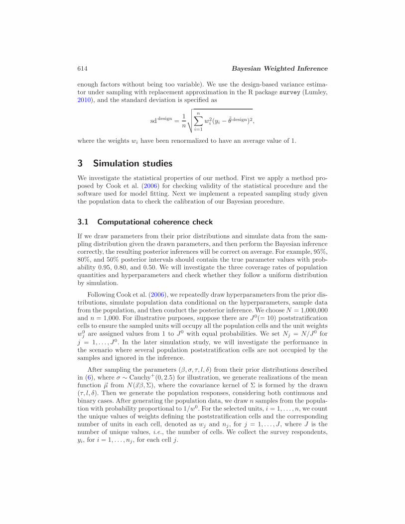
Figure 1: From the computational coherence check for the simulated-data example, cov-erage rates of central 95%, 80%, and 50% posterior intervals for the population quantitiesand hyperparameters in the models for continuous and binary survey responses, cor-respondingly. Each dot represents a coverage rate. The red dots represent the medianvalues.

We use Stan for the posterior computation with Markov chain Monte Carlo (MCMC)algorithm. For the continuous cases, we keep the permuted 3,000 draws from 3 separateMCMC chains after 3,000 warm-up draws. For the binary cases, we keep 6,000 drawsfrom 3 separate MCMC chains after 6,000 warm-up draws. In Stan, each chain takesaround 1 second after compiling. Even though the sample size is large, we need only toinvert a J × J matrix for the likelihood computations for the Gaussian process. Thismatrix inversion is the computational bottleneck in our method.

First, we monitor the convergence of our MCMC algorithm based on one data sam-ple. The convergence measure we use is R based on split chains (Gelman et al., 2013),which when close to 1 demonstrates that chains are well mixed. The collected posteriordraws for our simulations have large enough effective sample sizes neff for the parame-ters, which is calculated conservatively by Stan using both cross-chain and within-chainestimates. The corresponding trace plots also show good mixing behaviors. The posteriormedian values are close to the true values. The posterior summaries for the parame-ters do not change significantly for different initial values of the underlying MCMCalgorithm.

After checking convergence, we implement the process repeatedly 500 times to ex-amine the coverage rates. We compute central 95%, 80%, and 50% intervals using theappropriate quantiles of the posterior simulations.The coverage rates, shown in Figure 1,are close to their expected values for both the continuous and binary survey responses.

616 Bayesian Weighted Inference

We also find the posterior inference for parameters to be robust under different priordistributions, such as inverse-Gamma distribution for τ2, Gamma distribution for l2 ora heavy-tailed prior distribution for β.

4 Simulation ranging from balanced weights to

unbalanced weights

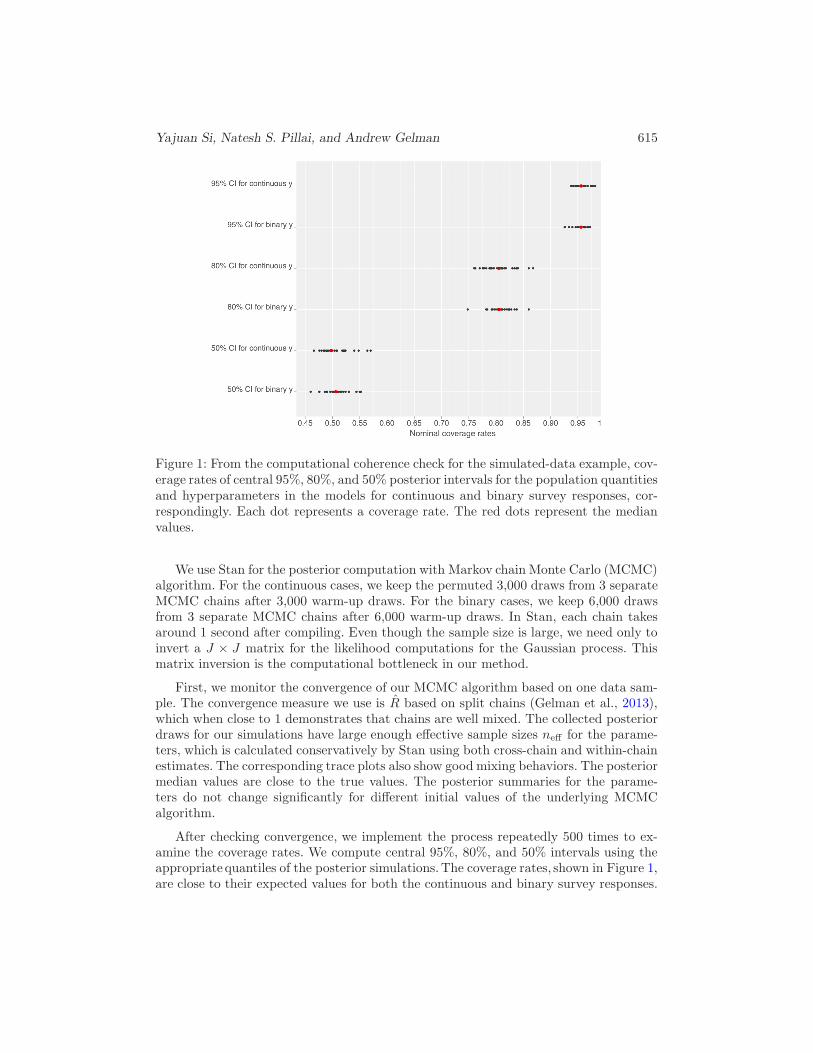
We perform a simulation study comparing performances of the BNFP and the classicalestimate under different sets of weights, ranging from calibration adjustment for onlyone factor to several factors and then getting successively less balanced, with more andmore extreme weights. For constructing the weights in the population, we use externaldata sources to generate the population cell sizes and weights; this allows for cell countsand weights with values close to what is seen in practice. To this end, we borrow a cross-tabulation distribution from the 2013 New York City Longitudinal Survey of Well-being(LSW) conducted by the Columbia Population Research Center. The population in thiscase is adult residents of New York City, defined by the public cross-tabulations from the2011 American Community Survey (ACS) with population size 6,307,213. Four differentsets of weights are constructed via calibration depending on the choice of adjustmentvariables: 1) poverty gap (3 categories), as a poverty measure; 2) poverty gap and race (4categories); 3) poverty gap, race and education (4 categories); and 4) poverty gap, race,education and gender. The cross-tabulations construct J0 = 3, 12, 48 and 96 cell weightsw0, respectively. The unit weights are obtained by the ratio factorsNACS

j /nLSWj ’s, where

NACSj ’s are the ACS cell counts and nLSW

j ’s are the LSW sample cell sizes. We normalizethe population weights to average to 1. The frequency distributions of the constructedweights are shown in Figure 2, which illustrates that the weights become successivelyless balanced. The last two cases have extreme weights, especially for Case 4, of whichthe maximum value is 9.60 and the minimum is 0.19.

Next we simulate the survey variable in the population. For the continuous case, anormal mixture model with different locations is used,

Y ∼ 0.3N(0.5w2, 1) + 0.4N(5 log(w), 1) + 0.3N(5− w, 1).

For the binary outcome,

logitPr(Y = 1) ∼ N(2− 4(log(w) + 0.4)2, 10).

The motivation for the proposed models above is to simulate the population following ageneral distribution with irregular structure, such that we can investigate the flexibilityof our proposed estimator. We perform 100 independent simulations, for each repetitiondrawing a sample from the finite population constructed above with units sampled withprobabilities proportional to 1/w0. We set the sample size as 1000 for the continuousvariable and as 200 for the binary variable.

For each repetition, we also calculate the values of the classical design-based esti-mator with its standard error. Table 1 shows the general comparison: BNFP estimation

Yajuan Si, Natesh S. Pillai, and Andrew Gelman 617

Figure 2: Frequency distributions of constructed unit weights in the population fromfour cases depending on different calibration variables: Case 1 adjusts for poverty gap;Case 2 adjusts for poverty gap and race; Case 3 adjusts for poverty gap, race andeducation; and Case 4 adjusts for poverty gap, race, education and gender. The fourhistograms are on different scales.

performs more efficiently and consistently than the classical estimator in terms of smallerstandard error, smaller actual root mean squared error (RMSE) and better coverage,while both of them are comparable for the reported bias. The improved performancesby BNFP estimation for binary outcomes are more apparent than those with continuousoutcomes mainly due to smaller sample size. The improvement via BNFP estimationis more evident as the weights become less balanced and much noisier. We note thatfor Case 4 with the continuous outcome, the coverages from both approaches are rela-tively low and the bias and RMSE of BNFP are larger than the classical estimator. Wefind that large values of bias and then large RMSE of BNFP estimation correspond tosamples during repetitions when the maximum of the weights is selected but only onesample takes on this value and the simulated y is extremely large, which results in anoutlier. The smoothing property of GPs pulls the cell estimate towards its neighbors.However, the partial pooling offered here is not enough to eliminate the extreme influ-ence of this outlier. This raises the concern on the sensitivity of Bayesian modeling tohighly variable weights and calls for a more informative prior distribution. Another con-cern is that the samples fail to collect all possible weights in the population, especiallyextremely large weights, as an incompleteness of our model, which treats the observedweights as the only possible cells in the population. Consequently, when the outcome is

618 Bayesian Weighted Inference

Data Estimator Avg. S.E. Bias RMSE Coverage95Case 1 BNFP 0.07 −0.00 0.06 97%

classical 0.06 0.01 0.06 97%Case 2 BNFP 0.08 −0.00 0.07 97%

Continuous classical 0.07 0.01 0.07 96%(n = 1000) Case 3 BNFP 0.13 0.03 0.13 95%

classical 0.13 −0.01 0.13 89%Case 4 BNFP 0.17 0.09 0.30 85%

classical 0.21 −0.01 0.27 86%Case 1 BNFP 0.03 −0.01 0.04 93%

classical 0.04 0.00 0.04 92%Case 2 BNFP 0.03 −0.01 0.03 95%

Binary classical 0.04 0.01 0.04 95%(n = 200) Case 3 BNFP 0.03 −0.00 0.03 99%

classical 0.04 0.00 0.04 96%Case 4 BNFP 0.03 0.00 0.02 98%

classical 0.04 −0.00 0.04 94%

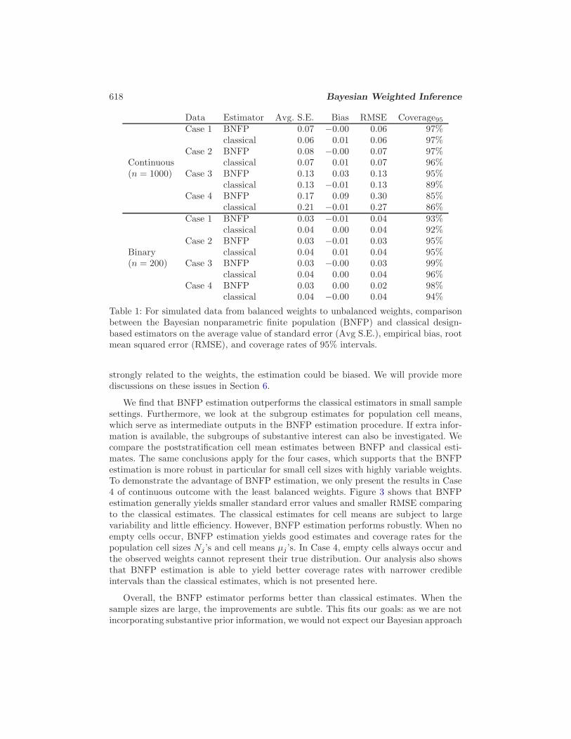
Table 1: For simulated data from balanced weights to unbalanced weights, comparisonbetween the Bayesian nonparametric finite population (BNFP) and classical design-based estimators on the average value of standard error (Avg S.E.), empirical bias, rootmean squared error (RMSE), and coverage rates of 95% intervals.

strongly related to the weights, the estimation could be biased. We will provide morediscussions on these issues in Section 6.

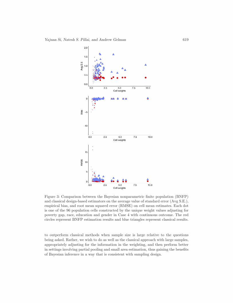
We find that BNFP estimation outperforms the classical estimators in small samplesettings. Furthermore, we look at the subgroup estimates for population cell means,which serve as intermediate outputs in the BNFP estimation procedure. If extra infor-mation is available, the subgroups of substantive interest can also be investigated. Wecompare the poststratification cell mean estimates between BNFP and classical esti-mates. The same conclusions apply for the four cases, which supports that the BNFPestimation is more robust in particular for small cell sizes with highly variable weights.To demonstrate the advantage of BNFP estimation, we only present the results in Case4 of continuous outcome with the least balanced weights. Figure 3 shows that BNFPestimation generally yields smaller standard error values and smaller RMSE comparingto the classical estimates. The classical estimates for cell means are subject to largevariability and little efficiency. However, BNFP estimation performs robustly. When noempty cells occur, BNFP estimation yields good estimates and coverage rates for thepopulation cell sizes Nj’s and cell means µj ’s. In Case 4, empty cells always occur andthe observed weights cannot represent their true distribution. Our analysis also showsthat BNFP estimation is able to yield better coverage rates with narrower credibleintervals than the classical estimates, which is not presented here.

Overall, the BNFP estimator performs better than classical estimates. When thesample sizes are large, the improvements are subtle. This fits our goals: as we are notincorporating substantive prior information, we would not expect our Bayesian approach

Yajuan Si, Natesh S. Pillai, and Andrew Gelman 619

Figure 3: Comparison between the Bayesian nonparametric finite population (BNFP)and classical design-based estimators on the average value of standard error (Avg S.E.),empirical bias, and root mean squared error (RMSE) on cell mean estimates. Each dotis one of the 96 population cells constructed by the unique weight values adjusting forpoverty gap, race, education and gender in Case 4 with continuous outcome. The redcircles represent BNFP estimation results and blue triangles represent classical results.

to outperform classical methods when sample size is large relative to the questions

being asked. Rather, we wish to do as well as the classical approach with large samples,

appropriately adjusting for the information in the weighting, and then perform better

in settings involving partial pooling and small area estimation, thus gaining the benefits

of Bayesian inference in a way that is consistent with sampling design.

620 Bayesian Weighted Inference

5 Application to Fragile Families and Child Wellbeing

Study

The Fragile Families and Child Wellbeing Study (Reichman et al., 2001) follows a co-hort of nearly 5,000 children born in the U.S. between 1998 and 2000 and includes anoversample of nonmarital births. The study addresses the conditions and capabilities ofunmarried parents, especially fathers, and the welfare of their children. The core studyconsists of interviews with both mothers and fathers at the child’s birth and again whenchildren are ages one, three, five, and nine. The sampling design is multistage (sequen-tially sampling cities, hospitals, and births) and complex–involving stratified sampling,cluster sampling, probability-proportional-to-size sampling, and random selection withpredetermined quota. There are two main kinds of unit weights: national weights andcity weights. Applying the national weights (Carlson, 2008) makes the data from the16 randomly selected cities representative of births occurring in large cities in the U.S.between 1998 and 2000. The city weights make the records selected inside each cityrepresentative of births occurring in this city between 1998 and 2000 and adjust forselection bias, nonresponse rates, benchmarking calibration on mother’s marital status,age, ethnicity, and education information at the baseline.

For our example here, we work with the New York City weights and a binary surveyresponse of whether the mother received income from public assistance or welfare orfood stamp services. We perform two analyses, one for the baseline survey and one forthe Year 9 follow-up survey. At baseline, the sample has n = 297 births and J = 161poststratification cells corresponding to the unique values of the weights. Most of thenonempty cells in the sample are occupied by only one or two cases. In Year 9, the samplecontained n = 193 births, corresponding to J = 178 unique values for the weights, witheach cell containing 1 or 2 units. We implement the BNFP procedure using its defaultsettings (as described in Section 2) by Stan, running three parallel MCMC chains with10,000 iterations, which we found more than sufficient for mixing of the chains andfacilitates the posterior predictive checks as follows.

We assess the fit of the model to data using posterior predictive checks (Gelmanet al., 1996). We generate replicated data yrep from their posterior predictive distri-butions given the model and the data and calculate the one sided posterior predictivep-values, Pr(T (yrep) ≥ T (y)|y, φ), where T (y) is the test statistic and φ representsmodel parameters. A p-value close to 0 indicates a lack of fit in the direction of T (y).Here we use the sample total y(j) of responses in cells j as the test statistics T (y),following a general recommendation to check the fit of aspects of a model that are ofapplied interest, and we obtain yrep,l(j) based on posterior samples of parameter φl, for

l = 1, . . . , L. The posterior predictive p-value is computed as 1L

∑Ll=1 I(y

rep,l(j) ≥ y(j)),

for each cell j = 1, . . . , J . At baseline, among the obtained 161 posterior predictivep-values, the minimum is 0.70. In Year 9, the 178 posterior predictive p-values are allabove 0.55. Most p-values are around 0.75, which does not provide significant evidenceagainst the model, indicating the fitting performs well.

At baseline, BNFP estimation yields a posterior mean for the proportion gettingpublic support p of 0.20 with standard error 0.023 and 95% posterior interval (0.16, 0.25).

Yajuan Si, Natesh S. Pillai, and Andrew Gelman 621

Data Parameter Mean Median SD 2.5% 97.5%Baseline p 0.20 0.20 0.02 0.16 0.25

β −0.40 −0.37 0.21 −0.91 −0.07τ 1.74 1.53 0.92 0.69 4.10l 1.75 1.01 17.69 0.30 3.92δ 0.38 0.35 0.23 0.04 0.85

Year 9 p 0.45 0.45 0.03 0.39 0.51β −0.34 −0.26 0.39 −1.36 0.21τ 3.37 2.74 2.42 1.02 9.60l 1.44 1.32 0.70 0.40 3.13δ 0.36 0.35 0.21 0.04 0.78

Table 2: For the Fragile Families Study, Bayesian nonparametric finite-population(BNFP) inferences for model parameters for responses to the public support question.We find greater uncertainty and greater variability for the Year 9 follow-up, comparedto the baseline.

The BNFP estimator is larger than the design-based estimator of 0.16, which has asimilar standard error of 0.024. In Year 9, the BNFP posterior mean for p is 0.45 withstandard error 0.030 and 95% posterior interval (0.39, 0.51). The BNFP estimator islarger than the design-based estimator of 0.32, which has a larger standard error of0.044. Comparing to the baseline survey when the child was born, the estimate of theproportion of mothers receiving public support services increases when the child wasYear 9. This is expected since child care in fragile families needs more social support asthe child grows up and some biological fathers become much less involved.

The posterior summaries for the hyperparameters are shown in Table 2. The pos-terior mean of the scale τ is larger in the follow-up sample than in the baseline, whichillustrates larger variability for the cell mean probabilities. As seen from Figure 4, thepoststratification cell mean probabilities depend on the unit weights in cells in an irreg-ular structure. Because the Nj ’s are not normalized, we look at the poststratificationcell size proportions Npj(= Nj/

∑

Nj). Since most sample cell sizes are 1, we see ageneral increasing pattern between the poststratification cell size proportions and theunit weights in cell j, for j = 1, . . . , J . The uncertainty is large due to the small samplecell sizes. These conclusions hold for both the baseline and the follow-up survey. In thefollow-up survey, the correlation between the cell mean probabilities is stronger andmore variable compared to those in the baseline survey.

6 Discussion

We have demonstrated a nonparametric Bayesian estimation for population inferencefor the problem in which inverse-probability sampling weights on the observed unitsrepresent all the information that is known about the design. Our approach proceeds byestimating the weights for the nonsampled units in the population and simultaneouslymodeling the survey outcome given the weights as predictors using a robust Gaussianprocess regression model. This novel procedure captures uncertainty in the sampling

622 Bayesian Weighted Inference

Figure 4: Estimated Fragile Families survey population poststratification cell mean prob-abilities θj and cell size proportions Npj for unit weights in different cells. Red dots arethe posterior mean estimates and the black vertical lines are the 95% posterior credibleintervals. Dot sizes are proportional to sample cell sizes nj ; the top two plots are forthe baseline survey and the bottom two are for the follow-up survey.

as well as in the unobserved outcomes. We implement the model in Stan, a flexibleBayesian inference environment that can allow the model to be easily expanded toinclude additional predictors and levels of modeling, as well as alternative link functionsand error distributions. In simulation studies, our fully Bayesian approach performs wellcompared to classical design-based inference. Partial pooling across small cells allowsthe Bayesian estimator to be more efficient in terms of smaller variance, smaller RMSE,and better coverage rates.

Our problem framework is clean in the sense of using only externally-supplied sur-vey weights, thus representing the start of an open-ended framework for model-basedinference based on the same assumptions as the fundamental classical model of inverse-probability weighting. There are many interesting avenues for development. When thevariables used to construct the weights are themselves available, they can be includedin the model (Gelman, 2007). A natural next step is to model interactions among thesevariables. Multilevel regression and poststratification have achieved success for subpop-ulation estimations at much finer levels. More design information or covariates can beincorporated. Another direction to explore is to extend our framework when we have

Yajuan Si, Natesh S. Pillai, and Andrew Gelman 623

only partial census information, for example, certain margins and interactions but notthe full cross-tabulations. Our approach can be used to make inference on the unknowncensus information, such as the population cell sizes Nj’s. This also facilitates smallarea estimation under a hierarchical modeling framework.

Two concerns remain about our method. First, the inferential procedure assumesthat all unique values of the weights have been observed. If it is deemed likely thatthere are some large weights in the population that have not occurred in the sample,this will need to be accounted for in the model, either as a distribution for unobservedweight values, or by directly modeling the factors that go into the construction of theweights. Under an appropriate hierarchical modeling framework, we can partially poolthe data and make inference on the empty cells, borrowing information from observednonempty cells. Second, in difficult problems (those with a few observations with verylarge weights), our inference will necessarily be sensitive to the smoothing done at thehigh end, in particular the parametric forms of the model for the Nj ’s and the regressionof y|w. This is the Bayesian counterpart to the instability of classical inferences whenweights are highly variable. In practical settings in which there are a few observationswith very large weights, these typically arise by multiplying several moderately-largefactors. It should be possible to regain stability of estimation by directly modeling thefactors that go into the weights with main effects and partially pooling the interactions;such a procedure should outperform simple inverse-probability weighting by virtue ofusing additional information not present in the survey weights alone. But that is asubject for future research. In the present paper we have presented a full Bayesiannonparametric inference using only the externally-supplied survey weights, with theunderstanding that inference can be improved by including additional information.

References

Carlson, B. L. (2008). “Fragile Families and Child Wellbeing Study: Methodology forconstructing mother, father, and couple weights for core telephone surveys waves 1-4.”Technical report, Mathematica Policy Research. 620

CBS News/New York Times (1988). Monthly Poll, July 1988 . Inter-university Consor-tium for Political and Social Research, University of Michigan. 605

Chen, Q., Elliott, M. R., and Little, R. J. (2010). “Bayesian penalized spline model-based inference for finite population proportion in unequal probability sampling.”Survey Methodology, 36(1): 23–34. 609

Cook, S., Gelman, A., and Rubin, D. B. (2006). “Validation of software for Bayesianmodels using posterior quantiles.” Journal of Computational and Graphical Statistics ,15: 675–692. 614

Elliott, M. R. (2007). “Bayesian weight trimming for generalized linear regression mod-els.” Journal of Official Statistics , 33(1): 23–34. 609

Elliott, M. R. and Little, R. J. (2000). “Model-based alternatives to trimming surveyweights.” Journal of Official Statistics , 16(3): 191–209. 609

624 Bayesian Weighted Inference

Gelman, A. (2006). “Prior distributions for variance parameters in hierarchical models.”Bayesian Analysis , 3: 515–533. 613

— (2007). “Struggles with survey weighting and regression modeling (with discussion).”Statistical Science, 22(2): 153–164. 605, 622

Gelman, A. and Carlin, J. B. (2001). “Poststratification and weighting adjustments.”In Groves, R., Dillman, D., Eltinge, J., and Little, R. (eds.), Survey Nonresponse.607

Gelman, A., Carlin, J. B., Stern, H. S., Dunson, D. B., Vehtari, A., and Rubin, D. B.(2013). Bayesian Data Analysis . CRC Press, London, 3rd edition. 615

Gelman, A., Jakulin, A., Pittau, M. G., and Su, Y.-S. (2008). “A weakly informativedefault prior distribution for logistic and other regression models.” Annals of Applied

Statistics , 2(4): 1360–1383. 612

Gelman, A. and Little, T. C. (1997). “Poststratifcation into many cateogiries usinghierarchical logistic regression.” Survey Methodology, 23: 127–135. 607

Gelman, A., Meng, X.-L., and Stern, H. S. (1996). “Posterior predictive assessment ofmodel fitness via realized discrepancies.” Statistica Sinica, 6: 733–807. 620

Ghitza, Y. and Gelman, A. (2013). “Deep interactions with MRP: Election turnoutand voting patterns among small electoral subgroups.” American Journal of Political

Science, 57: 762–776. 606

Hajek, J. (1971). “Comment on “An Essay on the logical foundations of survey sam-pling” by D. Basu.” In Godambe, V. P. and Sprott, D. A. (eds.), The Foundations

of Survey Sampling, 236. Holt, Rinehart and Winston. 607

Hoffman, M. D. and Gelman, A. (2014). “The No-U-Turn sampler: Adaptively settingpath lengths in Hamiltonian Monte Carlo.” Journal of Machine Learning Research,15: 1351–1381. 609

Horvitz, D. G. and Thompson, D. J. (1952). “A generalization of sampling withoutreplacement from a finite university.” Journal of the American Statistical Association,47(260): 663–685. 607

Lax, J. and Phillips, J. (2009a). “Gay rights in the states: Public opinion and policyresponsiveness.” American Political Science Review , 103: 367–386. 606

— (2009b). “How should we estimate public opinion in the states?” American Journal

of Political Science, 53: 107–121. 606

Little, R. J. (1983). “Comment on “An evaluation of model-dependent and probability-sampling inferences in sample surveys” by M. H. Hansen, W. G. Madow and B. J.Tepping.” Journal of the American Statistical Association, 78: 797–799. 606

— (1991). “Inference with survey weights.” Journal of Official Statistics , 7: 405–424.607

— (1993). “Post-stratification: A modeler’s perspective.” Journal of the American

Statistical Association, 88: 1001–1012. 607

Yajuan Si, Natesh S. Pillai, and Andrew Gelman 625

Lumley, T. (2010). Complex Surveys: A Guide to Analysis Using R. Wiley, New York.614

Oleson, J. J., He, C., Sun, D., and Sheriff, S. (2007). “Bayesian estimation in small areaswhen the sampling design strata differ from the study domains.” Survey Methodology,33: 173–185. 608

Polson, N. G. and Scott, J. G. (2012). “On the half-Cauchy prior for a global scaleparameter.” Bayesian Analysis , 7(2): 1–16. 613

Rasmussen, C. E. and Williams, C. K. I. (2006). Gaussian Processes for Machine

Learning. MIT Press, Cambridge, Mass. 611

Reichman, N. E., Teitler, J. O., Garfinkel, I., and McLanahan, S. S. (2001). “FragileFamilies: Sample and design.” Children and Youth Services Review , 23(4/5): 303–326.620

Rubin, D. B. (1983). “Comment on “An evaluation of model-dependent and probability-sampling inferences in sample surveys” by M. H. Hansen, W. G. Madow and B. J.Tepping.” Journal of the American Statistical Association, 78: 803–805. 606

Stan Development Team (2014a). “Stan: A C++ Library for Probability and Sampling,version 2.2.” http://mc-stan.org/. 609

— (2014b). Stan Modeling Language User’s Guide and Reference Manual, version 2.2 .http://mc-stan.org/. 609

van der Vaart, A. W. and van Zanten, J. H. (2008). “Rates of contraction of posteriordistributions based on Gaussian process priors.” Annals of Statistics , 36(3): 1435–1463. 611

Zangeneh, S. Z. and Little, R. J. (2012). “Bayesian inference for the finite populationtotal from a heteroscedastic probability proportional to size sample.” Proceedings of

the Joint Statistical Meetings, Section on Survey Methodology. 608, 609

Zheng, H. and Little, R. J. (2003). “Penalized spline model-based estimation of thefinite populations total from probability-proportional-to-size samples.” Journal of

Official Statistics , 19(2): 99–107. 609, 611

Acknowledgments

We thank the National Science Foundation, the Institute of Education Sciences, the Office of

Naval Research, the Robin Hood Foundation, and the Fragile Families Study project for partial

support of this work.