Bayesian Nonparametric Autoregressive Modelsvia Latent Variable Representation

Maria De Iorio

Yale-NUS CollegeDept of Statistical Science, University College London

Collaborators: Lifeng Ye (UCL, London, UK)Alessandra Guglielmi (Polimi, Milano, Italy)

Stefano Favaro (Universita degli Studi di Torino, Italy)

29th August 2018Bayesian Computations for High-Dimensional Statistical Models

Motivation

T=1 T=2 T=3

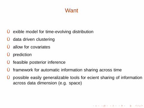
Want

Ü flexible model for time-evolving distribution

Ü data driven clustering

Ü allow for covariates

Ü prediction

Ü feasible posterior inference

Ü framework for automatic information sharing across time

Ü possible easily generalizable tools for efficient sharing of informationacross data dimension (e.g. space)

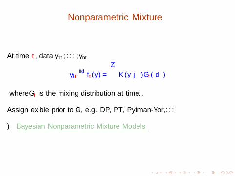
Nonparametric Mixture

At time t, data y1t , . . . , ynt

yitiid∼ ft(y) =

∫K (y | θ)Gt( dθ)

where Gt is the mixing distribution at time t.

Assign flexible prior to G , e.g. DP, PT, Pytman-Yor, . . .

⇒ Bayesian Nonparametric Mixture Models

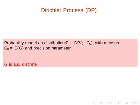
Dirichlet Process (DP)

Probability model on distributions G ∼ DP(α,G0), with measureG0 = E(G ) and precision parameter α.

G is a.s. discrete

Sethuraman’s stick breaking representation

G =∞∑h=1

whδθh

ξh ∼ Beta(1, α)

wh = ξh

h−1∏i=1

(1− ξi ), scaled Beta distribution

θhiid∼ G0, h = 1, 2, . . .

where δ(x) denotes a point mass at x , ψh are weights of point masses atlocations θh.

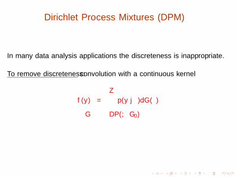
Dirichlet Process Mixtures (DPM)

In many data analysis applications the discreteness is inappropriate.

To remove discreteness: convolution with a continuous kernel

f (y) =

∫p(y | θ)dG (θ)

G ∼ DP(α,G0)

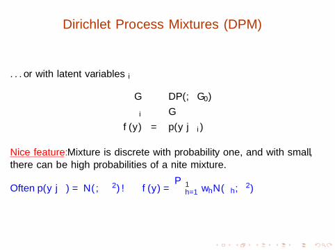
Dirichlet Process Mixtures (DPM)

. . . or with latent variables θi

G ∼ DP(α,G0)

θi ∼ G

f (y) = p(y | θi )

Nice feature: Mixture is discrete with probability one, and with small α,there can be high probabilities of a finite mixture.

Often p(y | θ) = N(β, σ2) −→ f (y) =∑∞

h=1 whN(βh, σ2)

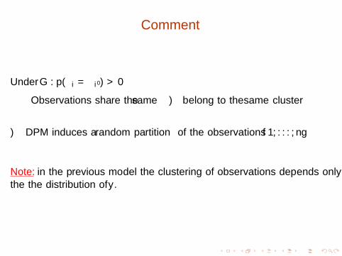
Comment

Under G : p(θi = θi ′) > 0

• Observations share the same θ ⇒ belong to the same cluster

⇒ DPM induces a random partition of the observations {1, . . . , n}

Note: in the previous model the clustering of observations depends only onthe the distribution of y .

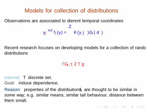
Models for collection of distributions

Observations are associated to different temporal coordinates

ytind∼ ft(y) =

∫K (y | θ)Gt( dθ)

Recent research focuses on developing models for a collection of randomdistributions

{Gt ; t ∈ T }

Interest: T discrete set.Goal: induce dependence.

Reason: properties of the distributions ft are thought to be similar insome way; e.g. similar means, similar tail behaviour, distance betweenthem small.

Dependent Dirichlet Process

If G ∼ DP(G0, α), then using the constructive definition of the DP(Sethuraman 1994)

Gt =∞∑k=1

wtkδθtk

where (θtk)∞k=1 are iid from some G0(θ) and (wtk) is a stick breakingprocess

wtk = ztk∏j<k

(1− ztj)

ztj ∼ Beta(1, αt)

Dependence has been introduced mostly in regression context,conditioning on level of covariates x .

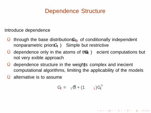
Dependence Structure

Introduce dependence

Ü through the base distributions G0t of conditionally independentnonparametric priors Gt ⇒ Simple but restrictive

Ü dependence only in the atoms of the Gt ⇒ efficient computations butnot very flexible approach

Ü dependence structure in the weights ⇒ complex and inefficientcomputational algorithms, limiting the applicability of the models

Ü alternative is to assume

Gt = πtG + (1− πt)G ?t

Dependence through Weights

• flexible strategy

• random prob measures share the same atoms

• under certain conditions we can approximate any density with anyatoms

• varying the weights can provide prob measures very close (similarweights) or far apart

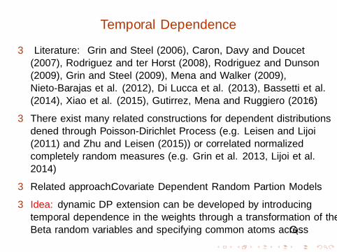
Temporal Dependence

3 Literature: Griffin and Steel (2006), Caron, Davy and Doucet(2007), Rodriguez and ter Horst (2008), Rodriguez and Dunson(2009), Griffin and Steel (2009), Mena and Walker (2009),Nieto-Barajas et al. (2012), Di Lucca et al. (2013), Bassetti et al.(2014), Xiao et al. (2015), Gutirrez, Mena and Ruggiero (2016) . . .

3 There exist many related constructions for dependent distributionsdefined through Poisson-Dirichlet Process (e.g. Leisen and Lijoi(2011) and Zhu and Leisen (2015)) or correlated normalizedcompletely random measures (e.g. Griffin et al. 2013, Lijoi et al.2014)

3 Related approach: Covariate Dependent Random Partion Models

3 Idea: dynamic DP extension can be developed by introducingtemporal dependence in the weights through a transformation of theBeta random variables and specifying common atoms across Gt .

Related Approaches

Gt =∞∑k=1

wtkδθk , wtk = ξtk

k−1∏i=1

(1− ξti ), ξtk ∼ Beta(1, α)

7 BAR Stick–Breaking Process (Taddy 2010): defines evolutionequation for wt :

ξt = (utvt)ξt−1 + (1− ut) ∼ Beta(1, α)

ut ∼ Beta(α, 1− ρ), vt ∼ Beta(ρ, 1− ρ)

0 < ρ < 1, ut ⊥⊥ vt

7 DP marginal, corr(ξt , ξt−k) = [ρα/(1 + α− ρ)]k > 0

7 Prior simulations show that number of clusters and number ofsingletons at time t = 1 is different from other times.

7 Very different clustering can corresponds to relatively similarpredictive distributions.

7 Latent Gaussian time-series (DeYoreo and Kottas 2018):

ξt = exp

{−ζ2 + η2t

2α

}∼ Beta(α, 1)

ζ ∼ N(0, 1)

ηt | ηt−1, φ ∼ N(φηt−1, 1− φ2), |φ| < 1

wt1 = 1− ξt1, wtk = (1− ξtk)k−1∏i=1

ξti

ηt AR(1) process.

7 α ≥ 1 implies a 0.5 lower bound on corr(ξt , ξt−k). As a result, sameweights (For example, the first weight at time 1 and first weight attime 2) always have correlation above 0.5.

7 η (AR component) is squared so that the correlation betweendifferent times is positive.

7 These problems can be overcome by assuming time-varying locations.

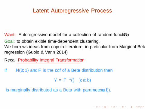
Latent Autoregressive Process

Want: Autoregressive model for a collection of random function Gt .

Goal: to obtain flexible time-dependent clustering.We borrows ideas from copula literature, in particular from Marginal Betaregression (Guolo & Varin 2014)

Recall Probability Integral Transformation:

If ε ∼ N(0, 1) and F is the cdf of a Beta distribution then

Y = F−1(Φ(ε); a, b)

is marginally distributed as a Beta with parameters (a, b).

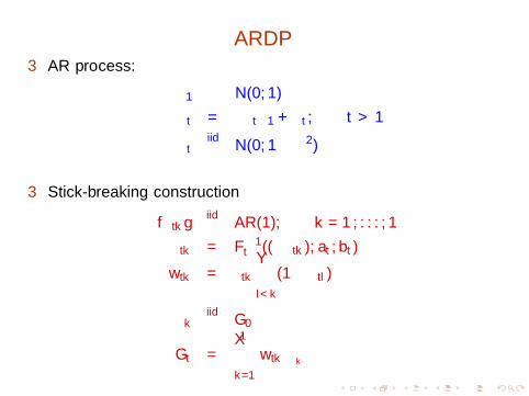
ARDP3 AR process:

ε1 ∼ N(0, 1)

εt = ψεt−1 + ηt , t > 1

ηtiid∼ N(0, 1− ψ2)

3 Stick-breaking construction

{εtk}iid∼ AR(1), k = 1, . . . ,∞

ξtk = F−1t (Φ(εtk); at , bt)

wtk = ξtk∏l<k

(1− ξtl)

θkiid∼ G0

Gt =∞∑k=1

wtkδθk

Comments

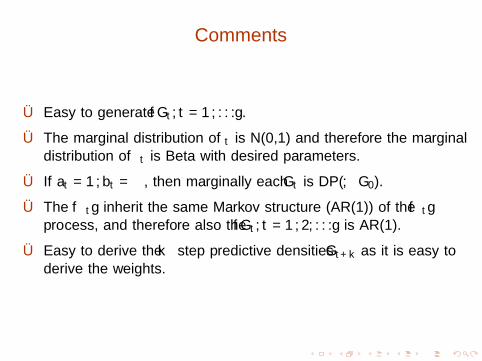
Ü Easy to generate {Gt , t = 1, . . .}.

Ü The marginal distribution of εt is N(0,1) and therefore the marginaldistribution of ξt is Beta with desired parameters.

Ü If at = 1, bt = α, then marginally each Gt is DP(α,G0).

Ü The {ξt} inherit the same Markov structure (AR(1)) of the {εt}process, and therefore also the {Gt , t = 1, 2, . . .} is AR(1).

Ü Easy to derive the k−step predictive densities Gt+k as it is easy toderive the weights.

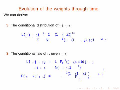
Evolution of the weights through timeWe can derive:

3 The conditional distribution of ξt | ξt−1:

L(ξt | ξt−1)d= 1− (1− Φ(Z ))1/α

Z ∼ N(ψΦ−1 (1− (1− ξt−1)α) , 1− ψ2

).

3 The conditional law of ξt , given εt−1:

L{ξt | εt−1} = L{F−1t (Φ(εt); a, b) | εt−1

}εt | εt−1 ∼ N(ψεt−1, 1− ψ2)

P(ξt ≤ x | εt−1) = Φ

(Φ−1(1− (1− x)α)− ψεt−1√

1− ψ2

)

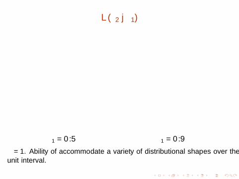
L(ξ2 | ξ1)

0.0 0.2 0.4 0.6 0.8 1.0

0.0

0.5

1.0

1.5

2.0

2.5

psi=0psi=0.9psi=−0.5

0.0 0.2 0.4 0.6 0.8 1.0

01

23

45

psi=0psi=0.9psi=−0.5

ξ1 = 0.5 ξ1 = 0.9

α = 1. Ability of accommodate a variety of distributional shapes over theunit interval.

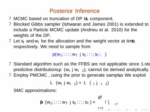
Posterior Inference7 MCMC based on truncation of DP to L component.7 Blocked Gibbs sampler (Ishwaran and James 2001) is extended to

include a Particle MCMC update (Andrieu et al. 2010) for theweights of the DP.

7 Let st and wt be the allocation and the weight vector at time t,respectively. We need to sample from

p(w1, . . . ,wT | s1 . . . , sT , ψ)

7 Standard algorithm such as the FFBS are not applicable since 1-steppredictive distributions, pψ(wt | wt−1), cannot be derived analytically.

7 Employ PMCMC , using the prior to generate samples εt . We exploit

Lψ(wt | wt−1) = Lψ(εt | εt−1)

SMC approximations:

pψ(w1, . . . ,wT | s1 . . . , sT ) =R∑

r=1

ωrT δε1:T

Simulations

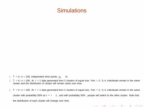
– T = 4, n = 100, independent time points, yit ∼ N.

– T = 4, n = 100. At t = 1 data generated from 2 clusters of equal size. For t = 2, 3, 4, individuals remain in the samecluster and the distribution of cluster will remain same over time.

– T = 4, n = 100. At t = 1 data generated from 2 clusters of equal size. For t = 2, 3, 4, individuals remain in the same

cluster with probability 50% as t = i − 1 , and with probability 50% , people will switch to the other cluster. Note that

the distribution of each cluster will change over time.

Disease Mapping

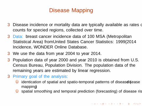
3 Disease incidence or mortality data are typically available as rates orcounts for specified regions, collected over time.

3 Data: breast cancer incidence data of 100 MSA (MetropolitanStatistical Area) from United States Cancer Statistics: 1999–2014Incidence, WONDER Online Database.

3 We use the data from year 2004 to year 2014.

3 Population data of year 2000 and year 2010 is obtained from U.S.Census Bureau, Population Division. The population data of theremaining years are estimated by linear regression.

3 Primary goal of the analysis:Ü identification of spatial and spatio-temporal patterns of disease (disease

mapping)Ü spatial smoothing and temporal prediction (forecasting) of disease risk.

Space-Time Clustering

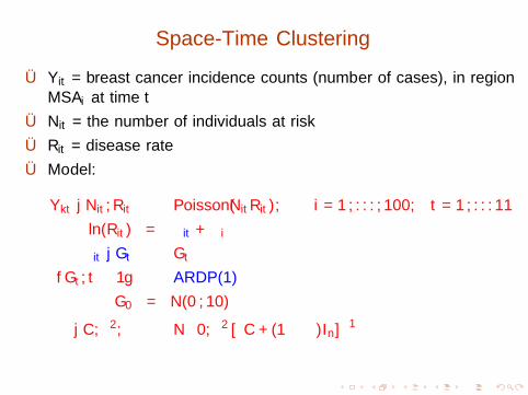
Ü Yit = breast cancer incidence counts (number of cases), in regionMSAi at time t

Ü Nit = the number of individuals at risk

Ü Rit = disease rate

Ü Model:

Ykt | Nit ,Rit ∼ Poisson(NitRit), i = 1, . . . , 100; t = 1, . . . 11

ln(Rit) = µit + φi

µit | Gt ∼ Gt

{Gt , t ≥ 1} ∼ ARDP(1)

G0 = N(0, 10)

φ | C, τ2, ρ ∼ N(

0, τ2 [ρC + (1− ρ)In]−1)

Spatial Component

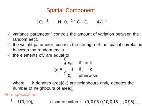
φ | C, τ2, ρ ∼ N(

0, τ2 [ρC + (1− ρ)In]−1)

– variance parameter τ2 controls the amount of variation between therandom effect.

– the weight parameter ρ controls the strength of the spatial correlationbetween the random effects

– the elements of C are equal to

cjk =

nk , if j = k

−1, if j ∼ k

0, otherwise.

where j ∼ k denotes area (j , k) are neighbours and nk denotes thenumber of neighbours of area (k).

Prior specification:

τ2 ∼ U(0, 10), ρ ∼ discrete uniform(0, 0.05, 0.10, 0.15, ..., 0.95)

Posterior Inference on Clustering

Co-Clustering Probability

Posterior Inference on Correlations

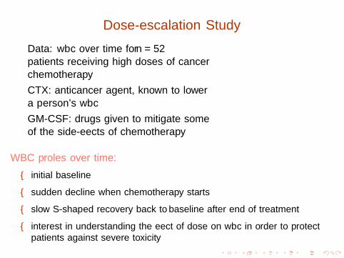
Dose-escalation Study

• Data: wbc over time for n = 52patients receiving high doses of cancerchemotherapy

• CTX: anticancer agent, known to lowera person’s wbc

• GM-CSF: drugs given to mitigate someof the side-effects of chemotherapy

WBC profiles over time:

– initial baseline

– sudden decline when chemotherapy starts

– slow S-shaped recovery back to ≈ baseline after end of treatment

– interest in understanding the effect of dose on wbc in order to protectpatients against severe toxicity

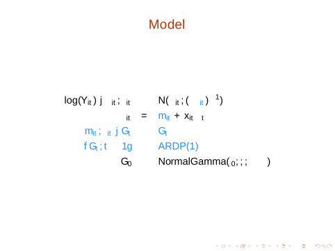
Model

log(Yit) | µit , τit ∼ N(µit , (λτit)−1)

µit = mit + xitβt

mit , τit | Gt ∼ Gt

{Gt , t ≥ 1} ∼ ARDP(1)

G0 ∼ NormalGamma(µ0, λ, α, γ)

Posterior Inference on ψ

Posterior Inference on Clustering

Posterior Density Estimation

Conclusions

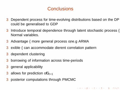
3 Dependent process for time-evolving distributions based on the DP —could be generalised to GDP

3 Introduce temporal dependence through latent stochastic process –Normal variables.

3 Advantage – more general process on ε, e.g ARMA

3 flexible – can accommodate different correlation pattern

3 dependent clustering

3 borrowing of information across time-periods

3 general applicability

3 allows for prediction of Gt+1

3 posterior computations through PMCMC