Bayesian Non-parametric Generation of Fully Synthetic...

Bayesian Non-parametric Generation of Fully Synthetic Multivariate

Categorical Data in the Presence of Structural Zeros

Daniel Manrique-Vallier

Department of Statistics, Indiana University, Bloomington, IN 47408, USA

E-mail: [email protected]†

Jingchen Hu

Department of Mathematics and Statistics, Vassar College, Poughkeepsie, NY 12604, USA

E-mail: [email protected]

Summary. Statistical agencies are increasingly adopting synthetic data methods for disseminating micro-

data without compromising the privacy of respondents. Crucial to the implementation of these approaches

are flexible models, able of capturing the nuances of the multivariate structure present in the original data.

In the case of multivariate categorical data, preserving this multivariate structure also often involves satisfy-

ing constrains in the form of combinations of responses that cannot logically be present in any dataset—like

married toddlers or pregnant men—also known as structural zeros. Ignoring structural zeros can result in

both logically inconsistent synthetic data and biased estimates. Here we propose the use of a Bayesian

non-parametric method for generating discrete multivariate synthetic data subject to structural zeros. This

method can preserve complex multivariate relationships between variables; can be applied to high dimen-

sional datasets with massive collections of structural zeros; requires minimal tuning from the user; and is

computationally efficient. We demonstrate our approach by synthesizing an extract of 17 variables from

the 2000 U.S. Census. Our method produces synthetic samples with high analytic utility and low disclosure

risk.

Keywords: Bayesian Nonparametric, Dirichlet Process, Contingency Tables, Multiple Imputation,

MCMC, Disclosure Risk

†Address for correspondence: [email protected]

2 Manrique-Vallier, D. and Hu, J.

1. Introduction

The use of synthetic data (Rubin, 1993) is an attractive option for statistical agencies and other organi-

zations that wish to share individual-level data with third parties, but at the same wish to protect the

identities and sensitive attributes of respondents. The idea is simple. The data custodian (henceforth

“the agency”) uses the sensitive data to fit a statistical model, and releases samples from its predictive

distribution instead of the original data. Secondary analysts can then perform analyses on the synthetic

data without having access to the original data. In order to account for the uncertainty associated with

the sampling and estimation procedures, the agency can release a set of M approximately independent

samples from the predictive distribution, which then analysts can combine using the rules developed

specifically for synthetic data by Raghunathan et al. (2003).

The utility of synthetic data schemes depends heavily on the quality of the models used to generate

the data: analysts will be unable to detect features that the synthesis model did not adequately capture

in the first place. In the case of multivariate data, synthesis models have to be prepared to preserve

complex—and often unexplored—relationships between variables. A popular synthesis technique is the

sequential modeling or full conditional specification (FCS) approach (Van Buuren and Oudshoorn, 1999;

Van Buuren et al., 2006). Here the agency fits regression models to each of the variables conditional

on the rest, and then use them for sampling each variable, one at a time. Greater flexibility can be

achieved by using non-parametric regression models such as CART and random forests (Reiter, 2005;

Caiola and Reiter, 2010). This approach has the advantage of simplicity, replacing the problem of

specifying a complex multivariate distribution with the simpler problem of specifying several univariate

conditional models. However, as has been noted (e.g. Raghunathan et al., 2001; Vermunt et al., 2008;

White et al., 2011), this procedure lacks guarantees that the resulting set of regression models will

correspond to any well-defined joint distribution. Moreover, when dealing with certain configurations

of categorical data, it lacks the ability of sampling from the whole support of the distribution. We

comment on this specific problem in the discussion.

A second approach to synthetic data generation is the use of joint probability models. This approach

avoids most of the pitfalls of sequential conditional modeling, but has the drawbacks of estimation

complexity, and the need of finding and selecting models with good predictive performance. In the

case of discrete data, most early proposals using joint modeling have focused on simple models, like the

Synthetic Data with Structural Zeros 3

discretized multivariate normal (Matthews et al., 2010). More recently, Hu et al. (2014) proposed the

use of a Bayesian non-parametric version of the Latent Class (NPLCM) model proposed by Dunson

and Xing (2009) to synthesize multivariate categorical data. They showed that this model enjoys a

good predictive performance, scalability, and low disclosure risk.

An important issue that Hu et al. (2014) did not address was the case of structural restrictions

in the form of responses that are known to be impossible a priori, known as structural zeros (Bishop

et al., 1975)—for example, it is impossible for a toddler to be a widower. An obvious problem with

not explicitly accounting for structural zeros is the risk of assigning positive probability to impossible

combinations, and thus of generating and disseminating synthetic data with inconsistent responses (like

widower toddlers). Such synthetic data could cause confusion in analysts, and ultimately lead to the

public’s losing of confidence in the agency’s work. Additionally, as Manrique-Vallier and Reiter (2014)

noted, failing to account for structural zeros can lead to biased estimates.

In this article we propose and evaluate the use of an extension of the NPLCM, originally introduced

by Manrique-Vallier and Reiter (2014), for the task of synthesizing discrete multivariate data subject

to structural zeros. This extension, called the Truncated NPLCM (TNPLCM), retains most of the

advantages described by Hu et al. (2014) while adding the ability of handling complex patterns of

structural zeros. We present a considerably improved computational method to fit the TNPLCM

(Sections 2.2 and 2.3), and extend it to the task of generating fully synthetic data (Section 2.4). We

illustrate the use of our approach by synthesizing an extract of 17 categorical variables from the U.S.

2000 census, which results in a contingency table of about 55 × 109 cells from which about 52 × 109

correspond to structural zeros. Through a demanding battery of tests we show that the TNPLCM

generates high-utility synthetic data (Section 3.1) with low-disclosure risk (Section 3.2).

2. Nonparametric Latent Class Models for Categorical Data Synthesis

Suppose that the agency has collected a sample of n individual confidential records, each detailing

J attributes with finitely many possible values. Let X = (x1, ...,xn) be the original sample, xi =

(xi1,, ..., xiJ) each record, and Cj = 1, ..., Lj the set of possible values of xij . Thus for any individual

i ∈ 1, ..., n we have that in principle xi ∈ C =∏Jj=1 Cj . Following standard terminology we call each

of the elements of C a cell. Let S ⊂ C be a set for which it is known a priori that Pr(x ∈ S) = 0. We


call the cells in S structural zeros (Bishop et al., 1975). Our objective is to use X to generate M fully

synthetic datasets Y = (Y1, ..,YM ), with support in C \ S, which can be safely disseminated, and that

lead to inferences close to those which would be obtained from X itself.

2.1. Nonparametric Latent class models

Hu et al. (2014) proposed the use of the nonparametric latent class model (NPLCM) as a data-

synthesizer for high-dimensional discrete categorical data without structural zeros. Here we describe

it in preparation for discussing the issues involved in considering the structural zeros. The NPLCM is

a Dirichlet process mixture of product-multinomial distributions, originally proposed by Dunson and

Xing (2009) as a general-purpose tool for modeling complex contingency tables. As Dunson and Xing

(2009) show, the NPLCM has full support in C. Thus it is consistent for estimating cell probabilities in

any contingency table. Additional practical advantages include its computational tractability and scal-

ability, its tolerance to severely sparse contingency tables, and its minimal need for tuning by the user

(see e.g. Si and Reiter, 2013; Manrique-Vallier and Reiter, 2014; Manrique-Vallier, 2016, for example

applications in different domains).

The construction of the NPLCM model in Dunson and Xing (2009) is similar to the classic La-

tent Class model (Goodman, 1974). We assume that the population can be partitioned into a finite

number of homogeneous classes, and that within each of these classes item responses can be considered

independent—conditional independence given class membership. This can be expressed as the following

generative model

xijind∼ Discrete(1, ..., Lj, (λjzi [1], ..., λjzi [Lj ])), for i = 1, .., n, j = 1, ..., J (1)

zi ∼ Discrete(1, ...,K, (π1, ..., πK)), for i = 1, ..., n , (2)

where the class assignment labels, zi, and their probabilities, πi are unknown. Dunson and Xing (2009)

construct the NPLCM by considering an infinite number of classes, and assigning a stick-breaking prior

(Sethuraman, 1994) for their (infinite dimensional) probability vector. The version of the NPLCM

proposed by Hu et al. (2014) for data synthesis is a computationally convenient finite-dimensional


approximation to this model. We describe it by completing the LCM model in (1)-(2) with

π = (π1, ..., πK) ∼ SBK(α) (3)

λjk[·]iid∼ Dirichlet(1Lj

), for j = 1, ..., J and k = 1, ...,K (4)

α ∼ Gamma(a, b) (5)

where SBK(α) is the finite dimensional stick-breaking process (Ishwaran and James, 2001): for k =

1, ...,K make πk = Vk∏h<K(1 − Vh), where VK = 1 and Vk ∼ Beta(1, α) for k < K. Here SBK(α)

replaces the infinite-dimensional stick breaking process from Dunson and Xing (2009); see Si and Reiter

(2013) and Manrique-Vallier and Reiter (2014) for guidance about choosing K. We also follow Dunson

and Xing (2009) in setting a = b = 0.25 as a weak prior that favors a data-dominated inference.

2.2. NPLCM with Structural Zeros

Manrique-Vallier and Reiter (2014) developed an extension to the NPLCM, henceforth denoted TNPLCM

(Truncated NPLCM), which allows to enforce the restriction Pr(x ∈ S) = 0 for some known set of struc-

tural zeros S ⊂ C. Their computational method relies on a sample augmentation technique whereby

we assume the existence of an unobserved sample X 0 = (x1, ...,xn0) of unknown size n0 = N − n,

generated from the unrestricted NPLCM, but which contains only records whose values fall into S.

Manrique-Vallier and Reiter (2014) showed that setting the improper prior distribution P (N) ∝ 1/N

and estimating X 0 and their corresponding latent variables Z0 = (z1, ..., zn0) simultaneously with the

rest of the parameters involved in the model in (1)-(2), results in the same marginal posterior dis-

tribution of (λ,π) corresponding to the TNPLCM. We note that under this scheme, computing the

predictive distribution of the TNPLCM for a given set of parameters (λ,π) requires truncating and

re-normalizing the pmf so that fTNPLCM (x|π,λ, S) ∝ I(x /∈ S)∑K

k=1 πk∏Jj=1 λjk[xj ].

Manrique-Vallier and Reiter (2014) also noted that significant computational gains can be realized

whenever s can be expressed as the union of a relatively small (with respect to the size of s) collection of

disjoint table slices. A table slice is the collection of cells that result from fixing some of the j response

components, while letting the rest take any possible value—for example the set x = (x1, ..., x6) ∈ C :

x1 = 1, x3 = 4. Real situations in which this is possible are frequent; it is common that structural


zeros arise from specific combinations of levels of a few (often just two) variables at a time. When the

resulting collection of slices is not disjoint, we need to transform them into a disjoint collection using

the specialized algorithm developed for this task by Manrique-Vallier and Reiter (2014), and improved

in Manrique-Vallier and Reiter (to appear). We detail this algorithm in Section 3 of the supplemental

materials. Manrique-Vallier and Reiter (2014) developed a specialized notation for operating with table

slices that we now describe, as we will need it to develop our estimation algorithms. Consider the set

C∗ =∏jj=1 C∗j for C∗j = Cj ∪ ∗. We call the elements of C∗ slice definitions—or “margin conditions”

in Manrique-Vallier and Reiter (2014) terminology. We use slice definitions to represent and operate

with table slices. For example, we use the slice definition (1, ∗, 4, ∗, ∗, ∗) to represent the table slice

that results from fixing x1 = 1 and x3 = 4. We use the symbol ‘*’ in the j-th place of a vector µ ∈ C∗

as a placeholder to indicate that that coordinate is free to vary in the range 1...lj . More formally,

we define the mapping that takes slice definition µ = (µ1, ..., µj) to its corresponding table slice as

µ = x ∈ C : xj = µj for µj 6= ∗. We call µ the slice defined by µ.

2.3. Estimation using MCMC

Here we present an improved version of the algorithm from Manrique-Vallier and Reiter (2014) for

obtaining samples from the posterior distribution of the TNPLCM. Assume that the set of structural

zeros can be represented as S = ∪C0

c=1µc, where µc is a collection of disjoint table slices. Let δc ∈ C

(c = 1, ..., C1) be the non-empty cells in the contingency table generated by X , and n1c =∑n

i=1 I(xi =

δc) be the corresponding cell counts. Let m1ck =

∑Ji=1 I(xi = δc, zi = k) be the number of individuals

in cell δc that belong to latent class k, and Ω1jkl =

∑Jj=1 I(xij = l, zi = k) the number responses to item

j at level l for observed individuals in class k. We define analogous quantities n0c =∑n0

i=1 I(x0i ∈ µc),

m0ck =

∑Ji=1 I(x0

i ∈ µc, z0i = k) and Ω0jkl =

∑Jj=1 I(x0ij = l, z0i = k) for the n0 individuals in the

augmented sample.

Our MCMC algorithm is as follows:

(a) For c = 1, ..., C1, sample (m1c1, ...,m

1cK) ∼ Multinomial(n1c , (p1, ..., pK)), with pk ∝ πk

∏Jj=1 λjk[δcj ].

Make Ω1jkl =

∑C1

c=1m1ckI(δcj = l).

(b) For j = 1, ..., J and k = 1, ...,K, sample λjk[·] ∼ Dirichlet(ξjk1, ..., ξjkLj), with ξjkl = 1+Ω0

jkl+Ω1jkl.


(c) For k = 1, ...,K − 1, sample Vk ∼ Beta(1 + νk, a+∑K

h=k+1 νk) where νk =∑C1

c=1m1ck +

∑C0

c=1m0ck.

Let VK = 1 and make πk = Vk∏h<k(1− Vh) for all k = 1, ...,K.

(d) Sample (n01, ..., n0C0) ∼ NM(n, (ω1, ..., ωc)), where ωc = Pr(x ∈ µc|λ, π) =

∑Kk=1 πk

∏µcj 6=∗ λjk[µcj ],

and NM(n, ·) is the negative multinomial distribution.

(e) For each c = 1, ..., C0, sample (m0c1, ...,m

0cK) ∼ Multinomial(n0c , (p1, ..., pk)),

where pk ∝ πk∏j:µcj 6=∗ λjk[µcj ].

(f) For c = 1, ..., C0, k = 1, ...,K and j = 1, ..., J :

if µcj = ∗, sample (γcjk[1], ..., γcjk[Lj ]) ∼ Multinomial(m0ck, (λjk[1], ..., λjk[Lj ]));

otherwise make γcjk[l] = m0ckI(µcj = l) for l = 1, ..., Lj . Make Ω0

jkl =∑C0

c=1 γcjk[l].

Different from Manrique-Vallier and Reiter (2014), this algorithm works by directly sampling total

counts within C0 table slices, instead of imputing the responses and class assignments of n0 augmented

data points in the region S. This change of strategy has important consequences. In practice n0 can

sometimes be very large—in our example (see next section) a dataset of n = 10, 000 and C0 = 3803

results in a n0 in the order of ≈ 700, 000, with some samples as large as 880, 000. Thus the proposed

strategy change can drastically reduce both the number of operations and the storage needs. In our

example in Section 3, these effects resulted in a speedup of approximately 300% and a reduction of

97% in RAM allocation. Furthermore, since n0 is not known in advance but estimated simultaneously

with the rest of the parameters, our modifications result in an algorithm with predictable speed and

allocation needs. Similarly, we have also modified the algorithm to sample total counts within the

contingency table cells with observed counts, instead of imputing n latent class labels zi for each

observed record. This modification brings some computational savings, although more modest.

2.4. Synthetic Data Generation

To obtain M synthetic datasets, Y = (Y1, ...,YM ), the agency can run steps (a)-(f) until convergence,

and pick M samples θ(m) = (λ(m),π(m)), sufficiently spaced to minimize correlation effects. Then,

for each θ(m), the agency can generate its corresponding synthetic dataset, Ym, by generating Nsynth

samples from the predictive distribution, p(x∗|λ(m),π(m), S) ∝ I(x∗ /∈ S)∑K

k=1 π(m)k

∏Jj=1 λ

(m)jk [x∗ij ].

This can be done using a simple rejection sampling scheme: for i = 1, ..., Nsynth we obtain each yi by


(a) Sample z ∼ Discrete(1, ...,K, (π1, ..., πK))

(b) For j = 1, ..., J sample y∗jind∼ Discrete(1, ..., Lj, (λjz[1], ..., λjz[Lj ]))

(c) If y∗ = (y∗1, ..., y∗J) ∈ S, discard it and go back to step 1. Otherwise make yi = y∗.

3. Empirical Study: Synthesizing U.S. Census Data

Here we empirically illustrate the performance of our TNPLCM synthesizer under repeated sampling.

For this we use an extract from the 5% public use microdata from the 2000 United States census

for the state of California (Ruggles et al., 2010) which comprises H = 1, 690, 642 records measured

in J = 17 categorical variables with between 2 and 11 levels each. We detail the variables and the

number of levels for each variable in the Supplemental Materials. This results in a massive contingency

table of approximately 5.52 × 1010 cells. Analysis of impossible combinations of variables reveals 73

overlapping sets of slices defined by the levels of two variables at a time; e.g. the slice that results from

fixing the levels of mortgage status (MORTGAGE) and ownership of dwelling (OWNERSHP) at the

combination ‘No, owned free and clear’ and ‘renting’, respectively, maps to approximately 4.6 billion

cells. We transform this collection of 73 overlapping slices into an equivalent collection of 3803 disjoint

ones using a variant of the algorithm from Manrique-Vallier and Reiter (2014). This analysis finally

reveals that approximately 5.38× 1010 of the table’s cells correspond to structural zeros.

3.1. Utility of the synthetic data

We conduct a repeated sampling experiment considering the H original records as a population, and

randomly obtaining 200 datasets of size n = 10, 000. We use our TNPLCM synthesizer on each sub-

sample to generate 200 groups of M = 5 synthetic datasets of size Nsynth = 10, 000. For this we

have run chains with 15,000 iterations burn-in periods, after which we generated one synthetic dataset

every 2000 iterations, due to the high autocorrelation of parameters. We noted, however, that we

obtain essentially the same results by generating one synthetic dataset every 200 samples; meaning

that we actually may have used shorter runs. We evaluate the utility of our synthetic data by using

the synthetic datasets to estimate a large group of population quantities, and comparing them to their

actual values computed from the complete H = 1, 690, 642 records. Our target quantities are all the

12,780 3-way marginal proportions that involve cells with structural zeros—corresponding to the cells


of the 119 3-way marginal tables with structural zeros. From these individual proportions, 5617 have

population value of exactly zero—because of the presence of either random or structural zeros. For

comparison, we also have generated synthetic data using an FCS approach using classification and

regression trees (CARTs), similar to the scheme proposed by Reiter (2005) and evaluated by Drechsler

and Reiter (2011) for partially synthetic data generation, and using random forests (Caiola and Reiter,

2010). Results using the latter FCS method are presented in the Online Supplement. In order to better

understand the effect of the structural zeros, we have also fitted the NPLCM directly as proposed by Hu

et al. (2014), without accounting for impossible combinations. For each trial, we have obtained all the

estimates from the M = 5 synthetic datasets using the combination rules from Reiter and Raghunathan

(2007).

For the CART synthesizer we have used a minimum terminal node size of 5 and an impurity parame-

ter (specified as a fraction of the root node) of 0.01. As noted by the the Associate Editor, Drechsler and

Reiter (2011) have empirically shown that smaller impurity parameters can lead to substantially better

utility results. However, we have found that using our data such synthesizers can lead to synthetic

data that in large part reproduces the original sample—thus leading to potential disclosures. We have

conducted an empirical investigation onto this issue which we present in the Supplemental Materials

#2. We believe that this phenomenon is related to the large size of the structural zeros region in our

example data, and a structural phenomenon with FCS synthesizers in the presence of structural zeros

that we discuss in Section 4. However, more research is needed to fully understand this issue.

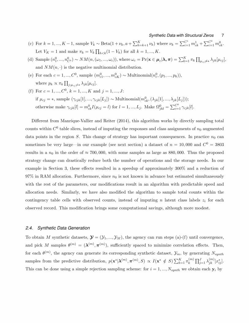
Figure 1 shows the resulting estimates using synthetic data from our TNPLCM and the comparison

approaches versus the true population values. We see that results from the TNPLCM line almost

perfectly within the main diagonal, indicating that these estimates are very close to their population

values (Figure 1a). In contrast, our comparison approach using sequential regression synthesis with

CART tuned with default parameters (Figure 1b) produces biased estimates, both overestimating and

underestimating. Our last comparison, fitting the NPLCM without truncating the support of the dis-

tribution (Figure 1c) illustrates the effect of the structural zeros. NPLCM estimates are relatively good,

although they exhibit a small but noticeable bias. However, the main difference with the TNPLCM

are a set of several estimates of population quantities (near the origin of Figure 1c) which should be

exactly zero, but are estimated with positive probability. These mostly result from structural zeros


0.0 0.1 0.2 0.3 0.4 0.5 0.6

0.0

0.1

0.2

0.3

0.4

0.5

0.6

Population Value

Syn

thet

ic −

TN

PLC

M

(a) TNPLCM

0.0 0.1 0.2 0.3 0.4 0.5 0.6

0.0

0.1

0.2

0.3

0.4

0.5

0.6

Population Value

Syn

thet

ic −

CA

RT

(b) CART

0.0 0.1 0.2 0.3 0.4 0.5 0.6

0.0

0.1

0.2

0.3

0.4

0.5

0.6

Population Value

Syn

thet

ic −

NP

LCM

(N

o st

ruct

ural

zer

os)

(c) NPLCM (no structural zeros)

Fig. 1: Mean estimates (over 200 experimental trials) of the test 3-way margin proportions estimatedfrom synthetic data vs. their actual population values (plots show a random sample of 2000 estimandsfor clarity).

being estimated with positive probability due to the lack of truncation of the support.

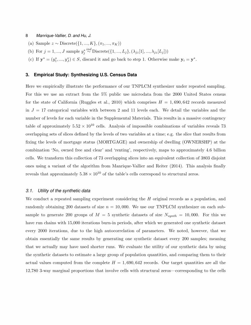
We have also computed the empirical coverage (over the 200 replications of the experiment) of 95%

intervals computed from the synthetic data, as well as from the original data for calibration. In this

comparison we have omitted the structural zeros, which in the case of the TNPLCM are not being

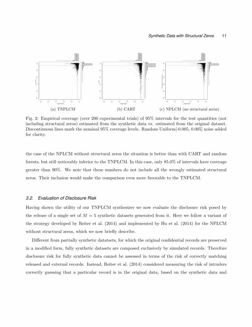
estimated—and are trivially set at their correct value of 0. Figure 2 shows these results. The coverage

obtained with the TNPLCM (Figure 2a) is comparable to that obtained using the original data, and

in general well within Monte Carlo error of their nominal value of 95%. In fact, 98.6% of the intervals

obtained from the TNPLCM have coverage above 80% (which is an even larger proportion than the

98.4% using the original data); moreover, 91% of the TNPLCM intervals have coverage above 90%

(c.f. 91.8% using original data). The coverage obtained using the comparison FCS synthesizers, using

CART and random forests is notably inferior (see online supplement for plots for the latter). In the

case of CART, 89.3% of intervals have coverage greater than 80%, and only 74.5% greater than 90%.

We note that in the case of CART it is possible to get much better utility by using a smaller con-

tamination parameter, although the disclosure risk properties of such procedure are somewhat dubious

(see Supplemental materials #2 for more information). Random forests fared much worse, with 64.3%

of intervals having coverage greater than 80% and 49.3% of them with coverage larger than 90%. In


1

TLC

MC

R1 Original Data Index

NU

LL

Index

NU

LL

0.0 0.2 0.4 0.6 0.8 1.0

0.0

0.2

0.4

0.6

0.8

1.0

x

y

(a) TNPLCM

1

CA

RT

1 Original Data Index

NU

LL

Index

NU

LL

0.0 0.2 0.4 0.6 0.8 1.00.

00.

20.

40.

60.

81.

0

x

y

(b) CART

1

LCM

CR

(N

o st

ruct

ural

zer

os)

1 Original Data Index

NU

LL

Index

NU

LL

0.0 0.2 0.4 0.6 0.8 1.0

0.0

0.2

0.4

0.6

0.8

1.0

x

y

(c) NPLCM (no structural zeros)

Fig. 2: Empirical coverage (over 200 experimental trials) of 95% intervals for the test quantities (notincluding structural zeros) estimated from the synthetic data vs. estimated from the original dataset.Discontinuous lines mark the nominal 95% coverage levels. Random Uniform[-0.005, 0.005] noise addedfor clarity.

the case of the NPLCM without structural zeros the situation is better than with CART and random

forests, but still noticeably inferior to the TNPLCM. In this case, only 85.0% of intervals have coverage

greater than 90%. We note that these numbers do not include all the wrongly estimated structural

zeros. Their inclusion would make the comparison even more favorable to the TNPLCM.

3.2. Evaluation of Disclosure Risk

Having shown the utility of our TNPLCM synthesizer we now evaluate the disclosure risk posed by

the release of a single set of M = 5 synthetic datasets generated from it. Here we follow a variant of

the strategy developed by Reiter et al. (2014) and implemented by Hu et al. (2014) for the NPLCM

without structural zeros, which we now briefly describe.

Different from partially synthetic datatsets, for which the original confidential records are preserved

in a modified form, fully synthetic datasets are composed exclusively by simulated records. Therefore

disclosure risk for fully synthetic data cannot be assessed in terms of the risk of correctly matching

released and external records. Instead, Reiter et al. (2014) considered measuring the risk of intruders

correctly guessing that a particular record is in the original data, based on the synthetic data and


additional information. More specifically, they proposed to evaluate and compare probabilities of

the form ρi(x) = p(x|Y ,X−i,K) ∝ p(Y |x,X−i,K)p(x|X−i,K), where Y = (Y1, . . . ,YM ) is the set

of all released synthetic datasets, X−i is the original data except for the i-th record, and K is the

knowledge of the intruder about the process that generated Y . Given an original record xi, ρi(x) is

the probability that an intruder who possesses the entire original dataset except for the i-th record,

guesses that the missing value is x. Therefore, whenever ρi(xi) ranks at the top (or among the top)

of the set ρi(x)x∈U(xi) where U(xi) is a set of suitable alternative candidates, we can consider the

record at risk. We repeat this procedure for all unique responses in the original sample; non unique

responses are already known to the intruder. We note that this is an extremely conservative approach,

as it is unlikely that actual intruders will ever have such detailed knowledge of the original sample. The

purpose of such evaluation is to obtain a sort of upper bound for the risks.

As Reiter et al. (2014) recommends, for each xi we take U(xi) to be the set of all responses that

result from varying one single value from xi at a time. This results in sets of∑

j Lj potential guesses,

from which we remove the structural zeros. We assume that the intruders know the set of structural

zeros, S, and the fact that Y was generated from the TNPLCM. Additionally we assume that intruders

do not have any a priori preference for particular guesses as long as they correspond to valid answers.

Thus we take p(x|X−i,K) ∝ 1x /∈ S. As the Associate Editor pointed out, other sensible prior

specifications could be employed here. In particular, intruders could base their prior distribution on

the observed frequencies in X−i. Such prior, however, would underweight sample uniques (which cannot

be present in X−i) resulting in less conservative disclosure risk measures. We direct readers to Reiter

et al. (2014) for further discussion about prior specifications and their effect.

We follow Hu et al. (2014) in computing the disclosure risks using an importance sampling approach,

recycling posterior samples from the TNPLCM’s parameters obtained from the MCMC algorithm. We

note, however, that these computations entail considerable difficulties. In our implementation we have

been unable to compute the actual guessing probabilities; we resorted instead to an indirect bootstrap

hypothesis testing framework aimed at approximating the ranking of each ρi(xi) among its comparison

class, U(xi). We detail our full procedure in Appendix 1.

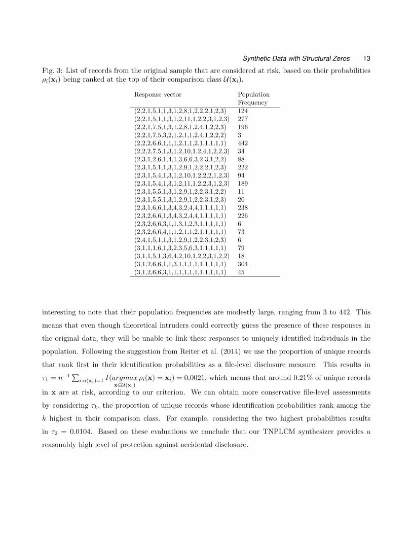
Table 3 shows the 21 records that we have evaluated to be at risk, based on their ranking at the top

of their corresponding comparison class. All these records are sample uniques by design. However it is


Fig. 3: List of records from the original sample that are considered at risk, based on their probabilitiesρi(xi) being ranked at the top of their comparison class U(xi).

Response vector PopulationFrequency

(2,2,1,5,1,1,3,1,2,8,1,2,2,2,1,2,3) 124(2,2,1,5,1,1,3,1,2,11,1,2,2,3,1,2,3) 277(2,2,1,7,5,1,3,1,2,8,1,2,4,1,2,2,3) 196(2,2,1,7,5,3,2,1,2,1,1,2,4,1,2,2,2) 3(2,2,2,6,6,1,1,1,2,1,1,2,1,1,1,1,1) 442(2,2,2,7,5,1,3,1,2,10,1,2,4,1,2,2,3) 34(2,3,1,2,6,1,4,1,3,6,6,3,2,3,1,2,2) 88(2,3,1,5,1,1,3,1,2,9,1,2,2,2,1,2,3) 222(2,3,1,5,4,1,3,1,2,10,1,2,2,2,1,2,3) 94(2,3,1,5,4,1,3,1,2,11,1,2,2,3,1,2,3) 189(2,3,1,5,5,1,3,1,2,9,1,2,2,3,1,2,2) 11(2,3,1,5,5,1,3,1,2,9,1,2,2,3,1,2,3) 20(2,3,1,6,6,1,3,4,3,2,4,4,1,1,1,1,1) 238(2,3,2,6,6,1,3,4,3,2,4,4,1,1,1,1,1) 226(2,3,2,6,6,3,1,1,3,1,2,3,1,1,1,1,1) 6(2,3,2,6,6,4,1,1,2,1,1,2,1,1,1,1,1) 73(2,4,1,5,1,1,3,1,2,9,1,2,2,3,1,2,3) 6(3,1,1,1,6,1,3,2,3,5,6,3,1,1,1,1,1) 79(3,1,1,5,1,3,6,4,2,10,1,2,2,3,1,2,2) 18(3,1,2,6,6,1,1,3,1,1,1,1,1,1,1,1,1) 304(3,1,2,6,6,3,1,1,1,1,1,1,1,1,1,1,1) 45

interesting to note that their population frequencies are modestly large, ranging from 3 to 442. This

means that even though theoretical intruders could correctly guess the presence of these responses in

the original data, they will be unable to link these responses to uniquely identified individuals in the

population. Following the suggestion from Reiter et al. (2014) we use the proportion of unique records

that rank first in their identification probabilities as a file-level disclosure measure. This results in

τ1 = n−1∑

i:n(xi)=1 I(argmaxx∈U(xi)

ρi(x) = xi) = 0.0021, which means that around 0.21% of unique records

in x are at risk, according to our criterion. We can obtain more conservative file-level assessments

by considering τk, the proportion of unique records whose identification probabilities rank among the

k highest in their comparison class. For example, considering the two highest probabilities results

in τ2 = 0.0104. Based on these evaluations we conclude that our TNPLCM synthesizer provides a

reasonably high level of protection against accidental disclosure.


4. Discussion

The TNPLCM is a promising tool for agencies seeking to generate high-utility multivariate categorical

synthetic data that can be shared with the public at a low disclosure risk. In our tests, using real

data from a 17-variable extract of the 2000 U.S. Census involving contingency tables with more than

5.5×1010 cells and more than 5.2×1010 structural zeros, the TNPLCM synthesizer did an excellent job

at preserving inferences for a battery of more than 12,000 population quantities, while simultaneously

enforcing the structural zero restrictions. The TNPLCM clearly outperformed the comparison methods

based on FCS using CART, random forests and plain NPLCM in terms of utility. Furthermore, our

evaluation of the disclosure risk indicates that in our example synthetic samples generated from the

TNPLCM posed a low disclosure risk.

We believe that the TNPCLM’s ability of seamlessly handling complex and extremely large sets

structural zeros in both model fitting and synthetic data generation is currently unmatched by other

synthetic data generation proposals. In particular, being a joint probability modeling method, it is

immune to several limitations of FCS-based methods. One of such limitations, which has not received

much attention in the literature, is the fact that some patterns of structural zeros can cause FCS

synthesizers to fail producing samples from certain regions of the support of the distribution. Specif-

ically, since FCS approaches work by updating one variable at a time while keeping the rest fixed,

reaching any point that differs by more than one coordinate from the current position requires passing

through intermediate points in the support. However, if those intermediate points are all structural

zeros, reaching that destination from the current position would be impossible, effectively leading to a

reducible Markov Chain. As a simple but non-trivial example consider a survey with binary variables

so that C = 1, 2J , where structural restrictions state that x1 cannot be equal to x2. Under such

configuration, a FCS synthesizer that starts on any value where (x1, x2) = (1, 2) cannot sample values

where (x1, x2) = (2, 1), since doing so would require passing through either (1, 1) or (2, 2), which are

structural zeros. The same considerations apply if the starting point were such that (x1, x2) = (2, 1).

We can construct more complex examples if we consider variables with more than two levels. We note

that this behavior is restricted to strict FCS approaches (e.g Reiter, 2005; Matthews et al., 2010), and

is a direct consequence of the particular way in which strict FCS approaches work: by sequentially

regressing one variable at a time conditional on the current value of the rest of the multivariate vector.


The TNPLCM, in contrast, does not suffer such limitation as it can just sample all the coordinates at

a time.

Our MCMC sampler for the TNPLCM is computationally efficient and requires small to no tuning

from the users. In our examples, our algorithm took approximately 375 seconds to generate a set

of M = 5 synthetic datasets of size n = 10, 000 using a standard desktop computer. Moreover, our

improvements over Manrique-Vallier and Reiter (2014) result in a drastic reduction, on the order of 97%,

of memory allocation needs. Such level of computational efficiency is crucial in synthetic data generation

applications. Real-life datasets of the type agencies are interested in synthesizing are usually generally

large and highly multivariate. Synthesis methods should be able to scale appropriately. Therefore

we believe that our proposal should be an attractive candidate for routine real-life applications by

statistical agencies and other organizations that wish to disseminate sensitive data. We further note

that future implementations of our algorithm can achieve even greater speeds by exploiting parallelism.

In particular, steps 1, 5 and 6 in the algorithm described in Section 2.3 involve the sampling of large

numbers of (conditionally) independent multinomial variates, all of which can be done in parallel.

Acknowledgments

The authors thank Jerry Reiter and Arturo Valdivia for valuable suggestions.

References

Benjamini, Y. and Hochberg, Y. (1995) Controlling the false discovery rate: a practical and powerful

approach to multiple testing. Journal of the Royal Statistical Society. Series B (Methodological),

289–300.

Bishop, Y., Fienberg, S. and Holland, P. (1975) Discrete Multivariate Analysis: Theory and Practice.

Cambridge, MA: MIT Press. Reprinted in 2007 by Springer-Verlag, New York.

Caiola, G. and Reiter, J. P. (2010) Random forests for generating partially synthetic, categorical data.

Transactions on Data Privacy, 3, 27–42.


Drechsler, J. and Reiter, J. P. (2011) An empirical evaluation of easily implemented, nonparametric

methods for generating synthetic datasets. Computational Statistics & Data Analysis, 55, 3232–3243.

Dunson, D. and Xing, C. (2009) Nonparametric bayes modeling of multivariate categorical data. Journal

of the American Statistical Association, 104, 1042–1051.

Goodman, L. A. (1974) Exploratory latent structure analysis using both identifiable and unidentifiable

models. Biometrika, 61, 215–231.

Hu, J., Reiter, J. P. and Wang, Q. (2014) Disclosure risk evaluation for fully synthetic categorical data.

In Privacy in Statistical Databases (ed. J. Domingo-Ferrer), no. 8744 in Lecture Notes in Computer

Science, 185–199. Heidelberg: Springer.

Ishwaran, H. and James, L. F. (2001) Gibbs sampling for stick-breaking priors. Journal of the American

Statistical Association, 96, 161–173.

Manrique-Vallier, D. (2016) Bayesian population size estimation using dirichlet process mixtures. Bio-

metrics, 72, 1246–1254.

Manrique-Vallier, D. and Reiter, J. P. (2014) Bayesian estimation of discrete multivariate latent struc-

ture models with structural zeros. Journal of Computational and Graphical Statistics, 23, 1061–1079.

URL: http://dx.doi.org/10.1080/10618600.2013.844700.

— (to appear) Bayesian simultaneous edit and imputation for multivariate cate-

gorical data. Journal of the American Statistical Association, 0, 0–0. URL:

http://dx.doi.org/10.1080/01621459.2016.1231612.

Matthews, G. J., Harel, O. and Aseltine, R. H. (2010) Examining the robustness of fully synthetic data

techniques for data with binary variables. Journal of Statistical Computation and Simulation, 79,

609–624.

Raghunathan, T. E., Lepkowski, J. M., van Hoewyk, J. and Solenberger, P. (2001) A multivariate tech-

nique for multiply imputing missing values using a series of regression models. Survey Methodology,

27, 85–96.


Raghunathan, T. E., Reiter, J. P. and Rubin, D. B. (2003) Multiple imputation for statistical disclosure

limitation. Journal of Official Statistics, 19, 1–16.

Reiter, J. P. (2005) Using CART to generate partially synthetic, public use microdata. Journal of

Official Statistics, 21, 441–462.

Reiter, J. P. and Raghunathan, T. E. (2007) The multiple adaptations of multiple imputation. Journal

of the American Statistical Association, 102, 1462–1471.

Reiter, J. P., Wang, Q. and Zhang, B. (2014) Bayesian estimation of disclosure risks for multiply

imputed, synthetic data. Journal of Privacy and Confidentiality, 6, 2.

Robert, C. and Casella, G. (2004) Monte Carlo Statistical Methods. New York: Springer-Verlag, 2nd

ed. edn.

Rubin, D. B. (1993) Statistical disclosure limitation. Journal of official Statistics, 9, 461–468.

Ruggles, S., Alexander, T., Genadek, K., Goeken, R., Schroeder, M. B. and Sobek, M. (2010) Inte-

grated public use microdata series: Version 5.0 [machine-readable database]. University of Minnesota,

Minneapolis. http://usa.ipums.org.

Sethuraman, J. (1994) A constructive definition of Dirichlet priors. Statistica Sinica, 4, 639–650.

Si, Y. and Reiter, J. P. (2013) Nonparametric Bayesian multiple imputation for incomplete categorical

variables in large-scale assessment surveys. Journal of Educational and Behavioral Statistics, 38,

499–521.

Van Buuren, S., Brand, J. P., Groothuis-Oudshoorn, C. G. and Rubin, D. B. (2006) Fully conditional

specification in multivariate imputation. Journal of Statistical Computation and Simulation, 76,

1049–1064. URL: http://dx.doi.org/10.1080/10629360600810434.

Van Buuren, S. and Oudshoorn, C. (1999) Flexible multivariate imputation by MICE. Tech. rep.,

Leiden: TNO Preventie en Gezondheid, TNO/VGZ/PG 99.054.

Vermunt, J. K., Ginkel, J. R. V., der Ark, L. A. V. and Sijtsma, K. (2008) Multiple imputation of

incomplete categorical data using latent class analysis. Sociological Methodology, 38, 369–397.


White, I. R., Royston, P. and Wood, A. M. (2011) Multiple imputation using chained equa-

tions: Issues and guidance for practice. Statistics in Medicine, 30, 377–399. URL:

http://dx.doi.org/10.1002/sim.4067.

Appendix: Computation of disclosure risk

Following Hu et al. (2014) we note that evaluating the disclosure risk of a single unique combination

xi from the original sample involves obtaining the probabilities

p(x|Y ,X−i,K) ∝M∏m=1

∫p(Ym|X x

−i,K, θ)p(θ|X x−i,K)dθ × p(x|X−i,K) (6)

for all potential guesses x (including xi) in a comparison class U(xi) ⊂ C \ S. Here Ym is the m-th

synthetic dataset, X−i is the original data without its i-th element, X x−i is the dataset that results from

replacing the i-th element of X with x, and θ is the vector of parameters from the TNPLCM. As noted

in Section 3.2 we assume that intruders do not have any preference a priori about records from U(xi)

so p(x|X−i,K) ∝ 1x /∈ S.

Hu et al. (2014) proposed approximating the M integrals in (6) through importance sampling, using

T samples obtained from the NPLCM posterior distribution conditional on the original data, p(θ|X ).

The resulting Monte Carlo approximation for the TNPLCM is:

∫p(Ym|X x

−i,K, θ)p(θ|X x−i,K)dθ = Eθ[L(θ;Ym)|X x

−i] ≈T∑t=1

w(t;xi,x)L(θ(t);Ym) (7)

where L(θ;Ym) =∏

x∈YmfTNPLCM (x|θ), and w(t;xi,x) are self-normalized importance weights w(t;xi,x) ∝

fTNPCLM (x|θ(t))/fTNPCLM (xi|θ(t)) such that∑

tw(t;xi,x) = 1 (see Robert and Casella, 2004, p.95).

Unfortunately, the resulting estimator in (7) has serious stability issues which makes it unsuitable for

risk calculations. In particular, values of L(θ(t);Ym) vary by several thousands in the log scale from one

sample θ(t) to another, resulting in an estimator with an enormous mean squared error. As an alternative

we propose to estimate the distribution of g(θ) = logL(θ;Ym), for θ ∼ p(θ|X x−i,K), by assuming that

it belongs to a simple parametric family with density h(·|φ), so that we can compute the expectation

E[exp g(θ)|φ] analytically. Inspection of the samples from g(θ), using importance re-sampling, suggest


that a normal approximation might be adequate. However, since the behavior of exp g(θ) is heavily

influenced by the assumptions about the right tail of the distribution, and the log-likelihood must be

upper-bounded by zero, we instead opted for assuming that −g(θ) ∼ Gamma(·|a, b), where E[−g(θ)] =

a/b, so that logE[exp g(θ)|a, b] = −a log(1 + 1/b). We note that assuming that g(θ) follows a normal

distribution results in the same conclusions about the ranking of probabilities. We obtain a method

of moments estimator for a and b, by approximating the first and second moments of g(θ) using the

importance sampling estimators µ1 =∑

tw(t;xi,x)g(θ(t)) and µ2 =∑

tw(t;xi,x)g(θ(t))2.

An additional problem presents when we try to rank the resulting probabilities. Experiments suggest

that the variances of the resulting estimators, while much smaller than those obtained from the naive

approach from (7), are still considerable. Furthermore, since we compute all the probabilities from

the same posterior sample of θ, these estimates are correlated. For these reasons, instead of simply

considering a ranking of point estimators, we resort to a bootstrap approach whereby we consider the

joint sampling distribution of all the probabilities in the comparison set U(xi). We then compute

p-values for hypotheses H0(i, k) stating that the probability of guessing the true missing value, xi, is

among the largest k probabilities in U(xi). For example H0(i, 1) states that the probability associated

with xi is the largest in U(xi) or, equivalently, that the record is ranked first. Larger values of k

result in more conservative statements about the disclosure risk. Finally, when considering several xis

simultaneously (for example, when evaluating all the records in the original dataset) we need to account

for the possibility of false positives resulting from multiple comparisons. We account for this problem

by using the Benjamini and Hochberg (1995) procedure with a false discovery rate of 0.005, meaning

that we accept the risk that about 0.5% of the records deemed safe could actually be at risk.

Bayesian Non-parametric Generation of Fully Synthetic...

Documents

Transcript of Bayesian Non-parametric Generation of Fully Synthetic...