Bayesian Networks - cs.cmu.edumgormley/courses/10601bd-f18/slides/lecture21... · • A Bayesian...
57
Bayesian Networks 1 10-601 Introduction to Machine Learning Matt Gormley Lecture 21 Nov. 12, 2018 Machine Learning Department School of Computer Science Carnegie Mellon University
-
Upload
truonghuong -
Category
Documents
-
view
226 -
download
0
Transcript of Bayesian Networks - cs.cmu.edumgormley/courses/10601bd-f18/slides/lecture21... · • A Bayesian...

Bayesian Networks
1
10-601 Introduction to Machine Learning
Matt GormleyLecture 21
Nov. 12, 2018
Machine Learning DepartmentSchool of Computer ScienceCarnegie Mellon University

Reminders
• Homework 7: HMMs– Out: Wed, Nov 7– Due: Mon, Nov 19 at 11:59pm
• Schedule Changes– Lecture on Fri, Nov 16– Recitation on Mon, Nov 19
2

Peer Tutoring
3
Tutor Tutee

HIDDEN MARKOV MODELS
4

Derivation of Forward Algorithm
5
Derivation:
Definition:
Forward-Backward Algorithm
6

Viterbi Algorithm
7

Inference in HMMsWhat is the computational complexity of inference for HMMs?
• The naïve (brute force) computations for Evaluation, Decoding, and Marginals take exponential time, O(KT)
• The forward-backward algorithm and Viterbialgorithm run in polynomial time, O(T*K2)– Thanks to dynamic programming!
8

Shortcomings of Hidden Markov Models
• HMM models capture dependences between each state and only its corresponding observation – NLP example: In a sentence segmentation task, each segmental state may depend
not just on a single word (and the adjacent segmental stages), but also on the (non-local) features of the whole line such as line length, indentation, amount of white space, etc.
• Mismatch between learning objective function and prediction objective function– HMM learns a joint distribution of states and observations P(Y, X), but in a prediction
task, we need the conditional probability P(Y|X)
© Eric Xing @ CMU, 2005-2015 9
Y1 Y2 … … … Yn
X1 X2 … … … Xn
START

MBR DECODING
10
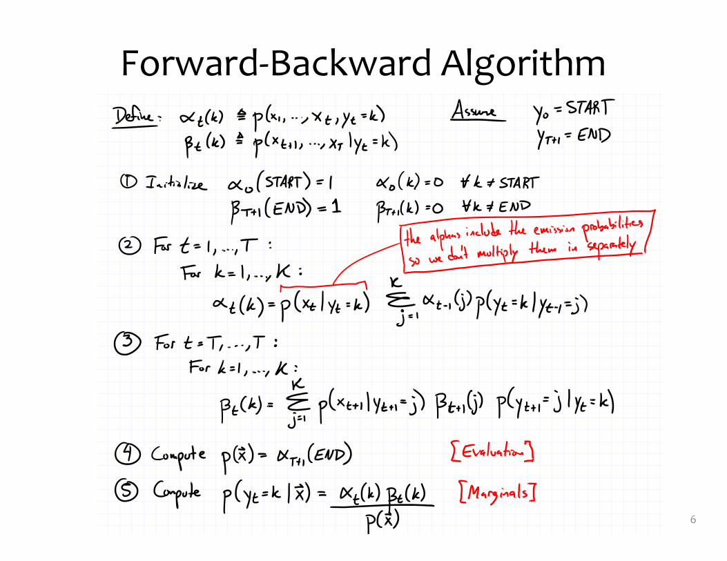
Inference for HMMs
– Three Inference Problems for an HMM1. Evaluation: Compute the probability of a given
sequence of observations2. Viterbi Decoding: Find the most-likely sequence of
hidden states, given a sequence of observations3. Marginals: Compute the marginal distribution for a
hidden state, given a sequence of observations4. MBR Decoding: Find the lowest loss sequence of
hidden states, given a sequence of observations (Viterbi decoding is a special case)
11
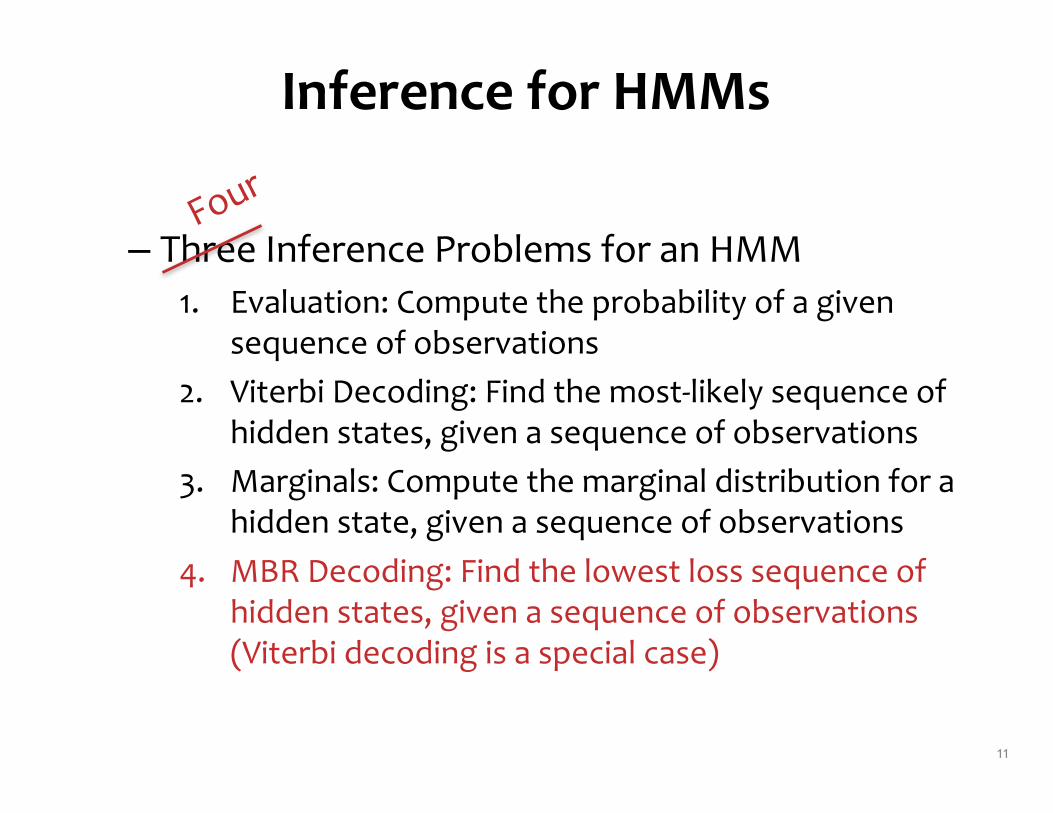
Minimum Bayes Risk Decoding• Suppose we given a loss function l(y’, y) and are
asked for a single tagging• How should we choose just one from our probability
distribution p(y|x)?• A minimum Bayes risk (MBR) decoder h(x) returns
the variable assignment with minimum expected loss under the model’s distribution
12
h✓
(x) = argminy
Ey⇠p✓(·|x)[`(y,y)]
= argminy
X
y
p✓
(y | x)`(y,y)
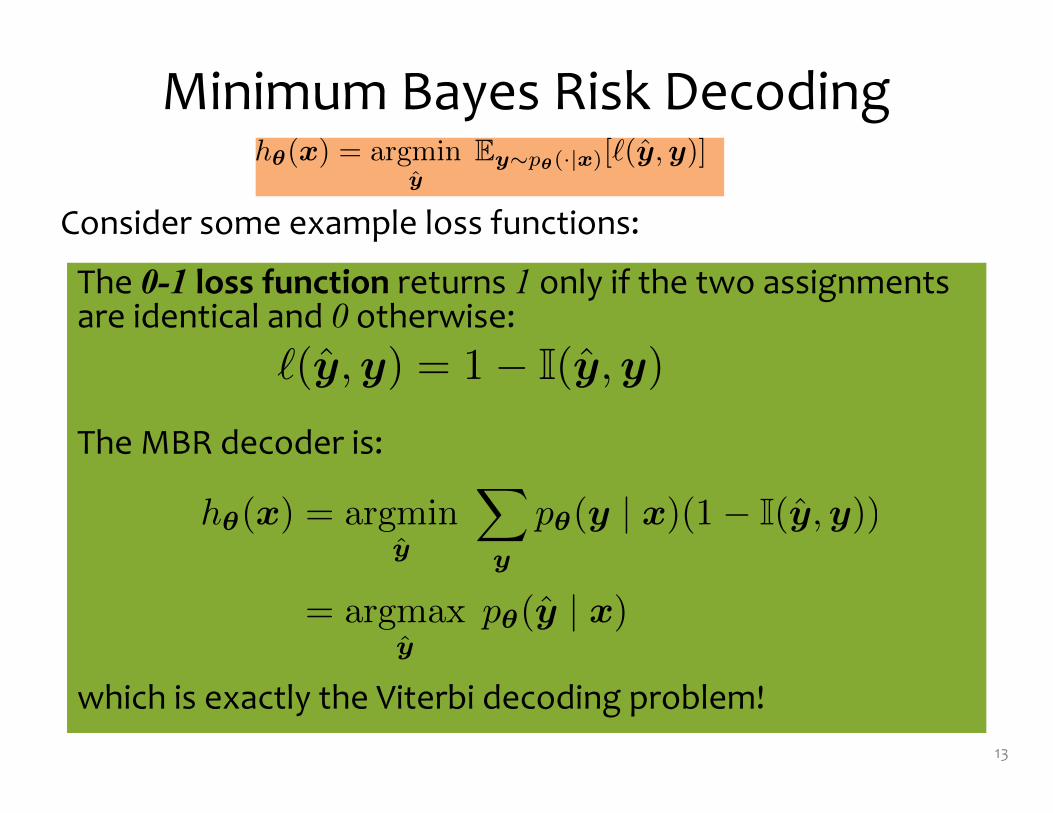
The 0-1 loss function returns 1 only if the two assignments are identical and 0 otherwise:
The MBR decoder is:
which is exactly the Viterbi decoding problem!
Minimum Bayes Risk Decoding
Consider some example loss functions:
13
`(y,y) = 1� I(y,y)
h✓(x) = argmin
y
X
y
p✓(y | x)(1� I(ˆy,y))
= argmax
yp✓(ˆy | x)
h✓
(x) = argminy
Ey⇠p✓(·|x)[`(y,y)]
= argminy
X
y
p✓
(y | x)`(y,y)
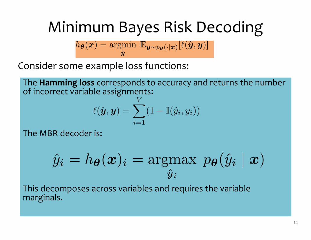
The Hamming loss corresponds to accuracy and returns the number of incorrect variable assignments:
The MBR decoder is:
This decomposes across variables and requires the variable marginals.
Minimum Bayes Risk Decoding
Consider some example loss functions:
14
`(y,y) =VX
i=1
(1� I(yi, yi))
yi = h✓(x)i = argmax
yi
p✓(yi | x)
h✓
(x) = argminy
Ey⇠p✓(·|x)[`(y,y)]
= argminy
X
y
p✓
(y | x)`(y,y)

BAYESIAN NETWORKS
15

Bayes Nets Outline• Motivation
– Structured Prediction• Background
– Conditional Independence– Chain Rule of Probability
• Directed Graphical Models– Writing Joint Distributions– Definition: Bayesian Network– Qualitative Specification– Quantitative Specification– Familiar Models as Bayes Nets
• Conditional Independence in Bayes Nets– Three case studies– D-separation– Markov blanket
• Learning– Fully Observed Bayes Net– (Partially Observed Bayes Net)
• Inference– Background: Marginal Probability– Sampling directly from the joint distribution– Gibbs Sampling
17
DIRECTED GRAPHICAL MODELSBayesian Networks
18
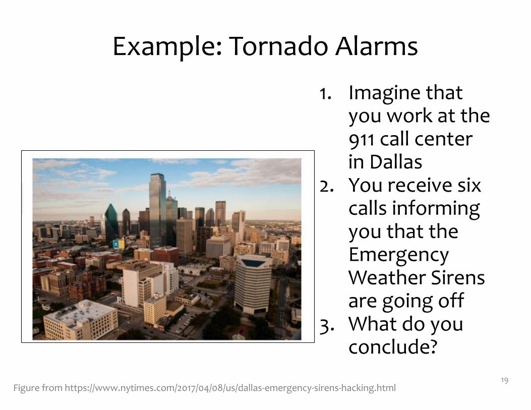
Example: Tornado Alarms1. Imagine that
you work at the 911 call center in Dallas
2. You receive six calls informing you that the Emergency Weather Sirens are going off
3. What do you conclude?
19Figure from https://www.nytimes.com/2017/04/08/us/dallas-emergency-sirens-hacking.html
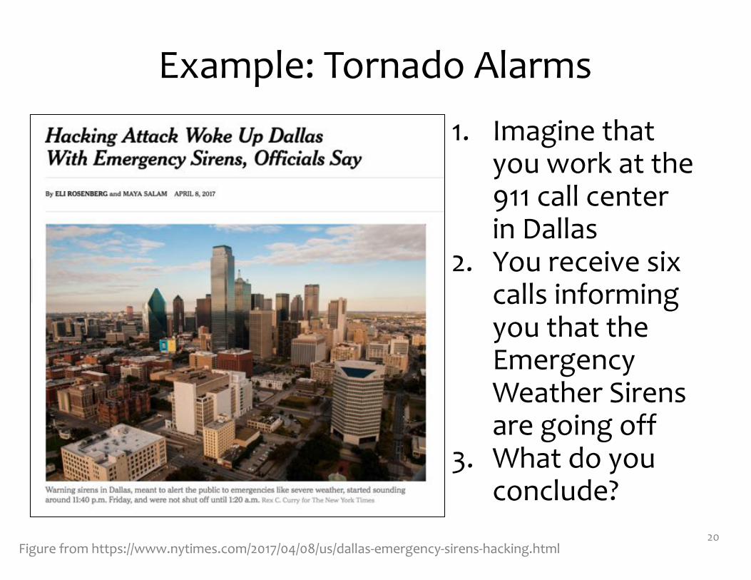
Example: Tornado Alarms1. Imagine that
you work at the 911 call center in Dallas
2. You receive six calls informing you that the Emergency Weather Sirens are going off
3. What do you conclude?
20Figure from https://www.nytimes.com/2017/04/08/us/dallas-emergency-sirens-hacking.html
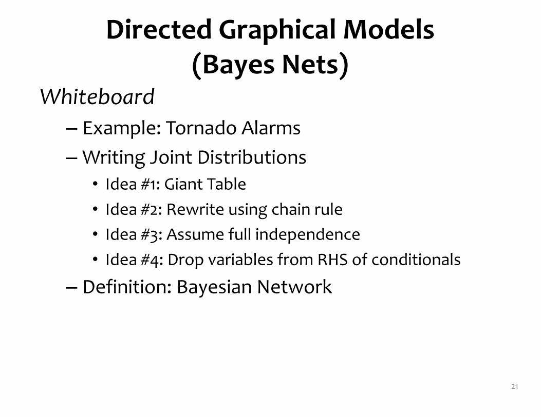
Directed Graphical Models (Bayes Nets)
Whiteboard– Example: Tornado Alarms– Writing Joint Distributions• Idea #1: Giant Table• Idea #2: Rewrite using chain rule• Idea #3: Assume full independence• Idea #4: Drop variables from RHS of conditionals
– Definition: Bayesian Network
21

Bayesian Network
22
p(X1, X2, X3, X4, X5) =
p(X5|X3)p(X4|X2, X3)
p(X3)p(X2|X1)p(X1)
X1
X3X2
X4 X5
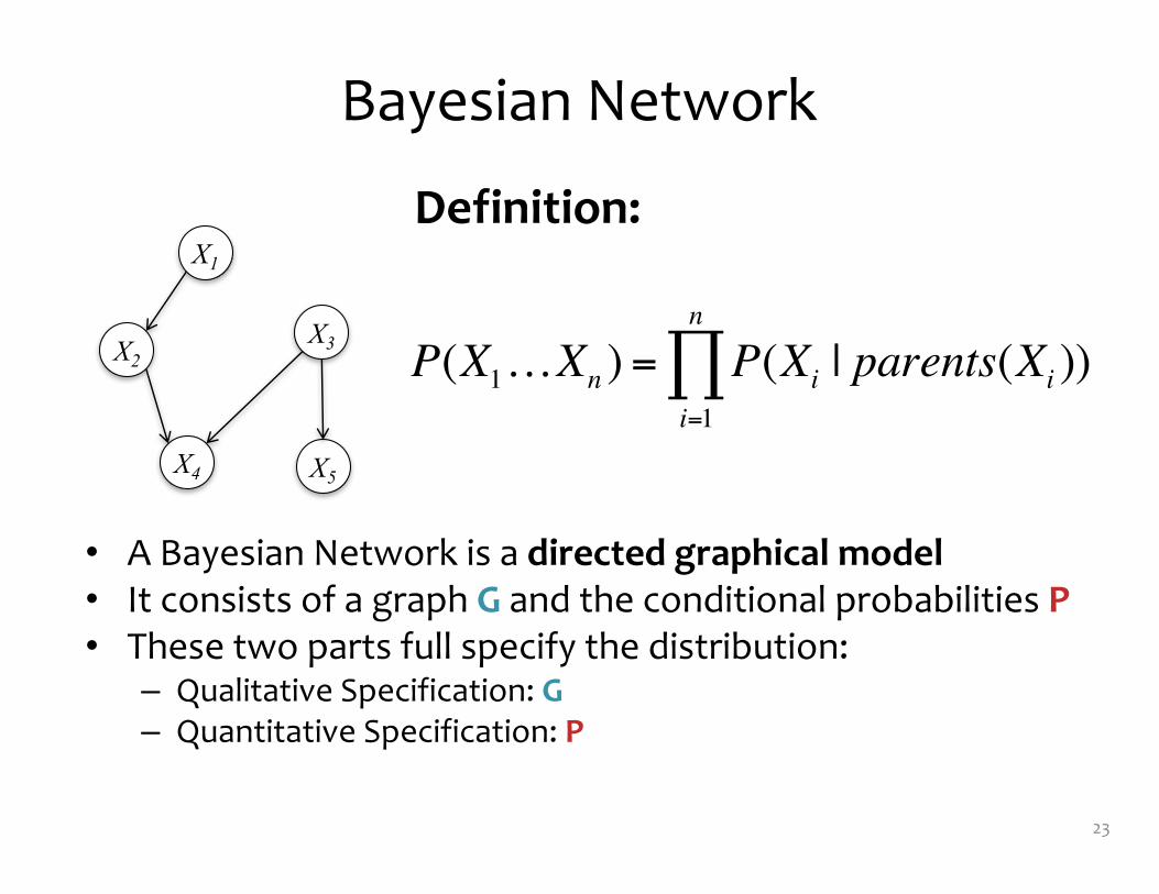
Bayesian Network
• A Bayesian Network is a directed graphical model• It consists of a graph G and the conditional probabilities P• These two parts full specify the distribution:
– Qualitative Specification: G– Quantitative Specification: P
23
X1
X3X2
X4 X5
Definition:
P(X1…Xn ) = P(Xi | parents(Xi ))i=1
n
∏

Qualitative Specification
• Where does the qualitative specification come from?
– Prior knowledge of causal relationships– Prior knowledge of modular relationships– Assessment from experts– Learning from data (i.e. structure learning)– We simply link a certain architecture (e.g. a
layered graph) – …
© Eric Xing @ CMU, 2006-2011 24

a0 0.75a1 0.25
b0 0.33b1 0.67
a0b0 a0b1 a1b0 a1b1
c0 0.45 1 0.9 0.7c1 0.55 0 0.1 0.3
A B
C
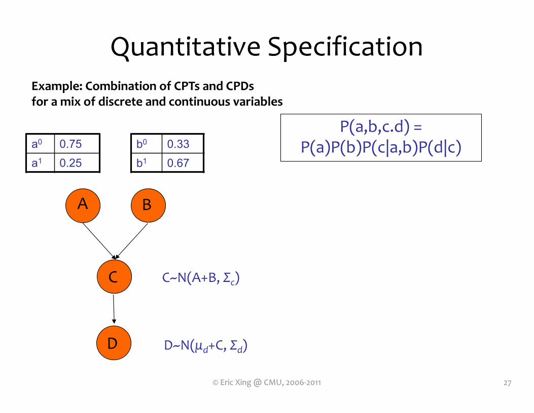
P(a,b,c.d) = P(a)P(b)P(c|a,b)P(d|c)
Dc0 c1
d0 0.3 0.5d1 07 0.5
Quantitative Specification
25© Eric Xing @ CMU, 2006-2011
Example: Conditional probability tables (CPTs)for discrete random variables
A B
C
P(a,b,c.d) = P(a)P(b)P(c|a,b)P(d|c)
D
A~N(μa, Σa) B~N(μb, Σb)
C~N(A+B, Σc)
D~N(μd+C, Σd)D
C
P(D|
C)
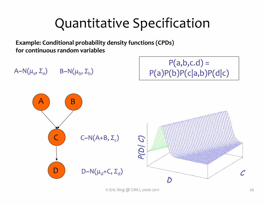
Quantitative Specification
26© Eric Xing @ CMU, 2006-2011
Example: Conditional probability density functions (CPDs)for continuous random variables
A B
C
P(a,b,c.d) = P(a)P(b)P(c|a,b)P(d|c)
D
C~N(A+B, Σc)
D~N(μd+C, Σd)
Quantitative Specification
27© Eric Xing @ CMU, 2006-2011
Example: Combination of CPTs and CPDs for a mix of discrete and continuous variables
a0 0.75a1 0.25
b0 0.33b1 0.67
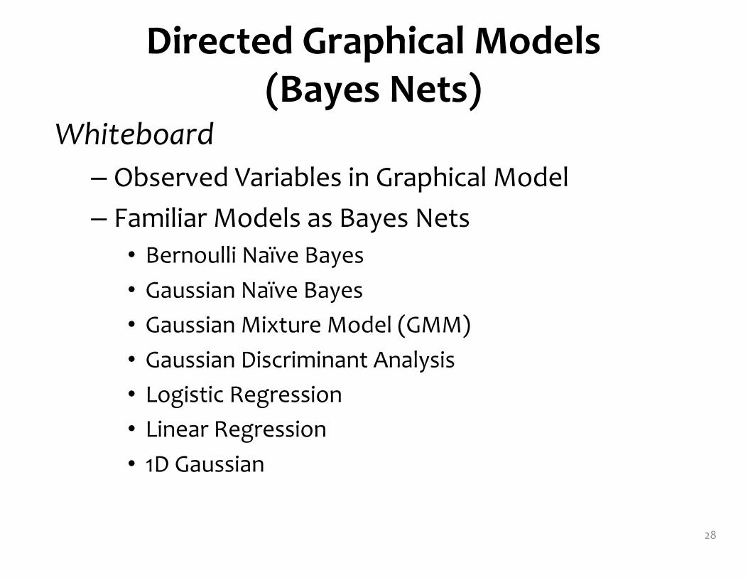
Directed Graphical Models (Bayes Nets)
Whiteboard– Observed Variables in Graphical Model– Familiar Models as Bayes Nets• Bernoulli Naïve Bayes• Gaussian Naïve Bayes• Gaussian Mixture Model (GMM)• Gaussian Discriminant Analysis• Logistic Regression• Linear Regression• 1D Gaussian
28
GRAPHICAL MODELS:DETERMINING CONDITIONAL INDEPENDENCIES
Slide from William Cohen
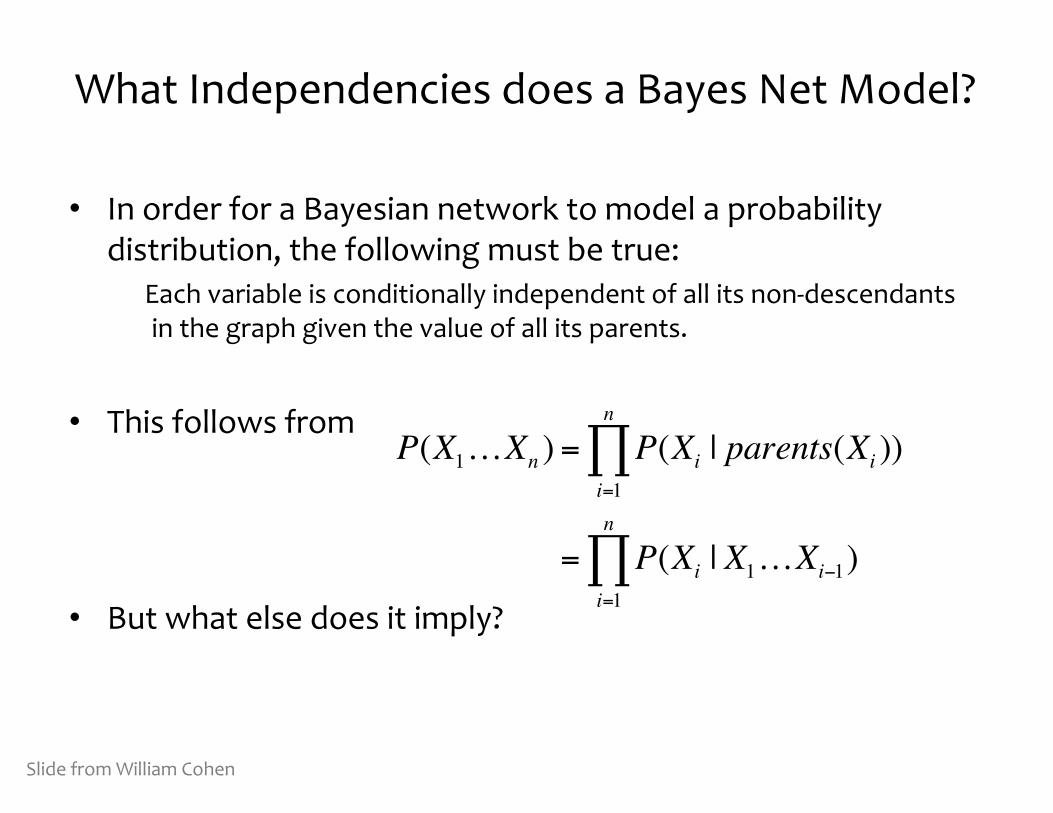
What Independencies does a Bayes Net Model?
• In order for a Bayesian network to model a probability distribution, the following must be true:
Each variable is conditionally independent of all its non-descendants in the graph given the value of all its parents.
• This follows from
• But what else does it imply?
P(X1…Xn ) = P(Xi | parents(Xi ))i=1
n
∏
= P(Xi | X1…Xi−1)i=1
n
∏
Slide from William Cohen
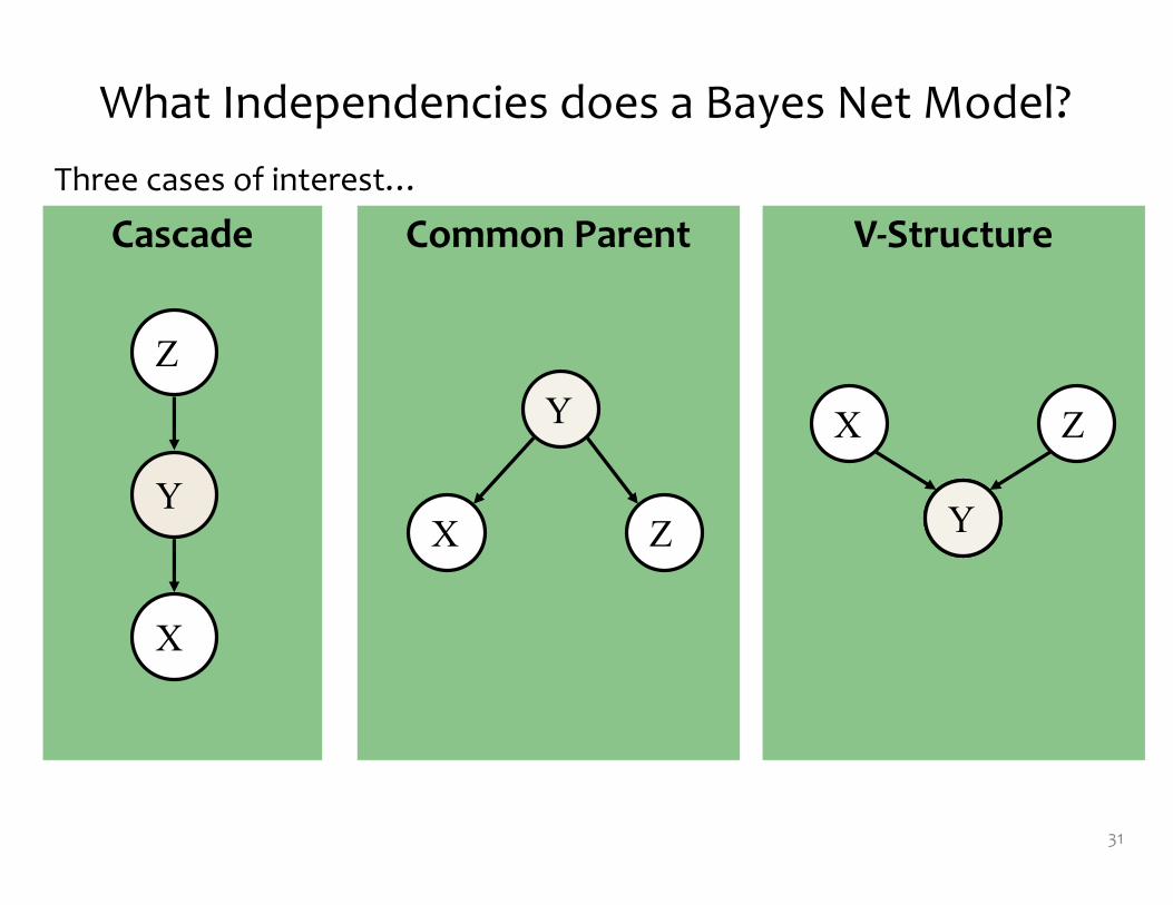
Common Parent V-StructureCascade
What Independencies does a Bayes Net Model?
31
Three cases of interest…
Z
Y
X
Y
X Z
ZX
YY
Common Parent V-StructureCascade
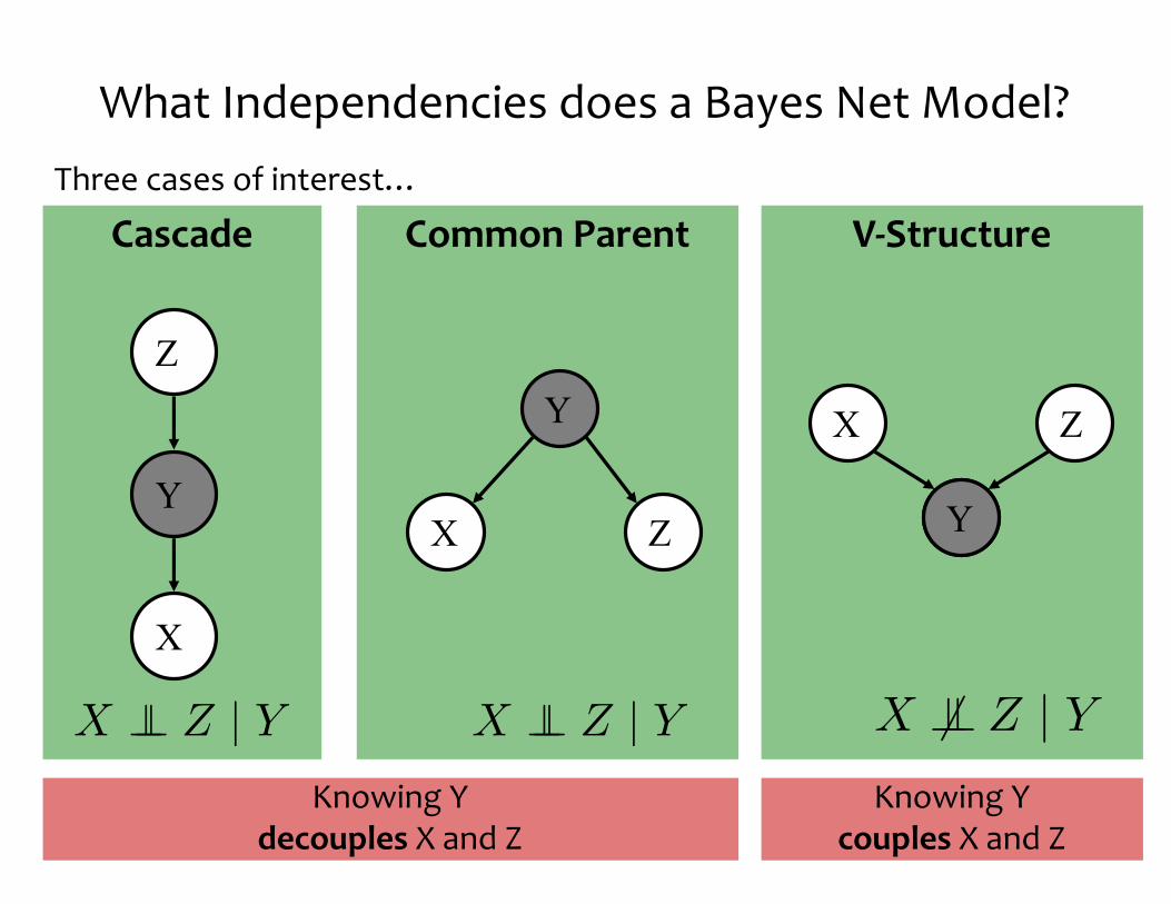
What Independencies does a Bayes Net Model?
32
Z
Y
X
Y
X Z
ZX
YY
X �� Z | Y X �� Z | Y X ��� Z | Y
Knowing Y decouples X and Z
Knowing Y couples X and Z
Three cases of interest…
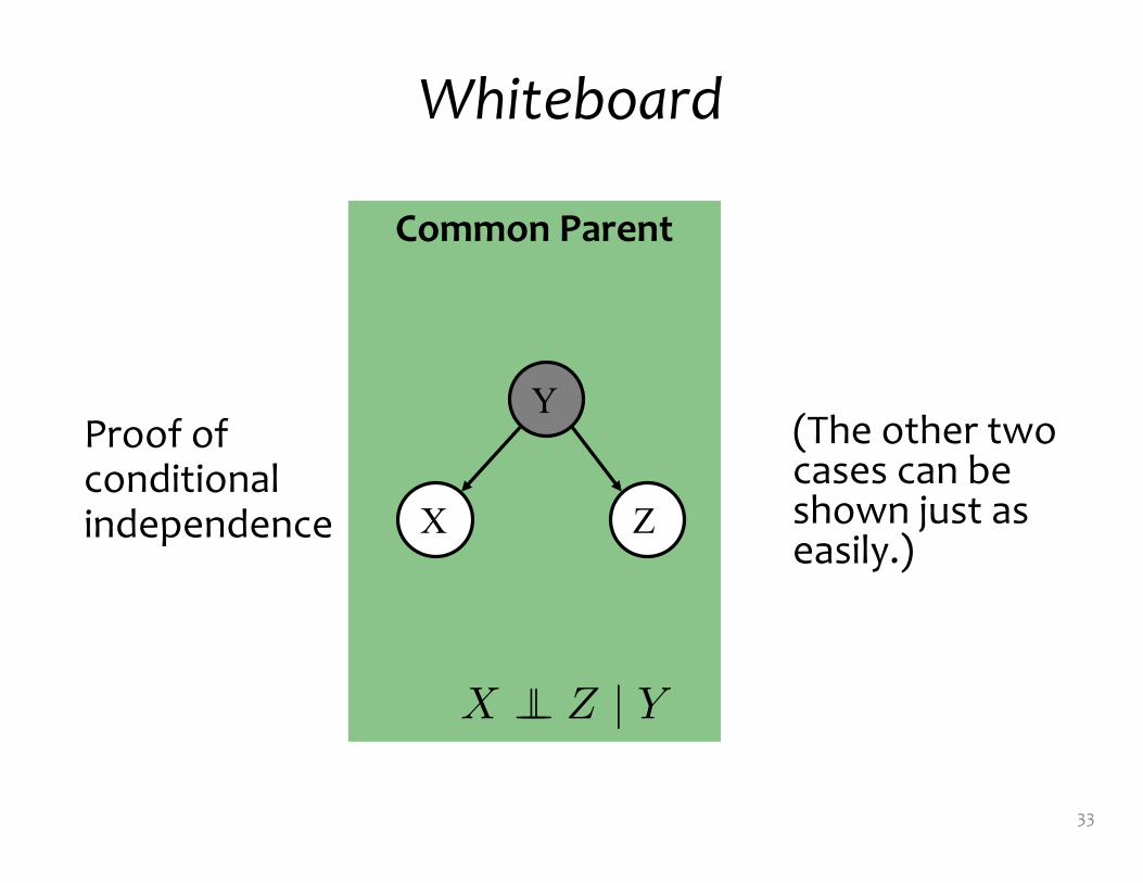
Whiteboard
(The other two cases can be shown just as easily.)
33
Common Parent
Y
X Z
X �� Z | Y
Proof of conditional independence
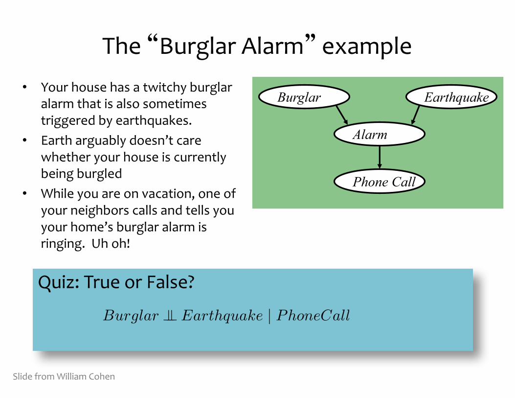
The �Burglar Alarm� example• Your house has a twitchy burglar
alarm that is also sometimes triggered by earthquakes.
• Earth arguably doesn’t care whether your house is currently being burgled
• While you are on vacation, one of your neighbors calls and tells you your home’s burglar alarm is ringing. Uh oh!
Burglar Earthquake
Alarm
Phone Call
Slide from William Cohen
Quiz: True or False?
Burglar �� Earthquake | PhoneCall

Markov Blanket
36
Def: the Markov Blanket of a node is the set containing the node’s parents, children, and co-parents.
Def: the co-parents of a node are the parents of its children
Thm: a node is conditionally independent of every other node in the graph given its Markov blanket
X1
X4X3
X6 X7
X9
X12
X5
X2
X8
X10
X13
X11
Markov Blanket
37
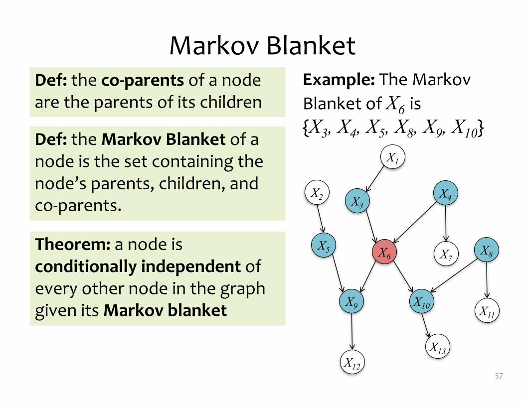
Def: the Markov Blanket of a node is the set containing the node’s parents, children, and co-parents.
Def: the co-parents of a node are the parents of its children
Theorem: a node is conditionally independent of every other node in the graph given its Markov blanket
X1
X4X3
X6 X7
X9
X12
X5
X2
X8
X10
X13
X11
Example: The Markov Blanket of X6 is {X3, X4, X5, X8, X9, X10}
Markov Blanket
38
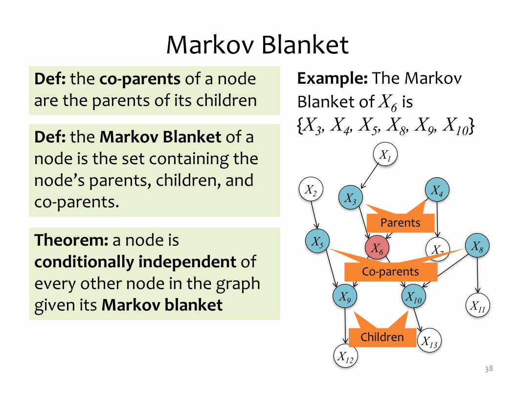
Def: the Markov Blanket of a node is the set containing the node’s parents, children, and co-parents.
Def: the co-parents of a node are the parents of its children
Theorem: a node is conditionally independent of every other node in the graph given its Markov blanket
X1
X4X3
X6 X7
X9
X12
X5
X2
X8
X10
X13
X11
Example: The Markov Blanket of X6 is {X3, X4, X5, X8, X9, X10}
ParentsChildren
ParentsCo-parents
ParentsParents
D-Separation
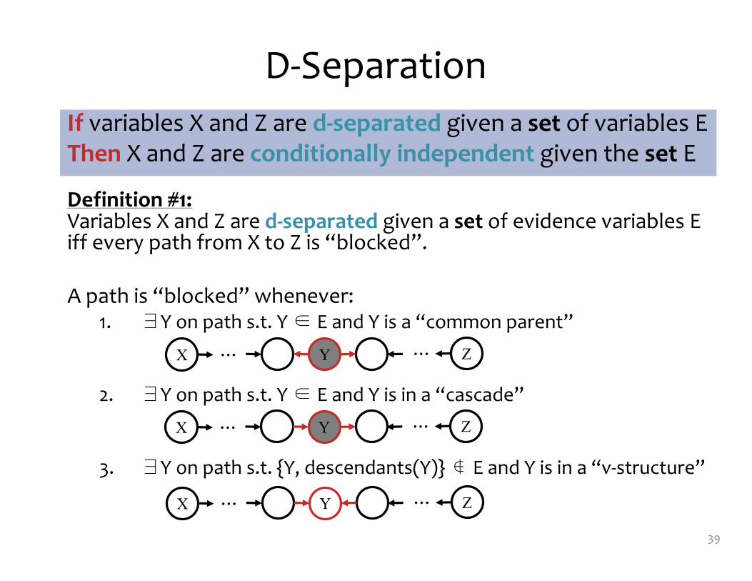
Definition #1: Variables X and Z are d-separated given a set of evidence variables E iff every path from X to Z is “blocked”.
A path is “blocked” whenever:1. �Y on path s.t. Y � E and Y is a “common parent”
2. �Y on path s.t. Y � E and Y is in a “cascade”
3. �Y on path s.t. {Y, descendants(Y)} � E and Y is in a “v-structure”
39
If variables X and Z are d-separated given a set of variables EThen X and Z are conditionally independent given the set E
YX Z… …
YX Z… …
YX Z… …

D-Separation
Definition #2: Variables X and Z are d-separated given a set of evidence variables E iff there does not exist a path in the undirected ancestral moral graph with E removed.
1. Ancestral graph: keep only X, Z, E and their ancestors2. Moral graph: add undirected edge between all pairs of each node’s parents3. Undirected graph: convert all directed edges to undirected4. Givens Removed: delete any nodes in E
40
If variables X and Z are d-separated given a set of variables EThen X and Z are conditionally independent given the set E
�A and B connected� not d-separated
A B
C
D E
F
Original:
A B
C
D E
Ancestral:
A B
C
D E
Moral:
A B
C
D E
Undirected:
A B
C
Givens Removed:Example Query: A ⫫ B | {D, E}
SUPERVISED LEARNING FOR BAYES NETS
41
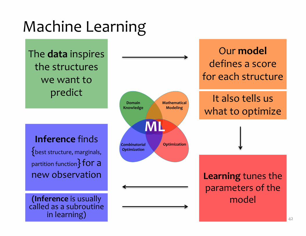
Machine Learning
42
The data inspires the structures
we want to predict It also tells us
what to optimize
Our modeldefines a score
for each structure
Learning tunes the parameters of the
model
Inference finds {best structure, marginals,
partition function} for a new observation
Domain Knowledge
Mathematical Modeling
OptimizationCombinatorial Optimization
ML
(Inference is usually called as a subroutine
in learning)
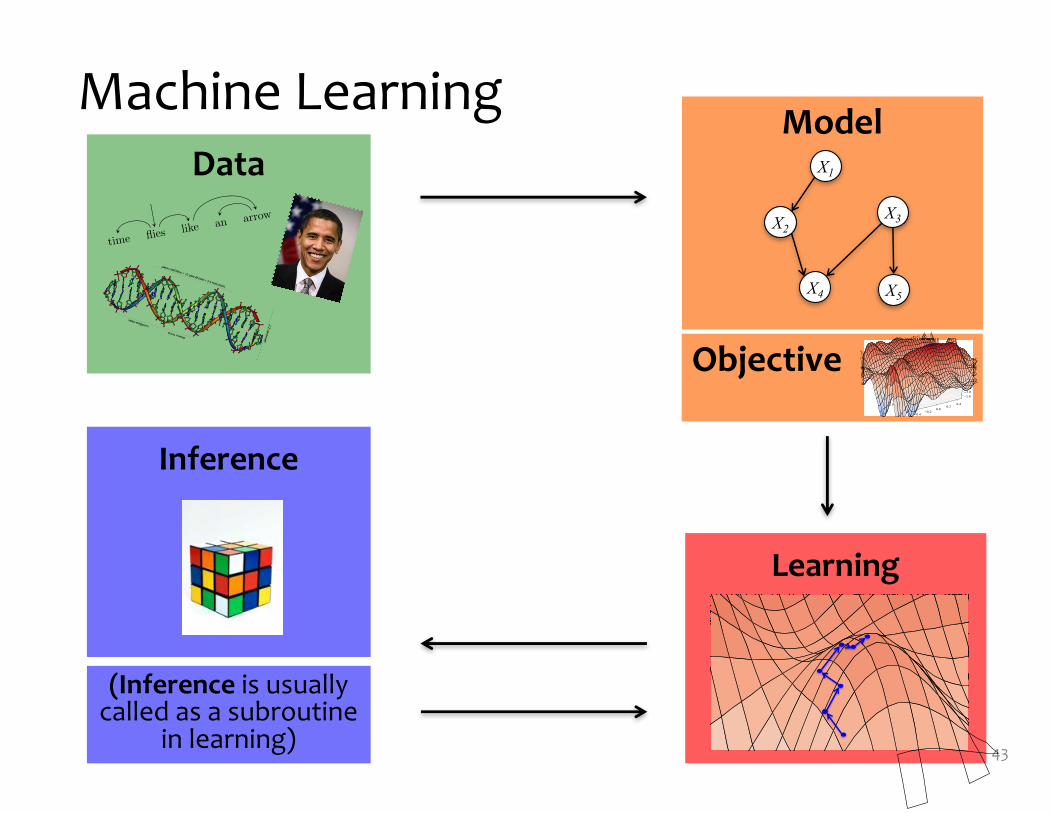
Machine Learning
43
DataModel
Learning
Inference
(Inference is usually called as a subroutine
in learning)
3
A
l
i
c
e
s
a
w
B
o
b
o
n
a
h
i
l
l
w
i
t
h
a
t
e
l
e
s
c
o
p
e
A
l
i
c
e
s
a
w
B
o
b
o
n
a
h
i
l
l
w
i
t
h
a
t
e
l
e
s
c
o
p
e
4
t
i
m
e
fl
i
e
s
l
i
k
e
a
n
a
r
r
o
w
t
i
m
e
fl
i
e
s
l
i
k
e
a
n
a
r
r
o
w
t
i
m
e
fl
i
e
s
l
i
k
e
a
n
a
r
r
o
w
t
i
m
e
fl
i
e
s
l
i
k
e
a
n
a
r
r
o
w
t
i
m
e
fl
i
e
s
l
i
k
e
a
n
a
r
r
o
w
2
Objective
X1
X3X2
X4 X5
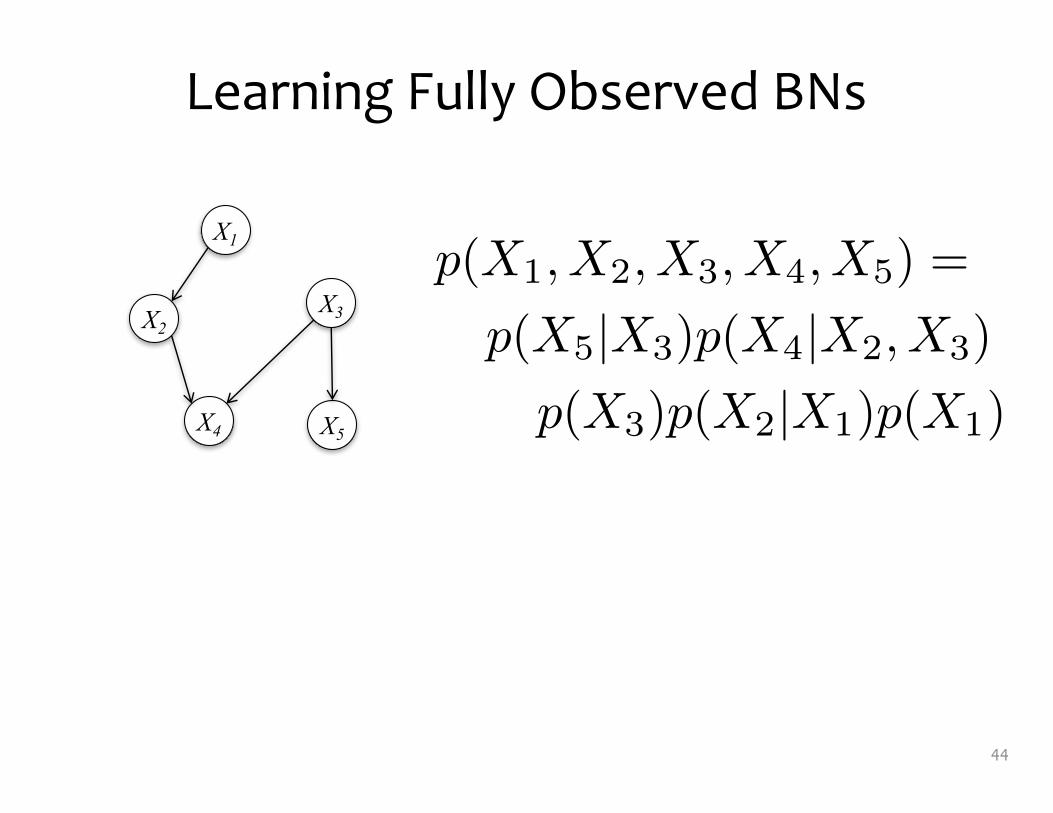
Learning Fully Observed BNs
44
X1
X3X2
X4 X5
p(X1, X2, X3, X4, X5) =
p(X5|X3)p(X4|X2, X3)
p(X3)p(X2|X1)p(X1)

p(X1, X2, X3, X4, X5) =
p(X5|X3)p(X4|X2, X3)
p(X3)p(X2|X1)p(X1)
Learning Fully Observed BNs
45
X1
X3X2
X4 X5
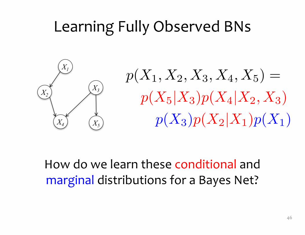
p(X1, X2, X3, X4, X5) =
p(X5|X3)p(X4|X2, X3)
p(X3)p(X2|X1)p(X1)
Learning Fully Observed BNs
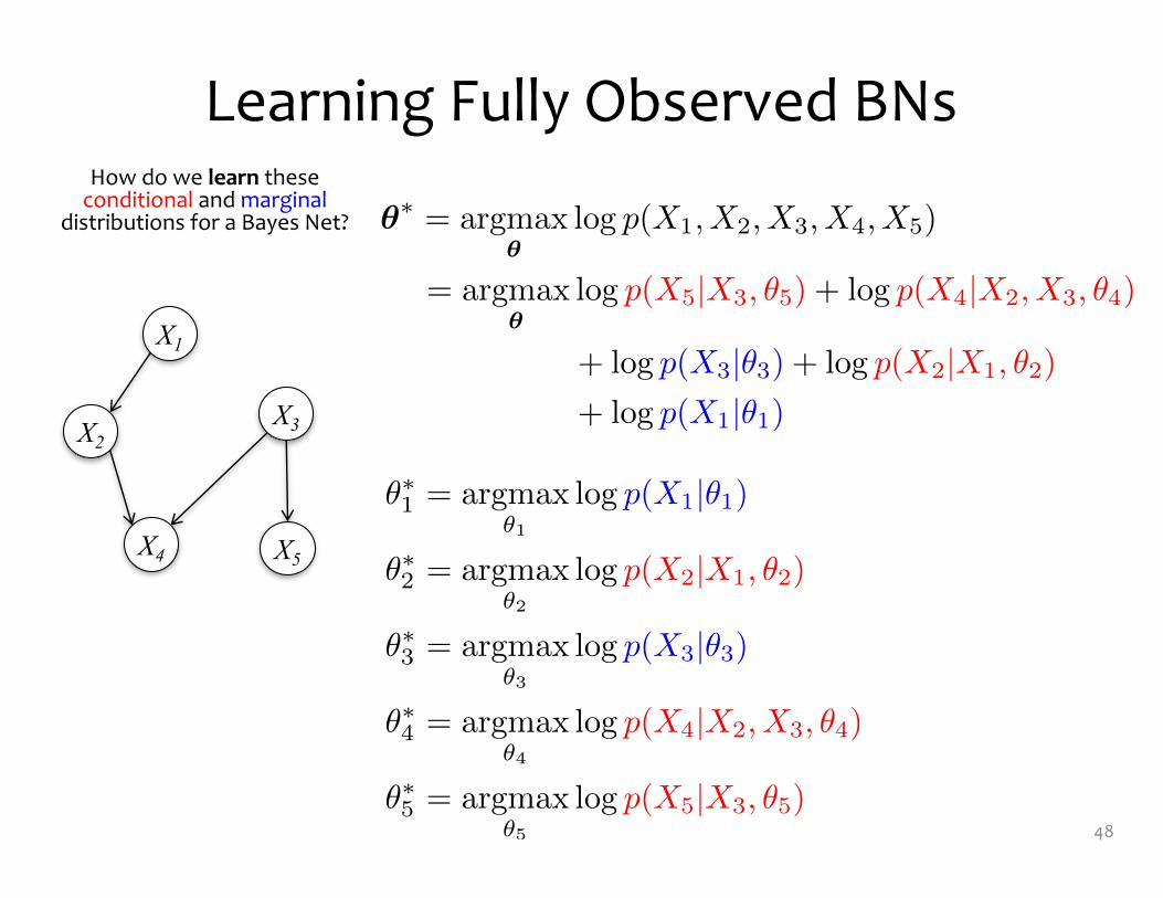
How do we learn these conditional and marginal distributions for a Bayes Net?
46
X1
X3X2
X4 X5

Learning Fully Observed BNs
47
X1
X3X2
X4 X5
p(X1, X2, X3, X4, X5) =
p(X5|X3)p(X4|X2, X3)
p(X3)p(X2|X1)p(X1)
X1
X2
X1
X3
X3X2
X4
X3
X5
Learning this fully observed Bayesian Network is equivalent to learning five (small / simple) independent networks from the same data
Learning Fully Observed BNs
48
X1
X3X2
X4 X5
✓⇤= argmax
✓log p(X1, X2, X3, X4, X5)
= argmax
✓log p(X5|X3, ✓5) + log p(X4|X2, X3, ✓4)
+ log p(X3|✓3) + log p(X2|X1, ✓2)
+ log p(X1|✓1)
✓⇤1 = argmax
✓1
log p(X1|✓1)
✓⇤2 = argmax
✓2
log p(X2|X1, ✓2)
✓⇤3 = argmax
✓3
log p(X3|✓3)
✓⇤4 = argmax
✓4
log p(X4|X2, X3, ✓4)
✓⇤5 = argmax
✓5
log p(X5|X3, ✓5)
✓⇤= argmax
✓log p(X1, X2, X3, X4, X5)
= argmax
✓log p(X5|X3, ✓5) + log p(X4|X2, X3, ✓4)
+ log p(X3|✓3) + log p(X2|X1, ✓2)
+ log p(X1|✓1)
How do we learn these conditional and marginal
distributions for a Bayes Net?

Learning Fully Observed BNs
Whiteboard– Example: Learning for Tornado Alarms
49

INFERENCE FOR BAYESIAN NETWORKS
52
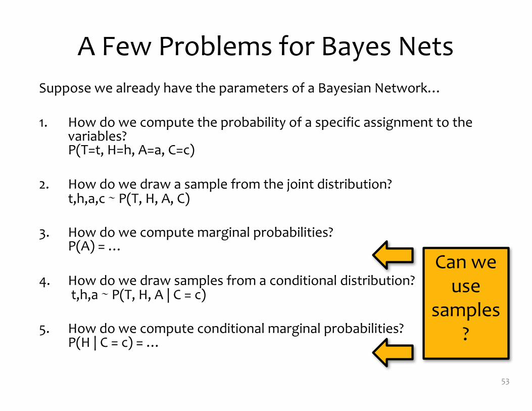
A Few Problems for Bayes NetsSuppose we already have the parameters of a Bayesian Network…
1. How do we compute the probability of a specific assignment to the variables?P(T=t, H=h, A=a, C=c)
2. How do we draw a sample from the joint distribution?t,h,a,c � P(T, H, A, C)
3. How do we compute marginal probabilities?P(A) = …
4. How do we draw samples from a conditional distribution? t,h,a � P(T, H, A | C = c)
5. How do we compute conditional marginal probabilities?P(H | C = c) = …
53
Can we use
samples?

Inference for Bayes Nets
Whiteboard– Background: Marginal Probability– Sampling from a joint distribution– Gibbs Sampling
54
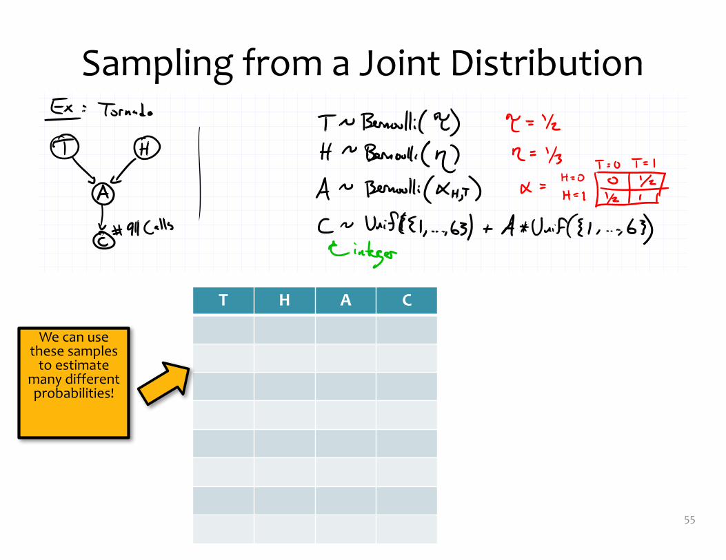
Sampling from a Joint Distribution
55
T H A C
We can use these samples
to estimate many different probabilities!

Gibbs Sampling
56
Copyright Cambridge University Press 2003. On-screen viewing permitted. Printing not permitted. http://www.cambridge.org/0521642981You can buy this book for 30 pounds or $50. See http://www.inference.phy.cam.ac.uk/mackay/itila/ for links.
370 29 — Monte Carlo Methods
(a)x1
x2
P (x)
(b)x1
x2
P (x1 |x(t)2 )
x(t)
(c)x1
x2
P (x2 |x1)
(d)x1
x2
x(t)
x(t+1)
x(t+2)
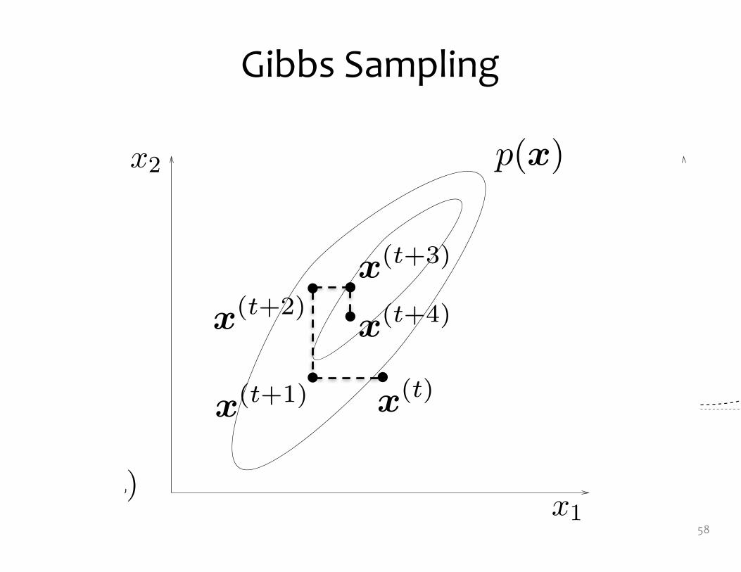
Figure 29.13. Gibbs sampling.(a) The joint density P (x) fromwhich samples are required. (b)Starting from a state x(t), x1 issampled from the conditionaldensity P (x1 |x(t)
2 ). (c) A sampleis then made from the conditionaldensity P (x2 |x1). (d) A couple ofiterations of Gibbs sampling.
This is good news and bad news. It is good news because, unlike thecases of rejection sampling and importance sampling, there is no catastrophicdependence on the dimensionality N . Our computer will give useful answersin a time shorter than the age of the universe. But it is bad news all the same,because this quadratic dependence on the lengthscale-ratio may still force usto make very lengthy simulations.
Fortunately, there are methods for suppressing random walks in MonteCarlo simulations, which we will discuss in the next chapter.
29.5 Gibbs sampling
We introduced importance sampling, rejection sampling and the Metropolismethod using one-dimensional examples. Gibbs sampling, also known as theheat bath method or ‘Glauber dynamics’, is a method for sampling from dis-tributions over at least two dimensions. Gibbs sampling can be viewed as aMetropolis method in which a sequence of proposal distributions Q are definedin terms of the conditional distributions of the joint distribution P (x). It isassumed that, whilst P (x) is too complex to draw samples from directly, itsconditional distributions P (xi | {xj}j =i) are tractable to work with. For manygraphical models (but not all) these one-dimensional conditional distributionsare straightforward to sample from. For example, if a Gaussian distributionfor some variables d has an unknown mean m, and the prior distribution of mis Gaussian, then the conditional distribution of m given d is also Gaussian.Conditional distributions that are not of standard form may still be sampledfrom by adaptive rejection sampling if the conditional distribution satisfiescertain convexity properties (Gilks and Wild, 1992).
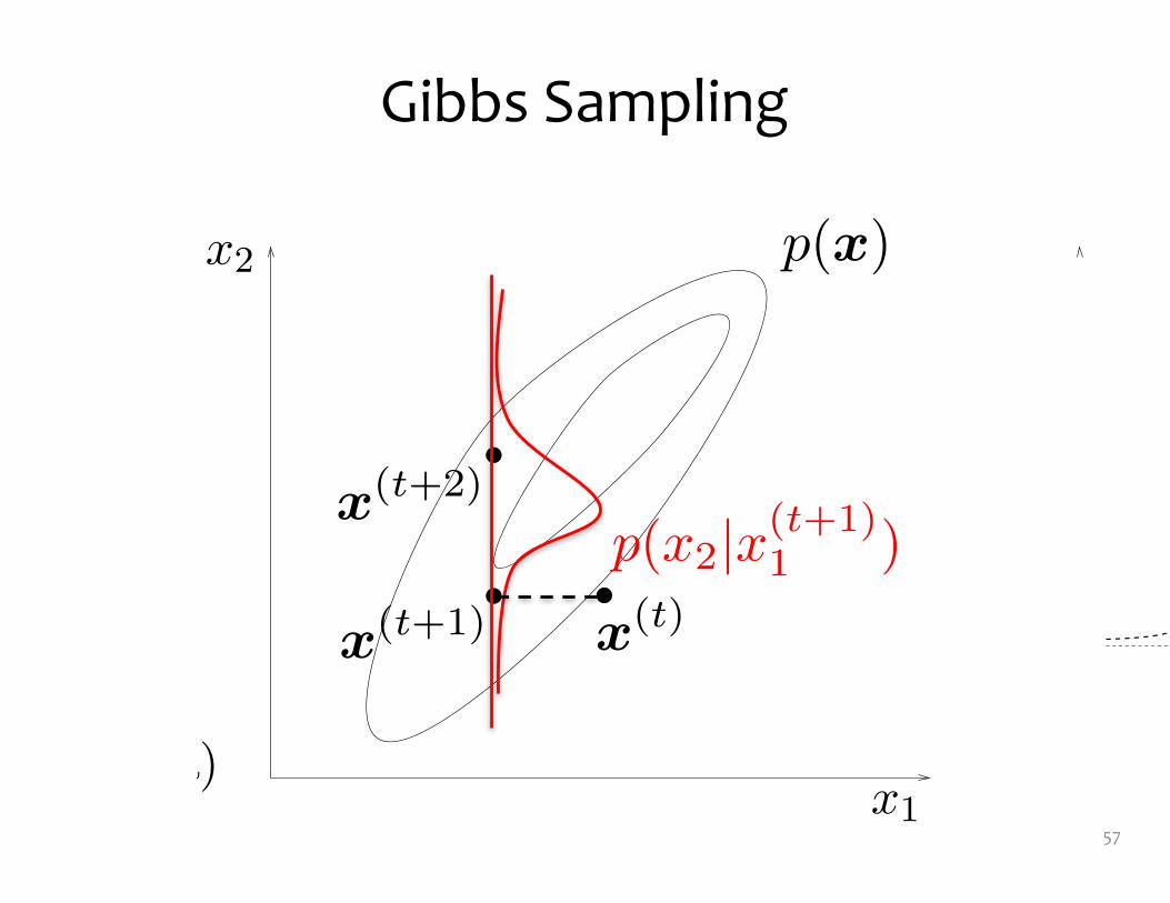
Gibbs sampling is illustrated for a case with two variables (x1, x2) = xin figure 29.13. On each iteration, we start from the current state x(t), andx1 is sampled from the conditional density P (x1 |x2), with x2 fixed to x(t)
2 .A sample x2 is then made from the conditional density P (x2 |x1), using the
p(x)
p(x1|x(t)2 )
x
(t)x
(t+1)
Gibbs Sampling
57
Copyright Cambridge University Press 2003. On-screen viewing permitted. Printing not permitted. http://www.cambridge.org/0521642981You can buy this book for 30 pounds or $50. See http://www.inference.phy.cam.ac.uk/mackay/itila/ for links.
370 29 — Monte Carlo Methods
(a)x1
x2
P (x)
(b)x1
x2
P (x1 |x(t)2 )
x(t)
(c)x1
x2
P (x2 |x1)
(d)x1
x2
x(t)
x(t+1)
x(t+2)
Figure 29.13. Gibbs sampling.(a) The joint density P (x) fromwhich samples are required. (b)Starting from a state x(t), x1 issampled from the conditionaldensity P (x1 |x(t)
2 ). (c) A sampleis then made from the conditionaldensity P (x2 |x1). (d) A couple ofiterations of Gibbs sampling.
This is good news and bad news. It is good news because, unlike thecases of rejection sampling and importance sampling, there is no catastrophicdependence on the dimensionality N . Our computer will give useful answersin a time shorter than the age of the universe. But it is bad news all the same,because this quadratic dependence on the lengthscale-ratio may still force usto make very lengthy simulations.
Fortunately, there are methods for suppressing random walks in MonteCarlo simulations, which we will discuss in the next chapter.
29.5 Gibbs sampling
We introduced importance sampling, rejection sampling and the Metropolismethod using one-dimensional examples. Gibbs sampling, also known as theheat bath method or ‘Glauber dynamics’, is a method for sampling from dis-tributions over at least two dimensions. Gibbs sampling can be viewed as aMetropolis method in which a sequence of proposal distributions Q are definedin terms of the conditional distributions of the joint distribution P (x). It isassumed that, whilst P (x) is too complex to draw samples from directly, itsconditional distributions P (xi | {xj}j =i) are tractable to work with. For manygraphical models (but not all) these one-dimensional conditional distributionsare straightforward to sample from. For example, if a Gaussian distributionfor some variables d has an unknown mean m, and the prior distribution of mis Gaussian, then the conditional distribution of m given d is also Gaussian.Conditional distributions that are not of standard form may still be sampledfrom by adaptive rejection sampling if the conditional distribution satisfiescertain convexity properties (Gilks and Wild, 1992).
Gibbs sampling is illustrated for a case with two variables (x1, x2) = xin figure 29.13. On each iteration, we start from the current state x(t), andx1 is sampled from the conditional density P (x1 |x2), with x2 fixed to x(t)
2 .A sample x2 is then made from the conditional density P (x2 |x1), using the
p(x)
x
(t+1)
x
(t+2)
p(x2|x(t+1)1 )
x
(t)
Gibbs Sampling
58
Copyright Cambridge University Press 2003. On-screen viewing permitted. Printing not permitted. http://www.cambridge.org/0521642981You can buy this book for 30 pounds or $50. See http://www.inference.phy.cam.ac.uk/mackay/itila/ for links.
370 29 — Monte Carlo Methods
(a)x1
x2
P (x)
(b)x1
x2
P (x1 |x(t)2 )
x(t)
(c)x1
x2
P (x2 |x1)
(d)x1
x2
x(t)
x(t+1)
x(t+2)
Figure 29.13. Gibbs sampling.(a) The joint density P (x) fromwhich samples are required. (b)Starting from a state x(t), x1 issampled from the conditionaldensity P (x1 |x(t)
2 ). (c) A sampleis then made from the conditionaldensity P (x2 |x1). (d) A couple ofiterations of Gibbs sampling.
This is good news and bad news. It is good news because, unlike thecases of rejection sampling and importance sampling, there is no catastrophicdependence on the dimensionality N . Our computer will give useful answersin a time shorter than the age of the universe. But it is bad news all the same,because this quadratic dependence on the lengthscale-ratio may still force usto make very lengthy simulations.
Fortunately, there are methods for suppressing random walks in MonteCarlo simulations, which we will discuss in the next chapter.
29.5 Gibbs sampling
We introduced importance sampling, rejection sampling and the Metropolismethod using one-dimensional examples. Gibbs sampling, also known as theheat bath method or ‘Glauber dynamics’, is a method for sampling from dis-tributions over at least two dimensions. Gibbs sampling can be viewed as aMetropolis method in which a sequence of proposal distributions Q are definedin terms of the conditional distributions of the joint distribution P (x). It isassumed that, whilst P (x) is too complex to draw samples from directly, itsconditional distributions P (xi | {xj}j =i) are tractable to work with. For manygraphical models (but not all) these one-dimensional conditional distributionsare straightforward to sample from. For example, if a Gaussian distributionfor some variables d has an unknown mean m, and the prior distribution of mis Gaussian, then the conditional distribution of m given d is also Gaussian.Conditional distributions that are not of standard form may still be sampledfrom by adaptive rejection sampling if the conditional distribution satisfiescertain convexity properties (Gilks and Wild, 1992).
Gibbs sampling is illustrated for a case with two variables (x1, x2) = xin figure 29.13. On each iteration, we start from the current state x(t), andx1 is sampled from the conditional density P (x1 |x2), with x2 fixed to x(t)
2 .A sample x2 is then made from the conditional density P (x2 |x1), using the
p(x)
x
(t+1)
x
(t+2)
x
(t)
x
(t+3)
x
(t+4)
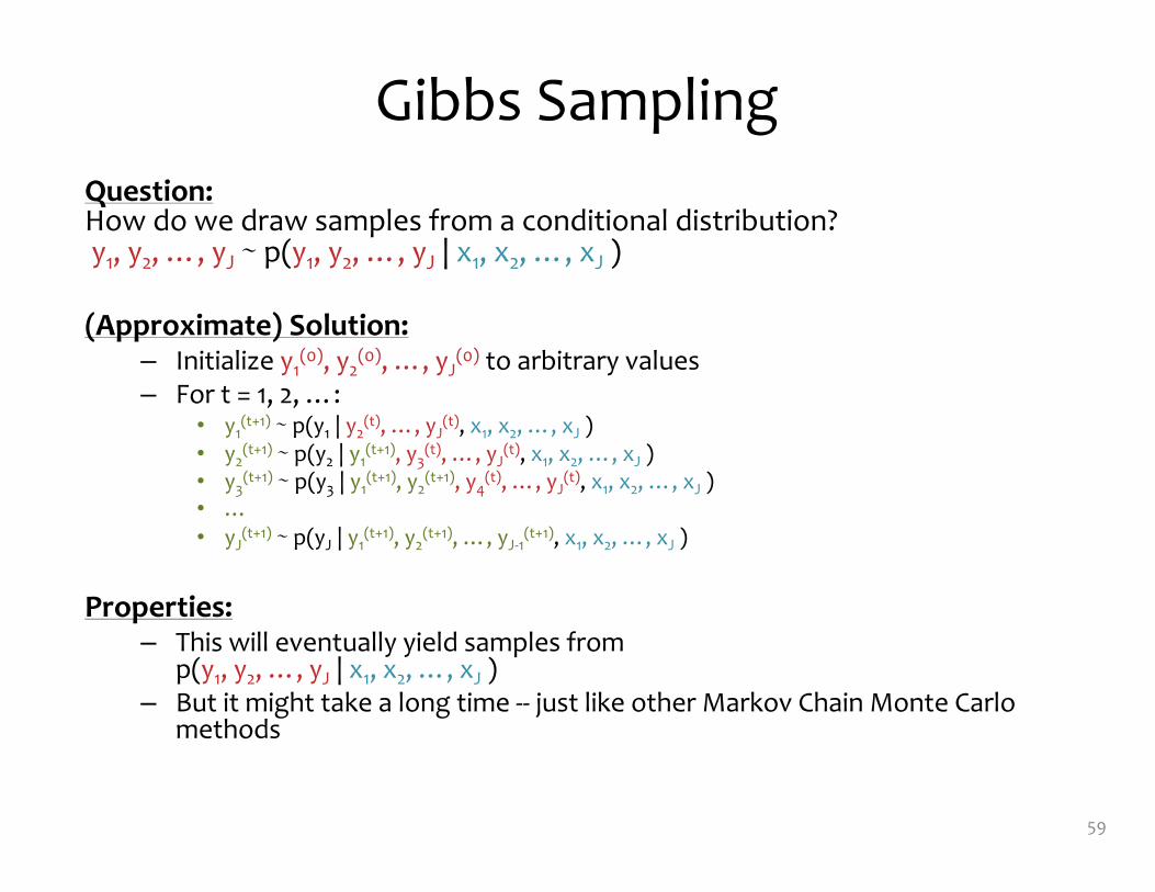
Gibbs SamplingQuestion:How do we draw samples from a conditional distribution? y1, y2, …, yJ � p(y1, y2, …, yJ | x1, x2, …, xJ )
(Approximate) Solution:– Initialize y1
(0), y2(0), …, yJ
(0) to arbitrary values– For t = 1, 2, …:
• y1(t+1) � p(y1 | y2
(t), …, yJ(t), x1, x2, …, xJ )
• y2(t+1) � p(y2 | y1
(t+1), y3(t), …, yJ
(t), x1, x2, …, xJ )• y3
(t+1) � p(y3 | y1(t+1), y2
(t+1), y4(t), …, yJ
(t), x1, x2, …, xJ )• …• yJ
(t+1) � p(yJ | y1(t+1), y2
(t+1), …, yJ-1(t+1), x1, x2, …, xJ )
Properties:– This will eventually yield samples from
p(y1, y2, …, yJ | x1, x2, …, xJ )– But it might take a long time -- just like other Markov Chain Monte Carlo
methods
59

Gibbs Sampling
Full conditionals only need to condition on the Markov Blanket
60
• Must be “easy” to sample from conditionals
• Many conditionals are log-concave and are amenable to adaptive rejection sampling
X1
X4X3
X6 X7
X9
X12
X5
X2
X8
X10
X13
X11

Learning ObjectivesBayesian Networks
You should be able to…1. Identify the conditional independence assumptions given by a generative
story or a specification of a joint distribution2. Draw a Bayesian network given a set of conditional independence
assumptions3. Define the joint distribution specified by a Bayesian network4. User domain knowledge to construct a (simple) Bayesian network for a real-
world modeling problem5. Depict familiar models as Bayesian networks6. Use d-separation to prove the existence of conditional indenpendencies in a
Bayesian network7. Employ a Markov blanket to identify conditional independence assumptions
of a graphical model8. Develop a supervised learning algorithm for a Bayesian network9. Use samples from a joint distribution to compute marginal probabilities10. Sample from the joint distribution specified by a generative story11. Implement a Gibbs sampler for a Bayesian network
61