Bayesian Multivariate Time Series Methods forEmpirical Macroeconomics�

Gary KoopUniversity of Strathclyde

Dimitris KorobilisUniversity of Strathclyde

April 2010

Abstract

Macroeconomic practitioners frequently work with multivariate timeseries models such as VARs, factor augmented VARs as well as time-varying parameter versions of these models (including variants with mul-tivariate stochastic volatility). These models have a large number of pa-rameters and, thus, over-parameterization problems may arise. Bayesianmethods have become increasingly popular as a way of overcoming theseproblems. In this monograph, we discuss VARs, factor augmented VARsand time-varying parameter extensions and show how Bayesian inferenceproceeds. Apart from the simplest of VARs, Bayesian inference requiresthe use of Markov chain Monte Carlo methods developed for state spacemodels and we describe these algorithms. The focus is on the empiri-cal macroeconomist and we o¤er advice on how to use these models andmethods in practice and include empirical illustrations. A website pro-vides Matlab code for carrying out Bayesian inference in these models.

1 Introduction

The purpose of this monograph is to o¤er a survey of the Bayesian methodsused with many of the models used in modern empirical macroeconomics. Thesemodels have been developed to address the fact that most questions of inter-est to empirical macroeconomists involve several variables and, thus, must beaddressed using multivariate time series methods. Many di¤erent multivariatetime series models have been used in macroeconomics, but since the pioneeringwork of Sims (1980), Vector Autoregressive (VAR) models have been amongthe most popular. It soon became apparent that, in many applications, theassumption that the VAR coe¢ cients were constant over time might be a poorone. For instance, in practice, it is often found that the macroeconomy of the

�Both authors are Fellows at the Rimini Centre for Economic Analysis. Address for corre-spondence: Gary Koop, Department of Economics, University of Strathclyde, 130 Rottenrow,Glasgow G4 0GE, UK. Email: Gary.Koop@strath.ac.uk

1

1960s and 1970s was di¤erent from the 1980s and 1990s. This led to an in-terest in models which allowed for time variation in the VAR coe¢ cients andtime-varying parameter VARs (TVP-VARs) arose. In addition, in the 1980smany industrialized economies experienced a reduction in the volatility of manymacroeconomic variables. This Great Moderation of the business cycle led toan increasing focus on appropriate modelling of the error covariance matrix inmultivariate time series models and this led to the incorporation of multivariatestochastic volatility in many empirical papers. In 2008 many economies wentinto recession and many of the associated policy discussions suggest that theparameters in VARs may be changing again.Macroeconomic data sets typically involve monthly, quarterly or annual ob-

servations and, thus are only of moderate size. But VARs have a great numberof parameters to estimate. This is particularly true if the number of dependentvariables is more than two or three (as is required for an appropriate mod-elling of many macroeconomic relationships). Allowing for time-variation inVAR coe¢ cients causes the number of parameters to proliferate. Allowing forthe error covariance matrix to change over time only increases worries aboutover-parameterization. The research challenge facing macroeconomists is howto build models that are �exible enough to be empirically relevant, capturingkey data features such as the Great Moderation, but not so �exible as to beseriously over-parameterized. Many approaches have been suggested, but acommon theme in most of these is shrinkage. Whether for forecasting or es-timation, it has been found that shrinkage can be of great bene�t in reducingover-parameterization problems. This shrinkage can take the form of imposingrestrictions on parameters or shrinking them towards zero. This has initiated alarge increase in the use of Bayesian methods since prior information provides alogical and formally consistent way of introducing shrinkage.1 Furthermore, thecomputational tools necessary to carry out Bayesian estimation of high dimen-sional multivariate time series models have become well-developed and, thus,models which may have been di¢ cult or impossible to estimate ten or twentyyears ago can now be routinely used by macroeconomic practitioners.A related class of models, and associated worries about over-parameterization,

has arisen due to the increase in data availability. Macroeconomists are able towork with hundreds of di¤erent time series variables collected by governmentstatistical agencies and other policy institutes. Building a model with hundredsof time series variables (with at most a few hundred observations on each) is adaunting task, raising the issue of a potential proliferation of parameters anda need for shrinkage or other methods for reducing the dimensionality of themodel. Factor methods, where the information in the hundreds of variablesis distilled into a few factors, are a popular way of dealing with this prob-lem. Combining factor methods with VARs results in Factor-augmented VARs

1Prior information can be purely subjective. However, as will be discussed below, oftenempirical Bayesian or hierarchical priors are used by macroeconomists. For instance, the stateequation in a state space model can be interpreted as a hierarchical prior. But, when we havelimited data information relative to the number of parameters, the role of the prior becomesincreasingly in�uential. In such cases, great care must to taken with prior elicitation.

2

or FAVARs. However, just as with VARs, there is a need to allow for time-variation in parameters, which leads to an interest in TVP-FAVARs. Here, too,Bayesian methods are popular and for the same reason as with TVP-VARs:Bayesian priors provide a sensible way of avoiding over-parameterization prob-lems and Bayesian computational tools are well-designed for dealing with suchmodels.In this monograph, we survey, discuss and extend the Bayesian literature on

VARs, TVP-VARs and TVP-FAVARs with a focus on the practitioner. Thatis, we go beyond simply de�ning each model, but specify how to use them inpractice, discuss the advantages and disadvantages of each and o¤er some tipson when and why each model can be used. In addition to this, we discuss somenew modelling approaches for TVP-VARs. A website contains Matlab codewhich allows for Bayesian estimation of the models discussed in this monograph.Bayesian inference often involves the use of Markov chain Monte Carlo (MCMC)posterior simulation methods such as the Gibbs sampler. For many of themodels, we provide complete details in this monograph. However, in some caseswe only provide an outline of the MCMC algorithm. Complete details of allalgorithms are given in a manual on the website.Empirical macroeconomics is a very wide �eld and VARs, TVP-VARs and

factor models, although important, are only some of the tools used in the �eld.It is worthwhile brie�y mentioning what we are not covering in this monograph.There is virtually nothing in this monograph about macroeconomic theory andhow it might infuse econometric modelling. For instance, Bayesian estima-tion of dynamic stochastic general equilibrium (DSGE) models is very popular.There will be no discussion of DSGE models in this monograph (see An andSchorfheide, 2007 or Del Negro and Schorfheide, 2010 for excellent treatmentsof Bayesian DSGE methods with Chib and Ramamurthy, 2010 providing a re-cent important advance in computation). Also, macroeconomic theory is oftenused to provide identifying restrictions to turn reduced form VARs into struc-tural VARs suitable for policy analysis. We will not discuss structural VARs,although some of our empirical examples will provide impulse responses fromstructural VARs using standard identifying assumptions.There is also a large literature on what might, in general, be called regime-

switching models. Examples include Markov switching VARs, threshold VARs,smooth transition VARs, �oor and ceiling VARs, etc. These, although impor-tant, are not discussed here.The remainder of this monograph is organized as follows. Section 2 provides

discussion of VARs to develop some basic insights into the sorts of shrinkagepriors (e.g. the Minnesota prior) and methods of �nding empirically-sensiblerestrictions (e.g. stochastic search variable selection, or SSVS) that are usedin empirical macroeconomics. Our goal is to extend these basic methods andpriors used with VARs, to TVP variants. However, before considering theseextensions, Section 3 discusses Bayesian inference in state space models usingMCMC methods. We do this since TVP-VARs (including variants with multi-variate stochastic volatility) are state space models and it is important that thepractitioner knows the Bayesian tools associated with state space models before

3

proceeding to TVP-VARs. Section 4 discusses Bayesian inference in TVP-VARs,including variants which combine the Minnesota prior or SSVS with the stan-dard TVP-VAR. Section 5 discusses factor methods, beginning with the dynamicfactor model, before proceeding to the factor augmented VAR (FAVAR) andTVP-FAVAR. Empirical illustrations are used throughout and Matlab code forimplementing these illustrations (or, more generally, doing Bayesian inferencein VARs, TVP-VARs and TVP-FAVARs) is available on the website associatedwith this monograph.2

2 Bayesian VARs

2.1 Introduction and Notation

The VAR(p) model can be written as:

yt = a0 +

pXj=1

Ajyt�j + "t (1)

where yt for t = 1; ::; T is an M � 1 vector containing observations on M timeseries variables, "t is anM�1 vector of errors, a0 is anM�1 vector of interceptsand Aj is an M �M matrix of coe¢ cients. We assume "t to be i.i.d. N (0;�).Exogenous variables or more deterministic terms (e.g. deterministic trends orseasonals) can easily be added to the VAR and included in all the derivationsbelow, but we do not do so to keep the notation as simple as possible.The VAR can be written in matrix form in di¤erent ways and, depending on

how this is done, some of the literature expresses results in terms of the mul-tivariate Normal and others in terms of the matric-variate Normal distribution(see, e.g. Canova, 2007, and Kadiyala and Karlsson, 1997). The former arises ifwe use anMT�1 vector y which stacks all T observations on the �rst dependentvariable, then all T observations on the second dependent variable, etc.. Thelatter arises if we de�ne Y to be a T�M matrix which stacks the T observationson each dependent variable in columns next to one another. " and E denotestackings of the errors in a manner conformable to y and Y , respectively. De�next =

�1; y0t�1; ::; y

0t�p�and

X =

26664x1x2...xT

37775 : (2)

Note that, if we let K = 1+Mp be the number of coe¢ cients in each equationof the VAR, then X is a T �K matrix.Finally, if A = (a0 A1 :: Ap)

0 we de�ne � = vec (A) which is a KM � 1vector which stacks all the VAR coe¢ cients (and the intercepts) into a vector.With all these de�nitions, we can write the VAR either as:

2The website address is: http://personal.strath.ac.uk/gary.koop/bayes_matlab_code_by_koop_and_korobilis.html

4

Y = XA+ E (3)

or

y = (IM X)�+ "; (4)

where " � N (0;� IT ).The likelihood function can be derived from the sampling density, p (yj�;�).

If it is viewed as a function of the parameters, then it can be shown to be of aform that breaks into two parts: one a distribution for � given � and anotherwhere ��1 has a Wishart distribution.3 That is,

�j�; y � N�b�;� (X 0X)

�1�

(5)

and��1jy �W

�S�1; T �K �M � 1

�; (6)

where bA = (X 0X)�1X 0Y is the OLS estimate of A and b� = vec� bA� and

S =�Y �X bA�0 �Y �X bA� :

2.2 Priors

A variety of priors can be used with the VAR, of which we discuss some usefulones below. They di¤er in relation to three issues.First, VARs are not parsimonious models. They have a great many coe¢ -

cients. For instance, � contains KM parameters which, for a VAR(4) involving5 dependent variables is 105. With quarterly macroeconomic data, the numberof observations on each variable might be at most a few hundred. Without priorinformation, it is hard to obtain precise estimates of so many coe¢ cients and,thus, features such as impulse responses and forecasts will tend to be impre-cisely estimated (i.e. posterior or predictive standard deviations can be large).For this reason, it can be desirable to �shrink�forecasts and prior informationo¤ers a sensible way of doing this shrinkage. The priors discussed below di¤erin the way they achieve this goal.Second, the priors used with VARs di¤er in whether they lead to analytical

results for the posterior and predictive densities or whether MCMC methodsare required to carry out Bayesian inference. With the VAR, natural conju-gate priors lead to analytical results, which can greatly reduce the computa-tional burden. Particularly if one is carrying out a recursive forecasting exercisewhich requires repeated calculation of posterior and predictive distributions,non-conjugate priors which require MCMC methods can be very computation-ally demanding.

3 In this monograph, we use standard notational conventions to de�ne all distributions suchas the Wishart. See, among many other places, the appendix to Koop, Poirier and Tobias(2007). Wikipedia is also a quick and easy source of information about distributions.

5

Third, the priors di¤er in how easily they can handle departures from theunrestricted VAR given in (1) such as allowing for di¤erent equations to havedi¤erent explanatory variables, allowing for VAR coe¢ cients to change overtime, allowing for heteroskedastic structures for the errors of various sorts, etc.Natural conjugate priors typically do not lend themselves to such extensions.

2.2.1 The Minnesota Prior

Early work with Bayesian VARs with shrinkage priors was done by researchersat the University of Minnesota or the Federal Reserve Bank of Minneapolis (seeDoan, Litterman and Sims, 1984 and Litterman, 1986). The priors they usedhave come to be known as Minnesota priors. They are based on an approxima-tion which leads to great simpli�cations in prior elicitation and computation.This approximation involves replacing � with an estimate, b�. The original Min-nesota prior simpli�es even further by assuming � to be a diagonal matrix. Inthis case, each equation of the VAR can be estimated one at a time and wecan set b�ii = s2i (where s2i is the standard OLS estimate of the error variancein the ith equation and b�ii is the iith element of b�). When � is not assumedto be diagonal, a simple estimate such as b� = S

T can be used. A disadvantageof this approach is that it involves replacing an unknown matrix of parametersby an estimate (and potentially a poor one) rather than integrating it out ina Bayesian fashion. The latter strategy will lead to predictive densities whichmore accurately re�ect parameter uncertainty. However, as we shall see below,replacing � by an estimate simpli�es computation since analytical posterior andpredictive results are available. And it allows for a great range of �exibility inthe choice of prior. If � is not replaced by an estimate, the only fully Bayesianapproach which leads to analytical results involves the use of a natural conju-gate prior. As we shall see, the natural conjugate prior has some restrictiveproperties that may be unattractive in some cases.When � is replaced by an estimate, we only have to worry about a prior for

� and the Minnesota prior assumes:

� � N (�Mn; VMn) : (7)

The Minnesota prior can be thought of as a way of automatically choosing �Mn

and VMn in a manner which is sensible in many empirical contexts. To explainthe Minnesota prior, note �rst that the explanatory variables in the VAR in anyequation can be divided into the own lags of the dependent variable, the lagsof the other dependent variables and exogenous or deterministic variables (inequation 1 the intercept is the only exogenous or deterministic variable, but ingeneral there can be more such variables).For the prior mean, �Mn, the Minnesota prior involves setting most or all

of its elements to zero (thus ensuring shrinkage of the VAR coe¢ cients towardszero and lessening the risk of over-�tting). When using growth rates data (e.g.GDP growth, the growth in the money supply, etc., which are typically found tobe stationary and exhibit little persistence), it is sensible to simply set �Mn =

6

0KM . However, when using levels data (e.g. GDP, the money supply, etc.)the Minnesota prior uses a prior mean expressing a belief that the individualvariables exhibit random walk behavior. Thus, �Mn = 0KM except for theelements corresponding to the �rst own lag of the dependent variable in eachequation. These elements are set to one. These are the traditional choices for�Mn, but anything is possible. For instance, in our empirical illustration we setthe prior mean for the coe¢ cient on the �rst own lag to be 0:9, re�ecting a priorbelief that our variables exhibit a fair degree of persistence, but not unit rootbehavior.The Minnesota prior assumes the prior covariance matrix, VMn, to be diag-

onal. If we let V i denote the block of VMn associated with the K coe¢ cients inequation i and V i;jj be its diagonal elements, then a common implementationof the Minnesota prior would set:

V i;jj =

8<:a1r2 for coe¢ cients on own lag r for r = 1; ::; pa2�iir2�jj

for coe¢ cients on lag r of variable j 6= i for r = 1; ::; pa3�ii for coe¢ cients on exogenous variables

: (8)

This prior simpli�es the complicated choice of fully specifying all the ele-ments of VMn to choosing three scalars, a1; a2; a3. This form captures the sen-sible properties that, as lag length increases, coe¢ cients are increasingly shrunktowards zero and that (by setting a1 > a2) own lags are more likely to be im-portant predictors than lags of other variables. The exact choice of values fora1; a2; a3 depends on the empirical application at hand and the researcher maywish to experiment with di¤erent values for them. Typically, the researcher sets�ii = s

2i . Litterman (1986) provides much additional motivation and discussion

of these choices (e.g. an explanation for how the term �ii�jj

adjusts for di¤erencesin the units that the variables are measured in).Many variants of the Minnesota prior have been used in practice (e.g. Kadiyala

and Karlsson, 1997, divide prior variances by r instead of the r2 which is usedin (8)) as researchers make slight adjustments to tailor the prior for their partic-ular application. The Minnesota prior has enjoyed a recent boom in popularitybecause of its simplicity and success in many applications, particularly involvingforecasting. For instance, Banbura, Giannone and Reichlin (2010) use a slightmodi�cation of the Minnesota prior in a large VAR with over 100 dependentvariables. Typically, factor methods are used with such large panels of data,but Banbura, Giannone and Reichlin (2010) �nd that the Minnesota prior leadsto even better forecasting performance than factor methods.A big advantage of the Minnesota prior is that it leads to simple poste-

rior inference involving only the Normal distribution. It can be show that theposterior for � has the form:

�jy � N��Mn; VMn

�(9)

where

7

VMn =hV �1Mn +

�b��1 (X 0X)�i�1

and

�Mn = VMn

�V �1Mn�Mn +

�b��1 X�0 y� :But, as stressed above, a disadvantage of the Minnesota prior is that it does

not provide a full Bayesian treatment of � as an unknown parameter. Insteadit simply plugs in � = b�, ignoring any uncertainty in this parameter. In theremainder of this section we will discuss methods which treat � as an unknownparameter. However, as we shall see, this means (apart from one restrictivespecial case) that analytical methods are not available and MCMC methods arerequired).

2.2.2 Natural conjugate priors

Natural conjugate priors are those where the prior, likelihood and posteriorcome from the same family of distributions. Our previous discussion of thelikelihood function (see equations 5 and 6) suggests that, for the VAR, thenatural conjugate prior has the form:

�j� � N (�;� V ) (10)

and��1 �W

�S�1; �

�(11)

where �; V ; � and S are prior hyperparameters chosen by the researcher.With this prior the posterior becomes:

�j�; y � N��;� V

�(12)

and��1jy �W

�S�1; ��

(13)

where

V =�V �1 +X 0X

��1;

A = VhV �1A+X 0X bAi ;

� = vec�A�,

S = S + S + bA0X 0X bA+A0V �1A�A0 �V �1 +X 0X�A

and

� = T + �:

8

In the previous formulae, we use notation where A is a K �M matrix made byunstacking the KM � 1 vector �.Posterior inference about the VAR coe¢ cients can be carried out using the

fact that the marginal posterior (i.e. after integrating out �) for � is a multivari-ate t-distribution. The mean of this t-distribution is �, its degrees of freedomparameter is � and its covariance matrix is:

var (�jy) = 1

� �M � 1S V :

These facts can be used to carry out posterior inference in this model.The predictive distribution for yT+1 in this model has an analytical form

and, in particular, is multivariate-t with � degrees of freedom. The predictivemean of yT+1 is

�xT+1A

�0which can be used to produce point forecasts. The

predictive covariance matrix is 1��2

�1 + xT+1V x

0T+1

�S. When forecasting more

than one period ahead, an analytical formula for the predictive density does notexist. This means that either the direct forecasting method must be used (whichturns the problem into one which only involves one step ahead forecasting) orpredictive simulation is required.Any values for the prior hyperparameters, �; V ; � and S, can be chosen.

The noninformative prior is obtained by setting � = S = V �1 = cI and lettingc ! 0. It can be seen that this leads to posterior and predictive results whichare based on familiar OLS quantities. The drawback of the noninformative prioris that it does not do any of the shrinkage which we have argued is so importantfor VAR modelling.Thus, for the natural conjugate prior, analytical results exist which allow for

Bayesian estimation and prediction. There is no need to use posterior simula-tion algorithms unless interest centers on nonlinear functions of the parameters(e.g. impulse response analysis such as those which arise in structural VARs,see Koop, 1992). The posterior distribution of, e.g., impulse responses can beobtained by Monte Carlo integration. That is, draws of ��1 can be obtainedfrom (13) and, conditional on these, draws of � can be taken from (12).4 Thendraws of impulse responses can be calculated using these drawn values of ��1

and �.However, there are two properties of this prior that can be undesirable in

some circumstances. The �rst is that the (IM X) form of the explanatoryvariables in (4) means that every equation must have the same set of explanatoryvariables. For an unrestricted VAR this is �ne, but is not appropriate if theresearcher wishes to impose restrictions. Suppose, for instance, the researcher isworking with a VAR involving variables such as output growth and the growth inthe money supply and wants to impose a strict form of the neutrality of money.This would imply that the coe¢ cients on the lagged money growth variables inthe output growth equation are zero (but coe¢ cients of lagged money growth in

4Alternatively, draws of � can be directly taken from its multivariate-t marginal posteriordistribution.

9

other equations would not be zero). Such restrictions cannot be imposed withthe natural conjugate prior described here.To explain the second possibly undesirable property of this prior, we intro-

duce notation where individual elements of � are denoted by �ij . The fact thatthe prior covariance matrix has the form �V (which is necessary to ensure nat-ural conjugacy of the prior), implies that the prior covariance of the coe¢ cientsin equation i is �iiV . This means that the prior covariance of the coe¢ cients inany two equations must be proportional to one another, a possibly restrictivefeature. In our example, the researcher believing in the neutrality of moneymay wish to proceed as follows: in the output growth equation, the prior meanof the coe¢ cients on lagged money growth variables should be zero and theprior covariance matrix should be very small (i.e. expressing a prior belief thatthese coe¢ cients are very close to zero). In other equations, the prior covariancematrix on the coe¢ cients on lagged money growth should be much larger. Thenatural conjugate prior does not allow us to use prior information of this form.It also does not allow us to use the Minnesota prior. That is, the Minnesotaprior covariance matrix in (8) is written in terms of blocks which were labelledV i;jj involving i subscripts. That is, these blocks vary across equations whichis not allowed for in the natural conjugate prior.These two properties should be kept in mind when using the natural conju-

gate prior. There are generalizations of this natural conjugate prior, such as theextended natural conjugate prior of Kadiyala and Karlsson (1997), which sur-mount these problems. However, these lose the huge advantage of the naturalconjugate prior described in this section: that analytical results are availableand so no posterior simulation is required.A property of natural conjugate priors is that, since the prior and likelihood

have the same distributional form, the prior can be considered as arising froma �ctitious sample. For instance, a comparison of (5) and (10) shows that b�and (X 0X)

�1 in the likelihood play the same role as � and V in the prior. Thelatter can be interpreted as arising from a �ctitious sample (also called �dummyobservations�), Y0 and X0 (e.g. V = (X 0

0X0)�1 and � based on an OLS estimate

(X 00X0)

�1X 00Y0). This interpretation is developed in papers such as Sims (1993)

and Sims and Zha (1998). On one level, this insight can simply serve as anotherway of motivating choices for � and V as arising from particular choices forY0 and X0. But papers such as Sims and Zha (1998) show how the dummyobservation approach can be used to elicit priors for structural VARs. In thismonograph, we will focus on the econometric as opposed to the macroeconomicissues. Accordingly, we will work with reduced form VARs and not say muchabout structural VARs. Here we only note that posterior inference in structuralVARs is usually based on a reduced form VAR such as that discussed here, butthen coe¢ cients are transformed so as to give them a structural interpretation(see, e.g., Koop, 1992, for a simple example). For instance, structural VARs areoften written as:

10

C0yt = c0 +

pXj=1

Cjyt�j + ut (14)

where ut is i.i.d. N (0; I). Often appropriate identifying restrictions will providea one-to-one mapping from the parameters of the reduced form VAR in (1) to thestructural VAR. In this case, Bayesian inference can be done by using posteriorsimulation methods in the reduced form VAR and transforming each draw into adraw from the structural VAR. In models where such a one-to-one mapping doesnot exist (e.g. over-identi�ed structural VARs) alternative methods of posteriorinference exist (see Rubio-Ramirez, Waggoner and Zha, 2010).While discussing such macroeconomic issues, it is worth noting that there

is a growing literature that uses the insights of economic theory (e.g. from realbusiness cycle or DSGE models) to elicit priors for VARs. Prominent examplesinclude Ingram and Whiteman (1994) and Del Negro and Schorfheide (2004).We will not discuss this work in this monograph.Finally, it is also worth mentioning the work of Villani (2009) on steady state

priors for VARs. We have motivated prior information as being important as away of ensuring shrinkage in an over-parameterized VAR. However, most of theshrinkage discussed previously relates to the VAR coe¢ cients. Often researchershave strong prior information about the unconditional means (i.e. the steadystates) of the variables in their VARs. It is desirable to include such informationas an additional source of shrinkage in the VAR. However, it is not easy to dothis in the VAR in (1) since the intercepts cannot be directly interpreted as theunconditional means of the variables in the VAR. Villani (2009) recommendswriting the VAR as: eA (L) (yt � ea0) = "t (15)

where eA (L) = I� eA1L� ::� eApLp, L is the lag operator and "t is i.i.d. N (0;�).In this parameterization, ea0 can be interpreted as the vector of unconditionalmeans of the dependent variables and a prior placed on it re�ecting the re-searcher�s beliefs about steady state values for them. For eA (L) and � one ofthe priors described previously (or below) can be used. A drawback of thisapproach is that an analytical form for the posterior no longer exists. However,Villani (2009) develops a Gibbs sampling algorithm for carrying out Bayesianinference in this model.

2.2.3 The Independent Normal-Wishart Prior

The natural conjugate prior has the large advantage that analytical results areavailable for posterior inference and prediction. However, it does have the draw-backs noted previously (i.e. it assumes each equation to have the same explana-tory variables and it restricts the prior covariance of the coe¢ cients in any twoequations to be proportional to one another). Accordingly, in this section, weintroduce a more general framework for VAR modelling. Bayesian inferencein these models will require posterior simulation algorithms such as the Gibbssampler. The natural conjugate prior had �j� being Normal and ��1 being

11

Wishart. Note that the fact that the prior for � depends on � implies that �and � are not independent of one another. In this section, we work with a priorwhich has VAR coe¢ cients and the error covariance being independent of oneanother (hence the name �independent Normal-Wishart prior�).To allow for di¤erent equations in the VAR to have di¤erent explanatory

variables, we have to modify our previous notation slightly. To avoid any pos-sibility of confusion, we will use ��� as notation for VAR coe¢ cients in thisrestricted VAR model instead of �. We write each equation of the VAR as:

ymt = z0mt�m + "mt;

with t = 1; ::; T observations form = 1; ::;M variables. ymt is the tth observationon the mth variable, zmt is a km-vector containing the tth observation of thevector of explanatory variables relevant for the mth variable and �m is theaccompanying km-vector of regression coe¢ cients. Note that if we had zmt =�1; y0t�1; ::; y

0t�p�0for m = 1; ::;M then we would obtain the unrestricted VAR

of the previous section. However, by allowing for zmt to vary across equationswe are allowing for the possibility of a restricted VAR (i.e. it allows for some ofthe coe¢ cients on the lagged dependent variables to be restricted to zero).We can stack all equations into vectors/matrices as yt = (y1t; ::; yMt)

0, "t =("1t; ::; "Mt)

0,

� =

0B@ �1...�M

1CA ;

Zt =

0BBBB@z01t 0 � � � 0

0 z02t. . .

......

. . .. . . 0

0 � � � 0 z0Mt

1CCCCA ;where � is a k � 1 vector and Zt is M � k where k =

PMj=1 kj . As before, we

assume "t to be i.i.d. N (0;�).Using this notation, we can write the (possibly restricted) VAR as:

yt = Zt� + "t. (16)

Stacking as:

y =

0B@ y1...yT

1CA ;

" =

0B@ "1..."T

1CA ;12

Z =

0B@ Z1...ZT

1CAwe can write

y = Z� + "

and " is N (0; I �).It can be seen that the restricted VAR can be written as a Normal linear

regression model with an error covariance matrix of a particular form. A verygeneral prior for this model (which does not involve the restrictions inherent inthe natural conjugate prior) is the independent Normal-Wishart prior:

p��;��1

�= p (�) p

���1

�where

� � N��; V �

�(17)

and

��1 �W�S�1; �

�: (18)

Note that this prior allows for the prior covariance matrix, V � , to be anythingthe researcher chooses, rather than the restrictive � V form of the naturalconjugate prior. For instance, the researcher could set � and V � exactly asin the Minnesota prior. A noninformative prior can be obtained by setting� = S = V �1� = 0.Using this prior, the joint posterior p

��;��1jy

�does not have a conve-

nient form that would allow easy Bayesian analysis (e.g. posterior means andvariances do not have analytical forms). However, the conditional posteriordistributions p

��jy;��1

�and p

���1jy; �

�do have convenient forms:

�jy;��1 � N��; V �

�; (19)

where

V � =

V �1� +

TXt=1

Z 0t��1Zt

!�1and

� = V �

V �1� � +

TXi=1

Z 0t��1yt

!:

Furthermore,

13

��1jy; � �W�S�1; �;�

(20)

where

� = T + �

and

S = S +TXt=1

(yt � Zt�) (yt � Zt�)0 :

Accordingly, a Gibbs sampler which sequentially draws from the Normal p (�jy;�)and the Wishart p

���1jy; �

�can be programmed up in a straightforward fash-

ion. As with any Gibbs sampler, the resulting posterior simulator output canbe used to calculate posterior properties of any function of the parameters,marginal likelihoods (for model comparison) and/or to do prediction.Note that, for the VAR, Z� will contain lags of variables and, thus, contain

information dated � � 1 or earlier. The one-step ahead predictive density (i.e.the one for predicting at time � given information through � � 1), conditionalon the parameters of the model is:

y� jZ� ; �;� � N (Zt�;�) :

This result, along with a Gibbs sampler producing draws �(r);�(r) for r = 1; ::; Rallows for predictive inference.5 For instance, the predictive mean (a popularpoint forecast) could be obtained as:

E (y� jZ� ) =PR

r=1 Zt�(r)

R

and other predictive moments can be calculated in a similar fashion. Alterna-tively, predictive simulation can be done at each Gibbs sampler draw, but thiscan be computationally demanding. For forecast horizons greater than one, thedirect method can be used. This strategy for doing predictive analysis can beused with any of the priors or models discussed below.

2.2.4 Stochastic Search Variable Selection (SSVS) in VARs

SSVS as Implemented in George, Sun and Ni (2008) In the previoussections, we have described various priors for unrestricted and restricted VARswhich allow for shrinkage of VAR coe¢ cients. However, these approaches re-quired substantial prior input from the researcher (although this prior input canbe of an automatic form such as in the Minnesota prior). There is another priorthat, in a sense, does shrinkage and leads to restricted VARs, but does so in anautomatic fashion that requires only minimal prior input from the researcher.

5Typically, some initial draws are discarded as the �burn in�. Accordingly, r = 1; ::; Rshould be the post-burn in draws.

14

The methods associated with this prior are called SSVS and are enjoying in-creasing popularity and, accordingly, we describe them here in detail. SSVS canbe done in several ways. Here we describe the implementation of George, Sunand Ni (2008).The basic idea underlying SSVS can be explained quite simply. Suppose �j

is a VAR coe¢ cient. Instead of simply using a prior for it as before (e.g. asin (10), SSVS speci�es a hierarchical prior (i.e. a prior expressed in terms ofparameters which in turn have a prior of their own) which is a mixture of twoNormal distributions:

�j j j ��1� j

�N�0; �20j

�+ jN

�0; �21j

�; (21)

where j is a dummy variable. If j equals one then �j is drawn from the secondNormal and if it equals zero then �j is drawn from the �rst Normal. The prioris hierarchical since j is treated as an unknown parameter and estimated in adata-based fashion. The SSVS aspect of this prior arises by choosing the �rstprior variance, �20j , to be �small� (so that the coe¢ cient is constrained to bevirtually zero) and the second prior variance, �21j , to be �large�(implying a rela-tively noninformative prior for the corresponding coe¢ cient). Below we describewhat George, Sun and Ni (2008) call a �default semi-automatic approach� tochoosing �20j and �

21j which requires minimal subjective prior information from

the researcher.The SSVS approach can be thought of as automatically selecting a restricted

VAR since it can, in a data-based fashion, set j = 0 and (to all intents andpurposes) delete the corresponding lagged dependent variable form the model.Alternatively, SSVS can be thought of as a way of doing shrinkage since VARcoe¢ cients can be shrunk to zero.The researcher can also carry out a Bayesian unrestricted VAR analysis using

an SSVS prior, then use the output from this analysis to select a restricted VAR(which can then be estimated using, e.g., a noninformative or an independentNormal-Wishart prior). This can be done by using the posterior p ( jY ) where = ( 1; ::; KM )

0. One common strategy is to use b , the mode of p ( jY ). Thiswill be a vector of zeros and ones and the researcher can simply omit explanatoryvariables corresponding to the zeros. The relationship between such a strategyand conventional model selection techniques using an information criteria (e.g.the Akaike or Bayesian information criteria) is discussed in Fernandez, Ley andSteel (2001). Alternatively, if the MCMC algorithm described below is simplyrun and posterior results for the VAR coe¢ cients calculated using the resultingMCMC output, the result will be Bayesian model averaging (BMA).In this section, we focus on SSVS, but it is worth mentioning that there are

many other Bayesian methods for selecting a restricted model or doing BMA.In cases where the number of models under consideration is small, it is possibleto simply calculate the marginal likelihoods for every model and use these asweights when doing BMA or simply to select the single model with the highestmarginal likelihood. Marginal likelihoods for the multivariate time series modelsdiscussed in this monograph can be calculated in several ways (see Section 3).

15

In cases (such as the present ones) where the number of restricted models isvery large, various other approaches have been suggested, see Green (1995) andCarlin and Chib (1995). See also Chipman, George and McCulloch (2001) for asurvey on Bayesian model selection and, in particular, the discussion of practicalissues is prior elicitation and posterior simulation that arise.SSVS allows us to work with the unrestricted VAR and have the algorithm

pick out an appropriate restricted VAR. Accordingly we will return to our no-tation for the unrestricted VAR (see Section 2.1). The unrestricted VAR iswritten in (3) and � is the KM � 1 vector of VAR coe¢ cients. SSVS can beinterpreted as de�ning a hierarchical prior for all of the elements of � and �.The prior for � given in (21) can be written more compactly as:

�j � N (0; DD) ; (22)

where D is a diagonal matrix with (j; j)th element given by dj where

dj =

��0j if j = 0�1j if j = 1

: (23)

Note that this prior implies a mixture of two Normals as written in (21).George, Sun and Ni (2008) describe a �default semi-automatic approach�to

selecting the prior hyperparameters �0j and �1j which involves setting �0j =c0pdvar(�j) and �1j = c1pdvar(�j) wheredvar(�j) is an estimate of the variance

of the coe¢ cient in an unrestricted VAR (e.g. the ordinary least squares quantityor an estimate based on a preliminary Bayesian estimation the VAR using anoninformative prior). The pre-selected constants c0 and c1 must have c0 � c1(e.g. c0 = 0:1 and c1 = 10).For = ( 1; ::; KM )

0, the SSVS prior assumes that each element has aBernoulli form (independent of the other elements of ) and, hence, for j =1; ::;KM , we have

Pr� j = 1

�= q

j

Pr� j = 0

�= 1� q

j

: (24)

A natural default choice is qj= 0:5 for all j, implying each coe¢ cient is a priori

equally likely to be included as excluded.So far, we have said nothing about the prior for � and (for the sake of

brevity) we will not provide details relating to it. Su¢ ce it to note here that if aWishart prior for ��1 like (18) is used, then a formula very similar to (20) canbe used as a block in a Gibbs sampling algorithm. Alternatively, George, Sunand Ni (2008) use a prior for � which allows for them to do SSVS on the errorcovariance matrix. That is, although they always assume the diagonal elementsof � are positive (so as to ensure a positive de�nite error covariance matrix),they allow for parameters which determine the o¤-diagonal elements to havean SSVS prior thus allowing for restrictions to be imposed on �. We refer theinterested reader to George, Sun and Ni (2008) or the manual on the websiteassociated with this monograph for details.

16

Posterior computation in the VAR with SSVS prior can be carried out usinga Gibbs sampling algorithm. For the VAR coe¢ cients we have

�jy; ;� � N(��; V �); (25)

where

V � = [��1 (X 0X) + (DD)

�1]�1;

�� = V �[(0) (X 0X)�];

A = (X 0X)�1X 0Y

and

� = vec(A):

The conditional posterior for has j being independent Bernoulli randomvariables:

Pr� j = 1jy; �

�= qj ;

Pr� j = 0jy; �

�= 1� qj ;

(26)

where

qj =

1

�1jexp

��2j2�21j

!qj

1

�1jexp

��2j2�21j

!qj+

1

�0jexp

��2j2�20j

!�1� q

j

� :Thus, a Gibbs sampler involving the Normal distribution and the Bernoulli

distribution (and either the Gamma or Wishart distributions depending on whatprior is used for ��1) allows for posterior inference in this model.

SSVS as Implemented in Korobilis (2009b) The implementation of SSVSjust described is a popular one. However, there are other similar methods forautomatic model selection in VARs. In particular, the approach of George, Sunand Ni (2008) involves selecting values for the �small�prior variance �0j . Thereader may ask why not set �small�exactly equal to zero? This has been done inregression models in papers such as Kuo and Mallick (1997) through restrictingcoe¢ cients to be precisely zero if j = 0. There are some subtle statisticalissues which arise when doing this.6 Korobilis (2009b) has extended the use ofsuch methods to VARs. Since, unlike the implementation of George, Sun and

6For instance, asympotically such priors will always set j = 1 for all j.

17

Ni (2008), this approach leads to restricted VARs (as opposed to unrestrictedVARs with very tight priors on some of the VAR coe¢ cients), we return to ournotation for restricted VARs and modify it slightly. In particular, replace (16)by

yt = Zte� + "t. (27)

where e� = eD� and eD is a diagonal matrix with the jth diagonal element being j (where, as before, j is a dummy variable). In words, this model allows foreach VAR coe¢ cient to be set to zero (if j = 0) or included in an unrestrictedfashion (if j = 1).Bayesian inference using the prior can be carried out in a straightforward

fashion. For exact details on the necessary MCMC algorithm, see Korobilis(2009b) and the manual on the website associated with this book. However, theidea underlying this algorithm can be explained quite simply. Conditional on , this model is a restricted VAR and the MCMC algorithm of Section 2.2.2 forthe independent Normal-Wishart prior can be used. Thus, all that is required isa method for taking draws from (conditional on the parameters of the VAR).Korobilis (2009b) derives the necessary distribution.

2.3 Empirical Illustration of Bayesian VAR Methods

To illustrate Bayesian VAR methods using some of the priors and methods de-scribed above, we use a quarterly US data set on the in�ation rate ��t (theannual percentage change in a chain-weighted GDP price index), the unemploy-ment rate ut (seasonally adjusted civilian unemployment rate, all workers overage 16) and the interest rate rt (yield on the three month Treasury bill rate).Thus yt = (��t; ut; rt)

0. The sample runs from 1953Q1 to 2006Q3. Thesethree variables are commonly used in New Keynesian VARs.7 Examples of pa-pers which use these, or similar, variables include Cogley and Sargent (2005),Primiceri (2005) and Koop, Leon-Gonzalez and Strachan (2009). The data areplotted in Figure 1.

7The data are obtained from the Federal Reserve Bank of St. Louis website,http://research.stlouisfed.org/fred2/.

18

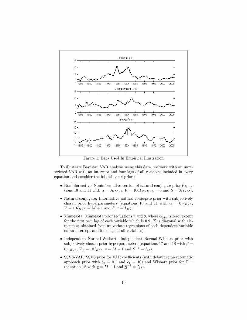
Figure 1: Data Used In Empirical Illustration

To illustrate Bayesian VAR analysis using this data, we work with an unre-stricted VAR with an intercept and four lags of all variables included in everyequation and consider the following six priors:

� Noninformative: Noninformative version of natural conjugate prior (equa-tions 10 and 11 with � = 0KM�1, V = 100IK�K , v = 0 and S = 0M�M ).

� Natural conjugate: Informative natural conjugate prior with subjectivelychosen prior hyperparameters (equations 10 and 11 with � = 0KM�1,V = 10IK , v =M + 1 and S�1 = IM ).

� Minnesota: Minnesota prior (equations 7 and 8, where �Mn is zero, exceptfor the �rst own lag of each variable which is 0:9. � is diagonal with ele-ments s2i obtained from univariate regressions of each dependent variableon an intercept and four lags of all variables).

� Independent Normal-Wishart: Independent Normal-Wishart prior withsubjectively chosen prior hyperparameters (equations 17 and 18 with � =0KM�1, V � = 10IKM , v =M + 1 and S�1 = IM ).

� SSVS-VAR: SSVS prior for VAR coe¢ cients (with default semi-automaticapproach prior with c0 = 0:1 and c1 = 10) and Wishart prior for ��1

(equation 18 with v =M + 1 and S�1 = IM ).

19

� SSVS: SSVS on both VAR coe¢ cients and error covariance (default semi-automatic approach).8

For the �rst three priors, analytical posterior and predictive results are avail-able. For the last three, posterior and predictive simulation is required. Theresults below are based on 50000 MCMC draws, for which the �rst 20000 arediscarded as burn-in draws. For impulse responses (which are nonlinear func-tions of the VAR coe¢ cients and �), posterior simulation methods are requiredfor all six priors.With regards to impulse responses, they are identi�ed by assuming C0 in

(14) is lower triangular and the dependent variables are ordered as: in�ation,unemployment and interest rate. This is a standard identifying assumption used,among many others, by Bernanke and Mihov (1998), Christiano, Eichanbaumand Evans (1999) and Primiceri (2005). It allows for the interpretation of theinterest rate shock as a monetary policy shock.With VARs, the parameters themselves (as opposed to functions of them

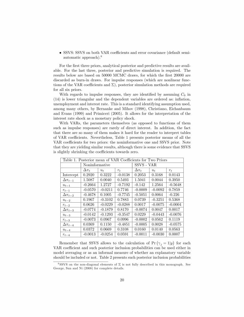
such as impulse responses) are rarely of direct interest. In addition, the factthat there are so many of them makes it hard for the reader to interpret tablesof VAR coe¢ cients. Nevertheless, Table 1 presents posterior means of all theVAR coe¢ cients for two priors: the noninformative one and SSVS prior. Notethat they are yielding similar results, although there is some evidence that SSVSis slightly shrinking the coe¢ cients towards zero.

Table 1. Posterior mean of VAR Coe¢ cients for Two PriorsNoninformative SSVS - VAR��t ut rt ��t ut rt

Intercept 0.2920 0.3222 -0.0138 0.2053 0.3168 0.0143��t�1 1.5087 0.0040 0.5493 1.5041 0.0044 0.3950ut�1 -0.2664 1.2727 -0.7192 -0.142 1.2564 -0.5648rt�1 -0.0570 -0.0211 0.7746 -0.0009 -0.0092 0.7859��t�2 -0.4678 0.1005 -0.7745 -0.5051 0.0064 -0.226ut�2 0.1967 -0.3102 0.7883 0.0739 -0.3251 0.5368rt�2 0.0626 -0.0229 -0.0288 0.0017 -0.0075 -0.0004��t�3 -0.0774 -0.1879 0.8170 -0.0074 0.0047 0.0017ut�3 -0.0142 -0.1293 -0.3547 0.0229 -0.0443 -0.0076rt�3 -0.0073 0.0967 0.0996 -0.0002 0.0562 0.1119��t�4 0.0369 0.1150 -0.4851 -0.0005 0.0028 -0.0575ut�4 0.0372 0.0669 0.3108 0.0160 0.0140 0.0563rt�4 -0.0013 -0.0254 0.0591 -0.0011 -0.0030 0.0007

Remember that SSVS allows to the calculation of Pr� j = 1jy

�for each

VAR coe¢ cient and such posterior inclusion probabilities can be used either inmodel averaging or as an informal measure of whether an explanatory variableshould be included or not. Table 2 presents such posterior inclusion probabilities

8SSVS on the non-diagonal elements of � is not fully described in this monograph. SeeGeorge, Sun and Ni (2008) for complete details.

20

using the SSVS-VAR prior. The empirical researcher may wish to present sucha table for various reasons. For instance, if the researcher wishes to select asingle restricted VAR which only includes coe¢ cients with Pr

� j = 1jy

�> 1

2 ,then he would work with a model which restricts 25 of 39 coe¢ cients to zero.Table 2 shows which coe¢ cients are important. Of the 14 included coe¢ cientstwo are intercepts and three are �rst own lags in each equation. The researcherusing SSVS to select a single model would restrict most of the remaining VARcoe¢ cients to be zero. The researcher using SSVS to do model averaging would,in e¤ect, be restricting them to be approximately zero. Note also that SSVScan be used to do lag length selection in an automatic fashion. None of thecoe¢ cients on the fourth lag variables is found to be important and only one ofnine possible coe¢ cients on third lags is found to be important.

Table 2. Posterior Inclusion Probabilities forVAR Coe¢ cients: SSVS-VAR Prior

��t ut rtIntercept 0.7262 0.9674 0.1029��t�1 1 0.0651 0.9532ut�1 0.7928 1 0.8746rt�1 0.0612 0.2392 1��t�2 0.9936 0.0344 0.5129ut�2 0.4288 0.9049 0.7808rt�2 0.0580 0.2061 0.1038��t�3 0.0806 0.0296 0.1284ut�3 0.2230 0.2159 0.1024rt�3 0.0416 0.8586 0.6619��t�4 0.0645 0.0507 0.2783ut�4 0.2125 0.1412 0.2370rt�4 0.0556 0.1724 0.1097

With VARs, the researcher is often interested in forecasting. It is worthmentioning that often recursive forecasting exercises, which involve forecastingat time � = �0; ::; T , are often done. These typically involve estimating a modelT � �0 times using appropriate sub-samples of the data. If MCMC methodsare required, this can be computationally demanding. That is, running anMCMC algorithm T � �0 times can (depending on the model and application)be very slow. If this is the case, then the researcher may be tempted to workwith methods which do not require MCMC such as the Minnesota or naturalconjugate priors. Alternatively, sequential importance sampling methods suchas the particle �lter (see, e.g. Doucet, Godsill and Andrieu, 2000 or Johannesand Polson, 2009) can be used which do not require the MCMC algorithm tobe run at each point in time.9

Table 3 presents predictive results for an out-of-sample forecasting exercisebased on the predictive density p (yT+1jy1::; yT ) where T = 2006Q3. It can be

9Although the use of particle �ltering raises empirical challenges of its own which we willnot discuss here.

21

seen that for this empirical example, which involves a moderately large dataset, the prior is having relatively little impact. That is, predictive means andstandard deviations are similar for all six priors, although it can be seen that thepredictive standard deviations with the Minnesota prior do tend to be slightlysmaller than the other priors.

Table 3. Predictive mean of yT+1 (st. dev. in parentheses)PRIOR ��T+1 uT+1 rT+1

Noninformative3.105(0.315)

4.610(0.318)

4.382(0.776)

Minnesota3.124(0.302)

4.628(0.319)

4.350(0.741)

Natural conjugate3.106(0.313)

4.611(0.314)

4.380(0.748)

Indep. Normal-Wishart3.110(0.322)

4.622(0.324)

4.315(0.780)

SSVS - VAR3.097(0.323)

4.641(0.323)

4.281(0.787)

SSVS3.108(0.304)

4.639(0.317)

4.278(0.785)

True value, yT+1 3.275 4.700 4.600

Figures 2 and 3 present impulse responses of all three of our variables to allthree of the shocks for two of the priors: the noninformative one and the SSVSprior. In these �gures the posterior median is the solid line and the dotted linesare the 10th and 90th percentiles. These impulse responses all have sensibleshapes, similar to those found by other authors. The two priors are givingsimilar results, but a careful examination of them do reveal some di¤erences.Especially at longer horizons, there is evidence that SSVS leads to slightly moreprecise inferences (evidenced by a narrower band between the 10th and 90th

percentiles) due to the shrinkage it provides.

22

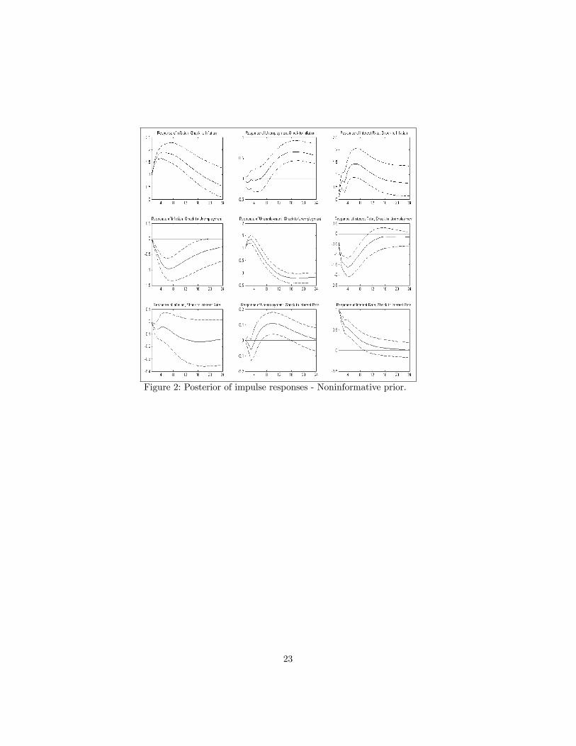
Figure 2: Posterior of impulse responses - Noninformative prior.

23

Figure 3: Posterior of impulse responses - SSVS prior.

2.4 Empirical Illustration: Forecasting with VARs

Our previous empirical illustration used a small VAR and focussed largely onimpulse response analysis. However, VARs are commonly used for forecastingand, recently, there has been a growing interest in larger Bayesian VARs. Hence,we provide a forecasting application with a larger VAR.Banbura, Giannone and Reichlin (2010) work with VARs with up to 130

dependent variables and �nd that they forecast well relative to popular alterna-tives such as factor models (a class of models which is discussed below). Theyuse a Minnesota prior. Koop (2010) carries out a similar forecasting exercise,with a wider range of priors and wider range of VARs of di¤erent dimensions.Note that a 20-variate VAR(4) with quarterly data would have M = 20 andp = 4 in which case � contains over 1500 coe¢ cients. �, too, will be parameterrich, containing over 200 distinct elements. A typical macroeconomic quarterlydata set might have approximately two hundred observations and, hence, thenumber of coe¢ cients will far exceed the number of observations. But Bayesianmethods combine likelihood function with prior. It is well-known that, even ifsome parameters are not identi�ed in the likelihood function, under weak con-ditions the use of a proper prior will lead to a valid posterior density and, thus,

24

Bayesian inference is possible. However, prior information becomes increasinglyimportant as the number of parameters increases relative to sample size.The present empirical illustration uses the same US quarterly data set as

Koop (2010).10 The data runs from 1959Q1 through 2008Q4. We considersmall VARs with three dependent variables (M = 3) and larger VARs whichcontain the same three dependent variables plus 17 more (M = 20). All ourVARs have four lags. For brevity, we do not provide a precise list of variablesor data de�nitions (see Koop, 2010, for complete details). Here we note onlythe three main variables used with both VARs are the ones we are interestedin forecasting. These are a measure of economic activity (GDP, real GDP),prices (CPI, the consumer price index) and an interest rate (FFR, the Fedfunds rate). The remaining 17 variables used with the larger VAR are othercommon macroeconomic variables which are thought to potentially be of someuse for forecasting the main three variables.Following Stock and Watson (2008) and many others, the variables are all

transformed to stationarity (usually by di¤erencing or log di¤erencing). Withdata transformed in this way, we set the prior means for all coe¢ cients in allapproaches to zero (instead of setting some prior means to one so as to shrinktowards a random walk as might be appropriate if we were working with untrans-formed variables). We consider three priors: a Minnesota prior as implementedby Banbura, Giannone and Reichlin (2010), an SSVS prior as implemented inGeorge, Sun and Ni (2008) as well as a prior which combines the Minnesotaprior with the SSVS prior. This �nal prior is identical to the SSVS prior withone exception. To explain the one exception, remember that the SSVS priorinvolves setting the diagonal elements of the prior covariance matrix in (22)to be �0j = c0

pdvar(�j) and �1j = c1pdvar(�j) where dvar(�j) is based on a

posterior or OLS estimate. In our �nal prior, we set dvar(�j) to be the priorvariance of �j from the Minnesota prior. Other details of implementation (e.g.the remaining prior hyperparameter choices not speci�ed here) are as in Koop(2010). Su¢ ce it to note here that they are the same as those used in Banbura,Giannone and Reichlin (2010) and George, Sun and Ni (2008).Previously we have shown how to obtain predictive densities using these

priors. We also need a way of evaluating forecast performance. Here we considertwo measures of forecast performance: one is based on point forecasts, the otherinvolves entire predictive densities.We carry out a recursive forecasting exercise using the direct method. That

is, for � = �0; ::; T � h, we obtain the predictive density of y�+h using dataavailable through time � for h = 1 and 4. �0 is 1969Q4. In this forecastingsection, we will use notation where yi;�+h is a random variable we are wishingto forecast (e.g. GDP, CPI or FFR), yoi:�+h is the observed value of yi;�+h andp (yi;�+hjData� ) is the predictive density based on information available at time� .Mean square forecast error, MSFE, is the most common measure of forecast

10This is an updated version of the data set used in Stock and Watson (2008). We wouldlike to thank Mark Watson for making this data available.

25

comparison. It is de�ned as:

MSFE =

PT�h�=�0

hyoi;�+h � E (yi;�+hjData� )

i2T � h� �0 + 1

:

In Table 4, MSFE is presented as a proportion of the MSFE produced by randomwalk forecasts.MSFE only uses the point forecasts and ignores the rest of the predictive

distribution. Predictive likelihoods evaluate the forecasting performance of theentire predictive density. Predictive likelihoods are motivated and described inmany places such as Geweke and Amisano (2010). The predictive likelihood isthe predictive density for yi;�+h evaluated at the actual outcome yoi;�+h. Thesum of log predictive likelihoods can be used for forecast evaluation:

T�hX�=�0

log�p�yi;�+h = y

oi;�+hjData�

��:

Table 4 presents MSFEs and sums of log predictive likelihoods for our threemain variables of interest for forecast horizons one quarter and one year in thefuture. All of the Bayesian VARs forecast substantially better than a randomwalk for all variables. However, beyond that it is hard to draw any generalconclusion from Table 4. Each prior does well for some variable and/or fore-cast horizon. However, it is often the case that the prior which combines SSVSfeatures with Minnesota prior features forecasts best. Note that in the largerVAR the SSVS prior can occasionally perform poorly. This is because coe¢ -cients which are included (i.e. have j = 1) are not shrunk to any appreciabledegree. This lack of shrinkage can sometimes lead to a worsening of forecastperformance. By combining the Minnesota prior with the SSVS prior we cansurmount this problem.It can also be seen that usually (but not always), the larger VARs forecast

better than the small VAR. If we look only at the small VARs, the SSVS prioroften leads to the best forecast performance.Our two forecast metrics, MSFEs and sums of log predictive likelihoods,

generally point towards the same conclusion. But there are exceptions wheresums of log predictive likelihoods (the preferred Bayesian forecast metric) canpaint a di¤erent picture than MSFEs.

26

Table 4: MSFEs as Proportion of Random walk MSFEsSums of log predictive likelihoods in parenthesesVariable Minnesota Prior SSVS Prior SSVS+Minnesota

M = 3 M = 20 M = 3 M = 20 M = 3 M = 20Forecast Horizon of One Quarter

GDP0:650(�206:4)

0:552(�192:3)

0:606(�198:40)

0:641(�205:1)

0:698(�204:7)

0:647(�203:9)

CPI0:347(�201:2)

0:303(�195:9)

0:320(�193:9)

0:316(�196:5)

0:325(�191:5)

0:291(�187:6)

FFR0:619(�238:4)

0:514(�229:1)

0:844(�252:4)

0:579(�237:2)

0:744(�252:7)

0:543(�228:9)

Forecast Horizon of One Year

GDP0:744(�220:6)

0:609(�214:7)

0:615(�207:8)

0:754(�293:2)

0:844(�221:6)

0:667(�219:0)

CPI0:525(�209:5)

0:522(�219:4)

0:501(�208:3)

0:772(�276:4)

0:468(�194:4)

0:489(�201:6)

FFR0:668(�243:3)

0:587(�249:6)

0:527(�231:2)

0:881(�268:1)

0:618(�228:8)

0:518(�233:7)

3 Bayesian State Space Modeling and Stochas-tic Volatility

3.1 Introduction and Notation

In the section on Bayesian VAR modeling, we showed that the (possibly re-stricted) VAR could be written as:

yt = Zt� + "

for appropriate de�nitions of Zt and �. In many macroeconomic applications,it is undesirable to assume � to be constant, but it is sensible to assume that �evolves gradually over time. A standard version of the TVP-VAR which will bediscussed in the next section extends the VAR to:

yt = Zt�t + "t,

where

�t+1 = �t + ut:

Thus, the VAR coe¢ cients are allowed to vary gradually over time. This is astate space model.Furthermore, previously we assumed "t to be i.i.d. N (0;�) and, thus, the

model was homoskedastic. In empirical macroeconomics, it is often importantto allow for the error covariance matrix to change over time (e.g. due to theGreat Moderation of the business cycle) and, in such cases, it is desirable to

27

assume "t to be i.i.d. N (0;�t) so as to allow for heteroskedasticity. This raisesthe issue of stochastic volatility which, as we shall see, also leads us into theworld of state space models.These considerations provide a motivation for why we must provide a section

on state space models before proceeding to TVP-VARs and other models of moredirect relevance for empirical macroeconomics. We begin this section by �rstdiscussing Bayesian methods for the Normal linear state space model. Thesemethods can be used to model evolution of the VAR coe¢ cients in the TVP-VAR. Unfortunately, stochastic volatility cannot be written in the form of aNormal linear state space model. Thus, after brie�y discussing nonlinear statespace modelling in general, we present Bayesian methods for particular nonlinearstate space models of interest involving stochastic volatility.We will adopt a notational convention commonly used in the state space

literature where, if at is a time t quantity (i.e. a vector of states or data)then at = (a01; ::; a

0t)0 stacks all the ats up to time t. So, for instance, yT will

denote the entire sample of data on the dependent variables and �T the vectorcontaining all the states.

3.2 The Normal Linear State Space Model

A general formulation for the Normal linear state space model (which containsthe TVP-VAR de�ned above as a special case) is:

yt =Wt� + Zt�t + "t; (28)

and

�t+1 = �t�t + ut, (29)

where yt is an M � 1 vector containing observations on M time series variables,"t is an M � 1 vector of errors, Wt is a known M � p0 matrix (e.g. thiscould contain lagged dependent variables or other explanatory variables withconstant coe¢ cients), � is a p0 � 1 vector of parameters. Zt is a known M � kmatrix (e.g. this could contain lagged dependent variables or other explanatoryvariables with time varying coe¢ cients), �t is a k�1 vector of parameters whichevolve over time (these are known as states). We assume "t to be independentN (0;�t) and ut to be a k � 1 vector which is independent N (0; Qt). "t andus are independent of one another for all s and t. �t is a k � k matrix whichis typically treated as known, but occasionally �t is treated as a matrix ofunknown parameters.Equations (28) and (29) de�ne a state space model. Equation (28) is called

the measurement equation and (29) the state equation. Models such as thishave been used for a wide variety of purposes in econometrics and many other�elds. The interested reader is referred to West and Harrison (1997) and Kimand Nelson (1999) for a broader Bayesian treatment of state space models thanthat provided here. Harvey (1989) and Durbin and Koopman (2001) providegood non-Bayesian treatments of state space models.

28

For our purpose, the important thing to note is that, for given values of �, �t,�t and Qt (for t = 1; ::; T ), various algorithms have been developed which allowfor posterior simulation of �t for t = 1; ::; T . Popular and e¢ cient algorithms aredescribed in Carter and Kohn (1994), Fruhwirth-Schnatter (1994), DeJong andShephard (1995) and Durbin and Koopman (2002).11 Since these are standardand well-understood algorithms, we will not present complete details here. Inthe Matlab code on the website associated with this monograph, the algorithmof Carter and Kohn (1994) is used. These algorithms can be used as a blockin an MCMC algorithm to provide draws from the posterior of �t conditionalon �, �t, �t and Qt (for t = 1; ::; T ). The exact treatment of �, �t, �t andQt depends on the empirical application at hand. The standard TVP-VAR�xes some of these to known values (e.g. � = 0;�t = I are common choices)and treats others as unknown parameters (although it usually restricts Qt = Qand, in the case of the homoskedastic TVP-VAR additionally restricts �t = �for all t). An MCMC algorithm is completed by taking draws of the unknownparameters from their posteriors (conditional on the states). The next part ofthis section elaborates on how this MCMC algorithm works. To focus on statespace model issues, the algorithm is for the case where � is a vector of unknownparameters, Qt = Q and �t = � and �t is known.An examination of (28) reveals that, if �t for t = 1; ::; T were known (as

opposed to being unobserved), then the state space model would reduce to amultivariate Normal linear regression model:

y�t =Wt� + "t;

where y�t = yt�Zt�t. Thus, standard results for the multivariate Normal linearregression model could be used, except the dependent variable would be y�tinstead of yt. This suggests that an MCMC algorithm can be set up for the state

space model. That is, p��jyT ;�; �T

�and p

���1jyT ; �; �T

�will typically have

a simple textbook form. Below we will use the independent Normal-Wishartprior for � and ��1. This was introduced in our earlier discussion of VARmodels.Note next that a similar reasoning can be used for the covariance matrix for

the error in the state equation. That is, if �t for t = 1; ::; T were known, thenthe state equation, (29), is a simple variant of multivariate Normal regression

model. This line of reasoning suggests that p�Q�1jyT ; �; �T

�will have a simple

and familiar form.12

11Each of these algorithms has advantages and disadvantages. For instance, the algorithm ofDeJong and Shephard (1995) works well with degenerate states. Recently some new algorithmshave been proposed which do not involve the use of Kalman �ltering or simulation smoothing.These methods show great promise, see McCausland, Miller and Pelletier (2007) and Chanand Jeliazkov (2009).12The case where �t contains unknown parameters would involve drawing from

p (Q;�1; ::;�T jy; �1; ::; �T ) which can usually be done fairly easily. In the time-invariantcase where �1 = :: = �T � �, p (�; Qjy; �1; ::; �T ) has a form of the same structure as aVAR.

29

Combining these results for p��jyT ;�; �T

�, p���1jyT ; �; �T

�and p

�Q�1jyT ; �; �T

�with one of the standard methods (e.g. that of Carter and Kohn, 1994) for tak-

ing random draws from p��T jyT ; �;�; Q

�will completely specify an MCMC

algorithm which allows for Bayesian inference in the state space model. In thefollowing material we develop such an MCMC algorithm for a particular priorchoice, but we stress that other priors can be used with minor modi�cations.Here we will use an independent Normal-Wishart prior for � and ��1 and

a Wishart prior for Q�1. It is worth noting that the state equation can beinterpreted as already providing us with a prior for �T . That is, (29) implies:

�t+1j�t; Q � N (�t�t; Q) : (30)

Formally, the state equation implies the prior for the states is:

p��T jQ

�=

TYt=1

p��tj�t�1; Q

�where the terms on the right-hand side are given by (30). This is an exampleof a hierarchical prior, since the prior for �T depends on the Q which, in turn,requires its own prior.One minor issue should be mentioned: that of initial conditions. The prior

for �1 depends on �0. There are standard ways of treating this issue. Forinstance, if we assume �0 = 0, then the prior for �1 becomes:

�1jQ � N (0; Q) .Similarly, authors such as Carter and Kohn (1994) simply assume �0 has someunspeci�ed distribution as its prior. Alternatively, in the TVP-VAR (or anyTVP regression model) we can simply set �1 = 0 and Wt = Zt.13

Combining these prior assumptions together, we have

p��;�; Q; �T

�= p (�) p (�) p (Q) p

��T jQ

�where

� � N (�; V ) ; (31)

��1 �W�S�1; �

�; (32)

and

Q�1 �W�Q�1; �Q

�: (33)

The reasoning above suggests that our end goal is an MCMC algorithm which

sequentially draws from p��jyT ;�; �T

�; p���1jyT ; �; �T

�, p�Q�1jyT ; �; �T

�13This result follows from the fact that yt = Zt�t + "t with �1 left unrestricted and yt =

Zt� + Zt�t + "t with �1 = 0 are equivalent models.

30

and p��T jyT ; �;�; Q

�. The �rst three of these posterior conditional distrib-

utions can be dealt with by using results for the multivariate Normal linearregression model. In particular,

�jyT ;�; �T � N��; V

�:

where

V =

V �1 +

TXt=1

W 0t�

�1Wt

!�1and

� = V

V �1� +

TXt=1

W 0t�

�1 (yt � Zt�t)!:

Next we have

��1jyT ; �; �T �W�S�1; ��;

where

� = T + �

and

S = S +TXt=1

(yt �Wt� � Zt�t) (yt �Wt� � Zt�t)0:

Next,

Q�1jyT ; �; �T �W�Q�1; �Q

�where

�Q = T + �Q

and

Q = Q+TXt=1

��t+1 ��t�t

� ��t+1 ��t�t

�0:

To complete our MCMC algorithm, we need a means of drawing from p��T jyT ; �;�; Q

�.

But, as discussed previously, there are several standard algorithms that can beused for doing this. Accordingly, Bayesian inference in the Normal linear statespace model can be done in a straightforward fashion. We will draw on theseresults when we return to the TVP-VAR in a succeeding section of this mono-graph.

31

3.3 Nonlinear State Space Models

The Normal linear state space model discussed previously is used by empiricalmacroeconomists not only when working with TVP-VARs, but also for manyother purposes. For instance, Bayesian analysis of DSGE models has become in-creasingly popular (see, e.g., An and Schorfheide, 2007 or Fernandes-Villaverde,2009). Estimation of linearized DSGE models involves working with the Normallinear state space model and, thus, the methods discussed above can be used.However, linearizing of DSGE models is done through �rst order approxima-tions and, very recently, macroeconomists have expressed an interest in usingsecond order approximations. When this is done the state space model becomesnonlinear (in the sense that the measurement equation has yt being a nonlin-ear function of the states). This is just one example of how nonlinear statespace models can arise in macroeconomics. There are an increasing numberof tools which allow for Bayesian computation in nonlinear state space models(e.g. the particle �lter is enjoying increasing popularity see, e.g., Johannes andPolson, 2009). Given the focus of this monograph on TVP-VARs and relatedmodels, we will not o¤er a general discussion of Bayesian methods for nonlinearstate space models (see Del Negro and Schorfheide, 2010, and Giordani, Pittand Kohn, 2010 for further discussion). Instead we will focus on an area ofparticular interest for the TVP-VAR modeler: stochastic volatility.Broadly speaking, issues relating to the volatility of errors have obtained an

increasing prominence in macroeconomics. This is due partially to the empiricalregularities that are often referred to as the Great Moderation of the businesscycle (i.e. that the volatilities of many macroeconomic variables dropped in theearly 1980s and remained low until recently). But it is also partly due to thefact that many issues of macroeconomic policy hinge on error variances. Forinstance, the debate on why the Great Moderation occurred is often framed interms of �good policy�versus �good luck�stories which involve proper modelingof error variances. For these reasons, volatility is important so we will spendsome time describing Bayesian methods for handling it.

3.3.1 Univariate Stochastic Volatility

We begin with a discussion of stochastic volatility when yt is a scalar. Al-though TVP-VARs are multivariate in nature and, thus, Bayesian methods formultivariate stochastic volatility are required, these use methods for univariatestochastic volatility as building blocks. Accordingly, a Bayesian treatment ofunivariate stochastic volatility is a useful starting point. In order to focus thediscussion, we will assume there are no explanatory variables and, hence, adopta simple univariate stochastic volatility model14 which can be written as:

14 In this section we describe a method developed in Kim, Shephard and Chib (1998) whichhas become more popular than the pioneering approach of Jacquier, Polson and Rossi (1994).Bayesian methods for extensions of this standard stochastic volatility model (e.g. involvingnon-Normal errors or leverage e¤ects) can be found in Chib, Nardari and Shephard (2002)and Omori, Chib, Shephard and Nakajima (2007).

32

yt = exp

�ht2

�"t (34)

and

ht+1 = �+ � (ht � �) + �t; (35)

where "t is i.i.d. N (0; 1) and �t is i.i.d. N�0; �2�

�. "t and �s are independent

of one another for all s and t.Note that (34) and (35) is a state space model similar to (28) and (29) where

ht for t = 1; ::; t can be interpreted as states. However, in contrast to (28), (34)is not a linear function of the states and, hence, our results for Normal linearstate space models cannot be directly used.Note that this parameterization is such that ht is the log of the variance of

yt. Since variances must be positive, in order to sensibly have Normal errorsin the state equation (35), we must de�ne the state equation as holding forlog-volatilities. Note also that � is the unconditional mean of ht.With regards to initial conditions, it is common to restrict the log-volatility

process to be stationary and impose j�j < 1. Under this assumption, it issensible to have:

h0 � N �;

�2�

1� �2

!(36)

and the algorithm of Kim, Shephard and Chib (1998) described below uses thisspeci�cation. However, in the TVP-VAR literature it is common to have VARcoe¢ cients evolving according to random walks and, by analogy, TVP-VARpapers such as Primiceri (2005) often work with (multivariate extensions of)random walk speci�cations for the log-volatilities and set � = 1. This simpli�esthe model since, not only do parameters akin to � not have to be estimated,but also � drops out of the model. However, when � = 1, the treatment ofthe initial condition given in (36) cannot be used. In this case, a prior suchas h0 � N (h; V h) is typically used. This requires the researcher to choose hand V h. This can be done subjectively or, as in Primiceri (2005), an initial�training sample�of the data can be set aside to calibrate values for the priorhyperparameters.In the development of an MCMC algorithm for the stochastic volatility

model, the key part is working out how to draw the states. That is (in asimilar fashion as for the parameters in the Normal linear state space model),p��jyT ; �; �2�; hT

�, p��jyT ; �; �2�; hT

�and p

��2�jyT ; �; �; hT

�have standard forms

derived using textbook results for the Normal linear regression model and willnot be presented here (see, e.g., Kim, Shephard and Chib, 1998 for exact for-mulae). To complete an MCMC algorithm, all that we require is a method fortaking draws from p

�hT jyT ; �; �; �2�

�. Kim, Shephard and Chib (1998) provide

an e¢ cient method for doing this. To explain the basic ideas underlying thisalgorithm, note that if we square both sides of the measurement equation, (34),and then take logs we obtain:

33

y�t = ht + "�t ; (37)

where15 y�t = ln�y2t�and "�t = ln

�"2t�. Equations (37) and (35) de�ne a state

space model which is linear in the states. The only thing which prevents usfrom immediately using our previous results for the Normal linear state spacemodel is the fact that "�t is not Normal. However, as well shall see, it can beapproximated by a mixture of di¤erent Normal distributions and this allows usto exploit our earlier results.Mixtures of Normal distributions are very �exible and have been used widely

in many �elds to approximate unknown or inconvenient distributions. In thecase of stochastic volatility, Kim, Shephard and Chib (1998) show that thedistribution of "�t , p ("

�t ) can be well-approximated by:

p ("�t ) �7Xi=1

qifN�"�t jmi; v

2i

�; (38)

where fN�"�t jmi; v

2i

�is the p.d.f. of a N

�mi; v

2i

�random variable.16 Crucially,

since "t is N (0; 1) it follows that "�t involves no unknown parameters and neitherdoes this approximation. Thus, qi;mi; v

2i for i = 1; ::; 7 are not parameters to

be estimated, but simply numbers given in Table 4 of Kim, Shephard and Chib(1998).An equivalent way of writing (38) is to introduce component indicator vari-

ables, st 2 f1; 2; ::; 7g for each element in the Normal mixture and writing:

"�t jst = i � N�mi; v

2i

�Pr (st = i) = qi

;

for i = 1; ::; 7. This formulation provides insight into how the algorithm works.In particular, the MCMC algorithm does not simply draw the log-volatilitiesfrom p

�hT jyT ; �; �; �2�

�, but rather draws them from p

�hT jyT ; �; �; �2�; sT

�.

This may seem awkward, but has the huge bene�t that standard results fromthe Normal linear state space models such as those described previously in thissection can be used. That is, conditional on knowing s1; ::; sT , the algorithmknows which of the seven Normals "�t comes from at each t = 1; ::; T and themodel becomes a Normal linear state space model. To complete the MCMCalgorithm requires a method for drawing from p

�sT jyT ; �; �; �2�; hT

�but this

is simple to do since st is a discrete distribution with seven points of support.Precise details are given in Kim, Shephard and Chib (1998).

A Digression: Marginal Likelihood Calculation in State Space ModelsMarginal likelihoods are the most popular tool for Bayesian model comparison

15 In practice, it is common to set y�t = ln�y2t + c

�where c is known as an o¤-set constant

set to a small number (e.g. c = 0:001) to avoid numerical problems associated with timeswhere y2t is zero or nearly so.16Omori, Chib, Shephard and Nakajima (2007) recommend an even more accurate approx-

imation using a mixture of 10 Normal distributions.

34

(e.g. Bayes factors are ratios of marginal likelihoods). In this monograph, wefocus on estimation and prediction as opposed to model comparison or hypoth-esis testing. This is partly because state space models such as TVP-VARs arevery �exible and can approximate a wide range of data features. Thus, manyresearchers prefer to treat them as being similar in spirit to nonparametricmodels: capable of letting the data speak and uncovering an appropriate model(as opposed to working with several parsimonious models and using statisticalmethods to select a single one). Furthermore, a Bayesian rule of thumb is thatthe choice of prior matters much less for estimation and prediction than it doesfor marginal likelihoods. This is particularly true for high-dimensional modelssuch as TVP-VARs where marginal likelihoods can be sensitive to the choiceof prior. For this reason, many Bayesians avoid the use of marginal likelihoodsin high dimensional models. Even those who wish to do model comparison of-ten use other metrics (e.g. Geweke and Keane, 2007, uses cross-validation andGeweke, 1996, uses predictive likelihoods).However, for the researcher who wishes to use marginal likelihoods, note

that there are many methods for calculating them that involve the evaluationof the likelihood function at a point. For instance, information criteria are of-ten approximations to marginal likelihoods and these involve calculating themaximum likelihood estimator. Popular methods of marginal likelihood calcu-lation such as Chib (1995), Chib and Jeliazkov (2001, 2005) and Gelfand andDey (1994) involve evaluating the likelihood function. In state space models,a question arises as to which likelihood function should be used. In terms of

our notation for the Normal linear state space model, p�yT j�;�; Q; �T

�and

p�yT j�;�; Q

�can both be used as �likelihoods�and either could be used in any

of the methods of marginal likelihood calculation just cited.17 However, using

p�yT j�;�; Q; �T

�to de�ne the likelihood function could potentially lead to very

ine¢ cient computation since the parameter space is of such high dimension.18

Thus, it is desirable to use p�yT j�;�; Q

�to de�ne the likelihood function. For-

tunately, for the Normal linear state space model a formula for p�yT j�;�; Q

�is

available which can be found in textbooks such as Harvey (1989) or Durbin andKoopman (2001). Chan and Jeliazkov (2009) provide an alternative algorithmfor calculating the marginal likelihood in the Normal linear state space model.For the stochastic volatility model, for the same reasons either p

�yT j�; �; �2�; hT

�or p

�yT j�; �; �2�

�could be used to de�ne the likelihood function. It is desirable

to to use p�yT j�; �; �2�

�but, unfortunately, an analytical expression for it does

not exist. Several methods have been used to surmount this problem, but someof them can be quite complicated (e.g. involving using particle �ltering meth-ods to integrate out hT ). Berg, Meyer and Yu (2004) discuss these issues indetail and recommend a simple approximation called the Deviance Information

17Fruhwirth-Schnatter and Wagner (2008) refer to the former of these as the complete datalikelihood and the latter as the integrated likelihood.18The non-Bayesian seeking to �nd the maximum of this likelihood function would also

often run into troubles optimizing in such a high dimensional parameter space.

35

Criterion.It is also worth noting that the MCMC algorithm for the stochastic volatility

model is an example of an auxiliary mixture sampler. That is, it introduces anauxiliary set of states, sT , which results in a mixture of Normals representation.Conditional on these states, the model is a Normal linear state space model.Fruhwirth-Schnatter and Wagner (2008) exploit this Normality (conditional onthe auxiliary states) result to develop methods for calculating marginal like-lihoods using auxiliary mixture samplers and such methods can be used withstochastic volatility models.

3.3.2 Multivariate Stochastic Volatility

Let us now return to the state space model of (28) and (29) where yt is anM � 1 vector and "t is i.i.d. N (0;�t). As we have stressed previously, inempirical macroeconomics it is often very important to allow for �t to be timevarying. There are many ways of doing this. Note that �t is an M � Mpositive de�nite matrix with M(M+1)

2 distinct elements. Thus, the complete set

of �t for t = 1; ::; T containsTM(M+1)2 unknown parameters which is a huge

number. In one sense, the literature on multivariate stochastic volatility canbe thought of as mitigating this proliferation of parameters problems throughparametric restrictions and/or priors and working in parameterizations whichensure that �t is always positive de�nite. Discussions of various approaches canbe found in Asai, McAleer and Yu (2006), Chib, Nardari and Shephard (2006)and Chib, Omori and Asai (2009) and the reader is referred to these papers forcomplete treatments. In this section, we will describe two approaches popularin macroeconomics. The �rst was popularized by Cogley and Sargent (2005),the second by Primiceri (2005).To focus on the issues relating to multivariate stochastic volatility, we will

consider the model:

yt = "t (39)

and "t is i.i.d. N (0;�t). Before discussing the speci�cations used by Cogleyand Sargent (2005) and Primiceri (2005) for �t we begin with a very simplespeci�cation such that

�t = Dt

where Dt is a diagonal matrix with each diagonal element having a univariatestochastic volatility speci�cation. That is, if dit is the ith diagonal element ofDt for i = 1; ::;M , then we write dit = exp (hit) and

hi;t+1 = �i + �i (hit � �i) + �it; (40)

where �t = (�01t; ::; �0Mt)

0 is i.i.d. N (0; D�) where D� is a diagonal matrix (sothe errors in the state equation are independent of one another). This modelis simple to work with in that it simply says that each error follows its own

36

univariate stochastic volatility model, independent of all the other errors. Thus,the Kim, Shephard and Chib (1998) MCMC algorithm can be used one equationat a time.This model is typically unsuitable for empirical macroeconomic research

since it is not appropriate to assume �t to be diagonal. Many interestingmacroeconomic features (e.g. impulse responses) depend on error covariances soassuming them to be zero may be misleading. Some researchers such as Cogleyand Sargent (2005) allow for non-zero covariances in a simple way by writing:

�t = L�1DtL

�10 (41)

where Dt is a diagonal matrix with diagonal elements being the error variancesand L is a lower triangular matrix with ones on the diagonal. For instance, inthe M = 3 case we have

L =

24 1 0 0L21 1 0L31 L32 1

35 :This form is particularly attractive for computation since, even through "it

and "jt (which are the ith and jth elements of "t) are no longer independent ofone another, we can transform (39) as

Lyt = L"t (42)

and "�t = L"t will now have a diagonal covariance matrix. In the context ofan MCMC algorithm involving p

�hT jyT ; L

�and p

�LjyT ; hT

�(where hT stacks

all ht = (h01t; ::; h0Mt)

0 into a MT � 1 vector) we can exploit this result to runthe Kim, Shephard and Chib (1998) algorithm one equation at a time. Thatis, conditional on an MCMC draw of L, we can transform the model as in (42)and use results for the univariate stochastic volatility model one transformedequation at a time.Finally, to complete the MCMC algorithm for the Cogley-Sargent model we

need to take draws from p�LjyT ; hT

�. But this is straightforward since (42)

shows that this model can be written as a series of M regression equations withNormal errors which are independent of one another. Hence, standard results forthe Normal linear regression model can be used to draw from p

�LjyT ; hT

�. The

appendix to Cogley and Sargent (2005) provides precise formulae for the MCMCalgorithm (although their paper uses a di¤erent algorithm for drawing fromp�hT jyT ; L

�than the algorithm in Kim, Shephard and Chib, 1998, discussed in

this section).It is worth stressing that the Cogley-Sargent model allows the covariance

between the errors to change over time, but in a tightly restricted fashion relatedto the way the error variances are changing. This can be seen most clearly in theM = 2 case where "1t and "2t are the errors in the two equations. In this, case(41) implies cov ("1t; "2t) = d1tL21 which varies proportionally with the errorvariance of the �rst equation. In impulse response analysis, it can be shown

37

that this restriction implies that a shock to the ith variable has an e¤ect on thejth variable which is constant over time. In some macroeconomic applications,such a speci�cation might be too restrictive.Another popular approach (see, e.g., Primiceri, 2005) extends (41) to:

�t = L�1t DtL

�10t (43)

where Lt is de�ned in the same way as L (i.e. as being a lower-triangular matrixwith ones on the diagonal), but is now time varying. This speci�cation does notrestrict the covariances and variances in �t in any way. The MCMC algorithmfor posterior simulation from the Primiceri model is the largely same as for themodel with constant L (with the trivial change that the transformation in (42)becomes Ltyt = Lt"t). The main change in the algorithm arises in the way Ltis drawn.To describe the manner in which Lt evolves, we �rst stack the unrestricted

elements by rows into a M(M�1)2 vector as lt =

�L21;t; L31;t; L32;t; ::; Lp(p�1);t

�0.

These can be allowed to evolve according to the state equation:

lt+1 = lt + �t, (44)

where �t is i.i.d. N (0; D�) and independent of the other errors in the modeland D� is a diagonal matrix.We have seen how the measurement equation in this model can be written

as:

Ltyt = "�t ;

and it can be shown that "�t � N (0; Dt). We can use the structure of Lt toisolate yt on the left hand side and write:

yt = Ctlt + "�t : (45)

Primiceri (2005), page 845 gives a general de�nition of Ct. For M = 3,

Ct =

24 0 0 0�y1t 0 00 �y1t �y2t

35 ;where yit is the ith element of yt. But (44) and (45) is now in form of a Normallinear state space model of the sort we began this section with. Accordingly,in the context of an MCMC algorithm, we can draw Lt (conditional on hT andall the other model parameters) using an algorithm such as that of Carter andKohn (1994) or Durbin and Koopman (2002).Note that we have assumed D� to be a diagonal matrix. Even with this

restriction, the resulting multivariate stochastic volatility model is very �exible.However, should the researcher wish to have D� being non-diagonal, it is worthnoting that if it is simply assumed to be a positive de�nite matrix then thesimplicity of the MCMC algorithm (i.e. allowing for the use of methods for

38

Normal linear state space models), breaks down. Primiceri (2005) assumes D�to have a certain block diagonal structure such that it is still possible to usealgorithms for Normal linear state space models to draw Lt. It is also possibleto extend this model to allow for D� (the error covariance matrix in the stateequation for ht de�ned after equation 40) to be any positive de�nite matrix(rather than the diagonal one assumed previously). Exact formulae are providedin Primiceri (2005) for both these extensions. The empirical illustration belowuses these generalizations of Primiceri (2005).

4 TVP-VARs

VARs are excellent tools for modeling the inter-relationships between macro-economic variables. However, they maintain the rather strong assumption thatparameters are constant over time. There are many reasons for thinking such anassumption may be too restrictive in many macroeconomic applications. Con-sider, for instance, U.S. monetary policy and the question of whether the highin�ation and slow growth of the 1970s were due to bad policy or bad luck. Someauthors (e.g. Boivin and Giannoni, 2006, Cogley and Sargent, 2001 and Lubikand Schorfheide, 2004) have argued that the way the Fed reacted to in�ationhas changed over time (e.g. under the Volcker and Greenspan chairmanship,the Fed was more aggressive in �ghting in�ation pressures than under Burns).This is the �bad policy�story and is an example of a change in the monetarypolicy transmission mechanism. This story depends on having VAR coe¢ cientsdi¤erent in the 1970s than subsequently. Others (e.g. Sims and Zha, 2006) haveemphasized that the variance of the exogenous shocks has changed over timeand that this alone may explain many apparent changes in monetary policy.This is the �bad luck�story (i.e. in the 1970s volatility was high, whereas laterpolicymakers had the good fortune of the Great Moderation of the business cy-cle) which motivates the addition of multivariate stochastic volatility to VARmodels . Yet others (e.g. Primiceri, 2005, Koop, Leon-Gonzalez and Strachan,2009) have found that both the transmission mechanism and the variance of theexogenous shocks have changed over time.This example is intended to motivate the basic point that an understand-

ing of macroeconomic policy issues should be based on multivariate modelswhere both the VAR coe¢ cients and the error covariance matrix can potentiallychange over time. More broadly, there is a large literature in macroeconomicswhich documents structural breaks and other sorts of parameter change in manytime series variables (see, among many others, Stock and Watson, 1996). Awide range of alternative speci�cations have been suggested, including Markovswitching VARs (e.g. Paap and van Dijk, 2003, or Sims and Zha, 2006) andother regime-switching VARs (e.g. Koop and Potter, 2006). However, perhapsthe most popular have been TVP-VARs. A very incomplete list of referenceswhich use TVP-VARs includes Canova (1993), Cogley and Sargent (2001, 2005),Primiceri (2005), Canova and Gambetti (2009), Canova and Ciccarelli (2009)and Koop, Leon-Gonzalez and Strachan (2009). In this monograph, we will not

39

discuss regime-switching models, but rather focus on TVP-VARs.

4.1 Homoskedastic TVP-VARs

To discuss some basic issues with TVP-VAR modelling, we will begin witha homoskedastic version of the model (i.e. �t = �). We will use the samede�nition of the dependent variables and explanatory variables as in (16) fromSection 2. Remember that yt is anM�1 vector containing data onM dependentvariables and Zt is an M � k matrix. In Section 2, we saw how Zt could beset up to either de�ne an unrestricted or a restricted VAR. Zt can also containexogenous explanatory variables.19 The basic TVP-VAR can be written as:

yt = Zt�t + "t,

and

�t+1 = �t + ut; (46)

where "t is i.i.d. N (0;�) and ut is i.i.d. N (0; Q). "t and us are independent ofone another for all s and t.This model is similar to that used in Cogley and Sargent (2001). Bayesian

inference in this model can be dealt with quite simply since it is a Normal linearstate space model of the sort discussed in Section 3 of this monograph. Thus,the MCMC methods described in Section 3 can be used for Bayesian inferencein the homoskedastic TVP-VAR. In many cases, this is all the researcher needsto know about TVP-VARs and Bayesian TVP-VARs work very well in practice.However, in some cases, this basic TVP-VAR can lead to poor results in practice.In the remainder of this section, we discuss how these poor results can arise andvarious extensions of the basic TVP-VAR which can help avoid them.The poor results just referred to typically arise because the TVP-VAR has

so many parameters to estimate. In Section 1 we saw how, even with the VAR,worries about the proliferation of parameters led to the use of priors such as theMinnesota prior or the SSVS prior. With so many parameters and relativelyshort macroeconomic time series, it can be hard to obtain precise estimates ofcoe¢ cients. Thus, features of interest such as impulse responses can have verydispersed posterior distributions leading to wide credible intervals. Furthermore,the risk of over-�tting can be serious in some applications. In practice, it hasbeen found that priors which exhibit shrinkage of various sorts can help mitigatethese problems.With the TVP-VAR, the proliferation of parameters problems is even more

severe since it has T times as many parameters to estimate. In Section 3, we sawhow the state equation in a state space model can be interpreted as a hierarchicalprior (see equation 30). And, in many applications, this prior provides enoughshrinkage to yield reasonable results. Although it is worth noting that it isoften a good idea to use a fairly tight prior for Q. For instance, if (33) is used

19The TVP-VAR where some of the coe¢ cients are constant over time can be dealt withby adding Wt as in (28) and (29).

40

as a prior, then a careful choice of �Q and Q�1 can be important in producing

sensible results.20 However, in some applications, it is desirable to introducemore prior information and we will describe several ways of doing so.

4.1.1 Empirical Illustration of Bayesian Homoskedastic TVP-VARMethods

To illustrate Bayesian inference in the homoskedastic TVP-VAR, we use thesame U.S. data set as before (see Section 2.3), which contains three variables:in�ation, unemployment and interest rate and runs from 1953Q1 to 2006Q3.We set lag length to 2.We use a training sample prior of the type used by Primiceri (2005) where

prior hyperparameters are set to OLS quantities calculating using a trainingsample of size � (we use � = 40). Thus, data through 1962Q4 is used to chooseprior hyperparameter values and then estimation uses data beginning in 1963Q1.To be precise, the training sample prior uses �OLS which is the OLS estimateof the VAR coe¢ cients in a constant-coe¢ cient VAR and V (�OLS) which is itscovariance matrix.In this model, we need a prior for the initial state, �0, the measurement

equation error covariance matrix � and the state equation error covariancematrix, Q. The �rst of these is:

�0 � N (�OLS ; 4 � V (�OLS)) ;

whereas the latter two are based on (32) with � =M + 1; S = I and (33) with�Q = � ;Q = 0:0001 � � � V (�OLS).Since the VAR regression coe¢ cients are time-varying, there will be a dif-

ferent set of them in every time period. This typically will lead to far toomany parameters to present in a table or graph. Here we will focus on impulseresponses (de�ned as in Section 2.3). But even for these we have a di¤erentimpulse response function at each point in time.21 Accordingly, Figure 4 plotsimpulse responses for three representative times: 1975Q1, 1981Q3 and 1996Q1.For the sake of brevity, we only present the impulse responses of each variableto a monetary policy shock (i.e. a shock in the interest rate equation).Using the prior speci�ed above, we see that there are di¤erences in these re-

sponses in three di¤erent representative periods (1975Q1, 1981Q3 and 1996Q1).In this �gure the posterior median is the solid line and the dotted lines are the10th and 90th percentiles. Note in particular, the responses of in�ation to themonetary policy shock. These are substantially di¤erent in our three di¤erent

20Attempts to use �at �noninformative� priors on Q can go wrong since such �at priorsactually can be quite informative, attaching large amounts of prior probability to large valuesof Q. Large values of Q are associated with a high degree of variation on the VAR coe¢ cients(i.e. much prior weight is attached to regions of the parameter space where the opposite ofshrinkage occurs).21 It is common practice to calculate the impulse responses at time t using �t and simply

ignoring the fact that it will change over time and we do so below. For more general treatmentsof Bayesian impulse response analysis see Koop (1996).

41

representative periods and it is only in 1996Q1 that this impulse response lookssimilar to the comparable one in Figures 2 or 3. The fact that we are �nd-ing such di¤erences relative to the impulse responses reported in Section 2.3indicates the potential importance of allowing for time variation in parameters.

Figure 4: Posterior of impulse responses to monetary policy shock atdi¤erent times

4.1.2 Combining other Priors with the TVP Prior

The Minnesota and SSVS Priors In Section 1, we described several priorsthat are commonly used with VARs and, when moving to TVP-VARs, an obvi-ous thing to do is to try and combine them with the hierarchical prior de�nedby the state equation. This can be done in several ways. One approach, used inpapers such as Ballabriga, Sebastian and Valles (1999), Canova and Ciccarelli(2004), and Canova (2007), involves combining the prior of the TVP-VAR withthe Minnesota prior. This can be done by replacing (46) by

�t+1 = A0�t + (I �A0)�0 + ut; (47)

where A0 is a k � k matrix and �0 a k � 1 vector. The matrices A0, �0 and Qcan either be treated as unknown parameters or speci�c values of them can bechosen to re�ect the Minnesota prior. For instance, Canova (2007, page 399)sets �0 and Q to have forms based on the Minnesota prior and sets A0 = cI

42

where c is a scalar. The reader is referred to Canova (2007) for precise details,but to provide a �avor of his recommendations, note that if c = 1, then thetraditional TVP-VAR prior implication that E

��t+1

�= E (�t) is obtained,

but if c = 0 then we have E��t+1

�= �0. Canova (2007) recommends setting

the elements of �0 corresponding to own lags to one and all other elements tozero, thus leading to the same prior mean as in the Minnesota prior. Canova(2007) sets Q to values inspired by the prior covariance matrix of the Minnesotaprior (similar to equation 8). The scalar c can either be treated as an unknownparameter or a value can be selected for it (e.g. based on a training sample).It is also possible to treat A0 as a matrix of unknown parameters. To carry

out Bayesian inference in such a model is usually straightforward since it re-quires only the addition of another block in an MCMC algorithm. In Section

3.2 we saw how an MCMC algorithm involving p���1jyT ; �T

�, p�Q�1jyT ; �T

�and p

��T jyT ;�; Q

�could be used to carry out posterior simulation in the

Normal linear state space model. If A0 involves unknown parameters, then

an MCMC algorithm involving p���1jyT ; �T ; A0

�, p�Q�1jyT ; �T ; A0

�and

p��T jyT ;�; Q;A0

�proceeds in exactly the same manner. Using the notation

of Section 3.2, we can simply set �t = A0 and the methods of that sectioncan be directly used. To complete an MCMC algorithm requires draws from

p�A0jyT ;�; Q; �T

�. This will depend on the speci�cation used for A0, but typ-

ically this posterior conditional distribution is easy to derive using results for

the VAR. That is, p�A0jyT ;�; Q; �T

�is a distribution which conditions on �T ,

and (47) can be written in �VAR�form

�t+1 � �0 = A0��t � �0

�+ ut;

with �dependent variables��t+1��0 and �lagged dependent variables��t��0.In the context of the MCMC algorithm, these �dependent variables�and �laggeddependent variables�would be replaced with the drawn values.Any prior can be used for a0 = vec (A0) including any of the VAR priors

described in Section 2. We will not provide exact formulae here, but note thatthey will be exactly as in Section 2 but with yt replaced by �t+1 � �0 and xt(or Zt) replaced by �t � �0.One prior for a0 of empirical interest is the SSVS prior of Section 2.2.3. It is

interesting to consider what happens if we use the prior given in (22) and (23)for a0 and set �0 = 0.22 This implies that a0j (the jth element of a0) has aprior of the form:

a0j j j ��1� j

�N�0; �20j

�+ jN

�0; �21j

�;

22 If the variables in the VAR are in levels, then the researcher may wish to set the elementsof �0 corresponding to own �rst lags to one, to re�ect the common Minnesota prior belief inrandom walk behavior.

43

where j is a dummy variable and �20j is very small (so that a0j is constrained

to be virtually zero), but �21j is large (so that a0j is relatively unconstrained).The implication of combining the SSVS prior with the TVP prior is that wehave a model which, with probability j , says that a0j is evolving accordingto a random walk in the usual TVP fashion, but with probability

�1� j

�is

set to zero. Such a model is a useful one since it allows for change in VARcoe¢ cients over time (which is potentially of great empirical importance), butalso helps avoid over-parameterization problems by allowing for some laggeddependent variables to be deleted from the VAR. Another interesting approachwith a similar methodology is given in Groen, Paap and Ravazzolo (2008).

Adding Another Layer to the Prior Hierarchy Another way to combinethe TVP model with prior information from another source is by adding anotherstate equation to the TVP-VAR (i.e. another layer in the prior hierarchy). Theframework that follows is taken from Chib and Greenberg (1995) and has beenused in macroeconomics by, among others, Ciccarelli and Rebucci (2002).This involves writing the TVP-VAR as:

yt = Zt�t + "t (48)

�t+1 = A0�t+1 + ut;

�t+1 = �t + �t:

where all assumptions are as for the standard TVP-VAR, but we add the as-sumption that �t is i.i.d. N (0; R) and �t is independent of the other errors inthe model.Note �rst that there is a sense in which this speci�cation retains random

walk evolution of the VAR coe¢ cients since it can be written as:

yt = Zt�t + "t

�t+1 = �t + vt;

where vt = A0�t + ut � ut�1. In this sense, it is a TVP-VAR with randomwalk state equation but, unlike (46), the state equation errors have a particularMA(1) structure.Another way of interpreting this model is by noting that, if A0 is a square

matrix, it expresses the conditional prior belief that

E��t+1j�t

�= A0�t

and, thus, is a combination of the random walk prior belief of the conventionalTVP model with the prior beliefs contained in A0. A0 is typically treated asknown.Note that it is possible for �t to be of lower dimension than �t and this

can be a useful way of making the model more parsimonious. For instance, Cic-carelli and Rebucci (2002) is a panel VAR application involving G countries and,

44

for each country, kG explanatory variables exist with time-varying coe¢ cients.They specify

A0 = �G IkGwhich implies that there is a time-varying component in each coe¢ cient whichis common to all countries (rather than having G di¤erent time-varying com-ponents arising from di¤erent components in each country). Thus, �t is kG � 1whereas �t kGG� 1.Posterior computation in this model is described in Chib and Greenberg

(1995). Alternatively, the posterior simulation methods for state space modelsdescribed in Section 3 can be used, but with a more general speci�cation forthe state equation than that given there. Just as in the preceding section, ifA0 is to be treated as a matrix of unknown parameters any prior can be usedand another block added to the MCMC algorithm. The form of this block willtypically be simple since, conditional on the states, we have �t+1 = A0�t+1+utwhich has the same structure as a multivariate regression model.As one empirically-useful example, suppose we use the SSVS prior of Sec-

tion 2.2.3 for A0. Then we obtain a model where some VAR coe¢ cients evolveaccording to random walks in the standard TVP fashion while others are (ap-proximately) omitted from the model.

4.1.3 Imposing Inequality Restrictions on the VAR Coe¢ cients

Empirical macroeconomists typically work with multivariate time series modelsthat they believe to be non-explosive. Thus, in TVP-VAR models it can bedesirable to impose stability on the TVP-VAR at each point in time. This hasled papers such as Cogley and Sargent (2001, 2005) to restrict �t to satisfy theusual stability conditions for VARs for t = 1; ::; T . This involves imposing theinequality restriction that the roots of the VAR polynomial de�ned by �t lieoutside the unit circle. Indeed, in the absence of such a stability restriction (ora very tight prior), Bayesian TVP-VARs may place a large amount of a prioriweight on explosive values for �t (e.g. the Minnesota prior is centered over arandom walk which means it allocates prior weight to the explosive region of theparameter space). This can cause problems for empirical work. For instance,even a small amount of posterior probability in explosive regions for �t can leadto impulse responses or forecasts which have counter-intuitively large posteriormeans or standard deviations. Given that TVP-VARs have many parametersto estimate and the researcher often has relatively small data sets, the posteriorstandard deviation of �t can often be large. Thus, even if �t truly is stableand its posterior mean indicates stability, it is not unusual for large posteriorvariances to imply that appreciable posterior probability is allocated to theexplosive region.The preceding paragraph motivates one case where the researcher might

wish to impose inequality restrictions on �t in order to surmount potential over-parameterization problems which might arise in the TVP-VAR. Other inequality

45

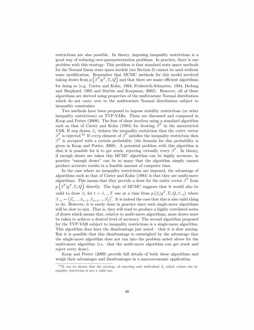
restrictions are also possible. In theory, imposing inequality restrictions is agood way of reducing over-parameterization problems. In practice, there is oneproblem with this strategy. This problem is that standard state space methodsfor the Normal linear state space models (see Section 3) cannot be used withoutsome modi�cation. Remember that MCMC methods for this model involvedtaking draws from p

��T jyT ;�; Q

�and that there are many e¢ cient algorithms

for doing so (e.g. Carter and Kohn, 1994, Fruhwirth-Schnatter, 1994, DeJongand Shephard, 1995 and Durbin and Koopman, 2002). However, all of thesealgorithms are derived using properties of the multivariate Normal distributionwhich do not carry over to the multivariate Normal distribution subject toinequality constraints.Two methods have been proposed to impose stability restrictions (or other

inequality restrictions) on TVP-VARs. These are discussed and compared inKoop and Potter (2009). The �rst of these involves using a standard algorithmsuch as that of Carter and Kohn (1994) for drawing �T in the unrestrictedVAR. If any drawn �t violates the inequality restriction then the entire vector�T is rejected.23 If every element of �T satis�es the inequality restriction then�T is accepted with a certain probability (the formula for this probability isgiven in Koop and Potter, 2009). A potential problem with this algorithm isthat it is possible for it to get stuck, rejecting virtually every �T . In theory,if enough draws are taken this MCMC algorithm can be highly accurate, inpractice �enough draws� can be so many that the algorithm simply cannotproduce accurate results in a feasible amount of computer time.In the case where no inequality restrictions are imposed, the advantage of

algorithms such as that of Carter and Kohn (1994) is that they are multi-movealgorithms. This means that they provide a draw for the entire vector �T from

p��T jyT ;�; Q

�directly. The logic of MCMC suggests that it would also be

valid to draw �t for t = 1; ::; T one at a time from p��tjyT ;�; Q; ��t

�where

��t =��01; ::; �t�1; �t+1; ::; �

0T

�0. It is indeed the case that this is also valid thing

to do. However, it is rarely done in practice since such single-move algorithmswill be slow to mix. That is, they will tend to produce a highly correlated seriesof draws which means that, relative to multi-move algorithms, more draws mustbe taken to achieve a desired level of accuracy. The second algorithm proposedfor the TVP-VAR subject to inequality restrictions is a single-move algorithm.This algorithm does have the disadvantage just noted �that it is slow mixing.But it is possible that this disadvantage is outweighed by the advantage thatthe single-move algorithm does not run into the problem noted above for themulti-move algorithm (i.e. that the multi-move algorithm can get stuck andreject every draw).Koop and Potter (2009) provide full details of both these algorithms and

weigh their advantages and disadvantages in a macroeconomic application.

23 It can be shown that the strategy of rejecting only individual �t which violate the in-equality restriction is not a valid one.

46

4.1.4 Dynamic Mixture Models

Another way of tightening the parameterization of the TVP-VAR is through thedynamic mixture model approach of Gerlach, Carter and Kohn (2000). Thishas recently been used in models of relevance for empirical macroeconomics inGiordani, Kohn and van Dijk (2007) and Giordani and Kohn (2008) and appliedto TVP-VARs in Koop, Leon-Gonzalez and Strachan (2009).To explain the usefulness of dynamic mixture modelling for TVP-VAR analy-

sis, return to the general form for the Normal linear state space model givenin (28) and (29) and remember that this model depended on so-called systemmatrices, Zt, Qt, �t, Wt and �t. Dynamic mixture models allow for any orall of these system matrices to depend on an s � 1 vector eKt. Gerlach, Carterand Kohn (2000) discuss how this speci�cation results in a mixtures of Normalsrepresentation for yt and, hence, the terminology dynamic mixture (or mix-ture innovation) model arises. The contribution of Gerlach, Carter and Kohn(2000) is to develop an e¢ cient algorithm for posterior simulation for this classof models. The e¢ ciency gains occur since the states are integrated out andeK =

� eK1; ::; eKT

�0is drawn unconditionally (i.e. not conditional on the states).

A simple alternative algorithm would involve drawing from the posterior for eKconditional on �T (and the posterior for �T conditional on eK). Such a strat-egy can be shown to produce a chain of draws which is very slow to mix. TheGerlach, Carter and Kohn (2000) algorithm requires only that eKt be Markov

(i.e. p� eKtj eKt�1; ::; eK1

�= p

� eKtj eKt�1

�) and is particularly simple if eKt is a

discrete random variable. We will not provide details of their algorithm here,but refer the reader to Gerlach, Carter and Kohn (2000) or Giordani and Kohn(2008). This algorithm is available on the Matlab website associated with thismonograph.The dynamic mixture framework can be used in many ways in empirical

macroeconomics, here we illustrate one useful way. Consider the following TVP-VAR:

yt = Zt�t + "t,

and

�t+1 = �t + ut;

where "t is i.i.d. N (0;�) and ut is i.i.d. N�0; eKtQ

�. This model is exactly the

same as the TVP-VAR of Section 4.1, except for the error covariance matrix inthe state equation. Let eKt 2 f0; 1g and assume a hierarchical prior for it of thefollowing form:

p� eKt = 1

�= q:

p� eKt = 0

�= 1� q

47

where q is an unknown parameter.24

This is a simple example of a dynamic mixture model. It has the propertythat:

�t+1 = �t + ut if eKt = 1

�t+1 = �t if eKt = 0:

In words, the VAR coe¢ cients can change at time t (if eKt = 1), but can alsoremain constant (if eKt = 0) and q is the probability that the coe¢ cients change.eKt and q are estimated in a data-based fashion. Thus, this model can have thefull �exibility of the TVP-VAR if the data warrant it (in the sense that it canselect eKt = 1 for t = 1; ::; T ). But it can also select a much more parsimoniousrepresentation. In the extreme, if eKt = 0 for t = 1; ::; T then we have the VARwithout time-varying parameters.This simple example allows either for all the VAR coe¢ cients to change

at time t (if eKt = 1) or none (if eKt = 0). More sophisticated models canallow for some parameters to change but not others. For instance, eKt couldbe a vector of M elements, each being applied to one of the equations in theVAR. Such a model would allow the VAR coe¢ cients in some equations tochange, but remain constant in other equations. In models with multivariatestochastic volatility, eKt could contain elements which control the variation inthe measurement error covariance matrix, �t. This avenue is pursued in Koop,Leon-Gonzalez and Strachan (2009). Many other possibilities exist (see, e.g., thetime-varying dimension models of Chan, Koop, Leon-Gonzalez and Strachan,2009) and the advantage of the dynamic mixture framework is that there existsa well-developed, well-understood set of MCMC algorithms that make Bayesianinference straightforward.

4.2 TVP-VARs with Stochastic Volatility

Thus far, we have focussed on the homoskedastic TVP-VAR, assuming the er-ror covariance matrix, � to be constant. However, we have argued above (seeSection 3.3) that volatility issues are often very important in empirical macro-economics. Thus, in most cases, it is important to allow for multivariate stochas-tic volatility in the TVP-VAR. Section 3.3.2 discusses multivariate stochasticvolatility, noting that there are many possible speci�cations for �t. Particu-lar approaches used in Cogley and Sargent (2005) and Primiceri (2005) are de-scribed in detail. All that we have to note here is that either of these approaches(or any other alternative) can be added to the homoskedastic TVP-VAR.With regards to Bayesian inference using MCMC methods, we need only

add another block to our algorithm to draw �t for t = 1; ::; T . That is,with the homoskedastic TVP-VAR we saw how an MCMC algorithm involv-

ing p�Q�1jyT ; �T

�, p��T jyT ;�; Q

�and p

���1jyT ; �T

�could be used. When

24This speci�cation for eKt is Markov in the degenerate sense that an independent processis a special case of Markov process.

48

adding multivariate stochastic volatility, the �rst of these densities is unchanged.

The second, p��T jyT ;�; Q

�, becomes p

��T jyT ;�1; ::;�T ; Q

�which can be

drawn from using any of the algorithms (e.g. Carter and Kohn, 1994) for the

Normal linear state space model mentioned previously. Finally, p���1jyT ; �T

�is replaced by p

���11 ; ::;��1T jyT ; �T

�. Draws from this posterior conditional

can be taken as described in Section 3.3.2.

4.3 Empirical Illustration of Bayesian Inference in TVP-VARs with Stochastic Volatility

We continue our empirical illustration of Section 4.1.1 which involved a ho-moskedastic TVP-VAR. All details of the empirical are as in Section 4.1.1 ex-cept we additionally allow for multivariate stochastic volatility as in Primiceri(2005). The prior for the parameters relating to the multivariate stochasticvolatility are speci�ed as in Primiceri (2005).For the sake of brevity, we do not present impulse responses (these are similar

to those presented in Primiceri, 2005). Instead we present information relatingto the multivariate stochastic volatility. Figure 6 presents the time-varyingstandard deviations of the errors in the three equations of our TVP-VAR (i.e.the posterior means of the square roots of the diagonal element of �t). Figure5 shows that there is substantial time variation in the error variances in allequations. In particular, it can be seen that 1970s was a very volatile periodfor the US economy, while the monetarist experiment of the early 1980s is alsowith instability. However, after the early 1980s volatility is greatly reduced inall equations. This latter period has come to be known as the Great Moderationof the business cycle.

49

Figure 5: Time-varying volatilities of errors in the three equations ofthe TVP-VAR

5 Factor Methods

The VAR and TVP-VAR methods we have discussed so far are typically usedwhen the number of variables in the model is relatively small (e.g. three or fourand rarely more than ten).25 However, in most modern economies, the macro-economist will potentially have dozens or hundreds of time series variables towork with. Especially when forecasting, the researcher wants to include as muchinformation as possible, and it can be desirable to work with as many variablesas possible. This can lead to models with a large number of variables and a pro-liferation of parameters. Accordingly, researchers have sought ways of extract-ing the information in data sets with many variables while, at the same time,keeping the model parsimonious. Beginning with Geweke (1977) factor modelshave been the most common way of achieving this goal (see Stock and Wat-son 2006 for a recent survey). Applications such as Forni and Reichlin (1998),Stock and Watson (1999, 2002), Bernanke and Boivin (2003), have popularizedfactor methods among macroeconomists and Geweke and Zhou (1996), Otrok

25An important exception is Banbura, Giannone and Reichlin (2008) which uses BayesianVARs (with time-invariant coe¢ cients) with up to 130 variables

50

and Whiteman (1998) and Kose, Otrok and Whiteman (2003), among manyothers, stimulated the interest of Bayesians. Papers such as Bernanke, Boivinand Eliasz (2005) and Stock and Watson (2005) have combined factor methodswith VAR methods. More recently, papers such as Del Negro and Otrok (2008)and Korobilis (2009a) provide further TVP extensions to these models. In thissection, we will describe dynamic factor models and their extensions to factoraugmented VARs (FAVARs) and TVP-FAVARs. As we shall see, these modelscan be interpreted as state space models and Bayesian MCMC algorithms thatuse our previously-discussed algorithms for state space models can be used.

5.1 Introduction

We will retain our notation where yt is an M � 1 vector of time series variables,but now M will be very large and let yit denote a particular variable. A simplestatic factor model is (see Lopes and West, 2004):

yt = �0 + �ft + "t; (49)

The key aspect of the factor model is the introduction of ft which is a q � 1vector of unobserved latent factors (where q << M) which contains informationextracted from all theM variables. The factors are common to every dependentvariable (i.e. the same ft occurs in every equation for yit for i = 1; :::;M), butthey may have di¤erent coe¢ cients (� which is aM�q matrix of so-called factorloadings). Also, the equation for every dependent variable has its own intercept(i.e. �0 isM�1 vector of parameters). "t is i.i.d. N (0;�) although, for reasonsexplained below, typically � is restricted to be a diagonal matrix. Di¤erentfactor models arise from the assumptions about the factors. For example, thesimplest case would be to assume that the factors come from a standard Normaldensity, ft � N (0; I). This implies that the covariance matrix of the observeddata can be written as:

var(y) = ��0 +�:

Alternatively, if we assume that the factors have a (not necessarily diagonal)covariance matrix �f , the decomposition becomes

var(y) = ��f�0 +�:

Even in this simple static framework, many extensions are possible. Forexample, Pitt and Shephard (1999) assume a factor stochastic volatility speci�-cation (i.e. a diagonal factor covariance matrix �ft which varies over time, withdiagonal elements following a geometric random walk). West (2003) uses SSVSon the parameters (�0; �).We write out these covariance matrices to illustrate the identi�cation issues

which arise in factor models. In general, var(y) will have M(M+1)2 elements

which can be estimated. However, without further restrictions, � and � (or�;�f and �) will have many more elements than this. The popular restrictionthat � is a diagonal matrix implies that all the commonalities across variables

51

occur through the factors and that the individual elements of "t are purely shockswhich are idiosyncratic to each variable. But additional identifying restrictionsare typically required. Lopes and West (2004) and Geweke and Zhou (1996)give a clear explanation of why identi�cation is not achieved in the simple factormodel. Below we will discuss more �exible factor models, but we stress thatthis added �exibility requires the imposition of more identi�cation restrictions.There is not a single, universally agreed-upon method for achieving identi�cationin these models. Below, we make particular choices that have been used in theliterature, but note that others are possible.

5.2 The Dynamic Factor Model

In macroeconomics, it is common to extend the static factor model to allow forthe dynamic properties which characterize macroeconomic variables. This leadsus to dynamic factor models (DFMs). A popular DFM is:

yit = �0i + �ift + "itft = �1ft�1 + ::+�pft�p + "

ft

"it = �i1"it�1 + ::+ �ipi"it�pi + uit

; (50)

where ft is de�ned as in (49), �i which is a 1� q vector of factor loadings. Also,the equation for every dependent variable has its own intercept, �0i. The errorin each equation, "it, may be autocorrelated, as speci�ed in the third equation in(50) which assumes uit to be i.i.d. N

�0; �2i

�. The vector of factors is assumed

to follow a VAR process with "ft being i.i.d. N�0;�f

�. The errors, uit are

independent over i; t and of "ft .Many slight modi�cations of the DFM given in (50) have been used in the

literature. But this speci�cation is a popular one so we will discuss factor modelsusing this framework. Note that it incorporates many identifying assumptionsand other assumptions to ensure parsimony. In particular, the assumption that�f = I is a common identifying assumption.26 If �f is left unrestricted, thenit is impossible to separately identify �i and �f . Similarly, the identifyingassumption that uit is uncorrelated with ujt (for i 6= j) and "ft is a standardone which assures that the co-movements in the di¤erent variables in yt arisesfrom the factors. Even with these assumptions, there is a lack of identi�cationsince the �rst equation of (50) can be replaced by:

yit = �0i + �iC0Cft + "it;

where C is any orthonormal matrix.27 Thus, (50) is observationally equivalentto a model with factors Cft and factor loadings �iC 0. One way of surmountingthis issue is to impose restrictions on �i (as is done below in our empiricalexample). A further discussion of various DFMs and identi�cation is provided,

26However, if (as below and in Pitt and Shephard, 1999) the researcher wishes to allow forfactor stochastic volatility then this identifying assumption cannot be made and an alternativeone is necessary.27An orthonormal matrix has the property that C0C = I.

52

e.g., in Stock and Watson (2005). See also Sentana and Fiorentini (2001) for adeeper discussion of identi�cation issues.To simplify the following discussion, we will assume the errors in the mea-

surement equation are not autocorrelated (i.e. "it are i.i.d. N�0; �2i

�and, thus,

�i1 = :: = �ipi = 0). We do this not because the extension to autocorrelated er-rors is empirically unimportant (it may be important), but because it involves astraightforward addition of other blocks to the MCMC algorithm of a standardform. That is, adding AR (or ARMA) errors to a regression model such as the�rst equation of (50) involves standard methods (see, e.g., Chib and Greenberg,1994). To be precise, the Chib and Greenberg (1994) algorithm will producedraws of �i1; ::; �ipi and these can be plugged into the usual quasi-di¤erencingoperator for AR models and this operator can be applied to the �rst equation in(50). The methods described below can then be used to draw all the other para-meters of this model, except that yit and ft will be replaced by quasi-di¤erencedversions.

5.2.1 Replacing Factors by Estimates: Principal Components

Before discussing a full Bayesian analysis of the DFM which (correctly) treatsft as a vector of unobserved latent variables, it is worth noting a simple approx-imation that may be convenient in practice. This approximation is used, e.g.,in Koop and Potter (2004). It involves noting that the DFM has approximatelythe same structure as the regression model:

yit = �0i + e�0ift + ::+ e�pift�p + e"it: (51)

Thus, if ft were known we could use Bayesian methods for the multivariateNormal regression model to estimate or forecast with the DFM.However, it is common to use principal components methods to approximate

ft.28 Hence, approximate methods for Bayesian analysis of the DFM can becarried out by simply replacing ft (51) by a principal components estimate andusing regression methods.

5.2.2 Treating Factors as Unobserved Latent Variables

It is also not di¢ cult to treat the factors as unobserved latent variables usingBayesian methods for state space models that were discussed in Section 3. Thisis particularly easy to see if we ignore the AR structure of the errors in themeasurement equation and write the DFM as

yit = �0i + �ift + "itft = �1ft�1 + ::+�pft�p + "

ft

(52)

for i = 1; ::;M where "it is i.i.d. N�0; �2i

�and "ft is i.i.d. N

�0;�f

�: In this

form it can be seen clearly that the DFM is a Normal linear state space model of28 If Y is the T�M matrix containing all the variables and W is theM�q matrix containing

the eigenvectors corresponding to the q largest eigenvalues of Y 0Y , then F = YW producesan estimate of the matrix of the factors.

53

the form given in (28) and (29). Thus all the methods for posterior simulationintroduced in Section 3 can be used to carry out Bayesian inference. In thefollowing we provide some additional detail about the steps involved.Note �rst that, conditional on the model�s parameters, �f ;�1; ::;�p; �0i; �i; �2i

for i = 1; ::;M , any of the standard algorithms for state space models such asthat of Carter and Kohn (1994) can be used to draw the factors. But con-ditional on the factors, the measurement equations are just M Normal linearregression models. Next note that the assumption that "it is independent of"jt for i 6= j means that the posteriors for �0i; �i; �2i in the M equations areindependent over i and, hence, the parameters for each equation can be drawnone at a time. Finally, conditional on the factors, the state equation becomes aVAR and the methods for Bayesian analysis in VARs of Section 2 can be used.Thus, every block in the resulting Gibbs sampler takes a standard form (e.g. noMetropolis-Hastings steps are required). Details on the derivations for this orrelated models can be found in many places, including Geweke and Zhou (1996),Kim and Nelson (1999), Lopes and West (2004) or Del Negro and Schorfheide(2010). Lopes and West (2004) discusses the choice of q, the number of factors.The preceding paragraph describes a correct MCMC algorithm that involves

blocks taken from MCMC algorithms described previously in this monograph.However, the fact that this algorithm draws the model�s parameters conditionalon the factors has been found by Chib, Nardari, and Shephard (2006) and Chanand Jeliazkov (2009) to lead to poor MCMC performance. That is, the sequenceof draws produced by the algorithm can be highly autocorrelated, meaning thata large number of draws can be required to achieve accurate estimates. Thesepapers provide alternative algorithms which integrate out the factors and, thus,do not run into this problem.

5.2.3 Impulse Response Analysis in the DFM

In our discussion of impulse response analysis in VAR models, we emphasizedhow it is typically done based on a structural VAR:

C0yt = c0 +

pXj=1

Cjyt�j + ut

or C (L) yt = c0 + ut where ut is i.i.d. N (0; I), C (L) = C0 �Pp

j=1 CjLp and

L is the lag operator. In fact, impulse responses are coe¢ cients in the vectormoving averaging (VMA) representation:

yt = ec0 + C (L)�1 ut;where ec0 is a vector of intercepts (ec0 = C (L)�1 c0). To be precise, the responseof the ith variable to the jth structural error h periods in the future, will be the(ij)

th element of the VMA coe¢ cient matrix on ut�h. This makes clear thatwhat is required for impulse response analysis is a VMA representation and amethod for structurally identifying shocks through a choice of C0.

54

With the DFM, we can obtain the VMA representation for yt. By substi-tuting the state equation in (52) into the measurement equation we can obtain:

yt = "t + �� (L)�1"ft

= B (L) �t

where � (L) = I � �1L � :: � �pLp and, for notational simplicity, we havesuppressed the intercept and are still assuming "t to be serially uncorrelated.Adding such extensions is conceptually straightforward (e.g. implying "t�1; ::; "t�pwould be included in the VMA representation).In the VMA form it can be seen that standard approaches to impulse re-

sponse analysis run into trouble when the DFM is used since the errors in theVMA are a combination of the measurement equation errors, "t, and the stateequation errors, "ft . For instance, in the VAR it is common to identify the struc-tural shocks by assuming C0 to be a lower-triangular matrix. If the interest ratewere the last element of yt this would ensure that the error in the interest rateequation had no immediate e¤ect on the other variables thus identifying it as amonetary policy shock under control of the central bank (i.e. the shock will beproportional to the change in interest rates). With the DFM, a monetary policyshock de�ned by assuming C0 to be lower triangular will not purely re�ect theinterest rate change, but will re�ect the change in the interest rate and relevantelement of "ft . Thus, impulse response analysis in DFMs is problematic: it is dif-�cult to identify an economically-sensible structural shock to measure impulseresponses to. This motivates the use of FAVARs. In one sense, these are simplya di¤erent form for writing the DFM but implicitly involve a restriction whichallows for economically-sensible impulse response analysis.29

5.3 The Factor Augmented VAR (FAVAR)

DFMs are commonly used for forecasting. However, interest in combining thetheoretical insights provided by VARs with factor methods�ability to extractinformation in large data sets motivates the development of factor augmentedVARs or FAVARs. For instance, a VAR with an identifying assumption whichisolates a monetary policy shock can be used to calculate impulse responseswhich measure the e¤ect of monetary policy. As we have seen, such theoreticalinsights are hard to obtain in the DFM. However, VARs typically involve only afew variables and it is possible that this means important economic informationis excluded.30 This suggests that combining factor methods, which extract theinformation in hundreds of variables, with VAR methods might be productive.

29This is the interpretation of the FAVAR given by Stock and Watson (2005) who begin bywriting the FAVAR as simply being a DFM written in VAR form.30As an example, VARs with a small number of variables sometimes lead to counter-intuitive

impulse responses such as the commonly noted price puzzle (e.g. where increases in interestrates seem to increase in�ation). Such puzzles often vanish when more variables are includedin the VAR suggesting that VARs with small numbers of variables may be mis-speci�ed.

55

This is done in papers such as Bernanke, Boivin and Eliasz (2005) and Belvisoand Milani (2006).The FAVAR modi�es a DFM such as (52) by adding other explanatory vari-

ables to the M measurement equations:

yit = �0i + �ift + irt + "it; (53)

where rt is a kr�1 vector of observed variables. For instance, Bernanke, Boivinand Eliasz (2005) set rt to be the Fed Funds rate (a monetary policy instrument)and, thus, kr = 1. All other assumptions about the measurement equation arethe same as for the DFM.The FAVAR extends the state equation for the factors to also allow for rt to

have a VAR form. In particular, the state equation becomes:�ftrt

�= e�1� ft�1

rt�1

�+ ::+ e�p� ft�p

rt�p

�+ e"ft (54)

where all state equation assumptions are the same as for the DFM with the

extension that e"ft is i.i.d. N �0; e�f� :We will not describe the MCMC algorithm for carrying out Bayesian infer-

ence in the FAVAR since it is very similar to that for the DFM.31 That is, (53)and (54) is a Normal linear state space model and, thus, standard methods (e.g.from Carter and Kohn, 1994) described in Section 3 can be used to draw thelatent factors (conditional on all other model parameters). Conditional on thefactors, the measurement equations are simply univariate Normal linear regres-sion models for which Bayesian inference is standard. Finally, conditional onthe factors, (54) is a VAR for which Bayesian methods have been discussed inthis monograph.

5.3.1 Impulse Response Analysis in the FAVAR

With the FAVAR, impulse responses of all the variables in yt to the shocksassociated with rt can be calculated using standard methods. For instance, ifrt is the interest rate and, thus, the error in its equation is the monetary policyshock, then the response of any of the variables in yt to the monetary policyshock can be calculated using similar methods as for the VAR. To see this notethat the FAVAR model can be written as:

�ytrt

�=

�� 0 1

��ftrt

�+ e"t;�

ftrt

�= e�1� ft�1

rt�1

�+ ::+ e�p� ft�p

rt�p

�+ e"ft

31The working paper version of Bernanke, Boivin and Eliasz (2005) has an appendix whichprovides complete details. See also the Matlab manual on the website associated with thismonograph.

56

where e"t = ("0t; 0)0 and is anM�kr matrix containing the is. As for the DFMmodel, for notational simplicity, we have suppressed the intercept and assumed"t to be serially uncorrelated. Adding such extensions is straightforward.

If we write the second equation in VMA form as�ftrt

�= e� (L)�1 e"ft

(where e� (L) = I � e�1L � :: � e�Lp) and substitute into the �rst equation, weobtain:

�ytrt

�=

�� 0 1

� e� (L)�1 e"ft + e"t= eB (L) �t:

Thus, we have a VMA form which can be used for impulse response analysis. Butconsider the last kr elements of �t which will be associated with the equationsfor rt. Unlike with the DFM, these VMA errors are purely the errors associatedwith the VAR for rt. This can be seen by noting that the last kr elements of e"tare zero and thus the corresponding elements of �t will only re�ect correspondingelements of e"ft which are errors in equations having rt as dependent variables.Unlike in the DFM, they do not combine state equation errors with measurementequation errors. For instance, if rt is an interest rate and structural identi�cationis achieved by assuming C0 (see equation 14) to be lower-triangular, then thestructural shock to the interest rate equation is truly proportional to a changein the interest rate and the response to such a monetary policy shock has aneconomically-sensible interpretation.Remember that, as with any factor model, we require identi�cation restric-

tions (e.g. principal components methods implicitly involve an identi�cationrestriction that the factors are orthogonal, but other restrictions are possible).In order to do structural impulse response analysis, additional identi�cation re-strictions are required (e.g. that C0 is lower-triangular). Note also that therestrictions such as C0 being lower triangular are timing restrictions and mustbe thought about carefully. For instance, Bernanke, Boivin and Eliasz (2005)divide the elements of yt into blocks of �slow variables� (i.e. those which areslow to respond to a monetary policy shock) and �fast variables�as part of theiridenti�cation scheme.

5.4 The TVP-FAVAR

In this monograph, we began by discussing Bayesian VAR modelling, beforearguing that it might be desirable to allow the VAR coe¢ cients to vary overtime. This led us to the homoskedastic TVP-VAR. Next, we argued that it isusually empirically important to allow for multivariate stochastic volatility. Wecan go through exactly the same steps with the FAVAR resulting in a TVP-FAVAR. Several speci�cations have been proposed, including Del Negro andOtrok (2008) and Korobilis (2009a). However, just as with TVP-VARs, it is

57

worth stressing that TVP-FAVARs can be over-parameterized and that care-ful incorporation of prior information or the imposing of restrictions (e.g. onlyallowing some parameters to vary over time) can be important in obtainingsensible results. Completely unrestricted versions of them can be di¢ cult toestimate using MCMC methods since they involve so many di¤erent state equa-tions (i.e. one set for the factors and others to model the evolution of theparameters).A very general speci�cation for the TVP-FAVAR is given in Korobilis (2009a)32

who replaces (53) and (54) by

yit = �0it + �itft + itrt + "it; (55)

and �ftrt

�= e�1t� ft�1

rt�1

�+ ::+ e�pt� ft�p

rt�p

�+ e"ft (56)

and assumes each "it follows a univariate stochastic volatility process and var�e"ft � =e�ft has a multivariate stochastic volatility process of the form used in Primiceri

(2005). Finally, the coe¢ cients (for i = 1; ::;M) �0it; �it; it; e�1t; ::; e�pt are al-lowed to evolve according to random walks (i.e. state equations of the sameform as 46 complete the model). All other assumptions are the same as for theFAVAR.We will not describe the MCMC algorithm for this model other than to note

that it simply adds more blocks to the MCMC algorithm for the FAVAR. Theseblocks are all of forms previously discussed in this monograph. For instance,the error variances in the measurement equations are drawn using the univariatestochastic volatility algorithm of Section 3.3.1. The algorithm of Section 3.3.2can be used to draw e�ft . The coe¢ cients �0it; �it; it; e�1t; ::; e�pt are all drawnusing the algorithm of Section 3.2, implemented in a very similar fashion as inthe TVP-VAR. In short, as with so many models in empirical macroeconomics,Bayesian inference in the TVP-FAVAR proceeds by putting together an MCMCalgorithm involving blocks from several simple and familiar algorithms.

5.5 Empirical Illustration of Factor Methods

To illustrate Bayesian inference in FAVARs and TVP-FAVAR models, we use adata set of 115 quarterly US macroeconomic variables spanning 1959Q1 though2006Q3. Following common practice in this literature, we transform all variablesto be stationary. For brevity, we do not list these variables here nor describe therequired stationarity transformations. These details are provided in the manualon the website associated with this monograph.The FAVAR is given in (53) and (54). It requires the choice of variables

to isolate in rt and we use the same variables as in our previous VAR and

32The model of Korobilis (2009a) is actually a slight extension of this since it includes adynamic mixture aspect similar to that presented in Section 4.1.3.

58

TVP-VAR empirical illustrations: in�ation, unemployment and the interest rate.Consequently, our FAVAR is the same tri-variate VAR used in previous empiricalillustrations, augmented with factors, ft, which are extracted from a large setof macroeconomic and �nancial variables.We use principal components methods to extract the �rst two factors which

are used in the FAVAR (q = 2) and two lags in the factor equation (p = 2).33 Theuse of principal components methods ensures identi�cation of the model since itnormalizes all factors to have mean zero and variance one. For the FAVAR werequire a prior for the parameters �f ;�1; ::;�p; �0i; �i; �2i for i = 1; ::;M . Fulldetails of this (relatively noninformative) prior are provided in the manual onthe website associated with this monograph.To carry out impulse response analysis we require additional identifying

assumptions. With regards to the equations for rt, we adopt the same identifyingassumptions as in our previous empirical illustrations. These allow us to identifya monetary policy shock. With regards to the variables in yt, su¢ ce it to notehere is that we adopt the same assumptions as Bernanke, Boivin and Eliasz(2005). The basic idea of their identifying scheme is described in Section 5.2.3above.Figures 6 and 7 plot impulse responses to the monetary policy shock for

the FAVAR. Figure 6 plots impulse responses for the main variables which areincluded in rt. The patterns in Figure 6 are broadly similar to those obtained inour empirical illustration using VARs (compare Figure 6 to Figure 4). However,the magnitudes of the impulse responses are somewhat di¤erent. Here we are�nding more evidence that a monetary policy shock will decrease in�ation. Fig-ure 7 plots the response of a few randomly selected variables to the monetarypolicy shock.34

33These choices are only illustrative. In a substantive empirical exercise, the researcherwould select these more carefully (e.g. using model selection methods such discussed previouslyin this monograph).34See the manual on the website associated with this monograph for a de�nition of the

abbreviations used in Figures 7 and 10. Brie�y GDPC96 is GDP, GSAVE is savings, PRFI isprivate residential �xed investment, MANEMP is employment in manufacturing, AHEMAN isearnings in manufacturing, HOUST is housing starts, GS10 is a 10 year interest rate, EXJPUSis the Japanese-US exchange rate, PPIACO is a producer price index, OILPRICE is the oilprice, HHSNTN is an index of consumer expectations and PMNO is the NAPM orders index.All impulse responses are to the original untransformed versions of these variables.

59

Figure 6: Posterior of impulse responses of main variables to monetarypolicy shock

60

Figure 7: Posterior of impulse responses of selected variables to monetarypolicy shock

We now present results for a TVP-FAVAR de�ned in (55) and (56), but withthe restriction that the parameters in the measurement equation are constantover time.35 The (relatively noninformative) prior we use is described in themanual on the website associated with this monograph.Figure 8 plots the posterior means of the standard deviations of the errors

in the two equations where the factors are the dependent variable and the threeequations where rt are the dependent variables. It can be seen that there issubstantive evidence of variation in volatilities (in particular, for equation forthe �rst factor). The bottom three panels of Figure 8 look similar to Figure 5and indicate the substantial increase in volatility associated with the 1970s andearly 1980s preceding the Great Moderation of the business cycle. However,this pattern is somewhat muted relative to Figure 5 since the inclusion of thefactors means that the standard deviation of the errors becomes smaller.35We do this since it is di¢ cult to estimate time variation in coe¢ cients in both the mea-

surement and state equation without additional restrictions or very strong prior information.

61

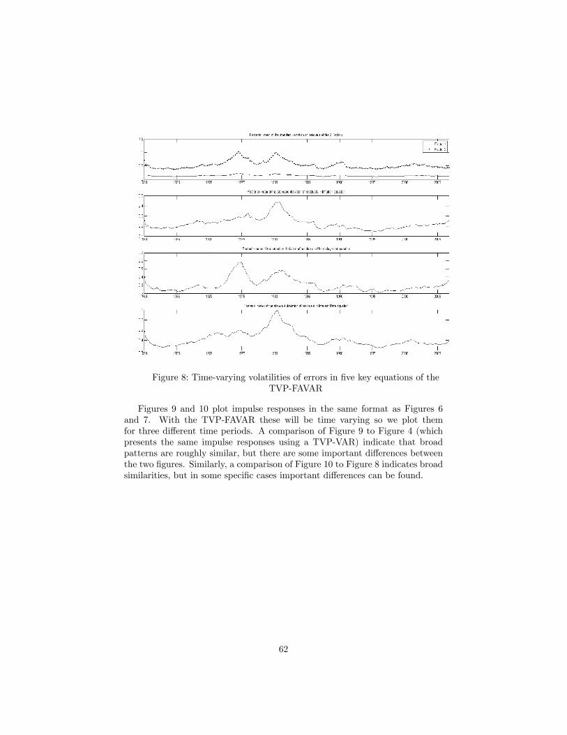
Figure 8: Time-varying volatilities of errors in �ve key equations of theTVP-FAVAR

Figures 9 and 10 plot impulse responses in the same format as Figures 6and 7. With the TVP-FAVAR these will be time varying so we plot themfor three di¤erent time periods. A comparison of Figure 9 to Figure 4 (whichpresents the same impulse responses using a TVP-VAR) indicate that broadpatterns are roughly similar, but there are some important di¤erences betweenthe two �gures. Similarly, a comparison of Figure 10 to Figure 8 indicates broadsimilarities, but in some speci�c cases important di¤erences can be found.

62

Figure 9: Posterior of impulse responses of main variables to monetary policyshock at di¤erent times

63

Figure 10: Posterior means impulse responses of selected variables tomonetary policy shock at di¤erent times

6 Conclusion

In this monograph, we have discussed VARs, TVP-VAR, FAVARs and TVP-FAVARs, including versions of these models with multivariate stochastic volatil-ity. These classes of models have become very popular with empirical macro-economists since they allow for insight into the relationships between macroeco-nomic variables in a manner which lets the data speak in a relatively uncon-strained manner. However, the cost of working with such unconstrained modelsis that they risk being over-parameterized. Accordingly, researchers have foundit desirable to impose soft or hard restrictions on these models. Soft restrictionstypically involve shrinking coe¢ cients towards a particular value (usually zero)whereas hard ones involve the imposition of exact restrictions. Bayesian meth-ods have been found to be an attractive and logically consistent way of handlingsuch restrictions.We have shown have Bayesian inference can be implemented in a variety of

ways in these models, with emphasis on speci�cations that are of interest to thepractitioner. Apart from the simplest of VARs, MCMC algorithms are required.This monograph describes these algorithms in a varying degree of detail. We

64

draw the reader�s attention to the website associated with this monograph whichcontains Matlab code for most of the models described above. A manual onthis website provides a complete listing of all formulae used in each MCMCalgorithm. Thus, our aim has been to provide a complete set of Bayesian toolsfor the practitioner interested in a wide variety of models commonly used inempirical macroeconomics.

65

ReferencesAn, S. and Schorfheide, F. (2007). �Bayesian analysis of DSGE models,�

Econometric Reviews, 26, 113-172.Asai, M., McAleer, M. and Yu, J. (2006). �Multivariate stochastic volatility:

A review,�Econometric Reviews, 25, 145-175.Ballabriga, F., Sebastian, M. and Valles, J. (1999). �European asymme-

tries,�Journal of International Economics, 48, 233-253.Banbura, M., Giannone, D. and Reichlin, L. (2010). �Large Bayesian VARs,�

Journal of Applied Econometrics, 25, 71-92.Belviso, F. and Milani, F. (2006). �Structural factor augmented VARs

(SFAVARs) and the e¤ects of monetary policy,� Topics in Macroeconomics,6, 2.Berg, A., Meyer, R. and Yu, J. (2004). �Deviance information criterion

for comparing stochastic volatility models,�Journal of Business and EconomicStatistics, 22, 107-120.Bernanke, B. and Boivin, J. (2003). �Monetary policy in a data-rich envi-

ronment,�Journal of Monetary Economics, 50, 525-546.Bernanke, B., Boivin, J. and Eliasz, P. (2005). �Measuring monetary pol-

icy: A Factor augmented vector autoregressive (FAVAR) approach,�QuarterlyJournal of Economics, 120, 387-422.Bernanke, B. and Mihov, I. (1998). �Measuring monetary policy,�Quarterly

Journal of Economics, 113, 869-902.Boivin, J. and Giannoni, M. (2006). �Has monetary policy become more

e¤ective?�Review of Economics and Statistics, 88, 445-462.Canova, F. (2007). Methods for Applied Macroeconomic Research published

by Princeton University Press.Canova, F. (1993). �Modelling and forecasting exchange rates using a Bayesian

time varying coe¢ cient model,� Journal of Economic Dynamics and Control,17, 233-262.Canova, F. and Ciccarelli, M. (2009). �Estimating multi-country VAR mod-

els,�International Economic Review, 50, 929-959.Canova, F. and Ciccarelli, M. (2004). �Forecasting and turning point predic-

tions in a Bayesian panel VAR model,�Journal of Econometrics, 120, 327-359.Canova, F. and Gambetti, L. (2009). �Structural changes in the US econ-

omy: Is there a role for monetary policy?�Journal of Economic Dynamics andControl, 33, 477-490.Carlin, B. and Chib, S. (1995). �Bayesian model choice via Markov chain

Monte Carlo methods,� Journal of the Royal Statistical Society, Series B, 57,473-84.Carter, C. and Kohn, R. (1994). �On Gibbs sampling for state space mod-

els,�Biometrika, 81, 541�553.Chan, J.C.C. and Jeliazkov, I. (2009). �E¢ cient simulation and integrated

likelihood estimation in state space models,� International Journal of Mathe-matical Modelling and Numerical Optimisation, 1, 101-120.Chan, J.C.C., Koop, G., Leon-Gonzalez, R. and Strachan, R. (2010). �Time

varying dimension models,�manuscript available at http://personal.strath.ac.uk/gary.koop/.

66

Chib, S. and Greenberg, E. (1994). �Bayes inference in regression modelswith ARMA(p,q) errors,�Journal of Econometrics, 64, 183-206.Chib, S. and Greenberg, E. (1995). �Hierarchical analysis of SUR models

with extensions to correlated serial errors and time-varying parameter models,�Journal of Econometrics, 68, 339-360.Chib, S. and Jeliazkov, I. (2001). �Marginal likelihood from the Metropolis-

Hastings output," Journal of the American Statistical Association, 96, 270-281.Chib, S. and Jeliazkov, I. (2005). �Accept-reject Metropolis-Hastings sam-

pling and marginal likelihood estimation," Statistica Neerlandica, 59, 30-44.Chib, S., Nardari, F. and Shephard, N. (2002). �Markov chain Monte Carlo

methods for stochastic volatility models,� Journal of Econometrics, 108, 281-316.Chib, S., Nardari, F. and Shephard, N. (2006). �Analysis of high dimensional

multivariate stochastic volatility models,� Journal of Econometrics, 134, 341-371.Chib, S., Omori, Y. and Asai, M. (2009). �Multivariate stochastic volatility,�

pages 365-400 in Handbook of Financial Time Series, edited by T. Andersen,R. David, J. Kreiss and T. Mikosch. Berlin: Springer-Verlag.Chib, S. and Ramamurthy, S. (2010). �Tailored Randomized Block MCMC

Methods with Application to DSGE Models,� Journal of Econometrics, 155,19-38.Chipman, H., George, E. and McCulloch, R. (2001). �Practical implemen-

tation of Bayesian model selection,�pages 67-116 in Model Selection, edited byP. Lahiri. Volume 38, IMS Lecture Notes.Christiano, L., Eichenbaum, M. and Evans, C. (1999). �Monetary shocks:

What have we learned and to what end?�, pages 65-148 in Handbook of Macro-economics, vol. 1A, edited by J. Taylor and M. Woodford. New York: Elsevier.Ciccarelli, M. and Rebucci, A., (2002). �The transmission mechanism of

European monetary policy: Is there heterogeneity? Is it changing over time?,�International Monetary Fund working paper, WP 02/54.Cogley, T. and Sargent, T. (2001). �Evolving post-World War II in�ation

dynamics,�NBER Macroeconomic Annual, 16, 331-373.Cogley, T. and Sargent, T. (2005). �Drifts and volatilities: Monetary policies

and outcomes in the post WWII U.S,�Review of Economic Dynamics, 8, 262-302.DeJong, P. and Shephard, N. (1995). �The simulation smoother for time

series models,�Biometrika, 82, 339-350.Del Negro, M. and Otrok, C. (2008). �Dynamic factor models with time

varying parameters: Measuring changes in international business cycles,�Fed-eral Reserve Bank of New York Sta¤ Report no. 326.Del Negro, M. and Schorfheide, F. (2004). �Priors from general equilibrium

models for VARs,�International Economic Review, 45, 643-673.Del Negro, M. and Schorfheide, F. (2010). �Bayesian macroeconometrics,�

to appear in the Handbook of Bayesian Econometrics, edited by J. Geweke, G.Koop and H. van Dijk. Oxford: Oxford University Press.

67

Doan, T., Litterman, R. and Sims, C. (1984). �Forecasting and conditionalprojection using realistic prior distributions,�Econometric Reviews, 3, 1-144.Doucet, A., Godsill, S. and Andrieu, C. (2000). �On sequential Monte Carlo

sampling methods for Bayesian �ltering,�Statistics and Computing, 10, 197-208.Durbin, J. and Koopman, S. (2001). Time Series Analysis by State Space

Methods. Oxford: Oxford University Press.Durbin, J. and Koopman, S. (2002). �A simple and e¢ cient simulation

smoother for state space time series analysis,�Biometrika, 89, 603-616.Fernandes-Villaverde, J. (2009). �The econometrics of DSGE models,�Penn

Institute for Economic Research working paper 09-008.Fernandez, C., Ley, E. and Steel, M. (2001). �Benchmark priors for Bayesian

model averaging,�Journal of Econometrics, 100, 381-427.Forni, M. and Reichlin, L. (1998). �Let�s get real: A factor analytic approach

to disaggregated business cycle dynamics,�Review of Economic Studies, 65, 453-473.Fruhwirth-Schnatter, S. (1994). �Data augmentation and dynamic linear

models,�Journal of Time Series Analysis, 15, 183�202.Fruhwirth-Schnatter, S. and Wagner, H. (2008). �Marginal likelihoods for

non-Gaussian models using auxiliary mixture sampling,�Computational Statis-tics and Data Analysis, 52, 4608-4624.Gelfand, A. and Dey, D. (1994). �Bayesian model choice: Asymptotics and

exact calculations,� Journal of the Royal Statistical Society Series B, 56, 501-514.George, E., Sun, D. and Ni, S. (2008). �Bayesian stochastic search for VAR

model restrictions,�Journal of Econometrics, 142, 553-580.Geweke, J. (1977). �The dynamic factor analysis of economic time series,�

in Latent Variables in Socio-economic Models, edited by D. Aigner and A. Gold-berger, Amsterdam: North Holland.Geweke, J. (1996). �Bayesian reduced rank regression in econometrics,�

Journal of Econometrics, 75, 121-146.Geweke, J. and Amisano, J. (2010). �Hierarchical Markov normal mixture

models with applications to �nancial asset returns,�Journal of Applied Econo-metrics, forthcoming.Geweke, J. and Keane, M. (2007). �Smoothly mixing regressions,�Journal

of Econometrics, 138, 252-291.Geweke, J. and Zhou, G. (1996). �Measuring the pricing error of the arbi-

trage pricing theory,�Review of Financial Studies, 9, 557-587.Giordani, P. and Kohn, R. (2008). �E¢ cient Bayesian inference for mul-

tiple change-point and mixture innovation models,� Journal of Business andEconomic Statistics, 26, 66-77.Giordani, P., Pitt, M. and Kohn, R. (2010). �Time series state space mod-

els,�to appear in the Handbook of Bayesian Econometrics, edited by J. Geweke,G. Koop and H. van Dijk. Oxford: Oxford University Press.Giordani, P., Kohn, R. and van Dijk, D. (2007). �A uni�ed approach to

nonlinearity, structural change and outliers,�Journal of Econometrics, 137, 112-133.

68

Green, P. (1995). �Reversible jump Markov chain Monte Carlo computationand Bayesian model determination,�Biometrika, 82, 711-32.Groen, J., Paap, R. and Ravazzolo, F. (2008). �Real-time in�ation forecast-

ing in a changing world,�Erasmus University manuscript, 2008.Harvey, A. (1989). Forecasting, Structural Time Series Models and the

Kalman Filter, Cambridge University Press: Cambridge.Ingram, B. and Whiteman, C. (1994). �Supplanting the Minnesota prior -

Forecasting macroeconomic time series using real business cycle model priors,�Journal of Monetary Economics, 49, 1131-1159.Jacquier, E., Polson, N. and Rossi, P. (1994). �Bayesian analysis of stochas-

tic volatility,�Journal of Business and Economic Statistics, 12, 371-417.Johannes, M. and Polson, N. (2009). �Particle �ltering,�pages 1015-1030 in

Handbook of Financial Time Series, edited by T. Andersen, R. David, J. Kreissand T. Mikosch. Berlin: Springer-Verlag.Kadiyala, K. and Karlsson, S. (1997). �Numerical methods for estimation

and inference in Bayesian VAR models,�Journal of Applied Econometrics, 12,99-132.Kim, C. and Nelson, C. (1999). State Space Models with Regime Switching.

Cambridge: MIT Press.Kim, S., Shephard, N. and Chib, S. (1998). Stochastic volatility: likelihood

inference and comparison with ARCH models, Review of Economic Studies, 65,361-93.Koop, G. (1992). �Aggregate shocks and macroeconomic �uctuations: A

Bayesian approach,�Journal of Applied Econometrics, 7, 395-411.Koop, G. (1996). �Parameter uncertainty and impulse response analysis,�

Journal of Econometrics, 72, 135-149.Koop, G. (2010). �Forecasting with medium and large Bayesian VARs,�

manuscript available at http://personal.strath.ac.uk/gary.koop/.Koop, G., Leon-Gonzalez, R. and Strachan, R. (2009). �On the evolution of

the monetary policy transmission mechanism,�Journal of Economic Dynamicsand Control, 33, 997�1017.Koop, G., Poirier, D. and Tobias, J. (2007). Bayesian Econometric Methods.

Cambridge: Cambridge University Press.Koop, G. and Potter, S. (2004). �Forecasting in dynamic factor models using

Bayesian model averaging,�The Econometrics Journal, 7, 550-565.Koop, G. and Potter, S. (2006). �The Vector �oor and ceiling model,�

Chapter 4 in Nonlinear Time Series Analysis of the Business Cycle, edited byC. Milas, P. Rothman and D. van Dijk in Elsevier�s Contributions to EconomicAnalysis series.Koop, G. and Potter, S. (2009). �Time varying VARs with inequality restric-

tions,�manuscript available at http://personal.strath.ac.uk/gary.koop/koop_potter14.pdf.Korobilis, D. (2009a). �Assessing the transmission of monetary policy shocks

using dynamic factor models,�University of Strathclyde, Discussion Papers inEconomics, No. 09-14.Korobilis, D. (2009b). �VAR forecasting using Bayesian variable selection,�

manuscript.

69

Kose, A., Otrok, C. and Whiteman, C. (2003). �International business cy-cles: World, region and country-speci�c factors,�American Economic Review,93, 1216-1239.Kuo, L. and B. Mallick. (1997). �Variable selection for regression models,�

Shankya: The Indian Journal of Statistics (Series B), 60, 65-81.Litterman, R. (1986). �Forecasting with Bayesian vector autoregressions �

Five years of experience,�Journal of Business and Economic Statistics, 4, 25-38.Lopes, H. and West, M. (2004). �Bayesian model assessment in factor analy-

sis,�Statistica Sinica, 14, 41-67.Lubik, T. and Schorfheide, F. (2004). �Testing for indeterminacy: An appli-

cation to U.S. monetary policy,�American Economic Review, 94, 190-217.McCausland, W., Miller, S. and Pelletier, D. (2007). �A new approach to

drawing states in state space models,� working paper 2007-06, Université deMontréal, Département de sciences économiques.Omori, Y., Chib, S., Shephard, N. and Nakajima, J. (2007). �Stochas-

tic volatility with leverage: Fast and e¢ cient likelihood inference,�Journal ofEconometrics, 140, 425-449.Otrok, C. and Whiteman, C. (1998). �Bayesian leading indicators: Mea-

suring and predicting economic conditions in Iowa,� International EconomicReview, 39, 997-1014.Paap, R. and van Dijk, H. (2003). �Bayes estimates of Markov trends in

possibly cointegrated series: An application to US consumption and income,�Journal of Business and Economic Statistics, 21, 547-563.Pitt, M. and Shephard, N. (1999). �Time varying covariances: a factor

stochastic volatility approach,� pages 547�570 in Bayesian Statistics, Volume6, edited by J. Bernardo, J.O. Berger, A.P. Dawid and A.F.M. Smith, Oxford:Oxford University Press.Primiceri. G., (2005). �Time varying structural vector autoregressions and

monetary policy,�Review of Economic Studies, 72, 821-852.Rubio-Ramirez, J., Waggoner, D. and Zha, T. (2010). �Structural vector

autoregressions: Theory of identi�cation and algorithms for inference,�Reviewof Economic Studies, forthcoming.Sentana, E. and Fiorentini, G. (2001). �Identi�cation, estimation and testing

of conditionally heteroskedastic factor models,� Journal of Econometrics, 102,143-164.Sims, C. (1993). �A nine variable probabilistic macroeconomic forecasting

model,�pp. 179-204 in J. Stock and M. Watson, eds., Business Cycles Indicatorsand Forecasting. University of Chicago Press for the NBER).Sims, C. (1980). �Macroeconomics and reality,�Econometrica, 48, 1�48.Sims, C. and Zha, T. (1998). �Bayesian methods for dynamic multivariate

models,�International Economic Review, 39, 949-968.Sims, C. and Zha, T. (2006). �Were there regime switches in macroeconomic

policy?�American Economic Review, 96, 54-81.Stock, J. and Watson, M., (1996). �Evidence on Structural Instability in

Macroeconomic Time Series Relations,�Journal of Business and Economic Sta-tistics, 14, 11-30.

70

Stock, J. and Watson, M., (1999). �Forecasting in�ation,�Journal of Mon-etary Economics, 44, 293-335.Stock, J. and Watson, M., (2002). �Macroeconomic forecasting using di¤u-

sion indexes,�Journal of Business and Economic Statistics, 20, 147-162.Stock, J. and Watson, M., (2005). �Implications of dynamic factor models

for VAR analysis,�National Bureau of Economic Research working paper 11467.Stock, J. and Watson, M., (2006). �Forecasting using many predictors,�pp.

515-554 in Handbook of Economic Forecasting, Volume 1, edited by G. Elliott,C. Granger and A. Timmerman, Amsterdam: North Holland.Stock, J. and Watson, M., (2008). �Forecasting in dynamic factor models

subject to structural instability,� in The Methodology and Practice of Econo-metrics, A Festschrift in Honour of Professor David F. Hendry, edited by J.Castle and N. Shephard, Oxford: Oxford University Press.Villani, M. (2009). �Steady-state prior for vector autoregressions,�Journal

of Applied Econometrics, 24, 630-650.West, M. (2003). �Bayesian factor regression models in the �large p, small

n�paradigm,�pages 723-732 in Bayesian Statistics, Volume 7, edited by J.M.Bernardo, M. Bayarri, J.O. Berger, A.P. Dawid, D. Heckerman, A.F.M. Smith,and M. West, Oxford: Oxford University Press.West, M. and Harrison, P. (1997). Bayesian Forecasting and Dynamic Mod-

els. Second edition. Berlin: Springer.

71