Bayesian Methods for Intensity Measure and Ground Motion ...
199
Bayesian Methods for Intensity Measure and Ground Motion Selection in Performance-Based Earthquake Engineering Somayajulu L. N. Dhulipala Dissertation submitted to the Faculty of the Virginia Polytechnic Institute and State University in partial fulfillment of the requirements for the degree of Doctor of Philosophy in Civil Engineering Madeleine M. Flint, Chair Matthew R. Eatherton Bruce R. Ellingwood Jennifer L. Irish Adrian Rodriguez-Marek February 11, 2019 Blacksburg, Virginia Keywords: Ground Motion Characterization, Information Theory, Copulas, Markov Chain Monte Carlo Copyright 2019, Somayajulu L. N. Dhulipala
Transcript of Bayesian Methods for Intensity Measure and Ground Motion ...
Bayesian Methods for Intensity Measure and Ground Motion Selection in
Performance-Based Earthquake Engineering
Somayajulu L. N. Dhulipala
Dissertation submitted to the Faculty of the
Virginia Polytechnic Institute and State University
in partial fulfillment of the requirements for the degree of
Doctor of Philosophy
in
Civil Engineering
Madeleine M. Flint, Chair
Matthew R. Eatherton
Bruce R. Ellingwood
Jennifer L. Irish
Adrian Rodriguez-Marek
February 11, 2019
Blacksburg, Virginia
Keywords: Ground Motion Characterization, Information Theory, Copulas,
Markov Chain Monte Carlo
Copyright 2019, Somayajulu L. N. Dhulipala
Bayesian Methods for Intensity Measure and Ground Motion Selection in
Performance-Based Earthquake Engineering
Somayajulu L. N. Dhulipala
(ABSTRACT)
The objective of quantitative Performance-Based Earthquake Engineering (PBEE) is design-ing buildings that meet the specified performance objectives when subjected to an earthquake.One challenge to completely relying upon a PBEE approach in design practice is the open-endednature of characterizing the earthquake ground motion by selecting appropriate ground motionsand Intensity Measures (IM)1 for seismic analysis. This open-ended nature changes the quantifiedbuilding performance depending upon the ground motions and IMs selected. So, improper groundmotion and IM selection can lead to errors in structural performance prediction and thus to poordesigns. Hence, the goal of this dissertation is to propose methods and tools that enable an informedselection of earthquake IMs and ground motions, with the broader goal of contributing toward arobust PBEE analysis. In doing so, the change of perspective and the mechanism to incorporateadditional information provided by Bayesian methods will be utilized.
Evaluation of the ability of IMs towards predicting the response of a building with precision andaccuracy for a future, unknown earthquake is a fundamental problem in PBEE analysis. Whereascurrent methods for IM quality assessment are subjective and have multiple criteria (hence makingIM selection challenging), a unified method is proposed that enables rating the numerous IMs.This is done by proposing the first quantitative metric for assessing IM accuracy in predicting thebuilding response to a future earthquake, and then by investigating the relationship between preci-sion and accuracy. This unified metric is further expected to provide a pathway toward improvingPBEE analysis by allowing the consideration of multiple IMs.
Similar to IM selection, ground motion selection is important for PBEE analysis. Consensuson the right input motions for conducting seismic response analyses is often varied and dependenton the analyst. Hence, a general and flexible tool is proposed to aid ground motion selection.General here means the tool encompasses several structural types by considering their sensitivitiesto different ground motion characteristics. Flexible here means the tool can consider additionalinformation about the earthquake process when available with the analyst. Additionally, in supportof this ground motion selection tool, a simplified method for seismic hazard analysis for a vector ofIMs is developed.
This dissertation addresses four critical issues in IM and ground motion selection for PBEE byproposing: (1) a simplified method for performing vector hazard analysis given multiple IMs; (2)a Bayesian framework to aid ground motion selection which is flexible and general to incorporatepreferences of the analyst; (3) a unified metric to aid IM quality assessment for seismic fragilityand demand hazard assessment; (4) Bayesian models for capturing heteroscedasticity (non-constantstandard deviation) in seismic response analyses which may further influence IM selection.
1Peak Ground Acceleration is an example; although, numerous other IMs such as Peak Ground Velocity, PeakGround Displacement, and Spectral Accelerations can be derived from an accelerogram.
Bayesian Methods for Intensity Measure and Ground Motion Selection in
Performance-Based Earthquake Engineering
Somayajulu L. N. Dhulipala
(GENERAL AUDIENCE ABSTRACT)
Earthquake ground shaking is a complex phenomenon since there is no unique way to assess itsstrength. Yet, the strength of ground motion (shaking) becomes an integral part for predicting thefuture earthquake performance of buildings using the Performance-Based Earthquake Engineering(PBEE) framework. The PBEE framework predicts building performance in terms of expectedfinancial losses, possible downtime, the potential of the building to collapse under a future earth-quake. Much prior research has shown that the predictions made by the PBEE framework areheavily dependent upon how the strength of a future earthquake ground motion is characterized.This dependency leads to uncertainty in the predicted building performance and hence its seismicdesign. The goal of this dissertation therefore is to employ Bayesian reasoning, which takes intoaccount the alternative explanations or perspectives of a research problem, and propose robustquantitative methods that aid IM selection and ground motion selection in PBEE
The fact that the local intensity of an earthquake can be characterized in multiple ways usingIntensity Measures (IM; e.g., peak ground acceleration) is problematic for PBEE because it leadsto different PBEE results for different choices of the IM. While formal procedures for selecting anoptimal IM exist, they may be considered as being subjective and have multiple criteria makingtheir use difficult and inconclusive. Bayes rule provides a mechanism called change of perspectiveusing which a problem that is difficult to solve from one perspective could be tackled from a differ-ent perspective. This change of perspective mechanism is used to propose a quantitative, unifiedmetric for rating alternative IMs. The immediate application of this metric is aiding the selectionof the best IM that would predict the building earthquake performance with least bias.
Structural analysis for performance assessment in PBEE is conducted by selecting ground mo-tions which match a target response spectrum (a representation of future ground motions). Thedefinition of a target response spectrum lacks general consensus and is dependent on the analysts’preferences. To encompass all these preferences and requirements of analysts, a Bayesian targetresponse spectrum which is general and flexible is proposed. While the generality of this Bayesiantarget response spectrum allow analysts select those ground motions to which their structures arethe most sensitive, its flexibility permits the incorporation of additional information (preferences)into the target response spectrum development.
This dissertation addresses four critical questions in PBEE: (1) how can we best define groundmotion at a site?; (2) if ground motion can only be defined by multiple metrics, how can we easilyderive the probability of such shaking at a site?; (3) how do we use these multiple metrics to se-lect a set of ground motion records that best capture the site’s unique seismicity; (4) when thoserecords are used to analyze the response of a structure, how can we be sure that a standard linearregression technique accurately captures the uncertainty in structural response at low and highlevels of shaking?

Acknowledgments
This dissertation is supported by the National Science Foundation through award number 1455466
and partly by the Virginia Tech College of Engineering Pratt Fellowship. This financial support is
gratefully acknowledged.
First and foremost, I express my sincere gratitude to my advisor, Prof. Madeleine Flint, for
providing the opportunity to work with her and for supporting my development as an indepen-
dent researcher. The critical pieces of advice Madeleine gave were instrumental to ensuring that
my research stayed on the right track. The emphasis she put on my research communication is
extraordinary, and this has positively influenced, and will continue to influence, my explanation of
difficult concepts to an audience. The various opportunities she provided to present my research at
meetings and conferences, and the collaborations she let me establish within and outside of Virginia
Tech significantly contributed to my professional development. Madeleine’s support was crucial for
my success as a doctoral student, and for this, I am indebted to her.
Prof. Adrian Rodriguez-Marek also has significantly contributed to my development as a
scholar. He introduced me to site response analysis which is widely practiced in both academia
and the industry. The enthusiasm he showed towards my research reciprocated in me with greater
intensity. He also provided opportunities for professional development and collaborations. I am,
therefore, grateful towards everything Prof. Rodriguez-Marek has done for me.
Prof. Jack Baker has unconditionally reviewed and provided a thorough critique of several as-
pects of my research. In addition, the emphasis he places on high quality and high impact research
is very motivating. My committee members’ (Profs. Matthew Eatherton, Bruce Ellingwood, Jen-
nifer Irish) critique has helped me very much to think from a big-picture perspective. In addition,
the valuable feedback they provided on my thesis is much appreciated. Profs. Shyam Ranganathan,
Guney Olgun, Martin Chapman, and Ioannis Koutromanos are thanked for providing stimulating
research discussions.
I thank Chenxi (2x), Sai, Adrian, Mohsen, Helen, Gary, Aimane, Jeena, Soheil, Karim, Mahdi,
Ali, and Javier for their freindship as my office mates. I specially thank Anjaney, Abhishek, Esh-
iv

wari, and Japsimran for their friendship as my roommates. Finally, but most importantly, I thank
my family for their support.
v
Contents
List of Figures xiii
List of Tables xx
1 Introduction 1
1.1 Performance-Based Earthquake Engineering design philosophy . . . . . . . . . . . . 2
1.2 Motivation of this thesis . . . . . . . . . . . . . . . . . . . . . . . . . . . . . . . . . . 4
1.3 The importance of Intensity Measure selection for Performance-Based Earthquake
Engineering . . . . . . . . . . . . . . . . . . . . . . . . . . . . . . . . . . . . . . . . . 7
1.3.1 State of the art in Intensity Measure selection . . . . . . . . . . . . . . . . . . 7
1.3.2 Need for quantitative methods for Intensity Measure selection . . . . . . . . . 8
1.4 Ground motion selection for Performance-Based Earthquake Engineering . . . . . . . 9
1.4.1 State-of-the-art in ground motion selection . . . . . . . . . . . . . . . . . . . 9
1.4.2 Need for a holistic and a flexible ground motion selection target . . . . . . . . 10
1.5 Research objectives . . . . . . . . . . . . . . . . . . . . . . . . . . . . . . . . . . . . . 11
1.6 Organization . . . . . . . . . . . . . . . . . . . . . . . . . . . . . . . . . . . . . . . . 12
2 Background 14
2.1 State of Research in Intensity Measure Selection . . . . . . . . . . . . . . . . . . . . 14
2.1.1 Efficiency . . . . . . . . . . . . . . . . . . . . . . . . . . . . . . . . . . . . . . 14
2.1.2 Sufficiency . . . . . . . . . . . . . . . . . . . . . . . . . . . . . . . . . . . . . . 16
vi
2.1.3 Hazard Computability . . . . . . . . . . . . . . . . . . . . . . . . . . . . . . . 17
2.2 State of Research in Ground Motion Selection Tools . . . . . . . . . . . . . . . . . . 18
2.2.1 Seismic Hazard Analysis and Uniform Hazard Spectrum . . . . . . . . . . . . 18
2.2.2 Conditional Mean Spectrum . . . . . . . . . . . . . . . . . . . . . . . . . . . . 20
2.2.3 Generalized Conditioning Intensity Measure . . . . . . . . . . . . . . . . . . . 21
2.3 Bayesian Methods: A Primer . . . . . . . . . . . . . . . . . . . . . . . . . . . . . . . 22
2.3.1 Bayes rule . . . . . . . . . . . . . . . . . . . . . . . . . . . . . . . . . . . . . . 22
2.3.2 Prior distributions, Conjugate priors, and Non-informative priors . . . . . . . 24
2.3.3 Markov Chain Monte Carlo sampling . . . . . . . . . . . . . . . . . . . . . . . 27
2.3.4 Information Theory in Bayesian Analysis . . . . . . . . . . . . . . . . . . . . 30
2.4 Summary . . . . . . . . . . . . . . . . . . . . . . . . . . . . . . . . . . . . . . . . . . 31
3 Application of Bayesian methods in PBEE: Capturing heteroscedasticity in seis-
mic response analyses 32
3.1 Introduction . . . . . . . . . . . . . . . . . . . . . . . . . . . . . . . . . . . . . . . . . 32
3.2 Algorithms considered to capture heteroscedasticity . . . . . . . . . . . . . . . . . . 34
3.2.1 The frequentist algorithm . . . . . . . . . . . . . . . . . . . . . . . . . . . . . 34
3.2.2 The Bayesian algorithm . . . . . . . . . . . . . . . . . . . . . . . . . . . . . . 35
3.3 Case study description . . . . . . . . . . . . . . . . . . . . . . . . . . . . . . . . . . . 39
3.4 Results . . . . . . . . . . . . . . . . . . . . . . . . . . . . . . . . . . . . . . . . . . . . 40
3.4.1 Sa(T1 = 1.33s) as conditioning IM . . . . . . . . . . . . . . . . . . . . . . . . 41
3.4.2 PGA as conditioning IM . . . . . . . . . . . . . . . . . . . . . . . . . . . . . . 43
3.5 Impact on fragility estimation . . . . . . . . . . . . . . . . . . . . . . . . . . . . . . . 45
vii
3.6 Conclusions . . . . . . . . . . . . . . . . . . . . . . . . . . . . . . . . . . . . . . . . . 45
4 A unified metric for the quality assessment of scalar intensity measures that
characterize an earthquake 48
4.1 Introduction . . . . . . . . . . . . . . . . . . . . . . . . . . . . . . . . . . . . . . . . . 48
4.2 Case study description . . . . . . . . . . . . . . . . . . . . . . . . . . . . . . . . . . . 52
4.2.1 Structure description . . . . . . . . . . . . . . . . . . . . . . . . . . . . . . . . 52
4.2.2 Intensity measures, structural response quantities and seismological parameters 52
4.2.3 Site description . . . . . . . . . . . . . . . . . . . . . . . . . . . . . . . . . . . 53
4.2.4 Ground motion record sets . . . . . . . . . . . . . . . . . . . . . . . . . . . . 53
4.3 Site hazard consistent conditional independence assessment of alternative Intensity
Measures . . . . . . . . . . . . . . . . . . . . . . . . . . . . . . . . . . . . . . . . . . 55
4.3.1 Mathematical description of the proposed approach . . . . . . . . . . . . . . 55
4.3.2 Empirical models relating EDP −IMi and EDP −IMi−φj and assumption
of normality . . . . . . . . . . . . . . . . . . . . . . . . . . . . . . . . . . . . . 59
4.3.3 Deaggregation given IM exceedence versus deaggregation given IM equivalence 60
4.3.4 IM conditional independence assessment using exact deaggregation . . . . . . 60
4.3.5 IM conditional independence assessment using approximate deaggregation . . 64
4.3.6 Exact and approximate marginal deaggregation probabilities at the real site . 66
4.4 Influence of ground motion record sets on sufficiency of scalar IMs . . . . . . . . . . 69
4.5 Relation between the sufficiency and the efficiency criterion of seismic IMs and their
unification . . . . . . . . . . . . . . . . . . . . . . . . . . . . . . . . . . . . . . . . . . 76
4.6 Summary and Conclusions . . . . . . . . . . . . . . . . . . . . . . . . . . . . . . . . . 79
5 A pre-configured solution to the problem of joint hazard estimation given a suite
viii
of seismic intensity measures 82
5.1 Introduction . . . . . . . . . . . . . . . . . . . . . . . . . . . . . . . . . . . . . . . . . 82
5.1.1 Prior research on vector hazard analysis . . . . . . . . . . . . . . . . . . . . . 83
5.1.2 Objectives of the present study . . . . . . . . . . . . . . . . . . . . . . . . . . 84
5.2 Background . . . . . . . . . . . . . . . . . . . . . . . . . . . . . . . . . . . . . . . . . 85
5.3 Features of seismic hazard deaggregation . . . . . . . . . . . . . . . . . . . . . . . . . 87
5.4 Vector deaggregation and vector hazard . . . . . . . . . . . . . . . . . . . . . . . . . 92
5.4.1 Manipulations to compute the vector hazard/deaggregation . . . . . . . . . . 95
5.4.2 Application to a hypothetical site surrounded by multiple fault sources . . . . 96
5.5 Application of the proposed vector hazard approach to a real site in Los Angeles, CA 98
5.6 Discussion of Intensity Measure correlation coefficients in relation to the proposed
vector hazard approach . . . . . . . . . . . . . . . . . . . . . . . . . . . . . . . . . . 101
5.7 Can the invariance property be utilized to directly compute scalar hazard curves
using new a GMPM/IM? . . . . . . . . . . . . . . . . . . . . . . . . . . . . . . . . . 104
5.8 Summary and Conclusions . . . . . . . . . . . . . . . . . . . . . . . . . . . . . . . . . 106
6 A Bayesian treatment of the Conditional Spectrum approach for ground motion
selection 108
6.1 Introduction . . . . . . . . . . . . . . . . . . . . . . . . . . . . . . . . . . . . . . . . . 108
6.2 Bayesian Conditional Spectrum . . . . . . . . . . . . . . . . . . . . . . . . . . . . . . 110
6.2.1 Ground motion modeling . . . . . . . . . . . . . . . . . . . . . . . . . . . . . 111
6.2.2 Ground motion model implementation . . . . . . . . . . . . . . . . . . . . . . 114
6.2.3 Conditioning at a spectral time period . . . . . . . . . . . . . . . . . . . . . . 115
6.3 Accounting for the M -R pair selection uncertainty from the deaggregation plot . . . 118
ix
6.3.1 M-R pair selection uncertainty in Los Angeles, CA . . . . . . . . . . . . . . . 119
6.3.2 M-R pair selection uncertainty at two other sites . . . . . . . . . . . . . . . . 120
6.4 Effects of tuning the priors to simulated ground motions on the Conditional Spectrum122
6.4.1 Motivation . . . . . . . . . . . . . . . . . . . . . . . . . . . . . . . . . . . . . 122
6.4.2 High risk ground motions in the NGA-West2 database . . . . . . . . . . . . . 123
6.4.3 Simulation of high-risk ground motions . . . . . . . . . . . . . . . . . . . . . 123
6.4.4 Combining the NGA-West2 and simulated ground motion sets . . . . . . . . 125
6.4.5 Simulation of the CS . . . . . . . . . . . . . . . . . . . . . . . . . . . . . . . . 127
6.5 Extending the Conditional Spectrum approach to a general class of structures . . . . 128
6.5.1 Motivation . . . . . . . . . . . . . . . . . . . . . . . . . . . . . . . . . . . . . 128
6.5.2 Multiple IM conditioning under the Bayesian CS . . . . . . . . . . . . . . . . 129
6.5.3 Vector deaggregation given the conditional IMs . . . . . . . . . . . . . . . . . 129
6.5.4 The CS under multiple IM conditioning . . . . . . . . . . . . . . . . . . . . . 129
6.6 Summary and Conclusions . . . . . . . . . . . . . . . . . . . . . . . . . . . . . . . . . 130
7 Conclusions and future recommendations 138
7.1 Summary . . . . . . . . . . . . . . . . . . . . . . . . . . . . . . . . . . . . . . . . . . 138
7.1.1 A unified metric for Intensity Measure quality assessment . . . . . . . . . . . 138
7.1.2 A pre-configured solution to vector seismic hazard analysis . . . . . . . . . . 140
7.1.3 A Bayesian modification to the Conditional Spectrum approach for ground
motion selection . . . . . . . . . . . . . . . . . . . . . . . . . . . . . . . . . . 142
7.2 Comments on the application of Bayesian methods in this dissertation . . . . . . . . 143
7.3 Critique of the present work . . . . . . . . . . . . . . . . . . . . . . . . . . . . . . . . 144
x
7.3.1 A unified metric for intensity measure selection in PBEE . . . . . . . . . . . 144
7.3.2 A pre-configured solution for vector probabilistic seismic hazard analysis . . . 145
7.3.3 A Bayesian implementation of the Conditional Spectrum approach for ground
motion selection . . . . . . . . . . . . . . . . . . . . . . . . . . . . . . . . . . 146
7.4 Looking forward: an integrated approach for intensity measure and ground motion
selection in PBEE . . . . . . . . . . . . . . . . . . . . . . . . . . . . . . . . . . . . . 146
Appendices 148
Appendix A Relation between IM efficiency and its ground motion record repre-
sentation capacity 149
Appendix B Vector seismic hazard and deaggregation: additional results 152
B.1 Vector hazard and deaggregation for the IMs Sa(1s), PGA, and PGV in LA, CA . . 152
B.2 Comparison between Gaussian and ‘t’ Copulas in predicting the vector seismic hazard153
Appendix C Posterior distributions of the parameter matrices α and Σ for the
Gibbs sampling MCMC scheme 156
C.1 Prior distributions for α and Σ . . . . . . . . . . . . . . . . . . . . . . . . . . . . . . 156
C.2 Posterior distributions for α and Σ . . . . . . . . . . . . . . . . . . . . . . . . . . . . 157
Appendix D Is the correlation structure between seismic intensity measures rup-
ture dependent? 158
D.1 Introduction . . . . . . . . . . . . . . . . . . . . . . . . . . . . . . . . . . . . . . . . . 158
D.2 Statistical testing to investigate the heteroscedasticity in IM prediction . . . . . . . . 160
D.3 Multivariate Heteroscedastic GMPM . . . . . . . . . . . . . . . . . . . . . . . . . . . 161
D.3.1 Model formulation . . . . . . . . . . . . . . . . . . . . . . . . . . . . . . . . . 161
xi

D.3.2 Results . . . . . . . . . . . . . . . . . . . . . . . . . . . . . . . . . . . . . . . 162
D.3.3 Evaluation using AIC and BIC . . . . . . . . . . . . . . . . . . . . . . . . . . 163
D.4 Conclusions . . . . . . . . . . . . . . . . . . . . . . . . . . . . . . . . . . . . . . . . . 164
Bibliography 166
xii
List of Figures
1.1 The PEER framework for Performance-Based Earthquake Engineering.
Abbreviations. IM: Intensity Measure, EDP: Engineering Demand Parameter, DS:
Damage State. . . . . . . . . . . . . . . . . . . . . . . . . . . . . . . . . . . . . . . . 3
1.2 Influence of Intensity Measure (IM) selection on the decision hazard in PBEE. . . . 6
1.3 Demonstration of the concepts of IM efficiency and sufficiency. (a) An efficient, but
not sufficient, IM may lead to precise (i.e., less dispersed) PBEE results but there
is no guarantee that these results are accurate. (b) A sufficient, but not efficient,
IM may lead to accurate PBEE results, but with more dispersion. In summary, both
efficiency and sufficiency are complementing attributes for an IM. . . . . . . . . . . 8
1.4 Demonstration of three popular target spectrum that aid in ground motion matching
and selection: (a) ASCE 7-16 (b) Uniform Hazard Spectrum (c) Conditional Mean
Spectrum conditioned at 1s at a site in Palo Alto, CA. The design level is 475-years
of return period. . . . . . . . . . . . . . . . . . . . . . . . . . . . . . . . . . . . . . . 10
2.1 Depiction of (a) IM efficiency and (b) IM sufficiency. . . . . . . . . . . . . . . . . . 16
2.2 (a) Illustration of PSHA. (b) Illustration of computing the UHS using PSHA results. 19
2.3 (a) Illustration of the CMS and the variability around it including an example set
of matched ground motions. (b) Illustration of an IM conditional distribution in the
GCIM approach including the Cumulative Distribution Function of an example set
of matched ground motions. . . . . . . . . . . . . . . . . . . . . . . . . . . . . . . . . 21
2.4 Influence of prior distribution on the posterior demonstrated using: (a) non-informative
flat prior; (b) informative prior. . . . . . . . . . . . . . . . . . . . . . . . . . . . . . . 27
xiii
2.5 (a) Example of a posterior distribution estimated using MCMC sampling. (b) Anal-
ogy of the Metropolis-Hastings algorithm with a person lost in a dark forest trying to
get to the camp site. It is noted that the camp site is well lit and the person has a
light meter. . . . . . . . . . . . . . . . . . . . . . . . . . . . . . . . . . . . . . . . . . 28
2.6 Convergence of the Metropolis-Hastings algorithm that starts from some arbitrary
point. Once convergence is achieved, the algorithm draws random samples from the
posterior. . . . . . . . . . . . . . . . . . . . . . . . . . . . . . . . . . . . . . . . . . . 29
3.1 Typical frequency distributions of IMs: (a) Sa(T1 = 1.33s) and (b) PGA used for
the analysis. . . . . . . . . . . . . . . . . . . . . . . . . . . . . . . . . . . . . . . . . . 40
3.2 Evaluation of the performance of frequentist and Bayesian algorithms in capturing
heteroscedasticity under the IM Sa(T1 = 1.33s) and for the EDPs: (a) Inter-story
Drift Ratio 1 (IDR1) (b) IDR4 (c) Roof Drift (d) Peak Floor Acceleration 1 (PFA1)
(e) PFA2 (f) PFA3. The circles represent conditional standard deviations obtained
through IDA. . . . . . . . . . . . . . . . . . . . . . . . . . . . . . . . . . . . . . . . . 42
3.3 Evaluation of the performance of frequentist and Bayesian algorithms in capturing
heteroscedasticity under the IM PGA and for the EDPs: (a) Inter-story Drift Ratio
1 (IDR1) (b) IDR4 (c) Roof Drift (d) Peak Floor Acceleration 1 (PFA1) (e) PFA2
(f) PFA3. The circles represent conditional standard deviations obtained through IDA. 44
3.4 Evaluation of the impact of heteroscedasticity on fragility estimation at roof drifts:
(a) 0.02 (b) 0.03 (c) 0.04 (d) 0.045. IDA refers to utilization of the variance func-
tional form from IDA results, and heteroscedasticity refers to use of the Bayesian
algorithm to capture the variance change. . . . . . . . . . . . . . . . . . . . . . . . . 46
4.1 (a) Conditional mean spectrum and fifty seven matched ground motions; (b) Vari-
ability in the target and sample conditional response spectrum . . . . . . . . . . . . . 55
4.2 Total Information Gain vs. response for alternative IMs evaluated at the hypothetical
site using the FEMA P695 far-field record set for the three seismological parameters
(M , R, and ε) in consideration . . . . . . . . . . . . . . . . . . . . . . . . . . . . . . 62
xiv
4.3 IDR4 regression residuals versus M under the FEMA P695 far-field record set for
IMs (a) Sa(T1 = 1.33s), (b) Sa(2s), and (c) PGV . Standard deviation in lnEDP
given lnIM (denoted as β in this figure), p-value and Information Gain with respect
to M are depicted. . . . . . . . . . . . . . . . . . . . . . . . . . . . . . . . . . . . . . 64
4.4 (a) Visualization of the approximate deaggregation procedure—the red lines corre-
spond to deaggregation probabilities at coarse IM levels and the surface corresponds
to continuously interpolated deaggregation probabilities; (b) Comparison of exact and
approximate Total Information Gains (TIG). . . . . . . . . . . . . . . . . . . . . . . 67
4.5 Comparison of exact and approximate marginal deaggregation probabilities at the real
site at an IM level of 0.35g (35 Cm/s for PGV ). . . . . . . . . . . . . . . . . . . . . 68
4.6 Influence of ground motion selection on sufficiency: TIGs for various IMs at the
real site considering the record set (a) FEMA P695 far-field (b) Medina-Krawinkler
LMSR-N (c) CS matched (no pulse) (d) CS matched (pulse). The most sufficient
IMs (least TIG) for various EDP -record set combinations are stated above each
EDP . In (c), the IM Sa(2s) has a TIG of 2.08 and 2.28 bits for PFA1 and
PFA4, respectively. . . . . . . . . . . . . . . . . . . . . . . . . . . . . . . . . . . . . 69
4.7 Sa(T1 = 1.33s) given Roof Drift > 0.04 distributions without and with considering
the seismological parameters (M , R, ε) for the record sets: (a) CS matched no pulse
set; (b) CS matched pulse set. The TIGs are also depicted. . . . . . . . . . . . . . . 72
4.8 Demand hazard curves computed without and with considering the seismological pa-
rameters (M , R, ε) for the EDP s Roof drift (a & b) IDR1 (c & d) IDR4 (e & f).
The combination of record set and IM is depicted within each sub-figure. The values
of Total Information Gain (TIG) and standard deviation in predicting lnEDP given
lnIM (βlnEDP |lnIM ) are also depicted. . . . . . . . . . . . . . . . . . . . . . . . . . . 74
xv
4.9 Demand hazard curves computed without and with considering the seismological pa-
rameters (M , R, ε) for the EDP s Joint Rotation (a & b) PFA1 (c & d) PFA4
(e & f). The combination of record set and IM is depicted within each sub-figure.
The values of Total Information Gain (TIG) and standard deviation in predicting
lnEDP given lnIM (βlnEDP |lnIM ) are also depicted. . . . . . . . . . . . . . . . . . . 75
4.10 Relation between standard deviation in structural response given IM (βlnEDP |lnIM )
and average Total Information Gain (TIG) for the EDP s, IMs, ground motion
record sets and structure considered in this study. where, ρ is the Pearson correlation
coefficient, and σ is the standard deviation in predicting ln TIG given ln βlnEDP |lnIM . 77
4.11 (a) Transformed values of lnβlnEDP |lnIM and lnTIG into the standard normal space;
(b) Exponent of the transformed values which are utilized to perform the Euclidean
distance with reference to the origin; (c) Histogram of natural logarithm of the Eu-
clidean distance—the unified metric—for various combinations of IMs, EDPs and
ground motion sets. . . . . . . . . . . . . . . . . . . . . . . . . . . . . . . . . . . . . . 79
5.1 Depiction of the logic-tree used for the hypothetical site considered in this study.
Only unique branches arising at each rightward step are represented (there are eight
final branches). A fraction along each of the branch arrows represents the weight
given to that rightward step. Abbreviations: Campbell-Bozorgnia 2008 (CB), Boore-
Atkinson 2008 (BA), Reverse fault (R), Normal fault (N). . . . . . . . . . . . . . . . 88
5.2 (a) Seismic hazard curves at hypothetical site for the IM Sa(2s) (b) Hazard deaggre-
gation at Sa(2s) > 0.5g. . . . . . . . . . . . . . . . . . . . . . . . . . . . . . . . . . . 89
5.3 λ(IM > x, Mj , Rj) with Sa(2s) level for M-R bins (6.45, 28Km) and (7.05, 16Km),
respectively, depicting the function’s monotonically decreasing nature. . . . . . . . . . 90
5.4 Invariance of deaggregations with the choice of IM for a low IM level (1e-6 g) . . . . 91
5.5 Aggregated conditional probability of IM exceedence for the IM Sa(2s) conditional on
M-R bins (6.45, 28Km) and (7.05, 16Km), respectively, at the hypothetical site . . . 92
xvi
5.6 (a) Joint aggregated conditional probability of IM exceedences for the IMs Sa(2s) and
PGA conditioned on M-R of (7.05, 16Km) (b) Joint deaggregation corresponding to
IM levels of 0.5g and 0.75g for Sa(2s) and PGA, respectively . . . . . . . . . . . . . 96
5.7 Vector hazard surface for the IMs Sa(2s) and PGA computed using a Gaussian Cop-
ula. The exact vector hazard analysis results are also provided for comparison purposes. 97
5.8 Conditional hazard curves for Sa(2s) computed using both Gaussian Copula (solid
lines) and exact vector hazard analysis (circles). These hazard curves are conditioned
on PGA exceedences of 0.25g, 0.75g, 2g, and 5g. . . . . . . . . . . . . . . . . . . . . 98
5.9 (a) Depiction of λ(IM > x,Mj , Rj) as a function of Sa(2s) level at the real site
in Los Angeles, CA for two M-R bins; (b) Low-IM-level deaggregation plot at this
site (PGA greater than 0.0001g); (c) Aggregate conditional probability of IM excee-
dence as function of Sa(2s) level for two M-R bins at this site; (d) Joint aggregate
conditional probability of IM exceedences for the two IMs Sa(2s) and PGA, and
conditional on a M-R combination 7− 12.5Km. . . . . . . . . . . . . . . . . . . . . . 101
5.10 (a) Vector hazard surface and the (b) Corresponding deaggregation conditional on
the IM levels (Sa(2s) > 0.45g, PGA > 0.75g) at the same site in Los Angeles, CA. . 102
5.11 PGA, SA correlations computed using the: (a) NGA-West2 and (b) NGA-East
databases. It is noted that the correlations are computed using a subset of these
databases and are not recommended for use in practice. . . . . . . . . . . . . . . . . 103
5.12 Comparison of hazard curve from OpenSHA with an approximate one obtained using
the invariance property of deaggregations for the IMs (a) Sa(2s) and (b) PGA. These
plots are for the same site in Los Angeles, CA. . . . . . . . . . . . . . . . . . . . . . 106
6.1 Comparison of the (a) Conditional Mean Spectrum and the (b) Conditional standard
deviation computed using Bayesian (using non-informative priors) and Frequentist
(Baker and Lee 2017) methodologies for a site in Los Angeles, CA. Similarity of the
results indicate an equivalence between the two approaches. . . . . . . . . . . . . . . . 117
xvii
6.2 Influence of variability within the deaggregation plots on the Conditional standard
deviation in the CS approach. It can be observed that more erratic mass distribu-
tion within the deaggregation plot has a greater impact on the Conditional standard
deviation as compared to the case where mean M-R values are used. . . . . . . . . . 120
6.3 (a) & (c) and (b) & (d) represent the Target Variabilities (Conditional standard de-
viation) for Bissell and Stanford sites, respectively. While (a) & (b) use the mean
values of M-R obtained from the deaggregation plot, (c) & (d) consider the M-R vari-
ability within these plots. In each plot, Conditional standard deviation is obtained
from three sources: using Bayesian methodology developed in this study, using Fre-
quentist methodology presented in Lin et al. (2013)Lin et al. (2013a) with BSSA
2014 GMPM, and data from Lin et al. (2013)Lin et al. (2013a). It is noted that the
data from Lin et al. (2013)Lin et al. (2013a) relies on three NGA-West1 GMPMs
for making the CS computations. . . . . . . . . . . . . . . . . . . . . . . . . . . . . . 133
6.4 (a) M − R distribution of earthquakes within the curtailed NGA-West2 set with
M > 6.5 and RJB < 20Km; these records correspond to 5.7% (250 records) of
the curtailed NGA-West2 set. Notice that M > 7.1 records are even more sparsely
populated. (b) M − R distribution of simulated records using EXSIM along with
NGA-West2 earthquakes. Notice that EXSIM simulations augment the curtailed
NGA-West2 dataset for M −R ranges where this set has sparsely populated records. 134
6.5 Comparison of the mean response spectrum obtained from the Curtailed NGA-West2
database (4390 records), the M > 6.5 &RJB < 20Km subset of NGA-West2 set (250
records), and the EXSIM simulated set (500 records). . . . . . . . . . . . . . . . . . . 134
6.6 Mean coefficient values across the spectral periods. Whereas the likelihoods and the
priors in this figure correspond to coefficient values inferred from the curtailed NGA-
West2 and the EXSIM simulated sets, respectively, posteriors correspond to values
obtained by combining these two sets using Bayes rule. . . . . . . . . . . . . . . . . . 135
xviii
6.7 Conditional Mean Spectrum and Conditional standard deviation((a),(c) and (b),(d),
respectively)
for Bissell and Stanford sites((a),(b) and (c),(d), respectively
)com-
puted using the curtailed NGA-West2 set with flat priors (solid pink plot) and the
same set combined with EXSIM priors (dashed green plot). . . . . . . . . . . . . . . 136
6.8 Conditional Mean Spectrum and Target Variaiblity when conditioned on the vector
IMs: Sa(0.67s), PGA ((a) and (b), respectively); PGV, PGA ((c) and (d),
respectively). Results for the corresponding scalar IM conditioning are also provided
for reference. IM , on the y-axis, indicates that conditioning is made on a vector of
IMs . . . . . . . . . . . . . . . . . . . . . . . . . . . . . . . . . . . . . . . . . . . . . 137
B.1 Vector hazard surface for the IMs PGV , Sa(1s), and (a) PGA > 0.1g (b) PGA >
2g. (c) Vector deaggregation for the IM levels PGV > 150Cm/s, PGA > 0.5g, Sa(1s) >
0.5g. AFE: Annual Frequency of Exceedance. . . . . . . . . . . . . . . . . . . . . . . 153
B.2 Comparison between the vector hazards obtained using a Gaussian Copula and a ‘t’-
Copula. Four IM combinations are considered: (a) PGV and PGA > 0.5g (b) PGV
and PGA > 2g (c) PGA and PGV > 150Cm/s (d) PGA and PGV > 300Cm/s. . . 155
D.1 (a) Variability in standards deviations in the NGA-West2 database subset for three
spectral periods: 0.1, 0.667, 2s. The vertical lines indicate the homoscedastic stan-
dard deviations. (b), (c), and (c): Variability in correlation coefficients for three
combinations of spectral periods. The vertical lines indicate the constant correla-
tions from the Baker-Jayaram correlation model. . . . . . . . . . . . . . . . . . . . . 165
xix
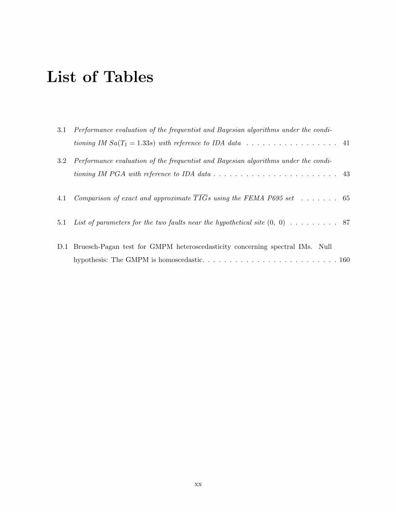
List of Tables
3.1 Performance evaluation of the frequentist and Bayesian algorithms under the condi-
tioning IM Sa(T1 = 1.33s) with reference to IDA data . . . . . . . . . . . . . . . . . 41
3.2 Performance evaluation of the frequentist and Bayesian algorithms under the condi-
tioning IM PGA with reference to IDA data . . . . . . . . . . . . . . . . . . . . . . . 43
4.1 Comparison of exact and approximate TIGs using the FEMA P695 set . . . . . . . 65
5.1 List of parameters for the two faults near the hypothetical site (0, 0) . . . . . . . . . 87
D.1 Bruesch-Pagan test for GMPM heteroscedasticity concerning spectral IMs. Null
hypothesis: The GMPM is homoscedastic. . . . . . . . . . . . . . . . . . . . . . . . . 160
xx

List of Abbreviations
AFE Annual Frequency of Exceedance
ASCE American Society for Civil Engineers
BA Boore and Atkinson
CB Campbell and Bozorginia
CCDF Complementary Cumulative Distribution Function
CDF Cumulative Distribution Function
CMS Conditional Mean Spectrum
CS Conditional Spectrum
EDP Engineering Demand Parameter
FEMA Federal Emergency Management Agency
GCIM Generalized Conditioning Intensity Measure
GLM Generalized Linear Model
GMPM Ground Motion Prediction Model
IDA Incremental Dynamic Analysis
IDR Inter-story Drift Ratio
IG Information Gain
IM Intensity Measure
JR Joint Rotation
KLD Kullback Leibler Divergence
xxi

MCMC Markov Chain Monte Carlo
MH Metropolis Hastings
NGA Next Generation Attenuation
OLS Ordinary Least Squares
PBEE Performance-Based Earthquake Engineering
PEER Pacific Earthquake Engineering Research
PFA Peak Floor Acceleration
PGA Peak Ground Acceleration
PGV Peak Ground Velocity
PSDA Probabilistic Seismic Demand Analysis
PSHA Probabilistic Seismic Hazard Analysis
RD Roof Drift
Sa(T1) Spectral acceleration at the fundamental period
TIG Total Information Gain
TV Target Variability
UHS Uniform Hazard Spectrum
USGS United States Geological Survey
xxii
Chapter 1
Introduction
Earthquakes are among the most uncertain and difficult natural hazards to prepare for. Between
1900 and 2011, earthquakes caused approximately 2.5 million fatalities and 2000 billion dollars
in economic losses around the world (Daniell et al., 2011)1. In the U.S., it is estimated that the
expected annual losses concerning earthquakes are around 6.1 billion dollars in 2017, which is a 10%
net increase since 2008 (USGS, 2017)2. With rapid urbanization and increased human development
in exposed territories, designing buildings to be resistant and resilient to earthquakes is more crucial
than ever. Performance-based design provides a way to achieve this objective by designing buildings
to meet certain performance objectives.
One challenge to completely relying on a performance-based design approach is the open-ended
nature of characterizing the earthquake ground motion by selecting appropriate ground motions and
Intensity Measures (IM; e.g., Peak Ground Acceleration) for seismic response analysis. This open-
ended nature changes the quantified building performance depending upon the ground motions and
IMs selected. Hence, this dissertation focuses on developing tools, inspired by Bayesian statistical
methods, that enable an informed selection of ground motions and the intensity measure for use in
performance-based engineering. Bayesian reasoning takes into account the alternative explanations
or perspectives of a research problem. This change of perspective, the flexibility to incorporate new
information, and the comprehensiveness in uncertainty quantification offered by Bayesian statistical
methods will be used to solve some key problems related to IM and ground motion selection.
1International dollars; Hybrid Natural Disaster Economic Conversion Index adjusted to April 2011.2U.S. dollars; inflation adjusted to 2014.
1

2 Chapter 1. Introduction
1.1 Performance-Based Earthquake Engineering design philoso-
phy
Earthquakes embody multiple levels of uncertainties ranging from their occurrences and intensities
to their effects, such as damages, losses, and recovery. Quantifying these uncertainties in terms
of decision variables such as costs, downtime or fatalities will aid in designing resistant and re-
silient buildings that meet owners’ requirements. For example, among a suite of building design
alternatives that maybe subjected to earthquakes, the alternative that is most likely to meet the
prescribed performance standards is selected. These performance standards are specified in terms
of decision-variable values corresponding to a design level; for example, the 2475-year return period
hazard level. The ability of the alternative designs to meet these standards is assessed through
a rigorous quantification of uncertainties associated with earthquakes and their effects. Broadly
speaking, this is known as a full performance-based approach for designing buildings.
Although the current design codes include a performance-based approach, the extent to which
they do is limited; that is, they do not follow the full approach. These codes set up the performance
goals for buildings ambiguously and qualitatively (Krawinkler, 1999). As an example, Table 1.5−1
of ASCE7 (2010) uses terms such as “low risk to human life”, “substantial risk to human life”, and
“maintain the functionality” to describe performance expectations. This qualitative description has
significantly limited the engineer’s ability to derive more performance from the designed buildings
as the design codes, at best, only intend to protect against the loss of life during an earthquake.
With the aim of achieving the full performance-based design to enable buildings to be cost-
effective, resilient, and sustainable (in addition to protecting lives during an earthquake), the
Pacific Earthquake Engineering Research (PEER) framework for Performance-Based Earthquake
Engineering (PBEE) was proposed (Moehle and Deierlein, 2004). The goal of PEER PBEE is to de-
scribe the seismic performance of buildings quantitatively in terms of continuous decision-variables
rather than subjective performance levels (this definition is mentioned in numerous studies on
performance-based engineering; for e.g., Bozorgnia and Bertero 2004; Flint et al. 2014). The PEER
PBEE framework constitutes four analysis stages, (1) ground motion, (2) structural response, (3)
building damage, and (4) decision variable, presented in Figure 1.1. The uncertainty in each stage is
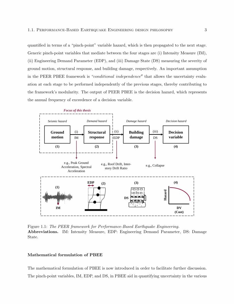
1.1. Performance-Based Earthquake Engineering design philosophy 3
quantified in terms of a “pinch-point” variable hazard, which is then propagated to the next stage.
Generic pinch-point variables that mediate between the four stages are (i) Intensity Measure (IM),
(ii) Engineering Demand Parameter (EDP), and (iii) Damage State (DS) measuring the severity of
ground motion, structural response, and building damage, respectively. An important assumption
in the PEER PBEE framework is “conditional independence′′ that allows the uncertainty evalu-
ation at each stage to be performed independently of the previous stages, thereby contributing to
the framework’s modularity. The output of PEER PBEE is the decision hazard, which represents
the annual frequency of exceedence of a decision variable.
Ground
motion
Structural
response
Building
damage
Seismic hazard
Decision
variable
Demand hazard Damage hazard Decision hazard
IM EDP DS
(1) (2) (3) (4)
(i) (ii) (iii)
Focus of this thesis
e.g., Peak Ground
Acceleration, Spectral
Acceleration
e.g., Roof Drift, Inter-
story Drift Ratioe.g., Collapse
IM
EDP
DS
DV
(Cost)
Ha
zard
(1)(2) (3) (4)
Figure 1.1: The PEER framework for Performance-Based Earthquake Engineering.Abbreviations. IM: Intensity Measure, EDP: Engineering Demand Parameter, DS: DamageState.
Mathematical formulation of PBEE
The mathematical formulation of PBEE is now introduced in order to facilitate further discussion.
The pinch-point variables, IM, EDP, and DS, in PBEE aid in quantifying uncertainty in the various
4 Chapter 1. Introduction
PBEE stages. An IM (e.g., peak ground acceleration, spectral acceleration) is used to quantify the
uncertainty in the ground motion as a hazard function(λ(IM)
)and also to facilitate uncertainty
quantification in structural response by correlating with an EDP. Likewise, an EDP (e.g., roof
drift of a building) is used to both quantify the uncertainty in structural response and to facilitate
quantifying uncertainty in building damage by correlating with the DS. Finally, the DS quantifies
uncertainty in building damage and correlates with the DV. These uncertainties and correlations
within the pinch-point variables are integrated sequentially in the order presented in Figure 1.1 to
express the earthquake risk in terms of an annual frequency of exceedence of the decision-variable(λ(DV )
). This statement is also mathematically represented in equation 1.1:
λ(DV ) =
∫im
∫edp
∑dsi
P (DV > y|DSi) P (DSi|EDP ) f(EDP |IM) dEDP dλ(IM) (1.1)
where P (.|.) and f(.|.) represent conditional probability and conditional probability density, respec-
tively, and they quantify the uncertainty in a pinch-point variable by considering its correlation
with a preceding variable.
The emphasis of this dissertation is on the ground motion and structural response stages in
PBEE (also refer to Figure 1.1). In particular, methods and tools that enable informed selection
of the IM and the associated ground motions at the intersection of these stages will be proposed.
As will be discussed further, appropriate ground motion and IM selection are contributing factors
to accurate uncertainty quantification not only of the structural response, but also of the decision-
variables.
1.2 Motivation of this thesis
The results of PBEE (i.e., the decision hazard) depend on the initial setup of the problem. Con-
ducting a PBEE analysis first requires a selection of the ground motion IM for performing a seismic
hazard analysis (phase 1 in Figure 1.1) and then a selection of the suitable ground motions for per-
forming structural response analyses in order to compute the demand hazard (phase 2 in Figure

1.2. Motivation of this thesis 5
1.1). The choice of the IM and ground motions, however, is open-ended, and the nature of this
selection is shown to strongly influence the decision hazard (Kohrangi et al., 2016c). An example of
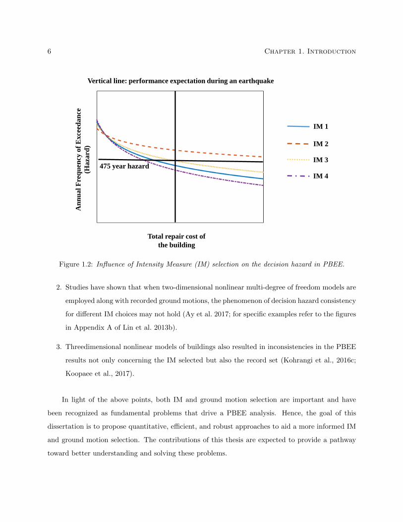
this is demonstrated in Figure 1.2 where the decision hazards computed using several IMs are incon-
sistent. In the middle of this Figure, the horizontal line represents the return period or the selected
hazard level of a decision-variable and the vertical line represents the performance expectation of
a building3. Whereas a few IMs indicate that the building satisfies the performance expectations,
others contradict this assertion. A similar problem exists with ground motion selection as well,
where the nature of the ground motions selected impacts the PBEE results (Koopaee et al., 2017).
From a broader perspective, employing PBEE in design practice requires a careful selection of
the IM and the ground motions to avoid a false sense of confidence on the building’s performance.
An inappropriate selection of the IM and the ground motions, may give an exaggerated represen-
tation of the building’s performance. This unconservative prediction in turn poses the possibility
that the designed building may not meet the fundamental performance expectation, i.e. life-safety,
let alone the others that PBEE aims to design for (e.g., losses and downtime). Alternatively, an
inappropriate IM and the ground motion selection may also lead to under representation of the
building’s performance, in which case, the total cost of the building will be larger than necessary.
There is a debate in the scientific literature over whether proper ground motion selection,
consistent with the seismic hazard at a site, could lead to the insensitivity of PBEE results to
the IM selected. For example, Bradley (2012a) and Bradley et al. (2015) show that careful record
selection, taking into account the seismic hazard levels at different values of a selected IM, leads to
not only consistency of decision hazards for different IM choices but also agreement of results with
a benchmark obtained through Monte-Carlo simulations4. However, the following points are noted
in this regard:
1. Such a consistency has been demonstrated for simplified models such as single degree of
freedom systems or using simulated ground motions at hypothetical sites with less complicated
seismic activity than real sites (Kwong and Chopra, 2016b).
3If the decision-variable is incurred costs during an earthquake, the designed building through PBEE should havelesser incurred cost than the performance expectation.
4It is to be noted that a Monte-Carlo approach for decision hazard computation, as opposed to a PBEE, requiresthousands of structural response analyses and is often prohibitive in practice.
6 Chapter 1. Introduction
Total repair cost of
the building
An
nu
al
Fre
qu
ency
of
Ex
ceed
an
ce
(Ha
zard
)
475 year hazard
Vertical line: performance expectation during an earthquake
IM 1
IM 2
IM 3
IM 4
Figure 1.2: Influence of Intensity Measure (IM) selection on the decision hazard in PBEE.
2. Studies have shown that when two-dimensional nonlinear multi-degree of freedom models are
employed along with recorded ground motions, the phenomenon of decision hazard consistency
for different IM choices may not hold (Ay et al. 2017; for specific examples refer to the figures
in Appendix A of Lin et al. 2013b).
3. Threedimensional nonlinear models of buildings also resulted in inconsistencies in the PBEE
results not only concerning the IM selected but also the record set (Kohrangi et al., 2016c;
Koopaee et al., 2017).
In light of the above points, both IM and ground motion selection are important and have
been recognized as fundamental problems that drive a PBEE analysis. Hence, the goal of this
dissertation is to propose quantitative, efficient, and robust approaches to aid a more informed IM
and ground motion selection. The contributions of this thesis are expected to provide a pathway
toward better understanding and solving these problems.
1.3. The importance of Intensity Measure selection for Performance-BasedEarthquake Engineering 7
1.3 The importance of Intensity Measure selection for Performance-
Based Earthquake Engineering
IMs are mediators between earthquakes and buildings. The severity of the ground motion is
informed by multiple source- and site-related parameters (e.g., magnitude, distance, fault-type,
shear-wave velocity), and IMs aim to encompass all this information. Further, IMs propagate these
source/site parameters to the structure, and correlate with structural response and maybe even
damage in severe cases. Hence it is true generally that more is the value of the IM, worse will
be the structure’s performance and, by extension, the losses and time-to-recovery . However, the
uncertainty around this expectation depends upon many factors and is expressed as the decision
hazard by PBEE as presented in equation (1.1).
The use of IM in PBEE is more a matter of convenience than a representation of reality. Mul-
tiple characteristics of ground motion influence building response during earthquakes, considering
the complete accelerogram for a PBEE analysis is impossible as it is intractable to mathemati-
cally characterize an entire accelerogram. IM usage thus provides a pathway for connecting the
ground motion and the structural response stages in PBEE thereby, permitting the uncertainty
quantification of EDP in terms of a conditional probability density(f(EDP |IM); equation (1.1)
).
This conditional probability density further enables the computation of the demand hazard, which
in turn plays a key role in estimating the decision hazard (also refer to Figure 1.1).
1.3.1 State of the art in Intensity Measure selection
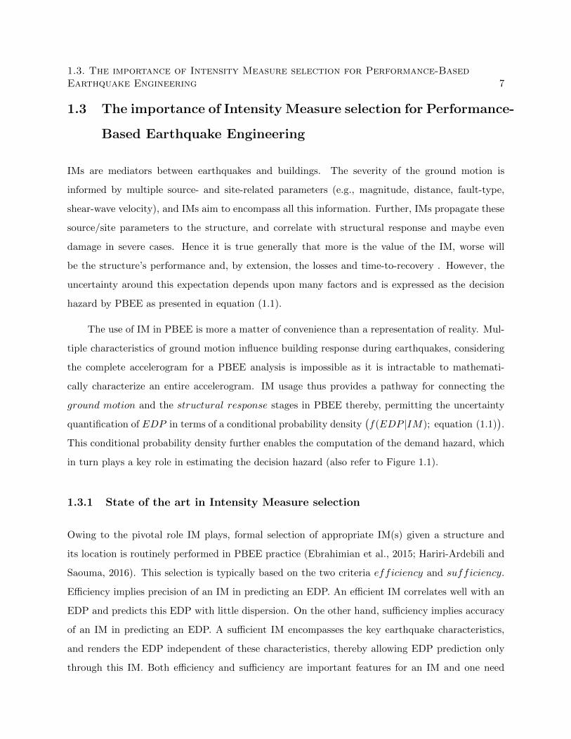
Owing to the pivotal role IM plays, formal selection of appropriate IM(s) given a structure and
its location is routinely performed in PBEE practice (Ebrahimian et al., 2015; Hariri-Ardebili and
Saouma, 2016). This selection is typically based on the two criteria efficiency and sufficiency.
Efficiency implies precision of an IM in predicting an EDP. An efficient IM correlates well with an
EDP and predicts this EDP with little dispersion. On the other hand, sufficiency implies accuracy
of an IM in predicting an EDP. A sufficient IM encompasses the key earthquake characteristics,
and renders the EDP independent of these characteristics, thereby allowing EDP prediction only
through this IM. Both efficiency and sufficiency are important features for an IM and one need
8 Chapter 1. Introduction
not imply the other; a schematic of this is portrayed in Figure 1.3. Practically speaking, while
IM efficiency is evaluated by computing the (log) standard deviation in EDP given this IM (i.e.,
the dispersion), sufficiency is evaluated by performing null hypothesis tests (i.e., by computing
p-values) concerning multiple earthquake parameters such as magnitude, distance, fault-type, etc.
It is noted that efficiency evaluation is quantitative, and sufficiency evaluation is qualitative and
has multiple criteria owing to the several p-values across earthquake parameters.
(a) (b)
Figure 1.3: Demonstration of the concepts of IM efficiency and sufficiency. (a) An efficient, butnot sufficient, IM may lead to precise (i.e., less dispersed) PBEE results but there is no guaranteethat these results are accurate. (b) A sufficient, but not efficient, IM may lead to accurate PBEEresults, but with more dispersion. In summary, both efficiency and sufficiency are complementingattributes for an IM.
1.3.2 Need for quantitative methods for Intensity Measure selection
PBEE is built on the premise of quantitativeness in its analysis stages. The criteria for IM selection
as a whole, however, can be described as semi-quantitative at the most: quantitative efficiency
and qualitative sufficiency concerning the multiple earthquake parameters. This lack of a single,
quantitative criteria is an impediment towards selecting the best IM. Many studies in literature
compute the standard deviation in EDP given IM (efficiency) and the pass/fail p-values concerning
the multiple earthquake parameters yet do not have any concrete conclusions about the relative
suitability of various IMs (for e.g. see Hariri-Ardebili and Saouma 2016; Luco and Cornell 2007;
Padgett et al. 2008; Shakib and Jahangiri 2016). Thus, a single metric that quantifies an IM’s overall

1.4. Ground motion selection for Performance-Based Earthquake Engineering 9
quality concerning both efficiency and sufficiency is desirable to not only identify with certainty
the best IM, but also understand how the alternatives fare with respect to the ‘best.’ Such an
understanding has the potential for allowing PBEE to more completely characterize the ground
motion as opposed to relying on a single IM. More discussion on this aspect will be presented
towards the end of this thesis.
1.4 Ground motion selection for Performance-Based Earthquake
Engineering
Ground motion record selection is required to estimate the uncertainty in EDP given an IM level
through the conditional density function(f(EDP |IM)
). Similar to IM selection, the nature of
the record set selected is shown to have a significant influence on the demand hazard and, by
extension, the decision hazard. Methods for selecting appropriate ground motions that not only
are consistent with the seismic hazard at a site, but also produce reliable estimates of building
response uncertainty have been a topic of considerable interest.
1.4.1 State-of-the-art in ground motion selection
Methods for selecting ground motions in PBEE are varied—and often dependent on the ana-
lyst—unlike IM selection where analysts mostly rely on criteria such as efficiency and sufficiency.
These methods can be broadly divided into two categories: (i) selecting ground motions that meet
specific criteria; (ii) hazard consistent ground motion selection. In the first category, ground motions
that have specific ranges of earthquake parameters such as magnitude and distance are selected to
populate the record set. The Federal Emergency Management Authority document P695 far-field
record set and the Medina-Krawinkler large magnitude small distance record set are some popular
examples (FEMA P695, 2009; Medina, 2003). In the second category, a target response spectrum
that considers information about the site hazard is used for ground motion selection, and often,
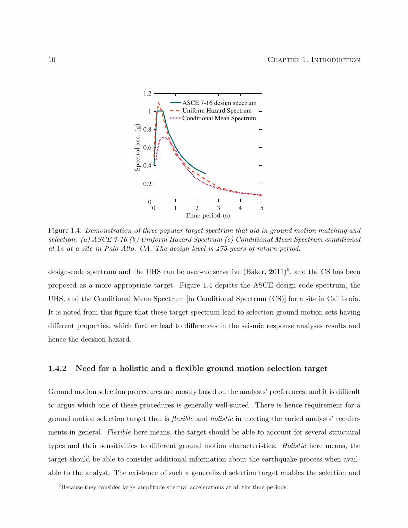
amplitude scaling of recorded accelerograms to match this target spectrum is performed. Popular
targets include the design-code spectrum (ASCE7, 2010), the Uniform Hazard Spectrum (Baker,
2008), and the more recent Conditional Spectrum (Lin et al., 2013b). It has been argued that the
10 Chapter 1. Introduction
0 1 2 3 4 5Time period (s)
0
0.2
0.4
0.6
0.8
1
1.2
Spectralacc.(g)
ASCE 7-16 design spectrum
Uniform Hazard Spectrum
Conditional Mean Spectrum
Figure 1.4: Demonstration of three popular target spectrum that aid in ground motion matching andselection: (a) ASCE 7-16 (b) Uniform Hazard Spectrum (c) Conditional Mean Spectrum conditionedat 1s at a site in Palo Alto, CA. The design level is 475-years of return period.
design-code spectrum and the UHS can be over-conservative (Baker, 2011)5, and the CS has been
proposed as a more appropriate target. Figure 1.4 depicts the ASCE design code spectrum, the
UHS, and the Conditional Mean Spectrum [in Conditional Spectrum (CS)] for a site in California.
It is noted from this figure that these target spectrum lead to selection ground motion sets having
different properties, which further lead to differences in the seismic response analyses results and
hence the decision hazard.
1.4.2 Need for a holistic and a flexible ground motion selection target
Ground motion selection procedures are mostly based on the analysts’ preferences, and it is difficult
to argue which one of these procedures is generally well-suited. There is hence requirement for a
ground motion selection target that is flexible and holistic in meeting the varied analysts’ require-
ments in general. Flexible here means, the target should be able to account for several structural
types and their sensitivities to different ground motion characteristics. Holistic here means, the
target should be able to consider additional information about the earthquake process when avail-
able to the analyst. The existence of such a generalized selection target enables the selection and
5Because they consider large amplitude spectral accelerations at all the time periods.
1.5. Research objectives 11
use of those ground motions to which the analyst thinks the building would be vulnerable against
damage and/or collapse. This further, through the PBEE uncertainty propagation framework, will
introduce more confidence in the estimates of decision hazard, and this confidence also reflects on
the building performance.
It is noted that the development of a generalized method for computing the target spectrum
needs to be supported by a more complex seismic hazard analysis that focuses on multiple IMs rather
than a single IM. This is because, if a structural type is sensitive to multiple IMs, ground motions
that represent the desired hazard levels concerning these multiple IMs are essentially selected. The
IM values that correspond to these hazard levels are identified through vector Probabilistic Seismic
Hazard Analysis (PSHA). Vector PSHA has been of considerable interest to the PBEE community,
although, almost all of the PSHA software available are only equipped to treat scalar IMs. There-
fore, there is a necessity to develop a simple procedure for performing vector PSHA that relies on
the scalar outputs of a PSHA software, but is also consistent with the modern PSHA standards.
Such consistency is important because modern PSHA considers many complexities related to the
seismic activity at a particular site with the aim of presenting an accurate representation of the
hazard.
1.5 Research objectives
The over-arching goal of this thesis is to develop methods and tools that enable improved IM
and ground motion selection for PBEE analysis. In doing so, the change of perspective, and the
mechanism to incorporate additional information provided by Bayesian methods will be utilized.
There are three specific research objectives:
O1: A unified metric for Intensity Measure quality assessment
IM sufficiency has been evaluated qualitatively through p-values causing impediments to prop-
erly selecting IMs. A quantitative metric for IM sufficiency that evaluates the degree of indepen-
dence of an EDP from all the earthquake parameters considered is proposed using Bayes rule and
Information Theory. Performance evaluation of the proposed metric is made by verifying if the
this metric gauges bias in demand hazard curves due to the inclusion of earthquake parameters.
12 Chapter 1. Introduction
Then, with the aim of proposing a unified metric for assessing IM quality, this metric is combined
with the metric for efficiency by understanding the relationship between these two criterion for IM
selection.
O2: A pre-configured solution to the problem of vector seismic hazard analysis
An efficient and an accurate Bayesian method for vector Probabilistic Seismic Hazard Analysis
(PSHA) is proposed, which relies on outputs from scalar PSHA software, and avoids the repetition
of expensive hazard computations. The solution should only utilize the basic outputs available
from most PSHA software: scalar hazard curves and M-R deaggregation matrices. Additionally,
the solution should be consistent with modern PSHA standards, accounting for the fault-specific
parameters of the multiple fault-sources considered and the logic-tree. The development of this
simplified method for vector PSHA is in support of the ground motion selection target next dis-
cussed.
O3: A Bayesian Conditional Spectrum approach for holistic and flexible ground motion
selection
A holistic and flexible ground motion selection target is developed by adopting a Bayesian
approach. This generalized method for computing the target spectrum is termed as the Bayesian
CS and it offers the following advantages in terms of being holistic and flexible: (i) Consideration
of multiple causal events that can result in the same ground motion IM level; (ii) Incorporation
of additional information about the earthquake process through the prior distributions; and (iii)
Extending the CS to a general class of structures that are sensitive to different characteristics of
the ground motion beyond Sa.
1.6 Organization
This thesis is organized into the following six chapters:
Chapter 2 will cover background surrounding seismic hazard analysis, IM selection, and ground
motion selection. The application of Bayesian methods in PBEE will also be discussed.

1.6. Organization 13
Chapter 3 will demonstrate the application of Bayesian methods in PBEE and will contrast them
with Frequentist methods. The problem of capturing heteroscedasticity in structural seismic
response analyses will be used as an example.
Chapter 4 will propose a Bayesian quantitative metric for sufficiency of IMs and then will investi-
gate the relationship between the efficiency and the sufficiency metrics. Much of this chapter
will be based on a journal publication with some additions concerning the unified metric for
sufficiency and efficiency.
Chapter 5 will propose a Bayesian-driven simplified method for vector seismic hazard analysis.
Much of this chapter will be based on a journal publication.
Chapter 6 will develop a Bayesian methodology for the CS to aid ground motion selection. Much
of this chapter will be based on a journal publication ready for submission.
Chapter 7 will discuss this thesis’ summary, conclusions, and future work.
This thesis has resulted in (or will result in) the following publications:
1. Somayajulu L.N. Dhulipala, Adrian Rodriguez-Marek, Shyam Ranganathan, and Madeleine
M. Flint. “A site-consistent method to quantify suciency of alternative IMs in relation to
PSDA.” Earthquake Engineering & Structural Dynamics 47(2) 2018: 377-396.
2. Somayajulu L.N. Dhulipala, Adrian Rodriguez-Marek, and Madeleine M. Flint. “Compu-
tation of vector hazard using salient features of seismic hazard deaggregation” Earthquake
Spectra 34(4) 2018: 1893-1912.
3. Somayajulu L.N. Dhulipala and Madeleine M. Flint. “Bayesian Conditional Spectrum for
Ground Motion Selection” Earthquake Engineering & Structural Dynamics (under review).
4. Somayajulu L.N. Dhulipala and Madeleine M. Flint. “Use of Generalized Linear Models to
capture seismic response heteroscedasticity of four-story steel moment frame building” In
proceedings of 12th Int. Conf. on Structural Safety and Reliability (ICOSSAR): 711-720.
2017. Vienna, Austria.
Chapter 2
Background
This chapter provides a background on Intensity Measure and ground motion selection methods in
Performance-Based Earthquake Engineering (PBEE). Additionally, a primer on Bayesian statistical
methods is provided.
2.1 State of Research in Intensity Measure Selection
As noted in Chapter 1, several Intensity Measures (IM) can be derived from an earthquake record
and it is important to select that IM which ensures an accurate and a precise probabilistic represen-
tation of the structural seismic performance. Criterion such as efficiency, sufficiency, proficiency,
and hazard computability have been therefore proposed to aid the selection of alternative IMs.
These criterion are discussed in this section.
2.1.1 Efficiency
Efficiency measures how well an IM correlates with an EDP. Shome (1999) is perhaps the first to
propose the efficiency criterion to aid the selection of an appropriate IM. Since then, this criterion
has been applied to a variety of structures, geo-structures, and infrastructure systems. Numerous
studies conclude that spectral acceleration at the first-mode period of the structure(Sa(T1)
)tends
to be an efficient IM for drift related EDPs of short to medium height buildings (Freddi et al., 2016;
Giovenale et al., 2004; Luco and Cornell, 2007). Kohrangi et al. (2017) propose that spectral accel-
eration averaged across multiple periods (Saavg) is generally efficient across drift, floor-acceleration,
and rotation related EDPs of buildings. Concerning a portfolio of bridges, Padgett et al. (2008)
find that Peak Ground Acceleration (PGA) and Saavg are both equally efficient. For a structure
14
2.1. State of Research in Intensity Measure Selection 15
supported on pile foundations, Bradley et al. (2009) find that Cumulative Absolute Velocity is
an efficient IM. Shakib and Jahangiri (2016) find that Velocity Spectrum Intensity is a generally
efficient IM for buried pipelines. The concept of efficiency has been extended to vector-valued IMs
by Baker and Cornell (2005). Vector-valued IMs are a combination of two or more IMs, and Baker
and Cornell (2005) find that a combination of Sa(T1) and ε1 tends to be more efficient than only
Sa(T1) for first mode dominated structures.
In a cloud-based analysis, EDP and IM are related through a regression model. Mathematically
then, efficiency is defined as the standard deviation in predicting an EDP with IM as the predictor
variable (Luco and Cornell, 2007). Consider the following generic regression model between EDP
and IM:
log(EDP ) = F(
log(IM))
+ e (2.1)
where F (.) is the functional form used for predicting EDP as a function of IM and e is the residual.
Standard deviation of the above prediction or IM efficiency is defined as:
βEDP |IM =
√√√√∑Ni=1
[log(EDPi)− F
(log(IMi)
)]N − 2
(2.2)
where N indicates the number of EDP-IM pairs in the seismic response analyses and i indicates
the index of a particular pair. A depiction of efficiency is provided in Figure 2.1a. It is observed
that lower the value of βEDP |IM , better is the efficiency of an IM since it correlates well with an
EDP. It is common practice to use a simple linear model for F(
log(IM))
of the form (Giovenale
et al., 2004; Luco and Cornell, 2007):
F(
log(IMi))
= a+ b log(IMi) (2.3)
where a and b are the regression coefficients. However, studies such as Freddi et al. (2016) have
proposed a bilinear model, and Mangalathu et al. (2018) use machine learning techniques to predict
1ε is the normalized residual between the observed and the predicted value of an IM.
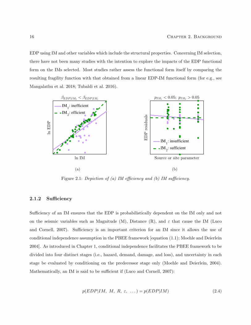
16 Chapter 2. Background
EDP using IM and other variables which include the structural properties. Concerning IM selection,
there have not been many studies with the intention to explore the impacts of the EDP functional
form on the IMs selected. Most studies rather assess the functional form itself by comparing the
resulting fragility function with that obtained from a linear EDP-IM functional form (for e.g., see
Mangalathu et al. 2018; Tubaldi et al. 2016).
ln IM
lnEDP
βEDP |IM2< βEDP |IM1
IM1: inefficient
IM2: efficient
(a)
Source or site parameter
EDPresiduals
pIM1< 0.05; pIM2
> 0.05
IM1: insufficient
IM2: sufficient
(b)
Figure 2.1: Depiction of (a) IM efficiency and (b) IM sufficiency.
2.1.2 Sufficiency
Sufficiency of an IM ensures that the EDP is probabilistically dependent on the IM only and not
on the seismic variables such as Magnitude (M), Distance (R), and ε that cause the IM (Luco
and Cornell, 2007). Sufficiency is an important criterion for an IM since it allows the use of
conditional independence assumption in the PBEE framework [equation (1.1); Moehle and Deierlein
2004]. As introduced in Chapter 1, conditional independence facilitates the PBEE framework to be
divided into four distinct stages (i.e., hazard, demand, damage, and loss), and uncertainty in each
stage be evaluated by conditioning on the predecessor stage only (Moehle and Deierlein, 2004).
Mathematically, an IM is said to be sufficient if (Luco and Cornell, 2007):
p(EDP |IM, M, R, ε, . . . ) = p(EDP |IM) (2.4)
2.1. State of Research in Intensity Measure Selection 17
where it is seen that the EDP is conditionally independent of the various source or site parameters
in the seismic hazard analysis (M, R, ε, . . . ). Sufficiency is traditionally evaluated by computing
p-values (Luco and Cornell, 2007), where the EDP residuals are first computed using log(IMi) −
F(
log(IMi)). Next, a null hypothesis test is conducted on these EDP residuals with respect to
one of the source or site parameters. If the resulting p-value is greater than a significance level,
the IM is independent of this source or site parameter, and otherwise, it is not. This procedure is
repeated multiple times with different source or site parameter and IM sufficiency with respect to
these parameters is ascertained.
Figure 2.1b presents an illustration of IM sufficiency, where it is noted that IM1, having a p-
value less than the significance level 0.05, is insufficient; whereas, IM2 is sufficient. Consequently,
we see bias in EDP residuals with respect to a source or site parameter when IM1 is used, and
when IM2 is used, this bias is absent. It is customary to fix the significance level as 0.05, although
Padgett et al. (2008) use a value of 0.10. This procedure for evaluating IM sufficiency has been
applied in numerous studies concerning the seismic analysis of infrastructure (Bradley et al., 2009;
Freddi et al., 2016; Hariri-Ardebili and Saouma, 2016); however, as will be seen in Chapter 4, the
procedure for evaluating IM sufficiency is qualitative and suffers from having multiple criterion
which make ascertaining the most sufficient IM among a suite of IMs quite difficult. Jalayer
et al. (2012) propose an alternative evaluation procedure of IM sufficiency using principles from
Information Theory. This metric, however, defines sufficiency as the ground motion representation
ability of an IM, rather than conditional independence (see Appendix A).
2.1.3 Hazard Computability
Many advanced IMs are being proposed that are more efficient and sufficient than traditional IMs
such as Sa(T1) and PGA. Marafi et al. (2016) is an example study that proposes a new IM to
capture the intensity as well as spectral shape and duration of an earthquake. Given the frequent
proposal of new IMs to suit the specific application and structural type, it is important that these
IMs have their seismic hazard curves available in order to facilitate a PBEE analysis using equation
(1.1). Hazard computability is therefore introduced as a criterion for selecting alternative IMs by
Giovenale et al. (2004). Many efforts have gone into developing the hazard curves for new/advanced
18 Chapter 2. Background
IMs by first developing Ground Motion Prediction Models (GMPM) for these IMs. For example,
Kohrangi et al. (2018) and Kale et al. (2017) develop GMPMs for Saavg and fractional order IMs,
respectively, to facilitate their use in PBEE.
2.2 State of Research in Ground Motion Selection Tools
Ground motion selection is an important aspect of PBEE, and the nature of ground motions se-
lected for structural response analysis can significantly influence demand hazard phase in PBEE
(Baker and Cornell, 2006). While ground motions can be qualitatively selected by specifying ranges
of magnitude, distance, and PGA amplitude(e.g., FEMA P695 (2009)
), the focus in this thesis is
upon tools which use target spectrum matching or distribution matching for automatically select-
ing ground motions. Three such tools will be discussed here: Uniform Hazard Spectrum (UHS),
Conditional Mean Spectrum (CMS), and Generalized Conditioning Intensity Measure (GCIM).
2.2.1 Seismic Hazard Analysis and Uniform Hazard Spectrum
UHS is popular target spectrum that is prescribed by design codes (ASCE, 2016) and is also used
for the seismic vulnerability assessment of buildings, nuclear plants, and other structures (Ali et al.,
2014; Goulet et al., 2007) in research. Typically, given a UHS (refer to Figure 1.4), those ground
motions whose spectral ordinates match with the UHS are selected. The sum of squares of errors is
generally used as a metric to assess the degree of matching and ground motions are usually scaled
in the matching process (Bradley, 2012c).
To understand how an UHS is constructed, an overview of Probabilistic Seismic Hazard Anal-
ysis (PSHA) is presented; however, it is noted that (Baker, 2008) provides a more thorough intro-
duction to PSHA. PSHA computes the annual frequency of exceedance of an IM(λ(IM > x)
)by
accounting for all possible magnitude and distance combinations (M, R) that can result in the IM
value while considering all the seismic sources near a site. A PSHA is represented by the following
equation which is an application of the total probability theorem (Lin, 2012):

2.2. State of Research in Ground Motion Selection Tools 19
λ(IM > x) =∑Ns
∫M
∫RP (IM > x|M,R) f(M) f(R) dM dR (2.5)
where Ns is the number of seismic source, P (IM > x|M,R) is the conditional probability of
exceeding an IM value given (M,R), and f(M) and f(R) are the probability densities of equalling
M and R, respectively. A schematic of PSHA is provided in Figure 2.2a. The f(M) and f(R)
distributions for a seismic source are computed from recorded data of magnitudes and hypocenter
locations, respectively.2 The conditional probability P (IM > x|M,R) is computed through a
GMPM, particularly by analyzing the residuals of a GMPM and fitting a probability distribution
to these residuals.
# e
arth
qu
ake
> m
Magnitude, m
Distance, R Ground motion IM
Haz
ard
Gro
un
d m
oti
on
IM
Source 1
Source 2
Step 1: Identify
seismic sources
Step 2: Characterize each source
with a recurrence function
Step 3: Estimate the
median ground motion
Step 4: Integrate ground motion
uncertainty from all sources
(a)
Sa(0.3s) (g)
Haz
ard
Sa(1s) (g)
Haz
ard
(b)
Figure 2.2: (a) Illustration of PSHA. (b) Illustration of computing the UHS using PSHA results.
The UHS is computed through PSHA results. First, the design hazard level is selected; for
example, the 2475-year return period; that is, the Maximum Considered Earthquake level. Then for
a suite of spectral periods, PSHA is performed for a site and the spectral acceleration value for each
period corresponding to the target hazard level is plotted against the time period on the x-axis. The
2Instead of using hypocenter data for estimating the distance uncertainty, it is many times assumed that alllocations on the fault are equally likely to rupture, leading to an exponential distribution for f(R).
20 Chapter 2. Background
resulting response spectrum is the UHS and Figure 2.3 provides an illustration of deriving the UHS
from PSHA results. Although the UHS is a popular target spectrum for ground motion selection, it
has been criticized for its overconservativeness in portraying the structural performance (Baker and
Cornell, 2006; Koopaee et al., 2017). The reason for this overconservatism is, the UHS represents
multiple large earthquake events since spectral accelerations at multiple periods are conditioned
on amplitudes corresponding to the same hazard level. In reality, however, a structure will be
subjected to only one of those earthquake events at a given time. The consideration of multiple
earthquake events by the UHS therefore overestimates the future ground motion potential.
2.2.2 Conditional Mean Spectrum
Overconservatism of the UHS can be remedied by using the Conditional Mean Spectrum (CMS).
Rather than relying on multiple large earthquake events, the CMS relies on a single such event.
The spectral acceleration amplitude at a desired period (typically the fundamental mode period of
the structure) is specified, and the CMS is computed through (Baker, 2011):
µSa(Ti)|Sa(T1) = µSa(Ti) + σSa(Ti) ρSa(Ti),Sa(T1)Sa(T1)− µSa(Ti)
σSa(T1)(2.6)
where µ. is the predicted value of spectral acceleration from a GMPM, σ. is the GMPM standard
deviation, ρ., . is the correlation coefficient between two spectral periods (for e.g., computed from
Baker and Jayaram 2008), and Sa(T1) is the specified value of spectral acceleration at a desired
time period obtained using PSHA results. Baker (2011) noted that it also essential to account for
the variability around the CMS as a result of the variability of GMPMs. Consequelty, Baker (2011)
proposed the target variability as:
σSa(Ti)|Sa(T1) = σSa(Ti)
√1− ρ2Sa(Ti),Sa(T1) (2.7)
A pictorial depiction of the CMS and the matched ground motions which obey the target variability
around the CMS is presented in Figure 2.3a. Lin et al. (2013b) term the CMS and the variability
around it as the Conditional Spectrum (CS), and further note that CS-matched ground motions
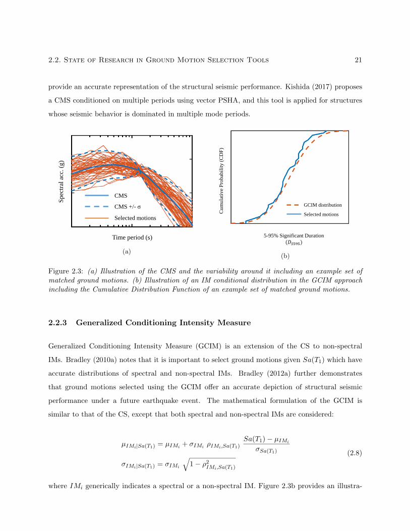
2.2. State of Research in Ground Motion Selection Tools 21
provide an accurate representation of the structural seismic performance. Kishida (2017) proposes
a CMS conditioned on multiple periods using vector PSHA, and this tool is applied for structures
whose seismic behavior is dominated in multiple mode periods.
Time period (s)
Sp
ectr
al a
cc.
(g)
CMS
CMS +/- σ
Selected motions
(a)
5-95% Significant Duration
(𝐷𝑆595)
Cu
mu
lati
ve
Pro
bab
ilit
y (
CD
F)
GCIM distribution
Selected motions
(b)
Figure 2.3: (a) Illustration of the CMS and the variability around it including an example set ofmatched ground motions. (b) Illustration of an IM conditional distribution in the GCIM approachincluding the Cumulative Distribution Function of an example set of matched ground motions.
2.2.3 Generalized Conditioning Intensity Measure
Generalized Conditioning Intensity Measure (GCIM) is an extension of the CS to non-spectral
IMs. Bradley (2010a) notes that it is important to select ground motions given Sa(T1) which have
accurate distributions of spectral and non-spectral IMs. Bradley (2012a) further demonstrates
that ground motions selected using the GCIM offer an accurate depiction of structural seismic
performance under a future earthquake event. The mathematical formulation of the GCIM is
similar to that of the CS, except that both spectral and non-spectral IMs are considered:
µIMi|Sa(T1) = µIMi + σIMi ρIMi,Sa(T1)Sa(T1)− µIMi
σSa(T1)
σIMi|Sa(T1) = σIMi
√1− ρ2IMi,Sa(T1)
(2.8)
where IMi generically indicates a spectral or a non-spectral IM. Figure 2.3b provides an illustra-
22 Chapter 2. Background
tion of a conditional distribution of an IM given the conditioning IM Sa(T1) and the Cumulative
Distribution Function of an example set of matched ground motions.
2.3 Bayesian Methods: A Primer
Bayesian methods will be used in this thesis to facilitate efficient IM selection and ground motion
selection in PBEE. As will be seen later chapters, the change of perspective, the flexibility to
incorporate new information, and the comprehensiveness in uncertainty quantification offered by
Bayesian methods are used to solve some key problems related to IM and ground motion selection.
A brief background on Bayesian methods is presented here. The important concepts in Bayesian
analysis covered here are a synthesis of the material presented in Hoff (2009).
The following notations will be frequently used: P (.) Probability, P (.|.) Conditional probabil-
ity, P (., .) Joint probability, f(.) Probability density, f(.|.) Conditional probability density, and
f(., .) Joint probability density.
2.3.1 Bayes rule
For the case of discrete events, the Bayes rule is given by:
P (A|B) =P (B|A) P (A)
P (B|A)P (A) + P (B|A)P (A)(2.9)
where A and B denote events and (.) denotes the complement of an event. In equation (2.10),
P (A|B) denotes the conditional probability of event A happening given B [P (B|A) can be inter-
preted similarly] and P (A) denotes the marginal probability of event A [P (B) can be interpreted
similarly]. In Bayesian language, P (A) is termed the prior probability and P (A|B) is termed the
posterior probability. The reasoning behind this nomenclature is that, P (A) represents the proba-
bility of event A occurring before the knowledge of event B, P (A|B) represents the probability of
event A occurring after the knowledge of event B. A continuous analog of Bayes rule is:
2.3. Bayesian Methods: A Primer 23
fY (y|X = x) =fX(x|Y = y) fY (y)∫
Y fX(x|Y = y) fY (y) dy(Full notation)
f(y|x) =f(x|y) f(y)∫
Y f(x|y) f(y) dy(Shorthand notation)
(2.10)
where X, Y are continuous random variables representing real life events or phenomenon, and x,
y are the specific values X, Y take. While the first line in equation (2.10) is an accurate way to
represent Bayes rule for continuous random variables, the second line uses a shorthand notation
that omits the specific random variable in the subscript. This shorthand notation will be used
throughout this thesis. In Bayesian language, f(y) is termed the prior distribution and f(y|x) is
termed the posterior distribution since these represent possibilities of different values of Y before
and after observing X = x, respectively. The distribution f(x|y) is referred to as a likelihood
function.
Multiple random variables: Often times in practice, it is necessary to estimate the joint
posterior distribution of multiple random variables given multiple random variables; for example,
f(p, q|x, y). In such cases, Bayes rule takes the form:
f(p, q|x, y) =f(x, y|p, q) f(p, q)∫
P
∫Q f(x, y|p, q) f(p, q) dp dq
(2.11)
where f(p, q) represents a joint prior distribution over P,Q and the denominator represents the
total probability density f(x, y).
Multiple observations of random variables: Also necessary in practice is Bayesian analy-
sis of a random variable with N observations. For example, if P,Q are the random variables whose
posterior distributions are to be inferred given multiple values of the random variable X, Bayes
rule takes the form:
f(p, q|x) =
∏Ni=1 f(xi|p, q) f(p, q)∫
P
∫Q
∏Ni=1 f(xi|p, q) f(p, q) dp dq
(2.12)
24 Chapter 2. Background
where x is the vector of observed values of X and i is the index. Notice the product operation over
the likelihoods of individual xi observations. This implies that the observations in x are indepen-
dent and identically distributed (IID). Independent because they have been observed without any
connection to each other, and identically distributed because these observations follow the same
probability distribution (say a Gaussian). IID is an important condition in Bayesian analysis which
is encountered or frequently assumed in practice.
2.3.2 Prior distributions, Conjugate priors, and Non-informative priors
Prior distributions (or simply “priors”) constitute one important aspect that separates Bayesian
from Frequentist. Some argue that priors are poorly defined in Bayesian theory and that they
introduce subjectivity in the analysis. While many others see priors as an opportunity to learn
more from given data, to design models to suit analysts’ requirements, and more importantly,
to leverage the adaptability of the Bayesian procedure for solving many practical problems. For
example, consider the following problem concerning rapid earthquake damage estimation.
A county is located near an active subduction zone and is subjected to a magnitude 7 earth-
quake. Local authorities wanted to quickly estimate the probability of severe damage (P ) to the
whole county so as to assess the required mitigation efforts. They rely on “Did you feel it?” data
to get responses from the N = 20 citizens who reported whether or not their homes sustained
severe damages. Only relying on this data, the authorities compute probability of severe damage
using: 1/N∑N
i=1 Yi (Yi is 1 if ith citizen’s home sustained severe damage and 0 otherwise). The
probability P turns out to be 0.65. However, there are two significant caveats: (i) the sample size
N is not large enough; (ii) citizens’ assessment of damage to their homes can be biased.
Fortunately, the authorities have historical data concerning earthquake damage from around
the world through which they estimate that the probability of severe damage at a regional scale is
Beta distributed with parameters (α1 = 15, α2 = 2). “Did you feel it?” data, being binary, can be
modeled using a binomial distribution. Bayesian analysis elegantly combines these two sources of
information in order to overcome the limitations of using “Did you feel it?” data only. Posterior
estimation of P is set up using:
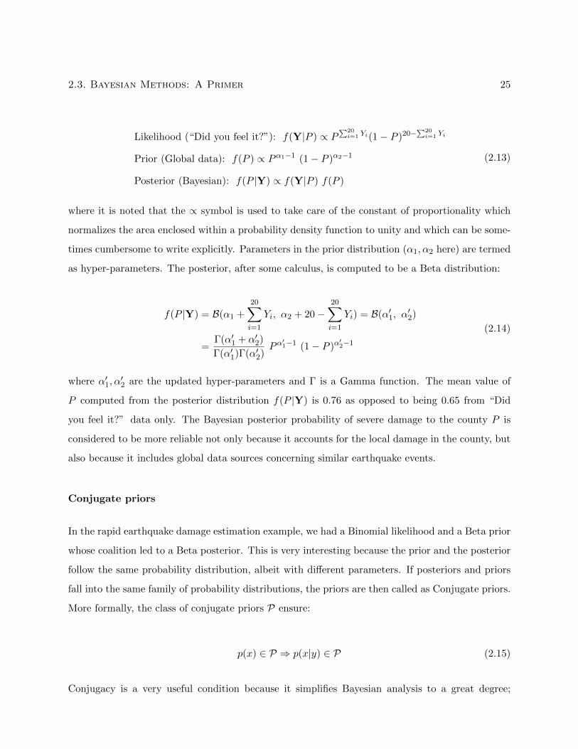
2.3. Bayesian Methods: A Primer 25
Likelihood (“Did you feel it?”): f(Y|P ) ∝ P∑20i=1 Yi(1− P )20−
∑20i=1 Yi
Prior (Global data): f(P ) ∝ Pα1−1 (1− P )α2−1
Posterior (Bayesian): f(P |Y) ∝ f(Y|P ) f(P )
(2.13)
where it is noted that the ∝ symbol is used to take care of the constant of proportionality which
normalizes the area enclosed within a probability density function to unity and which can be some-
times cumbersome to write explicitly. Parameters in the prior distribution (α1, α2 here) are termed
as hyper-parameters. The posterior, after some calculus, is computed to be a Beta distribution:
f(P |Y) = B(α1 +
20∑i=1
Yi, α2 + 20−20∑i=1
Yi) = B(α′1, α′2)
=Γ(α′1 + α′2)
Γ(α′1)Γ(α′2)Pα′1−1 (1− P )α
′2−1
(2.14)
where α′1, α′2 are the updated hyper-parameters and Γ is a Gamma function. The mean value of
P computed from the posterior distribution f(P |Y) is 0.76 as opposed to being 0.65 from “Did
you feel it?” data only. The Bayesian posterior probability of severe damage to the county P is
considered to be more reliable not only because it accounts for the local damage in the county, but
also because it includes global data sources concerning similar earthquake events.
Conjugate priors
In the rapid earthquake damage estimation example, we had a Binomial likelihood and a Beta prior
whose coalition led to a Beta posterior. This is very interesting because the prior and the posterior
follow the same probability distribution, albeit with different parameters. If posteriors and priors
fall into the same family of probability distributions, the priors are then called as Conjugate priors.
More formally, the class of conjugate priors P ensure:
p(x) ∈ P ⇒ p(x|y) ∈ P (2.15)
Conjugacy is a very useful condition because it simplifies Bayesian analysis to a great degree;
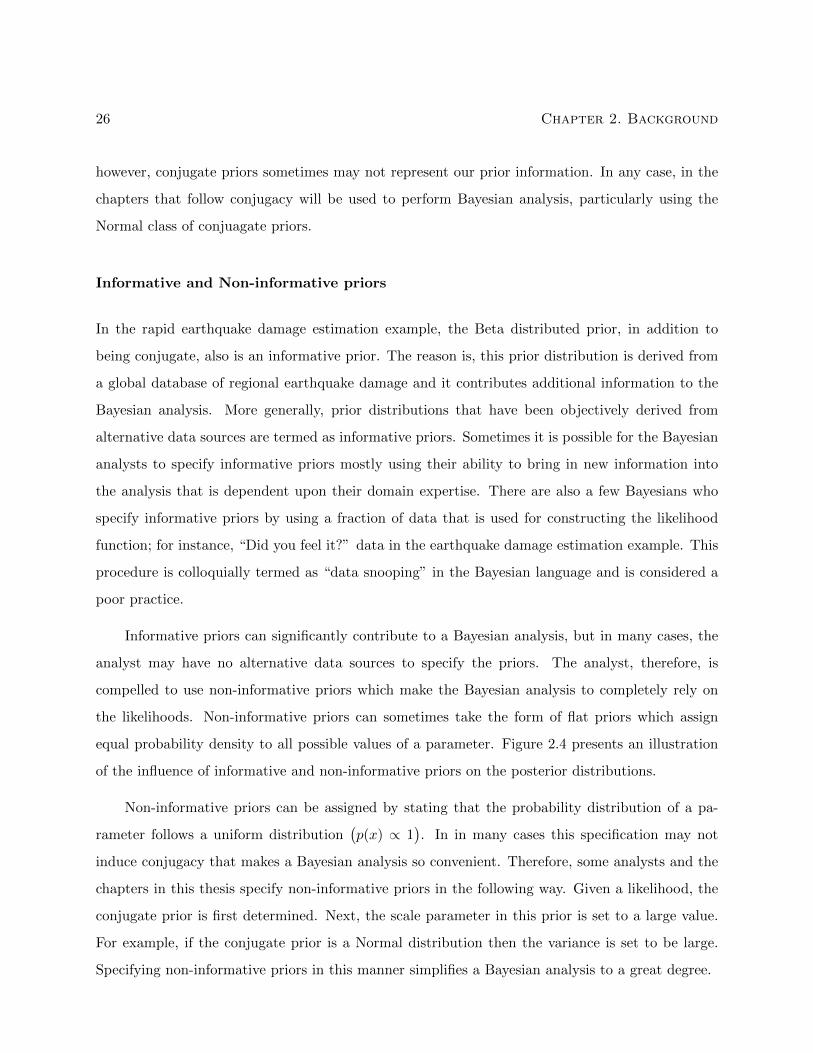
26 Chapter 2. Background
however, conjugate priors sometimes may not represent our prior information. In any case, in the
chapters that follow conjugacy will be used to perform Bayesian analysis, particularly using the
Normal class of conjuagate priors.
Informative and Non-informative priors
In the rapid earthquake damage estimation example, the Beta distributed prior, in addition to
being conjugate, also is an informative prior. The reason is, this prior distribution is derived from
a global database of regional earthquake damage and it contributes additional information to the
Bayesian analysis. More generally, prior distributions that have been objectively derived from
alternative data sources are termed as informative priors. Sometimes it is possible for the Bayesian
analysts to specify informative priors mostly using their ability to bring in new information into
the analysis that is dependent upon their domain expertise. There are also a few Bayesians who
specify informative priors by using a fraction of data that is used for constructing the likelihood
function; for instance, “Did you feel it?” data in the earthquake damage estimation example. This
procedure is colloquially termed as “data snooping” in the Bayesian language and is considered a
poor practice.
Informative priors can significantly contribute to a Bayesian analysis, but in many cases, the
analyst may have no alternative data sources to specify the priors. The analyst, therefore, is
compelled to use non-informative priors which make the Bayesian analysis to completely rely on
the likelihoods. Non-informative priors can sometimes take the form of flat priors which assign
equal probability density to all possible values of a parameter. Figure 2.4 presents an illustration
of the influence of informative and non-informative priors on the posterior distributions.
Non-informative priors can be assigned by stating that the probability distribution of a pa-
rameter follows a uniform distribution(p(x) ∝ 1
). In in many cases this specification may not
induce conjugacy that makes a Bayesian analysis so convenient. Therefore, some analysts and the
chapters in this thesis specify non-informative priors in the following way. Given a likelihood, the
conjugate prior is first determined. Next, the scale parameter in this prior is set to a large value.
For example, if the conjugate prior is a Normal distribution then the variance is set to be large.
Specifying non-informative priors in this manner simplifies a Bayesian analysis to a great degree.
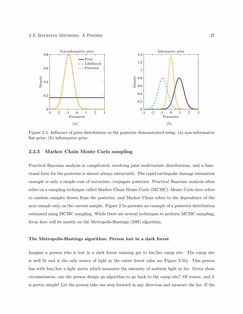
2.3. Bayesian Methods: A Primer 27
-3 -2 -1 0 1 2 3
Parameter
0
0.2
0.4
0.6
0.8
Density
Non-informative prior
Prior
Likelihood
Posterior
(a)
-3 -2 -1 0 1 2 3
Parameter
0
0.2
0.4
0.6
0.8
1
1.2
1.4
Density
Informative prior
(b)
Figure 2.4: Influence of prior distribution on the posterior demonstrated using: (a) non-informativeflat prior; (b) informative prior.
2.3.3 Markov Chain Monte Carlo sampling
Practical Bayesian analysis is complicated, involving joint multivariate distributions, and a func-
tional form for the posterior is almost always intractable. The rapid earthquake damage estimation
example is only a simple case of univariate, conjugate posterior. Practical Bayesian analysis often
relies on a sampling technique called Markov Chain Monte Carlo (MCMC). Monte Carlo here refers
to random samples drawn from the posterior, and Markov Chain refers to the dependence of the
next sample only on the current sample. Figure 2.5a presents an example of a posterior distribution
estimated using MCMC sampling. While there are several techniques to perform MCMC sampling,
focus here will be mostly on the Metropolis-Hastings (MH) algorithm.
The Metropolis-Hastings algorithm: Person lost in a dark forest
Imagine a person who is lost in a dark forest wanting get to his/her camp site. The camp site
is well lit and is the only source of light in the entire forest (also see Figure 2.5b). This person
has with him/her a light meter which measures the intensity of ambient light in lux. Given these
circumstances, can the person design an algorithm to go back to the camp site? Of course, and it
is pretty simple! Let the person take one step forward in any direction and measure the lux. If the
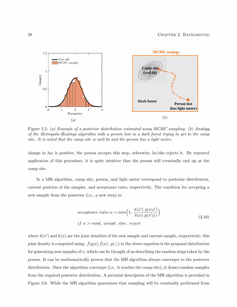
28 Chapter 2. Background
(a)
Camp site
(well lit)
Dark forest
MCMC analogy
Person lost
(has light meter)
(b)
Figure 2.5: (a) Example of a posterior distribution estimated using MCMC sampling. (b) Analogyof the Metropolis-Hastings algorithm with a person lost in a dark forest trying to get to the campsite. It is noted that the camp site is well lit and the person has a light meter.
change in lux is positive, the person accepts this step, otherwise, he/she rejects it. By repeated
application of this procedure, it is quite intuitive that the person will eventually end up at the
camp site.
In a MH algorithm, camp site, person, and light meter correspond to posterior distribution,
current position of the sampler, and acceptance ratio, respectively. The condition for accepting a
new sample from the posterior (i.e., a new step) is:
acceptance ratio α = min(
1,k(x′) g(x|x′)k(x) g(x′|x)
)if α > rand, accept; else, reject
(2.16)
where k(x′) and k(x) are the joint densities of the new sample and current sample, respectively; this
joint density is computed using: f(y|x) f(x). g(.|.) in the above equation is the proposal distribution
for generating new samples of x, which can be thought of as describing the random steps taken by the
person. It can be mathematically proven that the MH algorithm always converges to the posterior
distribution. Once the algorithm converges (i.e., it reaches the camp site), it draws random samples
from the required posterior distribution. A pictorial description of the MH algorithm is provided in
Figure 2.6. While the MH algorithm guarantees that sampling will be eventually performed from
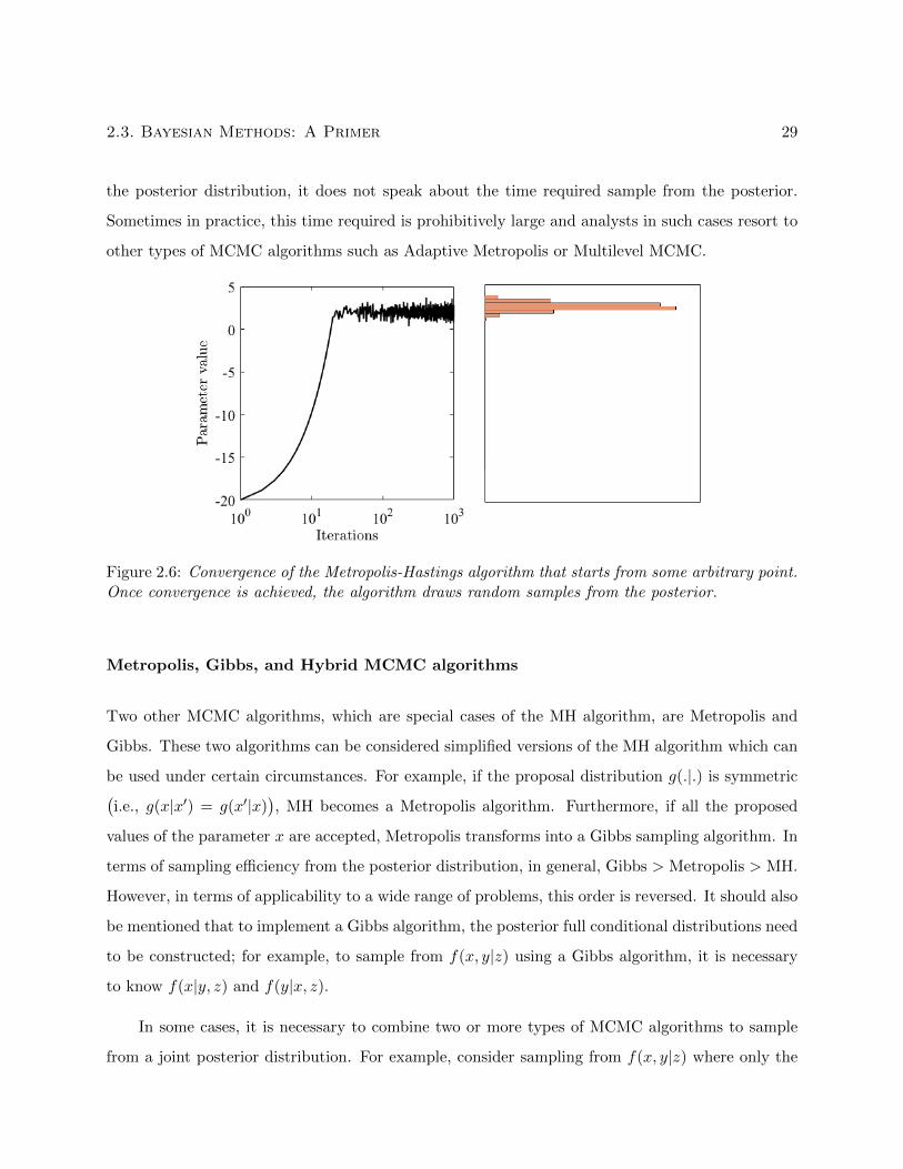
2.3. Bayesian Methods: A Primer 29
the posterior distribution, it does not speak about the time required sample from the posterior.
Sometimes in practice, this time required is prohibitively large and analysts in such cases resort to
other types of MCMC algorithms such as Adaptive Metropolis or Multilevel MCMC.
Figure 2.6: Convergence of the Metropolis-Hastings algorithm that starts from some arbitrary point.Once convergence is achieved, the algorithm draws random samples from the posterior.
Metropolis, Gibbs, and Hybrid MCMC algorithms
Two other MCMC algorithms, which are special cases of the MH algorithm, are Metropolis and
Gibbs. These two algorithms can be considered simplified versions of the MH algorithm which can
be used under certain circumstances. For example, if the proposal distribution g(.|.) is symmetric(i.e., g(x|x′) = g(x′|x)
), MH becomes a Metropolis algorithm. Furthermore, if all the proposed
values of the parameter x are accepted, Metropolis transforms into a Gibbs sampling algorithm. In
terms of sampling efficiency from the posterior distribution, in general, Gibbs > Metropolis > MH.
However, in terms of applicability to a wide range of problems, this order is reversed. It should also
be mentioned that to implement a Gibbs algorithm, the posterior full conditional distributions need
to be constructed; for example, to sample from f(x, y|z) using a Gibbs algorithm, it is necessary
to know f(x|y, z) and f(y|x, z).
In some cases, it is necessary to combine two or more types of MCMC algorithms to sample
from a joint posterior distribution. For example, consider sampling from f(x, y|z) where only the
30 Chapter 2. Background
posterior conditional f(x|y, z) is known. A direct utilization of the Gibbs algorithm is thus not
possible. However, within each iteration of the MCMC sampling, while Gibbs can be used to sample
from f(x|y, z), Metropolis or MH can be used to sample from f(y|x, z). There is mathematical
proof in Bayesian literature ensuring that this hybrid algorithm samples from the joint distribution
f(x, y|z). In chapter 3, a hybrid MCMC sampler is used to capture the heteroscedasticity in
structural seismic responses.
2.3.4 Information Theory in Bayesian Analysis
Information Theory is the study of loss/gain of information concerning evolving phenomenon. A
Bayesian analysis is considered to be evolving not only because the combination of likelihoods (or
new information) and priors (or old information) results in posteriors with updated information,
but also, different types of priors may lead to different posteriors and hence information content.
Information Theory is a vast subject area, and only two concepts in this broad field will be used
in this thesis. These concepts are Entropy and Relative Entropy described below, followed by an
example application in Bayesian analysis.
Entropy of the probability density f(x) is a measure of the missing information. Entropy in
f(x) is denoted by Sx and is mathematically defined as (Cover and Joy, 2012):
Sx = −∫xf(x) logn
(f(x)
)dx (2.17)
When the base of the logarithm is 2 (n = 2), entropy is measured in bits. Relative entropy (or
Kullback-Leibler divergence or information gain) between two densities f(x) and q(x) is a measure
of the difference between these density distributions. Relative entropy is denoted by DKL
(F ||Q
)and this notation indicates the amount of information gained by using the density f(x) in contrast
to the alternative density q(x). Mathematically, DKL
(F ||Q
)is defined as (Cover and Joy, 2012):
DKL
(F ||Q
)=
∫xf(x) logn
(f(x)
q(x)
)dx (2.18)
Again, if the base of the logarithm is 2, DKL
(F ||Q
)is measured in bits. It should be noted that
2.4. Summary 31
DKL
(F ||Q
)is always positive due to a condition called Jensen’s inequality.
Let us apply the Kullback-Leibler divergence to the non-informative/informative priors exam-
ple of Figure 2.4. The goal is to compare the amount of information gained through the posterior
density given non-informative (or uniform) and informative priors. DKL
(pos||pri
)computed using
uniform and informative priors turn out to be 1.53 and 2.61 bits, respectively. This implies that
informative priors provide 1.08 bits of additional information to the posterior estimation as com-
pared to non-informative priors. However, this statement must be taken with a grain of salt since a
poorly selected informative prior may lead to lesser information gain than a non-informative prior.
2.4 Summary
This chapter has reviewed relevant background on IM selection and ground motion selection is
PBEE, and also provided a primer on Bayesian statistical methods. The criterion which make an
IM optimal such as efficiency, sufficiency, proficiency, and hazard computability were discussed.
Different ground motion selection strategies that use one of the target spectra such as UHS, CMS,
or GCIM were mathematically discussed, in addition to providing some contrast between these
three spectra.
A considerable portion of this chapter dealt with providing basic background on Bayesian
methods. The different levels of complexity of the Bayes rule, the types of prior distributions
including informative and non-informative priors, and MCMC methods which enable a practical
implementation of Bayesian analysis were discussed. In addition, the entropy and the relative
entropy concepts in Information Theory, which support a Bayesian analysis, were also defined.
This background provided by this chapter is expected to support the later chapters in this thesis,
in terms of familiarzing the readers with concepts, principles, and techniques that will be employed.
Chapter 3
Application of Bayesian methods in
PBEE: Capturing heteroscedasticity
in seismic response analyses
This chapter is based on a study excerpted from:
Somayajulu L.N. Dhulipala and Madeleine M. Flint. “Use of Generalized Linear Models to capture
seismic response heteroscedasticity of four-story steel moment frame building” In proceedings of
12th Int. Conf. on Structural Safety and Reliability (ICOSSAR): 711-720. 2017. Vienna, Austria.
3.1 Introduction
The PEER framework for Performance Based Earthquake Engineering (PBEE) quantifies uncer-
tainty in decision variables (eg. cost) due to earthquakes by propagating uncertainties that exist at
various analysis levels, namely, seismic, demand, damage and loss analyses (Moehle and Deierlein,
2004). The crucial and computationally expensive stage of analysis in the PEER framework is
the estimation of demand hazard, which links earthquake occurrence intensity to structural dam-
age. The demand hazard computation stage is also termed Probabilistic Seismic Demand Analysis
(PSDA). One of the more straight-forward methods used in PSDA is the cloud-based approach
wherein structural response or Engineering Demand Parameters (EDP) from a suite of non-linear
dynamic analyses performed on the structure are linked to scalar earthquake Intensity Measures
(IM) using Ordinary Least Squares regression (OLS). Then, the probability that EDP exceeds a
particular value given IM is computed by assuming that OLS residuals are normally distributed.
This is shown as (Aslani and Miranda, 2005; Baker, 2007a; Freddi et al., 2016):
32
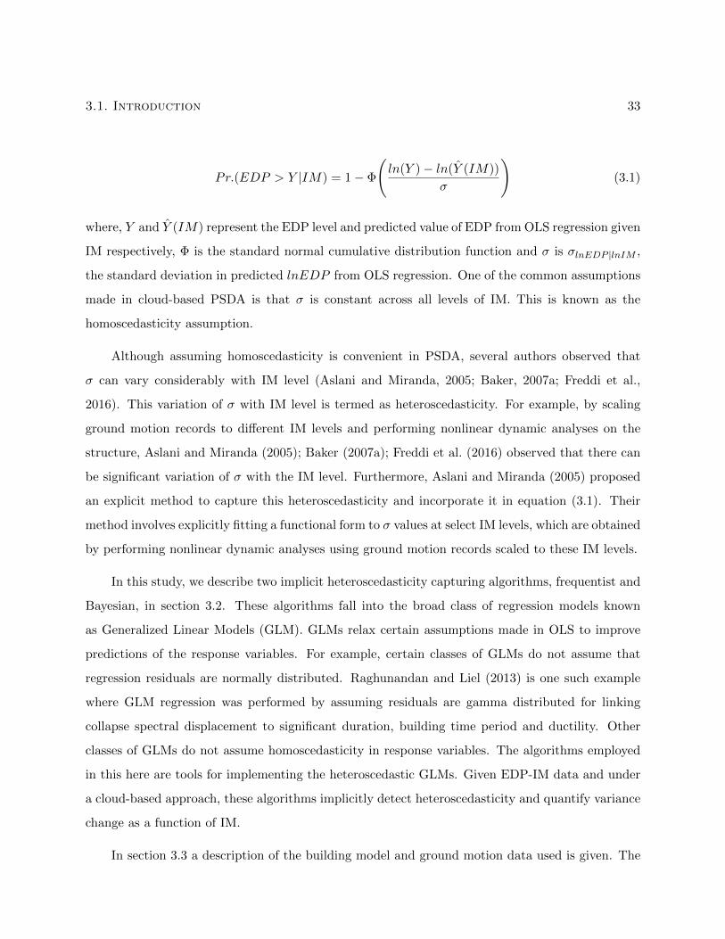
3.1. Introduction 33
Pr.(EDP > Y |IM) = 1− Φ
(ln(Y )− ln(Y (IM))
σ
)(3.1)
where, Y and Y (IM) represent the EDP level and predicted value of EDP from OLS regression given
IM respectively, Φ is the standard normal cumulative distribution function and σ is σlnEDP |lnIM ,
the standard deviation in predicted lnEDP from OLS regression. One of the common assumptions
made in cloud-based PSDA is that σ is constant across all levels of IM. This is known as the
homoscedasticity assumption.
Although assuming homoscedasticity is convenient in PSDA, several authors observed that
σ can vary considerably with IM level (Aslani and Miranda, 2005; Baker, 2007a; Freddi et al.,
2016). This variation of σ with IM level is termed as heteroscedasticity. For example, by scaling
ground motion records to different IM levels and performing nonlinear dynamic analyses on the
structure, Aslani and Miranda (2005); Baker (2007a); Freddi et al. (2016) observed that there can
be significant variation of σ with the IM level. Furthermore, Aslani and Miranda (2005) proposed
an explicit method to capture this heteroscedasticity and incorporate it in equation (3.1). Their
method involves explicitly fitting a functional form to σ values at select IM levels, which are obtained
by performing nonlinear dynamic analyses using ground motion records scaled to these IM levels.
In this study, we describe two implicit heteroscedasticity capturing algorithms, frequentist and
Bayesian, in section 3.2. These algorithms fall into the broad class of regression models known
as Generalized Linear Models (GLM). GLMs relax certain assumptions made in OLS to improve
predictions of the response variables. For example, certain classes of GLMs do not assume that
regression residuals are normally distributed. Raghunandan and Liel (2013) is one such example
where GLM regression was performed by assuming residuals are gamma distributed for linking
collapse spectral displacement to significant duration, building time period and ductility. Other
classes of GLMs do not assume homoscedasticity in response variables. The algorithms employed
in this here are tools for implementing the heteroscedastic GLMs. Given EDP-IM data and under
a cloud-based approach, these algorithms implicitly detect heteroscedasticity and quantify variance
change as a function of IM.
In section 3.3 a description of the building model and ground motion data used is given. The
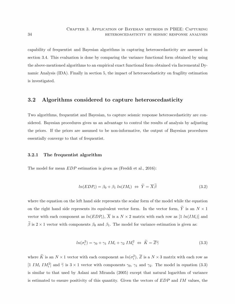
34Chapter 3. Application of Bayesian methods in PBEE: Capturing
heteroscedasticity in seismic response analyses
capability of frequentist and Bayesian algorithms in capturing heteroscedasticity are assessed in
section 3.4. This evaluation is done by comparing the variance functional form obtained by using
the above-mentioned algorithms to an empirical exact functional form obtained via Incremental Dy-
namic Analysis (IDA). Finally in section 5, the impact of heteroscedasticity on fragility estimation
is investigated.
3.2 Algorithms considered to capture heteroscedasticity
Two algorithms, frequentist and Bayesian, to capture seismic response heteroscedasticity are con-
sidered. Bayesian procedures gives us an advantage to control the results of analysis by adjusting
the priors. If the priors are assumed to be non-informative, the output of Bayesian procedures
essentially converge to that of frequentist.
3.2.1 The frequentist algorithm
The model for mean EDP estimation is given as (Freddi et al., 2016):
ln(EDPi) = β0 + β1 ln(IMi) ⇔ Y = Xβ (3.2)
where the equation on the left hand side represents the scalar form of the model while the equation
on the right hand side represents its equivalent vector form. In the vector form, Y is an N × 1
vector with each component as ln(EDPi), X is a N × 2 matrix with each row as [1 ln(IMi)] and
β is 2× 1 vector with components β0 and β1. The model for variance estimation is given as:
ln(σ2i ) = γ0 + γ1 IMi + γ2 IM2i ⇔ K = Zγ (3.3)
where K is an N × 1 vector with each component as ln(σ2i ), Z is a N × 3 matrix with each row as
[1 IMi IM2i ] and γ is 3 × 1 vector with components γ0, γ1 and γ2. The model in equation (3.3)
is similar to that used by Aslani and Miranda (2005) except that natural logarithm of variance
is estimated to ensure positivity of this quantity. Given the vectors of EDP and IM values, the
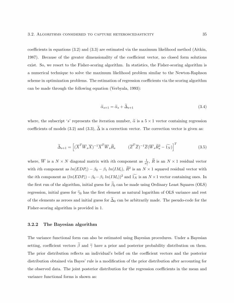
3.2. Algorithms considered to capture heteroscedasticity 35
coefficients in equations (3.2) and (3.3) are estimated via the maximum likelihood method (Aitkin,
1987). Because of the greater dimensionality of the coefficient vector, no closed form solutions
exist. So, we resort to the Fisher-scoring algorithm. In statistics, the Fisher-scoring algorithm is
a numerical technique to solve the maximum likelihood problem similar to the Newton-Raphson
scheme in optimization problems. The estimation of regression coefficients via the scoring algorithm
can be made through the following equation (Verbyala, 1993):
αs+1 = αs + ∆s+1 (3.4)
where, the subscript ‘s’ represents the iteration number, α is a 5 × 1 vector containing regression
coefficients of models (3.2) and (3.3), ∆ is a correction vector. The correction vector is given as:
∆s+1 =[(X
TW sX)−1X
TW sRs (Z
TZ)−1Z(W sR
2s − 1N )
]T(3.5)
where, W is a N × N diagonal matrix with ith component as 1σ2i, R is an N × 1 residual vector
with ith component as ln(EDPi)− β0 − β1 ln(IMi), R2 is an N × 1 squared residual vector with
the ith component as (ln(EDPi)−β0−β1 ln(IMi))2 and 1N is an N ×1 vector containing ones. In
the first run of the algorithm, initial guess for β0 can be made using Ordinary Least Squares (OLS)
regression, initial guess for γ0 has the first element as natural logarithm of OLS variance and rest
of the elements as zeroes and initial guess for ∆0 can be arbitrarily made. The pseudo-code for the
Fisher-scoring algorithm is provided in 1.
3.2.2 The Bayesian algorithm
The variance functional form can also be estimated using Bayesian procedures. Under a Bayesian
setting, coefficient vectors β and γ have a prior and posterior probability distribution on them.
The prior distribution reflects an individual’s belief on the coefficient vectors and the posterior
distribution obtained via Bayes’ rule is a modification of the prior distribution after accounting for
the observed data. The joint posterior distribution for the regression coefficients in the mean and
variance functional forms is shown as:
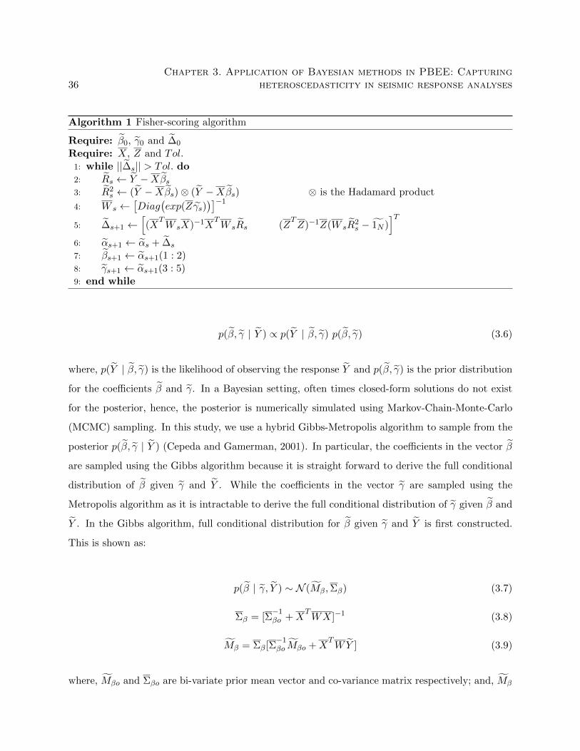
36Chapter 3. Application of Bayesian methods in PBEE: Capturing
heteroscedasticity in seismic response analyses
Algorithm 1 Fisher-scoring algorithm
Require: β0, γ0 and ∆0
Require: X, Z and Tol.1: while ||∆s|| > Tol. do2: Rs ← Y −Xβs3: R2
s ← (Y −Xβs)⊗ (Y −Xβs) ⊗ is the Hadamard product
4: W s ←[Diag
(exp(Zγs)
)]−15: ∆s+1 ←
[(X
TW sX)−1X
TW sRs (Z
TZ)−1Z(W sR
2s − 1N )
]T6: αs+1 ← αs + ∆s
7: βs+1 ← αs+1(1 : 2)8: γs+1 ← αs+1(3 : 5)9: end while
p(β, γ | Y ) ∝ p(Y | β, γ) p(β, γ) (3.6)
where, p(Y | β, γ) is the likelihood of observing the response Y and p(β, γ) is the prior distribution
for the coefficients β and γ. In a Bayesian setting, often times closed-form solutions do not exist
for the posterior, hence, the posterior is numerically simulated using Markov-Chain-Monte-Carlo
(MCMC) sampling. In this study, we use a hybrid Gibbs-Metropolis algorithm to sample from the
posterior p(β, γ | Y ) (Cepeda and Gamerman, 2001). In particular, the coefficients in the vector β
are sampled using the Gibbs algorithm because it is straight forward to derive the full conditional
distribution of β given γ and Y . While the coefficients in the vector γ are sampled using the
Metropolis algorithm as it is intractable to derive the full conditional distribution of γ given β and
Y . In the Gibbs algorithm, full conditional distribution for β given γ and Y is first constructed.
This is shown as:
p(β | γ, Y ) ∼ N (Mβ,Σβ) (3.7)
Σβ = [Σ−1βo +X
TWX]−1 (3.8)
Mβ = Σβ[Σ−1βo Mβo +X
TWY ] (3.9)
where, Mβo and Σβo are bi-variate prior mean vector and co-variance matrix respectively; and, Mβ

3.2. Algorithms considered to capture heteroscedasticity 37
and Σβ are bi-variate posterior mean vector and co-variance matrix respectively. In a Gibbs algo-
rithm, all the samples drawn from p(β | γ, Y ) are accepted. Given β, γ is sampled using Metropolis
algorithm. In a Metropolis algorithm, a proposal distribution for γ (γ∗) is first constructed. This
is shown as:
γ∗ ∼ N (Mγ ,Σγ) (3.10)
Σγ = [Σ−1γo + 0.5Z
TZ]−1 (3.11)
Mγ = Σγ [Σ−1γo Mγo + 0.5Z
TYt] (3.12)
where, Mγo and Σγo are tri-variate prior mean vector and co-variance matrix respectively; and, Mγ
and Σγ are tri-variate proposal mean vector and co-variance matrix respectively. A transformed
response variable (Yt) to achieve good acceptance rates in the Metropolis algorithm is expressed as
(Cepeda and Gamerman, 2001):
Yt = (Zγ − 1N ) + [WR2] (3.13)
After sampling a proposal vector γ∗ which contains the variance functional form coefficients,
the acceptance ratio (α) is calculated using (Hoff, 2009):
ln(α) = min
1, [sum(ln(dnorm(Y ,Xβs+1, σ∗)))
− sum(ln(dnorm(Y ,Xβs+1, σs)))]
+ ln(dnorm(γ∗, Mγo,Σγo))− ln(dnorm(γs, Mγo,Σγo)) (3.14)
where, dnorm is the normal density and σ is given by sqrt(exp(Zγ)). If α is greater than a
uniformly distributed random variable, we accept the proposal γ∗, otherwise, we reject it. The
pseudo-code for the Bayesian algorithm is provided in Algorithm 2.
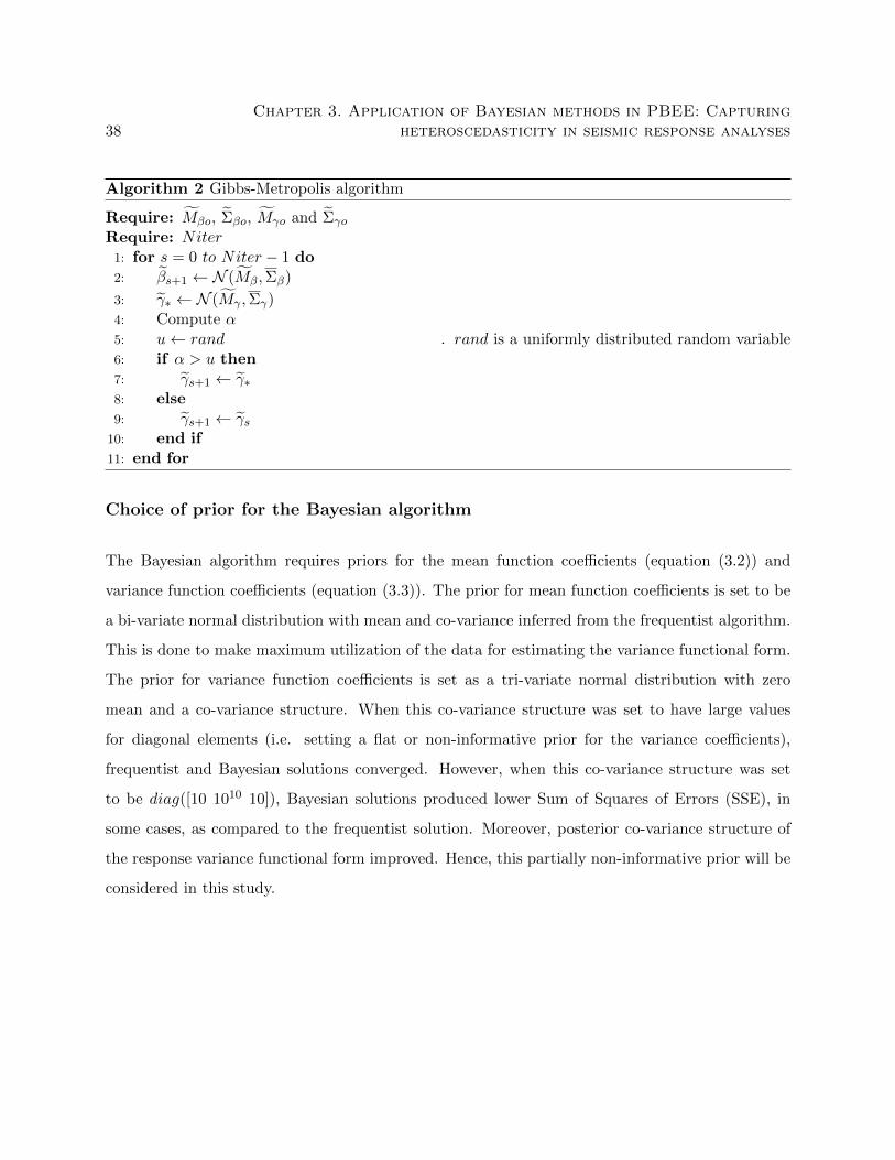
38Chapter 3. Application of Bayesian methods in PBEE: Capturing
heteroscedasticity in seismic response analyses
Algorithm 2 Gibbs-Metropolis algorithm
Require: Mβo, Σβo, Mγo and Σγo
Require: Niter1: for s = 0 to Niter − 1 do2: βs+1 ← N (Mβ,Σβ)
3: γ∗ ← N (Mγ ,Σγ)4: Compute α5: u← rand . rand is a uniformly distributed random variable6: if α > u then7: γs+1 ← γ∗8: else9: γs+1 ← γs
10: end if11: end for
Choice of prior for the Bayesian algorithm
The Bayesian algorithm requires priors for the mean function coefficients (equation (3.2)) and
variance function coefficients (equation (3.3)). The prior for mean function coefficients is set to be
a bi-variate normal distribution with mean and co-variance inferred from the frequentist algorithm.
This is done to make maximum utilization of the data for estimating the variance functional form.
The prior for variance function coefficients is set as a tri-variate normal distribution with zero
mean and a co-variance structure. When this co-variance structure was set to have large values
for diagonal elements (i.e. setting a flat or non-informative prior for the variance coefficients),
frequentist and Bayesian solutions converged. However, when this co-variance structure was set
to be diag([10 1010 10]), Bayesian solutions produced lower Sum of Squares of Errors (SSE), in
some cases, as compared to the frequentist solution. Moreover, posterior co-variance structure of
the response variance functional form improved. Hence, this partially non-informative prior will be
considered in this study.
3.3. Case study description 39
3.3 Case study description
Structure description
For investigating the performance of the frequentist and Bayesian algorithms in capturing het-
eroscedasticity, a four story steel moment frame building was considered. The building was de-
signed for seismic loads in metropolitan Los Angeles, CA. The fundamental time period of this
building is 1.33 seconds and the base shear coefficient of the structure is about 0.082. A model
for the two-dimensional frame on the EW perimeter was developed in OpenSees by Eads (2013).
Material nonlinearity was taken into account via a lumped plasticity approach. Second order (geo-
metric nonlinear) effects on this two-dimensional frame caused by non-tributary gravity loads were
modeled using a leaning column.
Ground motions
The heteroscedasticity-capturing algorithms were applied to the four-story steel moment frame
using the FEMA P695 far-field set. This record set has been used in many recent studies that
conducted seismic response analyses on structural models. The ranges of earthquake magnitude,
Joyner-Boore distance and PGA in the considered record set are 6.5-7.5, 7.1Km-26Km and 0.13g-
0.82g respectively. As it is intended to capture heteroscedasticity in structural response between
IM ranges 0.01g-2g for PGA and 0.01g-1.5g for Sa(T1 = 1.33s), an assemblage of ground motion
record sets was created using the FEMA record set and the same record set scaled twice and thrice.
Out of this assemblage, approximately eighty records were selected such that the IMs PGA and
Sa(T1 = 1.33s), independently, have an approximate uniform distribution within the considered
IM ranges. This was done to avoid a biased and hence erroneous estimation of variance functional
form by the algorithms due to concentration of large numbers of IM values within a narrow range.
Typical frequency distributions of the two IMs are shown in Figure 3.1.

40Chapter 3. Application of Bayesian methods in PBEE: Capturing
heteroscedasticity in seismic response analyses
0 0.5 1 1.5
Sa(T1 = 1.33s) (g)
0
1
2
3
4
5F
requency
0 0.5 1 1.5
PGA (g)
0
1
2
3
4
5
6
Fre
qu
en
cy
Figure 3.1: Typical frequency distributions of IMs: (a) Sa(T1 = 1.33s) and (b) PGA used for theanalysis.
3.4 Results
The frequentist and Bayesian algorithms described in section 3.2 were applied to the structure
described in section 3.3. A MATLAB code has been developed to implement the above-mentioned
algorithms. The EDPs considered in this analysis are Inter-story Drift Ratio (IDR) and Peak
Floor Acceleration (PFA) at all four stories, Roof Drift (RD) of the structure and middle node
Joint Rotation at second story (JR). As mentioned earlier, the IMs Sa(T1 = 1.33s) and PGA are
considered independently in order to study their effectiveness in predicting the variance functional
form for different EDPs.
The variance functional forms predicted by the two algorithms are evaluated by computing
the Sum of Squares of Errors (SSE) with reference to IDA data. IDA was conducted using the
forty-four ground motion records (both the horizontal components considered) of FEMA record
set. For each of the two IMs, ground motion records were scaled with an interval of 0.05g until
1.5g for Sa(T1 = 1.33s) and until 2g for PGA, independently. During the scaling process some
earthquake records caused the structure to collapse. These collapse-causing earthquake records
were discarded from further analysis, i.e., they were not subjected to further scaling. Given an
IM level and the no-collapse EDP values from the analysis, the standard deviation in EDP values
was computed. Finally, given an EDP and IM, a variance functional form similar to that shown
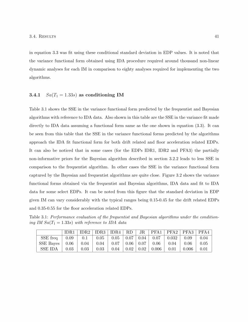
3.4. Results 41
in equation 3.3 was fit using these conditional standard deviation in EDP values. It is noted that
the variance functional form obtained using IDA procedure required around thousand non-linear
dynamic analyses for each IM in comparison to eighty analyses required for implementing the two
algorithms.
3.4.1 Sa(T1 = 1.33s) as conditioning IM
Table 3.1 shows the SSE in the variance functional form predicted by the frequentist and Bayesian
algorithms with reference to IDA data. Also shown in this table are the SSE in the variance fit made
directly to IDA data assuming a functional form same as the one shown in equation (3.3). It can
be seen from this table that the SSE in the variance functional forms predicted by the algorithms
approach the IDA fit functional form for both drift related and floor acceleration related EDPs.
It can also be noticed that in some cases (for the EDPs IDR1, IDR2 and PFA3) the partially
non-informative priors for the Bayesian algorithm described in section 3.2.2 leads to less SSE in
comparison to the frequentist algorithm. In other cases the SSE in the variance functional form
captured by the Bayesian and frequentist algorithms are quite close. Figure 3.2 shows the variance
functional forms obtained via the frequentist and Bayesian algorithms, IDA data and fit to IDA
data for some select EDPs. It can be noted from this figure that the standard deviation in EDP
given IM can vary considerably with the typical ranges being 0.15-0.45 for the drift related EDPs
and 0.35-0.55 for the floor acceleration related EDPs.
Table 3.1: Performance evaluation of the frequentist and Bayesian algorithms under the condition-ing IM Sa(T1 = 1.33s) with reference to IDA data
IDR1 IDR2 IDR3 IDR4 RD JR PFA1 PFA2 PFA3 PFA4
SSE freq 0.09 0.1 0.05 0.05 0.07 0.04 0.07 0.032 0.09 0.04SSE Bayes 0.06 0.04 0.04 0.07 0.06 0.07 0.06 0.04 0.06 0.05SSE IDA 0.03 0.03 0.03 0.04 0.02 0.02 0.006 0.01 0.006 0.01
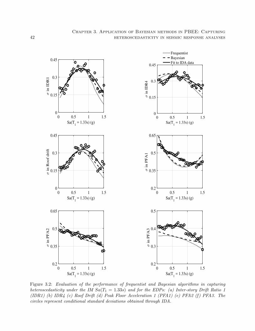
42Chapter 3. Application of Bayesian methods in PBEE: Capturing
heteroscedasticity in seismic response analyses
0 0.5 1 1.5
Sa(T1 = 1.33s) (g)
0
0.15
0.3
0.45
σ i
n I
DR
1
0 0.5 1 1.5
Sa(T1 = 1.33s) (g)
0
0.15
0.3
0.45
σ i
n I
DR
4
Frequentist
Bayesian
Fit to IDA data
0 0.5 1 1.5
Sa(T1 = 1.33s) (g)
0
0.15
0.3
0.45
σ i
n R
oo
f d
rift
0 0.5 1 1.5
Sa(T1 = 1.33s) (g)
0.2
0.35
0.5
0.65
σ i
n P
FA
1
0 0.5 1 1.5
Sa(T1 = 1.33s) (g)
0.2
0.35
0.5
0.65
σ i
n P
FA
2
0 0.5 1 1.5
Sa(T1 = 1.33s) (g)
0.2
0.3
0.4
0.5
σ i
n P
FA
3
Figure 3.2: Evaluation of the performance of frequentist and Bayesian algorithms in capturingheteroscedasticity under the IM Sa(T1 = 1.33s) and for the EDPs: (a) Inter-story Drift Ratio 1(IDR1) (b) IDR4 (c) Roof Drift (d) Peak Floor Acceleration 1 (PFA1) (e) PFA2 (f) PFA3. Thecircles represent conditional standard deviations obtained through IDA.
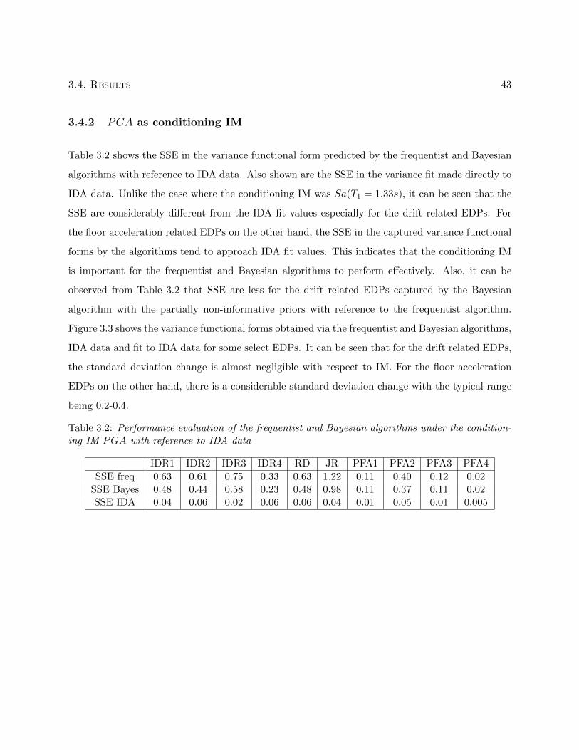
3.4. Results 43
3.4.2 PGA as conditioning IM
Table 3.2 shows the SSE in the variance functional form predicted by the frequentist and Bayesian
algorithms with reference to IDA data. Also shown are the SSE in the variance fit made directly to
IDA data. Unlike the case where the conditioning IM was Sa(T1 = 1.33s), it can be seen that the
SSE are considerably different from the IDA fit values especially for the drift related EDPs. For
the floor acceleration related EDPs on the other hand, the SSE in the captured variance functional
forms by the algorithms tend to approach IDA fit values. This indicates that the conditioning IM
is important for the frequentist and Bayesian algorithms to perform effectively. Also, it can be
observed from Table 3.2 that SSE are less for the drift related EDPs captured by the Bayesian
algorithm with the partially non-informative priors with reference to the frequentist algorithm.
Figure 3.3 shows the variance functional forms obtained via the frequentist and Bayesian algorithms,
IDA data and fit to IDA data for some select EDPs. It can be seen that for the drift related EDPs,
the standard deviation change is almost negligible with respect to IM. For the floor acceleration
EDPs on the other hand, there is a considerable standard deviation change with the typical range
being 0.2-0.4.
Table 3.2: Performance evaluation of the frequentist and Bayesian algorithms under the condition-ing IM PGA with reference to IDA data
IDR1 IDR2 IDR3 IDR4 RD JR PFA1 PFA2 PFA3 PFA4
SSE freq 0.63 0.61 0.75 0.33 0.63 1.22 0.11 0.40 0.12 0.02SSE Bayes 0.48 0.44 0.58 0.23 0.48 0.98 0.11 0.37 0.11 0.02SSE IDA 0.04 0.06 0.02 0.06 0.06 0.04 0.01 0.05 0.01 0.005
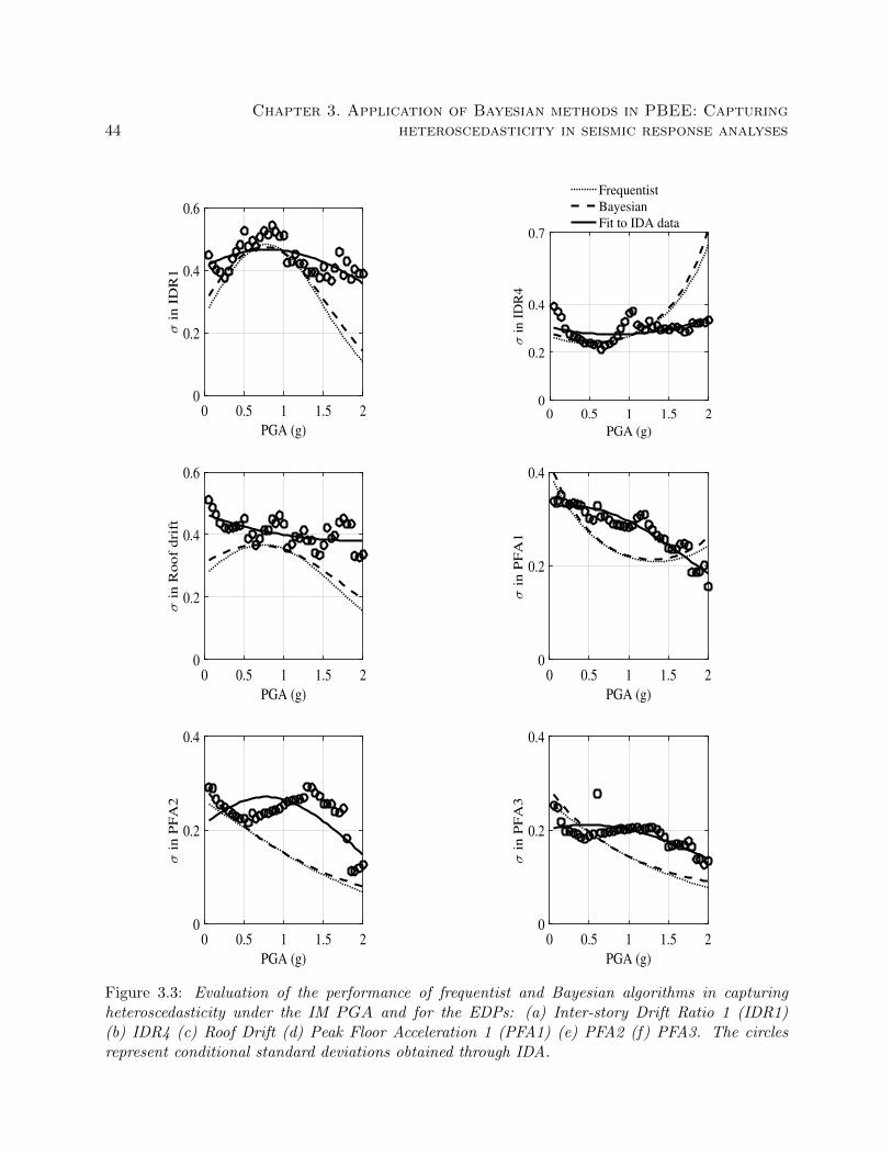
44Chapter 3. Application of Bayesian methods in PBEE: Capturing
heteroscedasticity in seismic response analyses
0 0.5 1 1.5 2
PGA (g)
0
0.2
0.4
0.6
σ i
n I
DR
1
0 0.5 1 1.5 2
PGA (g)
0
0.2
0.4
0.7
σ i
n I
DR
4
Frequentist
Bayesian
Fit to IDA data
0 0.5 1 1.5 2
PGA (g)
0
0.2
0.4
0.6
σ i
n R
oof
dri
ft
0 0.5 1 1.5 2
PGA (g)
0
0.2
0.4
σ i
n P
FA
1
0 0.5 1 1.5 2
PGA (g)
0
0.2
0.4
σ i
n P
FA
2
0 0.5 1 1.5 2
PGA (g)
0
0.2
0.4
σ i
n P
FA
3
Figure 3.3: Evaluation of the performance of frequentist and Bayesian algorithms in capturingheteroscedasticity under the IM PGA and for the EDPs: (a) Inter-story Drift Ratio 1 (IDR1)(b) IDR4 (c) Roof Drift (d) Peak Floor Acceleration 1 (PFA1) (e) PFA2 (f) PFA3. The circlesrepresent conditional standard deviations obtained through IDA.
3.5. Impact on fragility estimation 45
3.5 Impact on fragility estimation
To investigate the impact of heteroscedasticity on fragility estimation the EDP and IM are con-
sidered to be Roof Drift (RD) and Sa(T1 = 1.33s) respectively. RD is often an EDP of interest
during probabilistic seismic loss assessment and as noted previously, the heteroscedasticity captur-
ing algorithms perform well when the conditioning IM is Sa(T1 = 1.33s). Figure 3.4 shows the
fragility curves for the RD values 0.02, 0.03, 0.04 and 0.045. Three methods, IDA, GLM algorithm
and homoscedasticity, were used to obtain the fragility curves. In the IDA method the variance
functional form directly fit to IDA data was used, in the GLM method the Bayesian algorithm
was used to estimate the variance functional form utilizing limited data and constant variance
was assumed across all IM levels in the homoscedasticity method. Upon obtaining the variance
functional form, equation (3.1) was used to obtain the fragility curves. It can be observed from
Figure 3.4 that at lower levels of RD considering heteroscedasticity does not make any difference in
fragility estimation. However, at high levels of RD (>0.03) considering heteroscedasticity changes
the fragility estimates noticeably from assuming homoscedasticity. Also, the algorithms used in
this here are able to reproduce fragility curves which match closely with IDA method.
3.6 Conclusions
This study has applied two algorithms, frequentist and Bayesian, to capture seismic response het-
eroscedasticity (standard deviation change) in a four story steel moment frame building. The
following conclusions can be drawn:
• In line with previous research, the standard deviation in EDP is found to vary considerably
with IM level. Typical range of standard deviation was found to be 0.15-0.45 for the drift
related EDPs and 0.35-0.55 for the floor acceleration related EDPs under the IM Sa(T1 =
1.33s). For the IM PGA on the other hand, the standard deviation did not vary considerably
with IM level for the drift related EDPs while the standard deviation ranged between 0.2-0.4
for the floor acceleration related EDPs.
• The frequentist and Bayesian algorithms performed well in capturing variance change as a
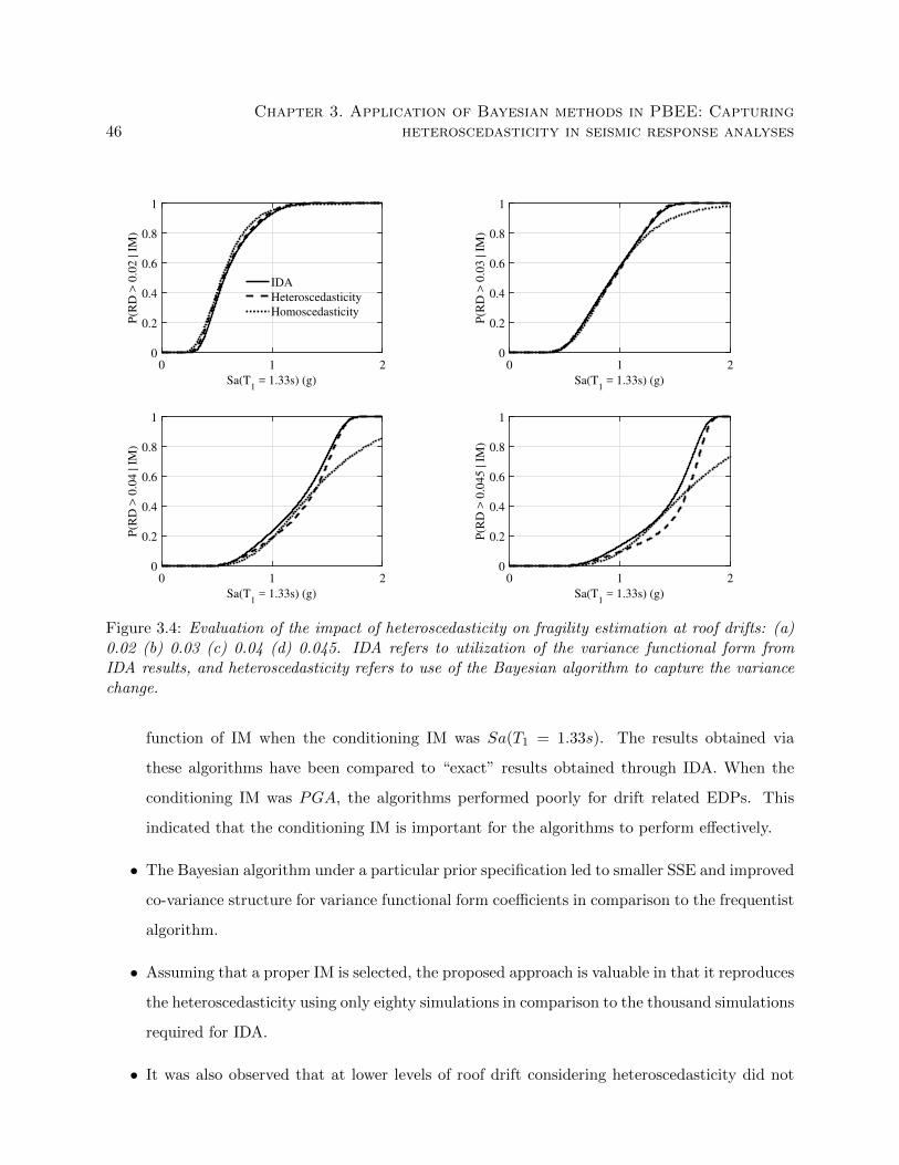
46Chapter 3. Application of Bayesian methods in PBEE: Capturing
heteroscedasticity in seismic response analyses
0 1 2
Sa(T1 = 1.33s) (g)
0
0.2
0.4
0.6
0.8
1
P(R
D >
0.0
2 | I
M)
IDA
Heteroscedasticity
Homoscedasticity
0 1 2
Sa(T1 = 1.33s) (g)
0
0.2
0.4
0.6
0.8
1
P(R
D >
0.0
3 | I
M)
0 1 2
Sa(T1 = 1.33s) (g)
0
0.2
0.4
0.6
0.8
1
P(R
D >
0.0
4 | I
M)
0 1 2
Sa(T1 = 1.33s) (g)
0
0.2
0.4
0.6
0.8
1
P(R
D >
0.0
45
| I
M)
Figure 3.4: Evaluation of the impact of heteroscedasticity on fragility estimation at roof drifts: (a)0.02 (b) 0.03 (c) 0.04 (d) 0.045. IDA refers to utilization of the variance functional form fromIDA results, and heteroscedasticity refers to use of the Bayesian algorithm to capture the variancechange.
function of IM when the conditioning IM was Sa(T1 = 1.33s). The results obtained via
these algorithms have been compared to “exact” results obtained through IDA. When the
conditioning IM was PGA, the algorithms performed poorly for drift related EDPs. This
indicated that the conditioning IM is important for the algorithms to perform effectively.
• The Bayesian algorithm under a particular prior specification led to smaller SSE and improved
co-variance structure for variance functional form coefficients in comparison to the frequentist
algorithm.
• Assuming that a proper IM is selected, the proposed approach is valuable in that it reproduces
the heteroscedasticity using only eighty simulations in comparison to the thousand simulations
required for IDA.
• It was also observed that at lower levels of roof drift considering heteroscedasticity did not

3.6. Conclusions 47
affect fragility estimation. However, at high levels of roof drift (>0.03) considering het-
eroscedasticity resulted in a closer match to IDA results than the homoscedastic assumption.
Chapter 4
A unified metric for the quality
assessment of scalar intensity
measures that characterize an
earthquake
This chapter expands upon a study excerpted from:
Somayajulu L.N. Dhulipala, Adrian Rodriguez-Marek, Shyam Ranganathan, and Madeleine M.
Flint. “A siteconsistent method to quantify sufficiency of alternative IMs in relation to PSDA.”
Earthquake Engineering & Structural Dynamics 47(2) 2018: 377-396.
4.1 Introduction
Performance-Based Earthquake Engineering (PBEE, Moehle and Deierlein 2004) quantifies the un-
certainty in a building’s loss due to an earthquake in terms of annual frequency of exceedance (AFE).
The PEER framework for PBEE propagates uncertainties in earthquake events to uncertainties in
ground motion at a site (hazard analysis), to uncertainties in structural response (demand analysis),
to uncertainties in structural damage (damage analysis) and finally to uncertainties in loss variables
(loss analysis). The demand analysis phase of the PEER framework is referred to as Probabilistic
Seismic Demand Analysis (PSDA). In traditional PSDA, the annual frequency of exceedance of a
demand variable is computed by probabilistically linking structural response to a scalar earthquake
Intensity Measure (IM) (Ebrahimian et al., 2015; Jalayer et al., 2012). This utilization of a scalar
48
4.1. Introduction 49
IM facilitates the implementation of PBEE through the PEER framework formula (Moehle and
Deierlein, 2004). However, it is implicitly assumed that structural response is only dependent on
the scalar IM, and is fully independent of other earthquake and ground motion properties (referred
to herein as seismological parameters): this assumption is known as the conditional independence.
Luco and Cornell (2007) define conditional independence as a sufficiency criterion of scalar IMs to
avoid a biased evaluation of the seismic demand hazard (Giovenale et al., 2004). Unless otherwise
mentioned, in this study we treat sufficiency as per this definition.
Conditional independence of structural response from seismological parameters such as magni-
tude (M), distance (R) and epsilon (ε, the normalized difference between the natural logarithms of
observed and predicted values of IM) is desirable. This independence legitimizes the conditioning
of response on a scalar IM in PSDA (Jalayer et al., 2015; Luco and Cornell, 2007). Conditional
independence also legitimizes the linear scaling of ground motion records in an incremental dynamic
analysis (Vamvatsikos and Cornell, 2002) to find the collapse capacity of structures (Eads et al.,
2013).
Recognizing the statistical and practical significance of conditional independence, much effort
has been put into finding optimal IMs that render structural response independent of seismological
parameters. Luco and Cornell (2007) propose the use of null hypothesis tests to assess whether
different seismological parameters are statistically significant in relation to structural response. In
such a test, a p-value is calculated to assess the dependence of residuals in predicted response, given
an IM , on any seismological parameter (Luco and Cornell, 2007). A p-value is the probability of
obtaining a result equal to or more extreme than what was actually observed. If the p-value exceeds
a pre-defined significance level, then the structural response can be declared to be statistically
independent from the seismological parameter under consideration. Padgett et al. (2008) use a
similar approach to assess the sufficiency of alternative scalar IMs in relation to responses of a
portfolio of bridges, using both recorded and synthetic ground motions. More recently, Hariri-
Ardebili and Saouma (2016) use the same approach to assess the sufficiency of a large suite of
alternative IMs in relation to the response of a gravity dam.
Efficiency of a scalar IM is a complimentary criterion to sufficiency. Relative efficiencies of
IMs are gauged by comparing the standard deviations these IMs induce in predicting structural
50Chapter 4. A unified metric for the quality assessment of scalar intensity
measures that characterize an earthquake
response. The previously mentioned studies of sufficiency (Hariri-Ardebili and Saouma, 2016; Luco
and Cornell, 2007; Padgett et al., 2008), as well as many others (Shakib and Jahangiri, 2016), find
that it is possible for multiple IMs to pass the null hypothesis test irrespective of their efficiencies
in predicting structural response. Also, the relation between efficiency and sufficiency of IMs is
unclear in the PEER PBEE framework.
A common problem faced in prior work (Bradley et al., 2009; Freddi et al., 2016; Hariri-
Ardebili and Saouma, 2016; Luco and Cornell, 2007; Shakib and Jahangiri, 2016) is the difficulty
of determining which IM is most sufficient when multiple IMs pass/fail the null hypothesis test
(i.e., have acceptable p-values greater/less than the significance level). Historically, the choice of
significance level has been subjective. Bradley et al. (2009) use a significance value of 0.05 while
Padgett et al. (2008) use a value of 0.1. More concerning is that p-values are, from a statistical
point of view, not measures of support (Schervish, 1996). That is, p-values can tell us whether
different seismological parameters are statistically significant or not given an IM , but they cannot
gauge the relative degree to which different IMs are sufficient.
Apart from the difficulties associated with subjectivity and lack of a basis for relative assess-
ment of IM sufficiency, the p-value approach does not take into consideration the site hazard.
Some studies (Kohrangi et al., 2016a; Vamvatsikos, 2015) have stated that if an IM is sufficient,
this sufficiency would allow selection of ground motion records to be independent of the site hazard
under consideration. However, the conventional approach of evaluating sufficiency considers only
the distribution of seismological parameters within the ground motion record set used for analysis.
In almost all of the prior studies assessing sufficiency of alternative IMs, ground motion record sets
were not selected consistently with the site hazard (see for example Bradley et al. 2009; Ebrahimian
et al. 2015). Traditionally, sufficiency has been treated as a property only of the IM . However,
site hazard and the quality of ground motion record set selected can also play an important role in
determining an IM ’s performance in rendering sufficiency.
We propose an approach to evaluate the degree of sufficiency of scalar IMs. This approach
evaluates the degree of total dependence of structural response on various seismological param-
eters, at different response levels, using a pre-defined regression model. As the new approach
computes the total information gain to assess the degree of sufficiency, it supports comparison of

4.1. Introduction 51
the performance of different scalar IMs given a specific response quantity and across various re-
sponse quantities. Computing the total information gain taking into account site hazard requires
continuous deaggregation across the IM space. Continuous deaggregation is impractical for rea-
sons of computational expense, so we also propose an approximate deaggregation technique. The
approximate deaggregation technique allows for continuous estimation of marginal deaggregation
probabilities given deaggregation at coarse IM intervals. Using the new metric for sufficiency,
we investigate the influence of ground motion selection on degree of sufficiency of alternate IMs,
thereby assessing the quality of different ground motion record sets in rendering IM sufficiency.
Finally, we study the relation between the proposed total information gain and standard deviation
in structural response given an IM (efficiency). We observe that the natural logarithm of the
proposed metrics for sufficiency and efficiency are consistent with a bi-variate normal distribution.
This conclusion is further utilized to develop a unified metric that gauges both the sufficiency and
the efficiency of scalar IMs.
Jalayer et al. (2012) propose a Relative Sufficiency Measure (RSM) which assesses the ground
motion representation capability of one IM in relation to another. In Appendix A, we perform some
mathematical manipulations on the approximate RSM and find that ground motion representation
capability of IMs can be conveniently gaged by comparing the standard deviations they render
in predicting EDP . Hence, RSM is a measure of the relative efficiency of two IMs. Moreover,
the approximate RSM neither takes into consideration the seismological parameters nor does it
evaluate the conditional independence of EDP from seismological parameters given IM . For this
reason, we focus on the Luco and Cornell (2007) definition of sufficiency.
The proposed approach for quantifying sufficiency is applied to a case study structure consid-
ering various response quantities and IMs as described in section 4.2. Section 4.3 mathematically
describes the alternative approach, investigates the degree of sufficiency of various scalar IMs across
different structural response quantities, and proposes and evaluates the approximate de-aggregation
approach. Section 4.4 evaluates the influence of ground motion record set on sufficiency. Section
4.5 investigates the relation between the proposed total information gain metric for sufficiency and
the standard deviation metric for efficiency. In appendix A, a logical consequence of the RSM is
presented.
52Chapter 4. A unified metric for the quality assessment of scalar intensity
measures that characterize an earthquake
4.2 Case study description
This section describes a case study which will be used to demonstrate the proposed metric for
sufficiency and further evaluate its implications.
4.2.1 Structure description
The structure analyzed is a four-story steel perimeter moment frame building located in Los Ange-
les, California. The building has been designed for a seismic base shear co-efficient of V/W = 0.082.
A two-dimensional model of the east-west frame of the building was created in OpenSees by Eads
et al. (2013). Material non-linearity is accounted for using a concentrated plasticity model having
both strength and stiffness degradation (Ibarra et al., 2005). A leaning column is used to simulate
P -∆ effects, i.e., the effects of non-tributary gravity loads on the two-dimensional frame that is
explicitly modeled. For more details about the structure geometry and modeling, the reader is
referred to Eads (2013).
4.2.2 Intensity measures, structural response quantities and seismological pa-
rameters
A total of eight simple IMs were considered in this study. Three of the IMs are spectral accelera-
tions at first three fundamental mode periods, Sa(T1 = 1.33s), Sa(T2 = 0.43s) and Sa(T3 = 0.22s).
To study the effects of extended mode period on degree of conditional independence, Sa(1.5s) was
also considered. Spectral accelerations at structure-independent periods of 1s and 2s (Sa(1s) and
Sa(2s)) were also considered. Finally, peak ground acceleration and velocity (PGA and PGV )
were considered.
In order evaluate the performance of the above-mentioned IMs across multiple EDP s, the
response quantities adopted in this study are peak: roof drift (RD); inter-story drift ratios at first
and fourth stories (IDR1 and IDR4); middle-node joint rotation at the second story (JR); and
floor accelerations at the first and fourth stories (PFA1 and PFA4). In this study conditional
independence of EDP given IM is assessed from three seismological parameters: Magnitude (M),
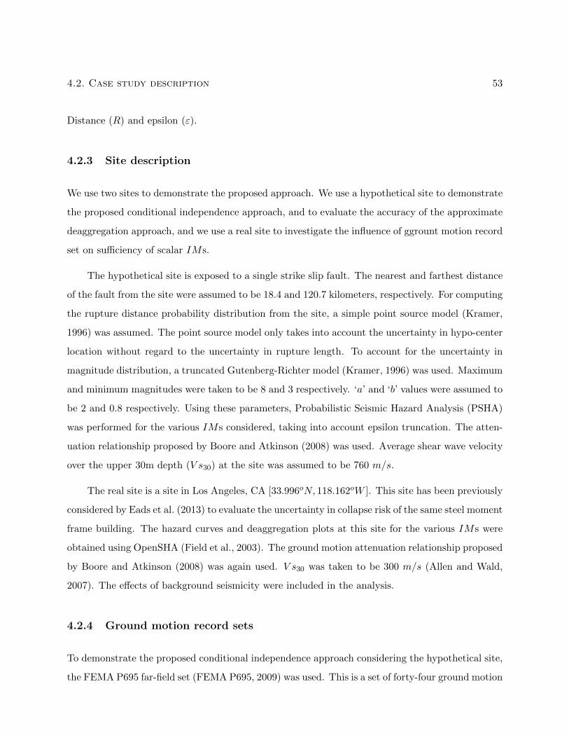
4.2. Case study description 53
Distance (R) and epsilon (ε).
4.2.3 Site description
We use two sites to demonstrate the proposed approach. We use a hypothetical site to demonstrate
the proposed conditional independence approach, and to evaluate the accuracy of the approximate
deaggregation approach, and we use a real site to investigate the influence of ggrount motion record
set on sufficiency of scalar IMs.
The hypothetical site is exposed to a single strike slip fault. The nearest and farthest distance
of the fault from the site were assumed to be 18.4 and 120.7 kilometers, respectively. For computing
the rupture distance probability distribution from the site, a simple point source model (Kramer,
1996) was assumed. The point source model only takes into account the uncertainty in hypo-center
location without regard to the uncertainty in rupture length. To account for the uncertainty in
magnitude distribution, a truncated Gutenberg-Richter model (Kramer, 1996) was used. Maximum
and minimum magnitudes were taken to be 8 and 3 respectively. ‘a’ and ‘b’ values were assumed to
be 2 and 0.8 respectively. Using these parameters, Probabilistic Seismic Hazard Analysis (PSHA)
was performed for the various IMs considered, taking into account epsilon truncation. The atten-
uation relationship proposed by Boore and Atkinson (2008) was used. Average shear wave velocity
over the upper 30m depth (V s30) at the site was assumed to be 760 m/s.
The real site is a site in Los Angeles, CA [33.996oN, 118.162oW ]. This site has been previously
considered by Eads et al. (2013) to evaluate the uncertainty in collapse risk of the same steel moment
frame building. The hazard curves and deaggregation plots at this site for the various IMs were
obtained using OpenSHA (Field et al., 2003). The ground motion attenuation relationship proposed
by Boore and Atkinson (2008) was again used. V s30 was taken to be 300 m/s (Allen and Wald,
2007). The effects of background seismicity were included in the analysis.
4.2.4 Ground motion record sets
To demonstrate the proposed conditional independence approach considering the hypothetical site,
the FEMA P695 far-field set (FEMA P695, 2009) was used. This is a set of forty-four ground motion
54Chapter 4. A unified metric for the quality assessment of scalar intensity
measures that characterize an earthquake
records (both the horizontal components), with magnitudes ranging from 6.5-7.5 and distances
ranging from 7.1 Km-26 Km.
To further apply the proposed conditional independence procedure to the real site, and thereby
to investigate the influence of ground motion selection on conditional independence, three additional
ground motion sets were considered: the Medina-Krawinkler LMSR-N set, and two sets related to
the Conditional Spectrum (CS) approach of Lin et al. (2013b). The Medina-Krawinkler LMSR-N
set (Medina, 2003) contains forty ground motions, with magnitudes ranging from 6.5-7 and distances
ranging from 13 Km-40 Km. The final two record sets were selected using the CS approach, which
takes into account both the conditional mean and variability of spectral accelerations at various
oscillator periods. Computing the CS requires seed values of M , R, ε and conditioning period. The
seed values for M , R and ε (6.77, 17.18 Kilometers and 1.53) were taken as the mean values obtained
by conducting a deaggregation of the hazard at a 2475-years return period. The conditioning
period was taken as the structure’s fundamental elastic period (1.33s). Ground motions were not
scaled while matching the conditional mean spectrum or target variability in order to support the
investigation of the conditional independence of structural response given IM from non-scalable
seismological parameters. Fifty seven ground motions from the PEER strong motion database were
selected using the selection algorithm of Jayaram et al. (2011). The conditional mean spectrum
and the conditional standard deviation at different periods are shown in Figure 4.1, along with the
response spectra of the selected ground motions. Out of the fifty seven selected ground motions,
twenty-six were identified as pulse-like (Shahi and Baker, 2012). The ground motions matching the
CS were therefore divided into two sets of non-pulse-like and pulse-like ground motions. Finally,
it is acknowledged that conditioning the CS at a particular oscillator period and investigating the
sufficiency of spectral accelerations at other time periods may be considered inconsistent, however,
it was determined to be appropriate for the purpose of investigating the influence of different ground
motion sets on IM sufficiency.
4.3. Site hazard consistent conditional independence assessment of alternativeIntensity Measures 55
T (s)
10-1
100
101
Sa
(g)
10-2
10-1
100
Response spectra of selected ground motions
2.5 and 97.5 percentile response spectra
Median response spectrum
(a)
T (s)
10-1
100
101
Sta
ndar
d d
evia
tion o
f ln
Sa
0
0.2
0.4
0.6
0.8
1
Target standard deviation of lnSa
Standard deviation of selected lnSa
(b)
Figure 4.1: (a) Conditional mean spectrum and fifty seven matched ground motions; (b) Variabilityin the target and sample conditional response spectrum
4.3 Site hazard consistent conditional independence assessment of
alternative Intensity Measures
4.3.1 Mathematical description of the proposed approach
Preliminaries related to IM , EDP , and seismological parameters
Let φ = (φ1, φ2, ...) be a vector of ground motion or seismological parameters (e.g., earthquake
magnitude M , distance R and epsilon ε) against which conditional independence of response is
to be assessed. Let IMi be the ith ground motion intensity measure in a suite of alternative
intensity measures. Let EDP be the structural response quantity under consideration. Assume
that the median EDP and IMi are related assuming a pre-defined empirical relation (such as
ˆEDP = F (IMi)). The probability of exceedence of a value of EDP given IMi is:
Pr(EDP > y|IMi) = 1− Φ( lny − F (IMi)
βEDP |IMi
)(4.1)
where Φ denotes the cumulative normal distribution function and βEDP |IMiis the standard de-
56Chapter 4. A unified metric for the quality assessment of scalar intensity
measures that characterize an earthquake
viation in predicting EDP given IMi. Further, assume that the EDP , IMi and φj , the jth
seismological parameter under consideration, are also related by an empirical relation (such as
EDP = F (IMi, φj)). The probability of exceedence of a value of EDP given IMi and φj
(P r(EDP > y|IMi, φj)) can be calculated in a similar manner as in equation (4.1). Considering
the jth seismological parameter, the probability of exceedence of a value of EDP given IMi can
be obtained using the total probability theorem (Benjamin and Cornell, 2014). Such an operation
is given by:
P r(EDP > y|IMi) =
∫φj
Pr(EDP > y|IMi, φj) f(φj |IMi) dφj (4.2)
where f(φj |IMi) denotes the density distribution of φj given an IM level. Note that P r(EDP >
y|IM) denotes the conditional probability of exceedance of EDP given IMi having taken into
consideration the j seismological parameter. For example, if φj is the magnitude of earthquake,
the distribution f(φj |IMi) can be obtained by deaggregation. Whenever a seismological parameter
is independent of the IM level under consideration, its conditioning on IMi can be omitted in
equation (4.2). It is noted that the exceedence probability is calculated by assuming an appropriate
probability model for the residuals in the empirical relations. More details of the empirical and
probability models will be provided in section 4.3.2.
IM sufficiency would imply independence of the EDP |IMi relationship from the seismological
parameters (Luco and Cornell, 2007). A divergence between the demand fragilities obtained without
and with considering φj (Pr(EDP > y|IMi) and P r(EDP > y|IMi)) would indicate the influence
of this seismological parameter. Divergence measures between Cumulative Distribution Functions
(CDF), however, have the same dimension as the IM under consideration and hence cannot be used
for comparison across different classes of IMs. In addition, upon accounting for the seismological
parameter (φj), if two IMs had the same effect on the EDP |IMi relationship, the computed
divergences between CDFs (i.e., between Pr(EDP > y|IMi) and P r(EDP > y|IMi) for each of
the two IMs) may be biased in favor of the more efficient IM among the two. This is because, for
the same influence of a seismological parameter, an efficient IM would have lesser area enclosed
between the CDFs than an inefficient one. To circumvent these issues, we use Bayes rule (Hoff, 2009)
4.3. Site hazard consistent conditional independence assessment of alternativeIntensity Measures 57
to multiply the demand fragility with the slope of seismic hazard curve to give an IMi|EDP > y
density distribution as shown below:
f(IMi|EDP > y) =Pr(EDP > y|IMi) |dλ(IMi)
dIMi|∫
IMi
Pr(EDP > y|IMi) |dλ(IMi)dIMi
|dIMi
(4.3)
where λ(IMi) denotes the seismic hazard curve for the ith IM in the suite. When considering the
jth seismological parameter, a density distribution can be obtained in a similar fashion and will
be denoted by fj(IMi|EDP > y). Divergences between density functions (f(IMi|EDP > y) and
fj(IMi|EDP > y)), unlike CDFs, do not depend on the dimension of the IM . Also, measuring
differences between density functions allows for a neutral treatment to gauge the influence of a
seismological parameter on EDP |IMi relation across all combinations of EDP s and IMs. Finally,
it is noted that obtaining the above-mentioned density distributions requires information about
deaggregation in equation (4.2) and seismic hazard in equation (4.3) which are site specific.
A measure for IM sufficiency
Here, we employ principles of information theory (Cover and Joy, 2012) to assess the degree of
conditional independence of scalar IMs.
We have two IMi density distributions f(IMi|EDP > y) and fj(IMi|EDP > y). The latter
density distribution considers the influence of jth seismological parameter on EDP while the former
does not. So, there is a gain of information due to inclusion of the seismological parameter while
considering the distribution fj(IMi|EDP > y) in comparison to the distribution f(IMi|EDP > y).
Mathematically, information gain is measured using Kullback-Liebler divergence1 (Cover and Joy,
2012; Jalayer et al., 2012):
IGij(y) =
∫IMi
fj(IMi|EDP > y) log2fj(IMi|EDP > y)
f(IMi|EDP > y)dIMi (4.4)
1The Kullback-Liebler divergence is sometimes referred to as relative entropy or weighted average informationgain or simply information gain.
58Chapter 4. A unified metric for the quality assessment of scalar intensity
measures that characterize an earthquake
where IGij(y) is information gain at response level y considering ith IM and jth seismological pa-
rameter. The Kullback-Leibler divergence (KL divergence) computes how much gain of information
there is in terms of bits due to the use of the model with seismological parameter fj(IMi|EDP > y)
in comparison to the model f(IMi|EDP > y). In other words, it compares how different these two
densities are. But the KL divergence is not to be interpreted as a conventional distance metric,
because it neither is symmetric nor does it satisfy the triangle inequality (Cover and Joy, 2012). If
the KL divergence is zero then the densities f(IMi|EDP > y) and fj(IMi|EDP > y) are same and
considering jth seismological parameter does not affect the EDP |IMi relationship. This is because
the demand fragilities obtained without and with the seismological parameter (Pr(EDP > y|IMi)
and P r(EDP > y|IMi)) are convolved with the same seismic hazard curve given an IM as shown
in equation (4.3); and a zero KL divergence would also imply these demand fragilities are the same.
Alternatively, one might prefer measuring the divergences between the EDP |IM density dis-
tributions with and without considering the seismological parameter. Such an operation gives
information gain which is dependent on the IM level under consideration and hence cannot be
compared across different IMs.
The Total Information Gain (TIGi(y)) under the ith IM due to all the seismological param-
eters considered (φ) is simply the sum of information gains attributable to the individual seismo-
logical parameters (φj). This final equation for the conditional independence metric of a given IM
and response level is:
TIGi(y) =
Nφ∑j=1
IGij(y) (4.5)
where it is assumed that all the seismological parameters in the vector (φ) are strictly independent
in population, i.e., they have no common information content. Or in other words, the mutual
information (Cover and Joy, 2012) between the seismological parameters is assumed to be zero.
An implication of this assumption is that the effects of all the seismological parameters on the
structural response may be considered individually.
Finally, sufficiency must be compared across the alternative IMs. Given a vector of alternative
4.3. Site hazard consistent conditional independence assessment of alternativeIntensity Measures 59
scalar IMs, an IM is most sufficient if it has the least total information gain. This is shown as:
IMsuff (y) = argmini TIGi(y) (4.6)
4.3.2 Empirical models relating EDP − IMi and EDP − IMi−φj and assumption
of normality
The empirical model relating EDP and IMi is given by:
ln(EDP ) = a+ b ln(IMi) (4.7)
and the empirical model relating EDP , IMi and φj is given by:
ln(EDP ) = c+ d ln(IMi) + e φj (4.8)
The empirical models selected are consistent with most previous studies (the approach is gen-
eralizable to different empirical models). The coefficients in these models are obtained through
Ordinary Least Squares (OLS) regression. The seismological parameters considered in this study
are M , R and ε. While performing a multi-linear regression of EDP on IMi and seismological
parameter φj (equation (4.8)) care must taken to avoid problems with multi-collinearity (Mont-
gomery et al., 2012). Multi-collinearity essentially causes the predicted regression coefficients to
have a large variance and hence to be erroneous: this occurs due to strong linear correlations among
the predictor variables.
To calculate the exceedence probabilities Pr(EDP > y|IMi) and P r(EDP > y|IMi), it
is assumed that the regression residuals obtained from equations (4.7) and (4.8) are normally
distributed. To test this hypothesis, the Kolmogorov-Smirnov (KS) test was performed on the
regression residuals. Assuming a significance level of 0.05, each of the 192 combinations (from six
response quantities, eight IMs, four regression models, and the FEMA record set) passes the KS
test. Recognizing that the KS test can be insensitive to the tails of the distribution, the Anderson-
60Chapter 4. A unified metric for the quality assessment of scalar intensity
measures that characterize an earthquake
Darling (AD) test was also performed. Eight combinations failed the AD test. Given the large
number of IM , EDP and regression model combinations which pass both the KS and AD test, we
determined that assuming that the regression residuals are normally distributed is reasonable.
4.3.3 Deaggregation given IM exceedence versus deaggregation given IM equiv-
alence
Calculation of the demand fragility considering the jth seismological parameter (equation (4.2))
requires a deaggregation given IM equivalence. However, deaggregation plots, in general, corre-
spond to joint probability distribution of seismological parameters given IM exceedence (IM ≥ x).
A method for computing deaggregation probabilities given IM equivalence from deaggregation
probabilities given IM exceedence is (Bradley, 2010a):
f(Φ|IMi = x) =f(Φ|IMi ≥ x)λ(IMi ≥ x) − f(Φ|IMi ≥ x+ dx)λ(IMi ≥ x+ dx)
λ(IMi ≥ x) − λ(IMi ≥ x+ dx)(4.9)
where the differential IMi value tends to zero (dx → 0). In section 4.3.4 equation (4.9) is used to
evaluate conditional independence of alternative IMs using exact deaggregation.
Also from equation (4.9), it is interesting to note that as the differential IMi value becomes
much smaller than IMi value (dx << IMi) f(Φ|IMi ≥ x)→ f(Φ|IMi ≥ x+ dx). So if f(Φ|IMi ≥
x) ≈ f(Φ|IMi ≥ x+ dx), then f(Φ|IMi ≥ x) from equation (4.9) can be factored out. This results
in f(Φ|IMi = x) ≈ f(Φ|IMi ≥ x). This approximation will be used in section 4.3.5 where IM
conditional independence using approximate deaggregation is proposed.
4.3.4 IM conditional independence assessment using exact deaggregation
Using the procedure described in Section 4.3.1, the total information gain at various response
levels for the IMs considered under the FEMA P695 record set is shown in Figure 4.2 using the
hypothetical site. To remove the conditioning in equation (4.2), deaggregation of hazard for the
hypothetical single fault site described in section 4.2 was used. To obtain accurate estimates of

4.3. Site hazard consistent conditional independence assessment of alternativeIntensity Measures 61
information gain, deaggregation of hazard was performed at 0.01g intervals for acceleration-related
IMs and at 1cm/s intervals for the velocity-related IM . This fine discretization interval both
accurately captures the peaks in fj(IMi|EDP > y) and helps to evaluate the accuracy of the
approximate deaggregation procedure described in section 4.3.5.
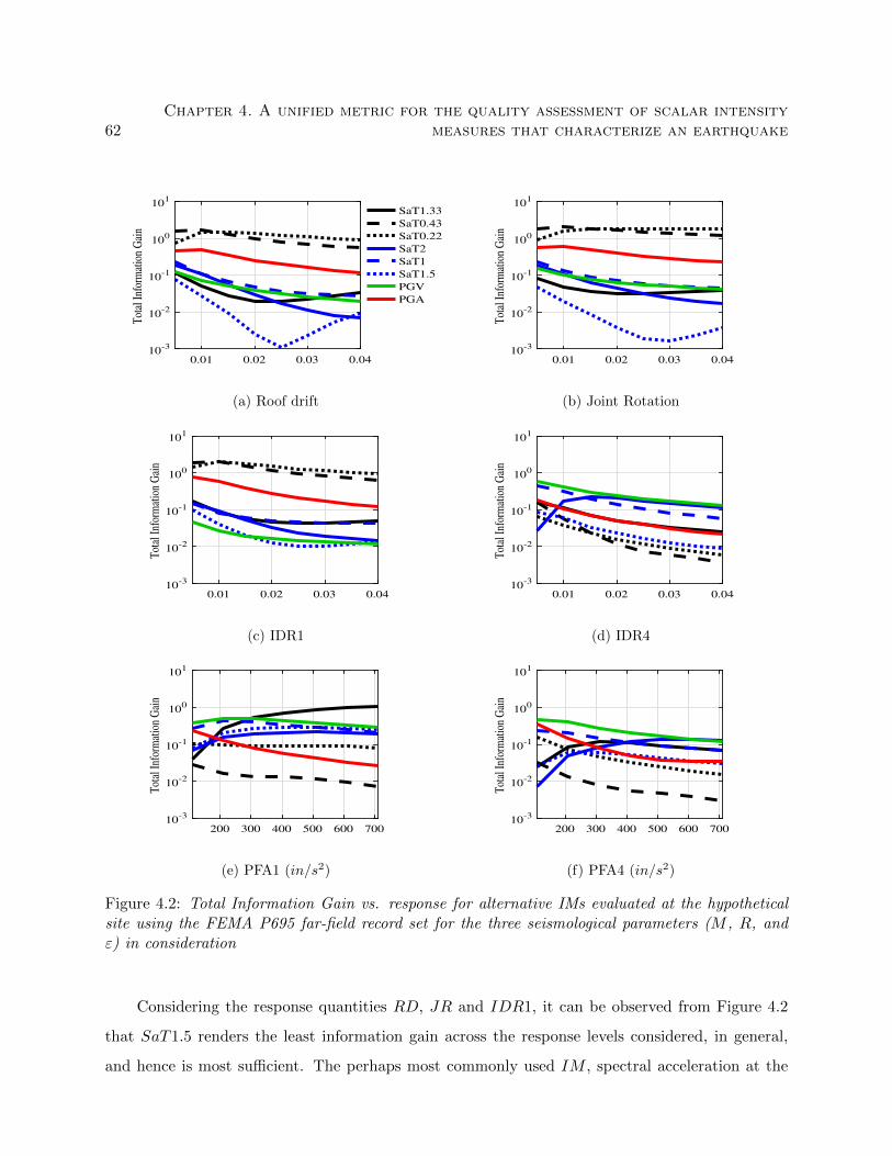
62Chapter 4. A unified metric for the quality assessment of scalar intensity
measures that characterize an earthquake
0.01 0.02 0.03 0.04
10-3
10-2
10-1
100
101
To
tal
Info
rmati
on
Gain
SaT1.33
SaT0.43
SaT0.22
SaT2
SaT1
SaT1.5
PGV
PGA
(a) Roof drift
0.01 0.02 0.03 0.04
10-3
10-2
10-1
100
101
Tota
l In
form
ati
on G
ain
(b) Joint Rotation
0.01 0.02 0.03 0.04
10-3
10-2
10-1
100
101
Tota
l In
form
ati
on G
ain
(c) IDR1
0.01 0.02 0.03 0.04
10-3
10-2
10-1
100
101
Tota
l In
form
ati
on G
ain
(d) IDR4
200 300 400 500 600 700
10-3
10-2
10-1
100
101
Tota
l In
form
ati
on G
ain
(e) PFA1 (in/s2)
200 300 400 500 600 700
10-3
10-2
10-1
100
101
Tota
l In
form
ati
on G
ain
(f) PFA4 (in/s2)
Figure 4.2: Total Information Gain vs. response for alternative IMs evaluated at the hypotheticalsite using the FEMA P695 far-field record set for the three seismological parameters (M , R, andε) in consideration
Considering the response quantities RD, JR and IDR1, it can be observed from Figure 4.2
that SaT1.5 renders the least information gain across the response levels considered, in general,
and hence is most sufficient. The perhaps most commonly used IM , spectral acceleration at the
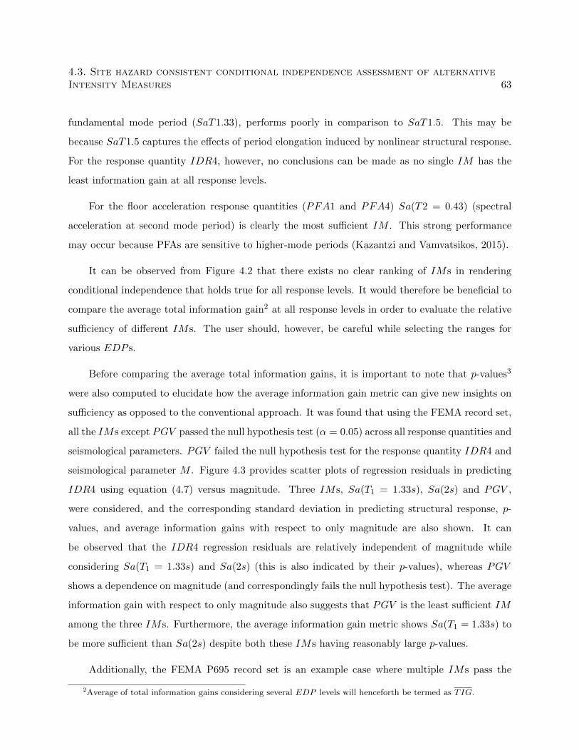
4.3. Site hazard consistent conditional independence assessment of alternativeIntensity Measures 63
fundamental mode period (SaT1.33), performs poorly in comparison to SaT1.5. This may be
because SaT1.5 captures the effects of period elongation induced by nonlinear structural response.
For the response quantity IDR4, however, no conclusions can be made as no single IM has the
least information gain at all response levels.
For the floor acceleration response quantities (PFA1 and PFA4) Sa(T2 = 0.43) (spectral
acceleration at second mode period) is clearly the most sufficient IM . This strong performance
may occur because PFAs are sensitive to higher-mode periods (Kazantzi and Vamvatsikos, 2015).
It can be observed from Figure 4.2 that there exists no clear ranking of IMs in rendering
conditional independence that holds true for all response levels. It would therefore be beneficial to
compare the average total information gain2 at all response levels in order to evaluate the relative
sufficiency of different IMs. The user should, however, be careful while selecting the ranges for
various EDP s.
Before comparing the average total information gains, it is important to note that p-values3
were also computed to elucidate how the average information gain metric can give new insights on
sufficiency as opposed to the conventional approach. It was found that using the FEMA record set,
all the IMs except PGV passed the null hypothesis test (α = 0.05) across all response quantities and
seismological parameters. PGV failed the null hypothesis test for the response quantity IDR4 and
seismological parameter M . Figure 4.3 provides scatter plots of regression residuals in predicting
IDR4 using equation (4.7) versus magnitude. Three IMs, Sa(T1 = 1.33s), Sa(2s) and PGV ,
were considered, and the corresponding standard deviation in predicting structural response, p-
values, and average information gains with respect to only magnitude are also shown. It can
be observed that the IDR4 regression residuals are relatively independent of magnitude while
considering Sa(T1 = 1.33s) and Sa(2s) (this is also indicated by their p-values), whereas PGV
shows a dependence on magnitude (and correspondingly fails the null hypothesis test). The average
information gain with respect to only magnitude also suggests that PGV is the least sufficient IM
among the three IMs. Furthermore, the average information gain metric shows Sa(T1 = 1.33s) to
be more sufficient than Sa(2s) despite both these IMs having reasonably large p-values.
Additionally, the FEMA P695 record set is an example case where multiple IMs pass the
2Average of total information gains considering several EDP levels will henceforth be termed as TIG.
64Chapter 4. A unified metric for the quality assessment of scalar intensity
measures that characterize an earthquake
null hypothesis test, making it difficult to find the degree to which different IMs are rendering
conditional independence. In such cases, the average information gain metric not only reduces the
multiple criteria of p-values with respect to different seismological parameter to a single criteria,
but also facilitates sufficiency comparison across a suite of IMs, response quantities and record
sets.
6.5 6.9 7.3 7.7
Earthquake magnitude, M
-1
-0.5
0
0.5
1
Resi
duals
, ǫ
IDR
4 | S
a(T
1 =
1.3
3s)
β = 0.27, p = 0.63, IGM
= 0.017
(a) Sa(T1 = 1.33s)
6.5 6.9 7.3 7.7
Earthquake magnitude, M
-1
-0.5
0
0.5
1R
esid
uals
, ǫ
IDR
4 | S
a(2
s)
β = 0.31, p = 0.51, IGM
= 0.061
(b) Sa(2s)
6.5 6.9 7.3 7.7
Earthquake magnitude, M
-1
-0.5
0
0.5
1
Resi
duals
, ǫ
IDR
4 | P
GV
β = 0.28, p = 0.03, IGM
= 0.25
(c) PGV
Figure 4.3: IDR4 regression residuals versus M under the FEMA P695 far-field record set for IMs(a) Sa(T1 = 1.33s), (b) Sa(2s), and (c) PGV . Standard deviation in lnEDP given lnIM (denotedas β in this figure), p-value and Information Gain with respect to M are depicted.
The average information gains across different response levels for different response quantities
for the suite of IMs considered in this study under the FEMA record set are shown in Table 4.1
(under the heading “Exact deaggregation”). It can be observed that, in general, for the response
quantities RD, JR, IDR1 and IDR4 the extended mode period spectral acceleration, Sa(1.5s),
is the most sufficient. For the response quantities PFA1 and PFA4, on the other hand, Sa(T2 =
0.43s) is the most sufficient. These generally most sufficient IMs are highlighted in blue in Table
4.1.
4.3.5 IM conditional independence assessment using approximate deaggrega-
tion
Although the IM sufficiency assessment procedure described in section 4.3.4 has many advantages,
it requires continuous deaggregation information at very fine IM intervals. Hence the practical
application of this procedure can be cumbersome, motivating an approach to approximate deaggre-
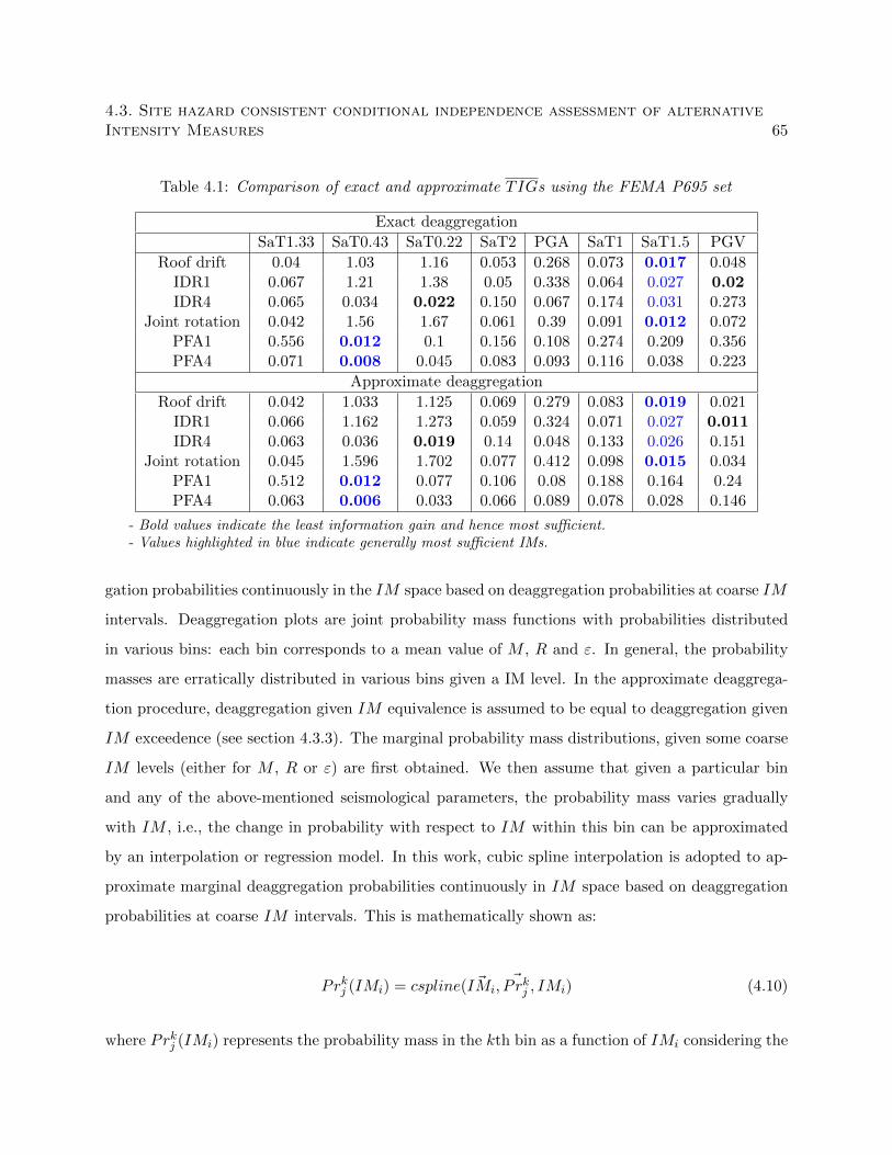
4.3. Site hazard consistent conditional independence assessment of alternativeIntensity Measures 65
Table 4.1: Comparison of exact and approximate TIGs using the FEMA P695 set
Exact deaggregation
SaT1.33 SaT0.43 SaT0.22 SaT2 PGA SaT1 SaT1.5 PGV
Roof drift 0.04 1.03 1.16 0.053 0.268 0.073 0.017 0.048IDR1 0.067 1.21 1.38 0.05 0.338 0.064 0.027 0.02IDR4 0.065 0.034 0.022 0.150 0.067 0.174 0.031 0.273
Joint rotation 0.042 1.56 1.67 0.061 0.39 0.091 0.012 0.072PFA1 0.556 0.012 0.1 0.156 0.108 0.274 0.209 0.356PFA4 0.071 0.008 0.045 0.083 0.093 0.116 0.038 0.223
Approximate deaggregation
Roof drift 0.042 1.033 1.125 0.069 0.279 0.083 0.019 0.021IDR1 0.066 1.162 1.273 0.059 0.324 0.071 0.027 0.011IDR4 0.063 0.036 0.019 0.14 0.048 0.133 0.026 0.151
Joint rotation 0.045 1.596 1.702 0.077 0.412 0.098 0.015 0.034PFA1 0.512 0.012 0.077 0.106 0.08 0.188 0.164 0.24PFA4 0.063 0.006 0.033 0.066 0.089 0.078 0.028 0.146
- Bold values indicate the least information gain and hence most sufficient.- Values highlighted in blue indicate generally most sufficient IMs.
gation probabilities continuously in the IM space based on deaggregation probabilities at coarse IM
intervals. Deaggregation plots are joint probability mass functions with probabilities distributed
in various bins: each bin corresponds to a mean value of M , R and ε. In general, the probability
masses are erratically distributed in various bins given a IM level. In the approximate deaggrega-
tion procedure, deaggregation given IM equivalence is assumed to be equal to deaggregation given
IM exceedence (see section 4.3.3). The marginal probability mass distributions, given some coarse
IM levels (either for M , R or ε) are first obtained. We then assume that given a particular bin
and any of the above-mentioned seismological parameters, the probability mass varies gradually
with IM , i.e., the change in probability with respect to IM within this bin can be approximated
by an interpolation or regression model. In this work, cubic spline interpolation is adopted to ap-
proximate marginal deaggregation probabilities continuously in IM space based on deaggregation
probabilities at coarse IM intervals. This is mathematically shown as:
Prkj (IMi) = cspline( ~IMi,~Prkj , IMi) (4.10)
where Prkj (IMi) represents the probability mass in the kth bin as a function of IMi considering the
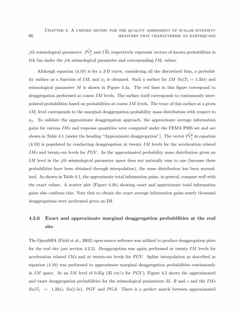
66Chapter 4. A unified metric for the quality assessment of scalar intensity
measures that characterize an earthquake
jth seismological parameter. ~Prkj and ~IMi respectively represent vectors of known probabilities in
kth bin under the jth seismological parameter and corresponding IMi values.
Although equation (4.10) is for a 2-D curve, considering all the discretized bins, a probabil-
ity surface as a function of IMi and φj is obtained. Such a surface for IM Sa(T1 = 1.33s) and
seismological parameter M is shown in Figure 4.4a. The red lines in this figure correspond to
deaggregation performed at coarse IM levels. The surface itself corresponds to continuously inter-
polated probabilities based on probabilities at coarse IM levels. The trace of this surface at a given
IMi level corresponds to the marginal deaggregation probability mass distribution with respect to
φj . To validate the approximate deaggregation approach, the approximate average information
gains for various IMs and response quantities were computed under the FEMA P695 set and are
shown in Table 4.1 (under the heading “Approximate deaggregation”). The vector ~Prkj in equation
(4.10) is populated by conducting deaggregation at twenty IM levels for the acceleration related
IMs and twenty-six levels for PGV . As the approximated probability mass distribution given an
IM level in the jth seismological parameter space does not naturally sum to one (because these
probabilities have been obtained through interpolation), the mass distribution has been normal-
ized. As shown in Table 4.1, the approximate total information gains, in general, compare well with
the exact values. A scatter plot (Figure 4.4b) showing exact and approximate total information
gains also confirms this. Note that to obtain the exact average information gains nearly thousand
deaggregations were performed given an IM.
4.3.6 Exact and approximate marginal deaggregation probabilities at the real
site
The OpenSHA (Field et al., 2003) open-source software was utilized to produce deaggregation plots
for the real site (see section 4.2.3). Deaggregation was again performed at twenty IM levels for
acceleration related IMs and at twenty-six levels for PGV . Spline interpolation as described in
equation (4.10) was performed to approximate marginal deaggregation probabilities continuously
in IM space. At an IM level of 0.35g (35 cm/s for PGV ), Figure 4.5 shows the approximated
and exact deaggregation probabilities for the seismological parameters M , R and ε and the IMs
Sa(T1 = 1.33s), Sa(1.5s), PGV and PGA. There is a perfect match between approximated
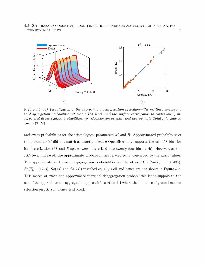
4.3. Site hazard consistent conditional independence assessment of alternativeIntensity Measures 67
Sa(T1 = 1.33s)
2
1
04
M
6
8
0
0.1
0.2
% c
ontr
ibut
ion
to λ
(IM
)
Approximate
Exact
(a)
0 0.6 1.2 1.8
Approx. TIG
0
0.6
1.2
1.8
Exac
t T
IG
R2 = 0.994
(b)
Figure 4.4: (a) Visualization of the approximate deaggregation procedure—the red lines correspondto deaggregation probabilities at coarse IM levels and the surface corresponds to continuously in-terpolated deaggregation probabilities; (b) Comparison of exact and approximate Total InformationGains (TIG).
and exact probabilities for the seismological parameters M and R. Approximated probabilities of
the parameter ‘ε’ did not match as exactly because OpenSHA only supports the use of 8 bins for
its discretization (M and R spaces were discretized into twenty-four bins each). However, as the
IMi level increased, the approximate probababilities related to ‘ε’ converged to the exact values.
The approximate and exact deaggregation probabilities for the other IMs (Sa(T2 = 0.43s),
Sa(T3 = 0.22s), Sa(1s) and Sa(2s)) matched equally well and hence are not shown in Figure 4.5.
This match of exact and approximate marginal deaggregation probabilities lends support to the
use of the approximate deaggregation approach in section 4.4 where the influence of ground motion
selection on IM sufficiency is studied.
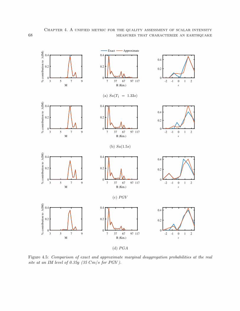
68Chapter 4. A unified metric for the quality assessment of scalar intensity
measures that characterize an earthquake
3 5 7 9
M
0
0.2
0.4
% c
on
trib
uti
on
to
λ
(IM
)
7 37 67 97 117
R (Km.)
0
0.2
0.4
Exact Approximate
-2 -1 0 1 2
ǫ
0
0.2
0.4
(a) Sa(T1 = 1.33s)
3 5 7 9
M
0
0.2
0.4
% c
on
trib
uti
on
to
λ
(IM
)
7 37 67 97 117
R (Km.)
0
0.2
0.4
-2 -1 0 1 2
ǫ
0
0.2
0.4
(b) Sa(1.5s)
3 5 7 9
M
0
0.2
0.4
% c
on
trib
uti
on
to
λ
(IM
)
7 37 67 97 117
R (Km.)
0
0.2
0.4
-2 -1 0 1 2
ǫ
0
0.2
0.4
(c) PGV
3 5 7 9
M
0
0.2
0.4
% c
on
trib
uti
on
to
λ
(IM
)
7 37 67 97 117
R (Km.)
0
0.2
0.4
-2 -1 0 1 2
ǫ
0
0.2
0.4
(d) PGA
Figure 4.5: Comparison of exact and approximate marginal deaggregation probabilities at the realsite at an IM level of 0.35g (35 Cm/s for PGV ).
4.4. Influence of ground motion record sets on sufficiency of scalar IMs 69
4.4 Influence of ground motion record sets on sufficiency of scalar
IMs
RD IDR1 IDR4 JR PFA1 PFA40
0.5
1
1.5
2
TIG
(bits)
Sa(1.5s)
Sa(1.5s)
Sa(0.22s)
Sa(1.5s)
PGA
Sa(0.43s)
Sa(T1 = 1.33s)
Sa(T2 = 0.43s)
Sa(T3 = 0.22s)
Sa(2s)
Sa(1s)
Sa(1.5s)
PGV
PGA
(a)
RD IDR1 IDR4 JR PFA1 PFA4
0
0.5
1
1.5
2
TIG
(bits)
PGA
PGA
PGA
PGA
Sa(2s) Sa(0.43s)
(b)
RD IDR1 IDR4 JR PFA1 PFA4
0
0.5
1
1.5
2
TIG
(bits)
Sa(2s)
Sa(2s)
PGV
Sa(1.5s)
Sa(0.43s)
Sa(0.43s)
(c)
RD IDR1 IDR4 JR PFA1 PFA4
0
0.5
1
1.5
2
TIG
(bits)
Sa(2s)
Sa(1.5s)
Sa(1s)
Sa(2s)
PGA
PGA
(d)
Figure 4.6: Influence of ground motion selection on sufficiency: TIGs for various IMs at the realsite considering the record set (a) FEMA P695 far-field (b) Medina-Krawinkler LMSR-N (c) CSmatched (no pulse) (d) CS matched (pulse). The most sufficient IMs (least TIG) for variousEDP -record set combinations are stated above each EDP . In (c), the IM Sa(2s) has a TIG of2.08 and 2.28 bits for PFA1 and PFA4, respectively.
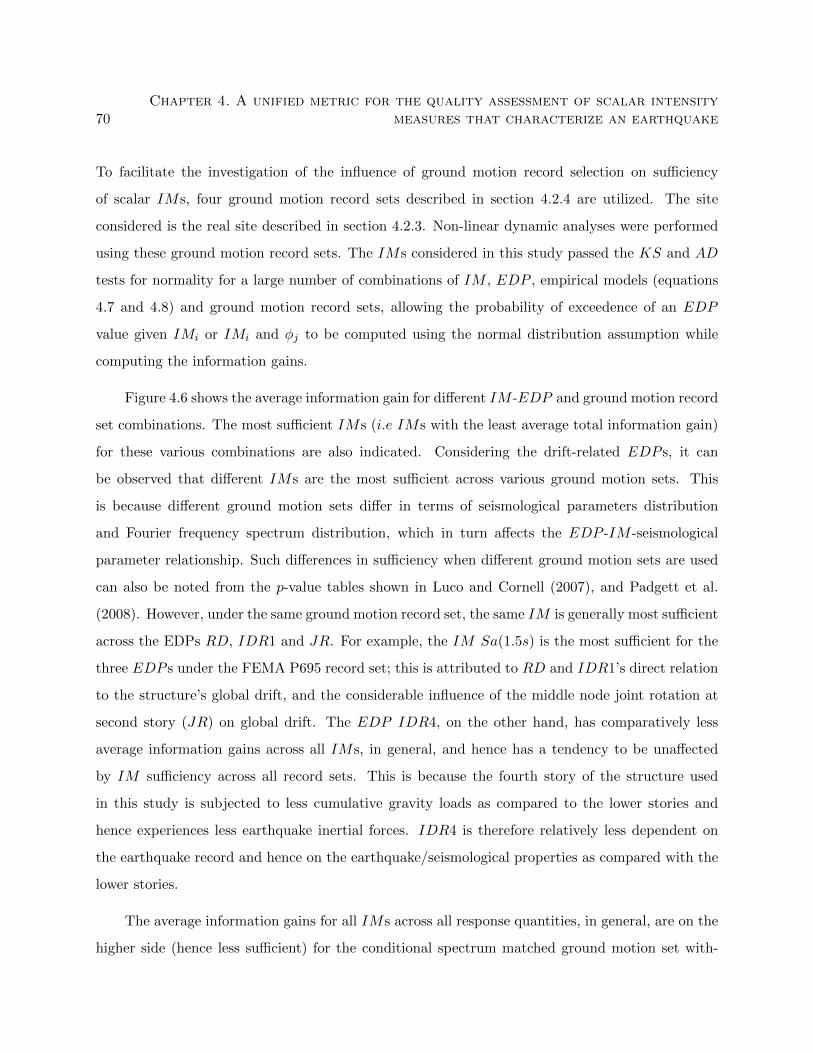
70Chapter 4. A unified metric for the quality assessment of scalar intensity
measures that characterize an earthquake
To facilitate the investigation of the influence of ground motion record selection on sufficiency
of scalar IMs, four ground motion record sets described in section 4.2.4 are utilized. The site
considered is the real site described in section 4.2.3. Non-linear dynamic analyses were performed
using these ground motion record sets. The IMs considered in this study passed the KS and AD
tests for normality for a large number of combinations of IM , EDP , empirical models (equations
4.7 and 4.8) and ground motion record sets, allowing the probability of exceedence of an EDP
value given IMi or IMi and φj to be computed using the normal distribution assumption while
computing the information gains.
Figure 4.6 shows the average information gain for different IM -EDP and ground motion record
set combinations. The most sufficient IMs (i.e IMs with the least average total information gain)
for these various combinations are also indicated. Considering the drift-related EDP s, it can
be observed that different IMs are the most sufficient across various ground motion sets. This
is because different ground motion sets differ in terms of seismological parameters distribution
and Fourier frequency spectrum distribution, which in turn affects the EDP -IM -seismological
parameter relationship. Such differences in sufficiency when different ground motion sets are used
can also be noted from the p-value tables shown in Luco and Cornell (2007), and Padgett et al.
(2008). However, under the same ground motion record set, the same IM is generally most sufficient
across the EDPs RD, IDR1 and JR. For example, the IM Sa(1.5s) is the most sufficient for the
three EDP s under the FEMA P695 record set; this is attributed to RD and IDR1’s direct relation
to the structure’s global drift, and the considerable influence of the middle node joint rotation at
second story (JR) on global drift. The EDP IDR4, on the other hand, has comparatively less
average information gains across all IMs, in general, and hence has a tendency to be unaffected
by IM sufficiency across all record sets. This is because the fourth story of the structure used
in this study is subjected to less cumulative gravity loads as compared to the lower stories and
hence experiences less earthquake inertial forces. IDR4 is therefore relatively less dependent on
the earthquake record and hence on the earthquake/seismological properties as compared with the
lower stories.
The average information gains for all IMs across all response quantities, in general, are on the
higher side (hence less sufficient) for the conditional spectrum matched ground motion set with-
4.4. Influence of ground motion record sets on sufficiency of scalar IMs 71
out pulse-like ground motions. For the conditional spectrum matched pulse-like ground motions,
however, it can be seen that the average information gains tend to be on the lower side. The IM
PGV has a tendency to have low total information gain values, if not the least, across all the drift
related EDP s. This is mainly because, unlike ordinary ground motions, pulse-like ground motions
are characterized by their distinct velocity pulses (Baker, 2007b) which can be better accounted
for by the scalar IM PGV . However, it is interesting to note that PGV is not among the most
efficient IMs for drift related EDP s under the pulse-like record set.
Floor accelerations are important EDP s in that they have a direct impact on damage to non-
structural components and contents in a building. Results indicate that for the floor acceleration
related EDP s (PFA1 and PFA4), either Sa(T2 = 0.43s) or PGA tend to be most sufficient across
all record sets in general. It is also interesting to note that these IMs, Sa(T2 = 0.43s) and PGA,
also tend to be the most efficient (i.e., less standard deviation) in predicting the floor acceleration
related EDP s.
The total information gains presented in Figure 4.6 directly represent the differences in f(IMi|EDP >
y) distributions without and with the various seismological parameters. For instance, Figure 4.7
shows Sa(T1 = 1.33s) given Roof Drift > 0.04 density distributions for the CS matched no pulse
and CS matched pulse sets. For this roof drift level, it can be seen that Sa(T1 = 1.33s) distributions
without and with the seismological parameters differ considerably for the CS matched no pulse set.
For the CS matched pulse set on the other hand, these density distributions are seen to be con-
sistent. The average of total information gains also shown in Figure 4.7 reflect these differences in
density distributions.
Discussion on demand hazard estimation
The demand hazard curve when a seismological parameter and IMi are considered can be calculated
using:
λ(EDP > y) =
∫IMi
P r(EDP > y|IMi) |dλ(IMi)
dIMi|dIMi (4.11)
72Chapter 4. A unified metric for the quality assessment of scalar intensity
measures that characterize an earthquake
0 1 2 3 4 5
IMi = Sa(T1 = 1.33s) (g)
0
0.5
1
1.5
f(IM
i|RD
>0.04)
T IG = 0.11
Only IM
IM and M
IM and R
IM and ǫ
(a)
0 1 2 3 4 5
IMi = Sa(T1 = 1.33s) (g)
0
0.5
1
1.5
f(IM
i|RD
>0.04)
T IG = 0.03
(b)
Figure 4.7: Sa(T1 = 1.33s) given Roof Drift > 0.04 distributions without and with consideringthe seismological parameters (M , R, ε) for the record sets: (a) CS matched no pulse set; (b) CSmatched pulse set. The TIGs are also depicted.
where P r(EDP > y|IMi) is the demand fragility computed using equation (4.2) while considering a
seismological parameter. The demand hazard curve when only IMi is considered can be computed
by replacing P r(EDP > y|IMi) in the above equation with Pr(EDP > y|IMi) (equation 4.1). In
this section we explore how Total Information Gain (TIG) reflects changes on the demand hazard
curve when seismological parameters are considered.
This study adopted 192 combinations of EDP s, IMs and ground motion sets. Across all
these combinations, it was found that TIG generally represented changes in demand hazards when
seismological parameters are considered in computations. Figures 4.8 and 4.9 show demand hazards
for different EDP -IM -record set combinations computed without and with considering M , R
and ε. TIGs and the standard deviations of the prediction of EDP given IMi (βlnEDP |lnIMi)
are also shown. From these figures, the following observations can be made: (i) For the same
EDP , different IM -record set combinations give different estimates of demand hazards. This
signifies the importance of proper ground motion and IM selection also emphasized in various
other studies. (ii) For the various combinations, different seismological parameters have a different
effect on the demand hazard across the EDP levels (comparing with the ‘only IM ’ curve). For
4.4. Influence of ground motion record sets on sufficiency of scalar IMs 73
some combinations, seismological parameters cause an increment in demand hazard at high EDP
levels (Figure 4.9d IM and ε curve), while for others, these seismological parameters cause a
reduction in hazard at low EDP levels (Figure 4.8a IM and M curve). In some cases, seismological
parameters have a mixed effect on the demand hazard; increasing the hazard at some EDP levels
while reducing the hazard at other levels (Figure 4.8d IM and ε curve). This makes inferring the
influence of seismological parameters by directly comparing differences in demand hazards from
the ‘only IM ’ curve a difficult task. (iii) The TIGs are seen to represent changes in demand
hazards when seismological parameters are included. Low values of TIG indicate consistency
between demand hazards with and without including seismological parameters (example: Figure
4.8b). Intermediate values of TIG show noticeable changes in demand hazards from the ‘only IM ’
curve (examples: Figures 4.8c, 4.9d and 4.9f), while high values of TIG suggest that including
seismological parameters individually lead to considerable deviations from the ‘only IM ’ curve
(examples: Figures 4.8a, 4.9b and 4.9e). We also note that in general large changes in TIG imply
proportionally large changes in demand hazard, but this is not always the case.
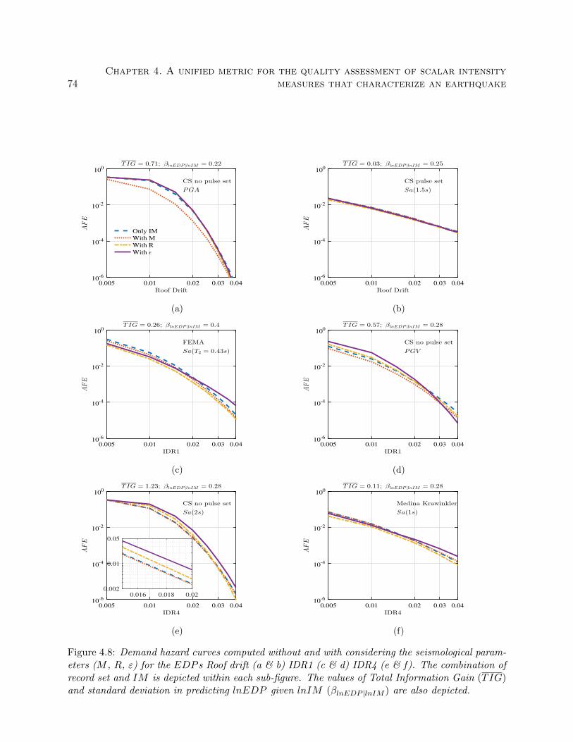
74Chapter 4. A unified metric for the quality assessment of scalar intensity
measures that characterize an earthquake
0.005 0.01 0.02 0.03 0.04
Roof Drift
10-6
10-4
10-2
100
AFE
T IG = 0.71; βlnEDP |lnIM = 0.22
CS no pulse set
PGA
Only IM
With M
With R
With ǫ
(a)
0.005 0.01 0.02 0.03 0.04
Roof Drift
10-6
10-4
10-2
100
AFE
T IG = 0.03; βlnEDP |lnIM = 0.25
CS pulse set
Sa(1.5s)
(b)
0.005 0.01 0.02 0.03 0.04
IDR1
10-6
10-4
10-2
100
AFE
T IG = 0.26; βlnEDP |lnIM = 0.4
FEMA
Sa(T2 = 0.43s)
(c)
0.005 0.01 0.02 0.03 0.04
IDR1
10-6
10-4
10-2
100
AFE
T IG = 0.57; βlnEDP |lnIM = 0.28
CS no pulse set
PGV
(d)
0.005 0.01 0.02 0.03 0.04
IDR4
10-6
10-4
10-2
100
AFE
T IG = 1.23; βlnEDP |lnIM = 0.28
CS no pulse set
Sa(2s)
0.016 0.018 0.02
0.002
0.01
0.05
(e)
0.005 0.01 0.02 0.03 0.04
IDR4
10-6
10-4
10-2
100
AFE
T IG = 0.11; βlnEDP |lnIM = 0.28
Medina Krawinkler
Sa(1s)
(f)
Figure 4.8: Demand hazard curves computed without and with considering the seismological param-eters (M , R, ε) for the EDP s Roof drift (a & b) IDR1 (c & d) IDR4 (e & f). The combination ofrecord set and IM is depicted within each sub-figure. The values of Total Information Gain (TIG)and standard deviation in predicting lnEDP given lnIM (βlnEDP |lnIM ) are also depicted.
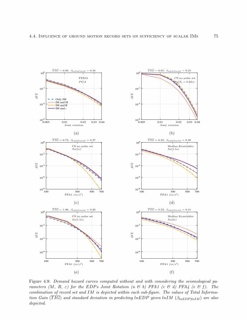
4.4. Influence of ground motion record sets on sufficiency of scalar IMs 75
0.005 0.01 0.02 0.03 0.04
Joint rotation
10-6
10-4
10-2
100
AFE
T IG = 0.08; βlnEDP |lnIM = 0.48
FEMA
PGA
Only IM
IM and M
IM and R
IM and ǫ
(a)
0.005 0.01 0.02 0.03 0.04
Joint rotation
10-6
10-4
10-2
100
AFE
T IG = 0.85; βlnEDP |lnIM = 0.25
CS no pulse set
Sa(T3 = 0.22s)
(b)
100 300 500 700
PFA1 (in/s2)
10-8
10-6
10-4
10-2
100
AFE
T IG = 0.72; βlnEDP |lnIM = 0.37
CS no pulse setSa(1s)
(c)
100 300 500 700
PFA1 (in/s2)
10-8
10-6
10-4
10-2
100
AFE
T IG = 0.32; βlnEDP |lnIM = 0.38
Medina KrawinklerSa(1.5s)
(d)
100 300 500 700
PFA1 (in/s2)
10-6
10-4
10-2
100
AFE
T IG = 1.06; βlnEDP |lnIM = 0.26
CS no pulse set
Sa(1.5s)
(e)
100 300 500 700
PFA1 (in/s2)
10-6
10-4
10-2
100
AFE
T IG = 0.33; βlnEDP |lnIM = 0.41
Medina Krawinkler
Sa(2s)
(f)
Figure 4.9: Demand hazard curves computed without and with considering the seismological pa-rameters (M , R, ε) for the EDP s Joint Rotation (a & b) PFA1 (c & d) PFA4 (e & f). Thecombination of record set and IM is depicted within each sub-figure. The values of Total Informa-tion Gain (TIG) and standard deviation in predicting lnEDP given lnIM (βlnEDP |lnIM ) are alsodepicted.

76Chapter 4. A unified metric for the quality assessment of scalar intensity
measures that characterize an earthquake
If other seismological parameters in a Ground Motion Prediction Model (GMPM), such as M2,
M ∗ lnR or lnV s30, are considered, the (TIG) values increase. In addition, if all the seismological
parameters are considered at once while linking EDP and IM , the resulting demand hazard curve
may be very different from the curve obtained using only IM . The finite datasets used, however,
limits us to treating each parameter in a GMPM individually.
The proposed methodology to quantify sufficiency can be an aid for ground motion selection.
For example, for the CS matched ground motions, it can be noted from Figures 4.6c and 4.6d that
the TIGs for drift related EDP s are low when the IM is Sa(T1 = 1.33s) (spectral acceleration at
which the CS is conditioned; structure’s fundamental time period). This may suggest considering a
CS approach for ground motion selection and Sa(T1) as the IM to avoid problems with insufficiency
for these classes of structures. However, it is interesting to note that for the CS matched no pulse
set, IMs other than Sa(T1) may render high values of TIG. The sufficiency of different IMs
considering CS matched ground motions at various conditioning periods, in particular, is a topic
for future research.
4.5 Relation between the sufficiency and the efficiency criterion
of seismic IMs and their unification
The relation between βlnEDP |lnIM , which is a measure for efficiency of an IM , and TIG, which
is measure for sufficiency of an IM , is explored in this section. A scatter plot of ln(TIG) versus
ln(βlnEDP |lnIM ) considering all EDP -IM -ground motion set combinations adopted in this study is
shown in Figure 4.10. The median prediction , standard deviation of this prediction, and Pearson
correlation coefficient are also shown. It can be observed from this figure that there is considerable
scatter around the median prediction, indicating that efficiency and sufficiency of an IM are weakly
correlated. This is also implied by the Pearson correlation coefficient, which is 0.29. However,
there is a positive correlation between efficiency and sufficiency indicating as an IM becomes more
efficient the same IM also tends to become more sufficient on an average. This observation is in line
with the general intuition that efficiency of an IM determines the level of sufficiency of that IM .
The case-specific validity of this intuition, however, must be questioned due to the large scatter
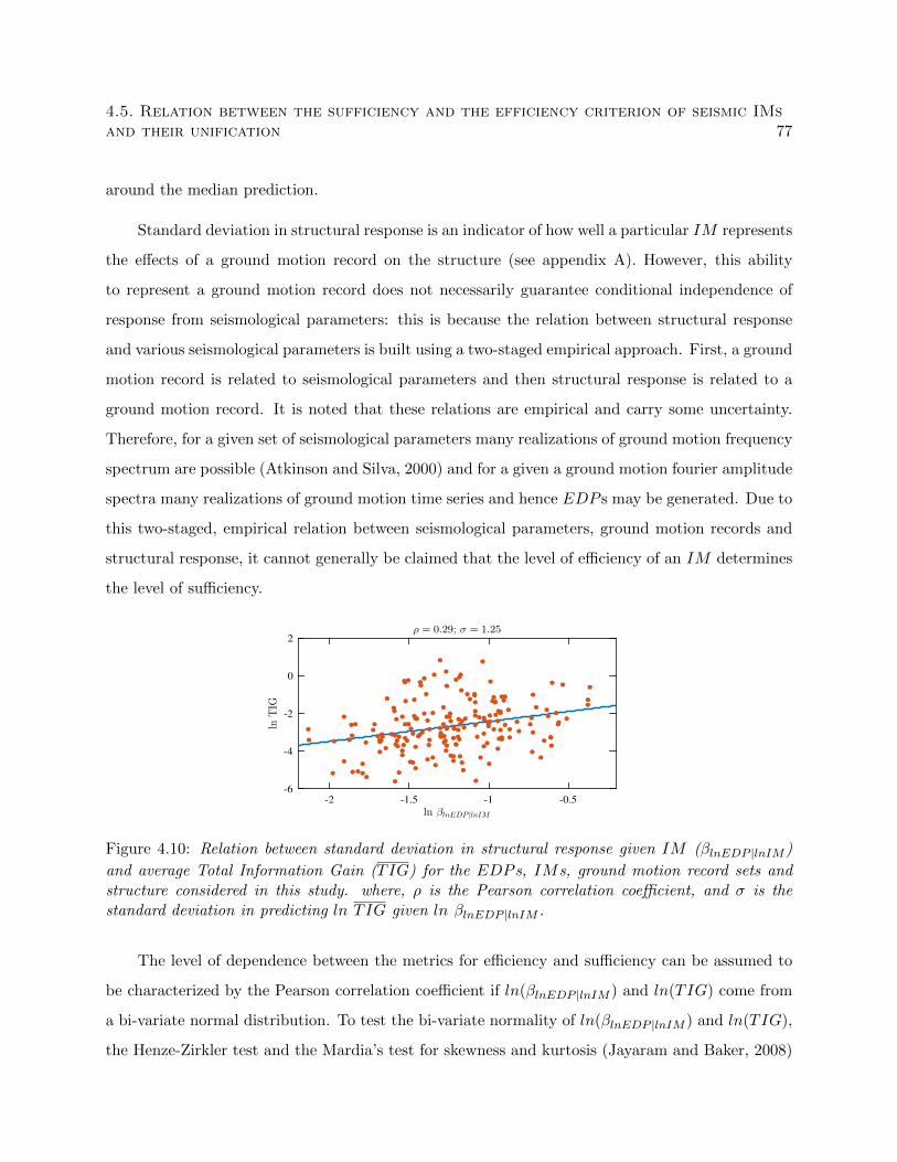
4.5. Relation between the sufficiency and the efficiency criterion of seismic IMsand their unification 77
around the median prediction.
Standard deviation in structural response is an indicator of how well a particular IM represents
the effects of a ground motion record on the structure (see appendix A). However, this ability
to represent a ground motion record does not necessarily guarantee conditional independence of
response from seismological parameters: this is because the relation between structural response
and various seismological parameters is built using a two-staged empirical approach. First, a ground
motion record is related to seismological parameters and then structural response is related to a
ground motion record. It is noted that these relations are empirical and carry some uncertainty.
Therefore, for a given set of seismological parameters many realizations of ground motion frequency
spectrum are possible (Atkinson and Silva, 2000) and for a given a ground motion fourier amplitude
spectra many realizations of ground motion time series and hence EDP s may be generated. Due to
this two-staged, empirical relation between seismological parameters, ground motion records and
structural response, it cannot generally be claimed that the level of efficiency of an IM determines
the level of sufficiency.
-2 -1.5 -1 -0.5
ln βlnEDP |lnIM
-6
-4
-2
0
2
lnTIG
ρ = 0.29; σ = 1.25
Figure 4.10: Relation between standard deviation in structural response given IM (βlnEDP |lnIM )
and average Total Information Gain (TIG) for the EDP s, IMs, ground motion record sets andstructure considered in this study. where, ρ is the Pearson correlation coefficient, and σ is thestandard deviation in predicting ln TIG given ln βlnEDP |lnIM .
The level of dependence between the metrics for efficiency and sufficiency can be assumed to
be characterized by the Pearson correlation coefficient if ln(βlnEDP |lnIM ) and ln(TIG) come from
a bi-variate normal distribution. To test the bi-variate normality of ln(βlnEDP |lnIM ) and ln(TIG),
the Henze-Zirkler test and the Mardia’s test for skewness and kurtosis (Jayaram and Baker, 2008)
78Chapter 4. A unified metric for the quality assessment of scalar intensity
measures that characterize an earthquake
were performed. All three tests fail to reject the null hypothesis that ln(βlnEDP |lnIM ) and ln(TIG)
come from a bi-variate normal distribution at a significance level of 0.05. The p-value for the
Henze-Zirkler test is 0.19 and the p-values for the Mardia’s test are 0.17 and 0.18 for skewness and
kurtosis respectively. Given that these two metrics for efficiency and sufficiency (ln(βlnEDP |lnIM )
and ln(TIG)) are bi-variate normal, and their Pearson’s correlation coefficient is low (ρ = 0.29),
these metrics can be considered to have low statistical dependence. This conclusion may be useful
to support derivation of a unified metric for both efficiency and sufficiency.
Proposal for a unified metric to gauge the efficiency and sufficiency of a scalar IM
The natural logarithm of metrics for efficiency and sufficiency, βlnEDP |lnIM and TIG, are correlated
to some degree and are not on the same scale. First, a Mahalanobis transformation (or a standard
normal transformation; Vidakovic 2011) is utilized to de-correlate and transform ln βlnEDP |lnIM
and ln TIG into a bi-variate standard normal space. This transformation can be performed using:
~Zi = S−1/2 ( ~Xi − ~XM
)(4.12)
where ~Zi is a 2 × 1 vector containing transformed values, S is the covariance matrix, ~Xi is a
2 × 1 vector containing the original values and ~XM is a 2 × 1 vector containing the mean values
of ln βlnEDP |lnIM and ln TIG. A scatter plot of the transformed values is shown in Figure 4.11a.
Now, theoretically, the co-ordinates of the “perfect” IM in this transformed space would tend to
(−∞,+∞). Or in other words, this perfect IM would have co-ordinates tending to (0, 0) in the
exponent of transformed space. A scatter plot of the exponent of vector ~Zi is shown in Figure
4.11b. The Euclidean norm of the vector exp( ~Zi) is a measure of how efficient and sufficient an IM
is. The definition of this unified metric is mathematically given by:
Ai = ln(||exp( ~Zi)||
)(4.13)
where ||.|| represents the Euclidean norm (distance). In the above equation, natural logarithm is
used for de-clustering purposes. The unified metric Ai is dimensionless and has bounds (−∞,+∞).
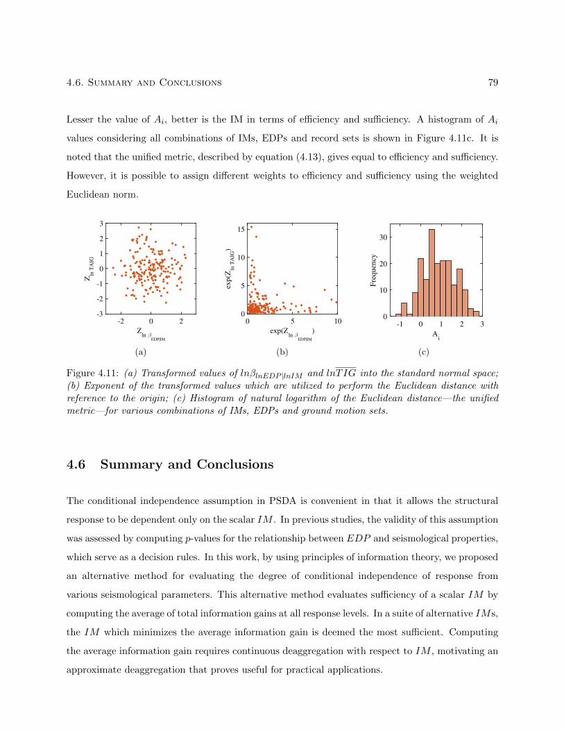
4.6. Summary and Conclusions 79
Lesser the value of Ai, better is the IM in terms of efficiency and sufficiency. A histogram of Ai
values considering all combinations of IMs, EDPs and record sets is shown in Figure 4.11c. It is
noted that the unified metric, described by equation (4.13), gives equal to efficiency and sufficiency.
However, it is possible to assign different weights to efficiency and sufficiency using the weighted
Euclidean norm.
Zln β
EDP|IM
-2 0 2
Zln
TA
IG
-3
-2
-1
0
1
2
3
(a)
exp(Zln β
EDP|IM
)
0 5 10
exp(Z
ln T
AIG
)
0
5
10
15
(b)
Ai
-1 0 1 2 3
Fre
qu
ency
0
10
20
30
(c)
Figure 4.11: (a) Transformed values of lnβlnEDP |lnIM and lnTIG into the standard normal space;(b) Exponent of the transformed values which are utilized to perform the Euclidean distance withreference to the origin; (c) Histogram of natural logarithm of the Euclidean distance—the unifiedmetric—for various combinations of IMs, EDPs and ground motion sets.
4.6 Summary and Conclusions
The conditional independence assumption in PSDA is convenient in that it allows the structural
response to be dependent only on the scalar IM . In previous studies, the validity of this assumption
was assessed by computing p-values for the relationship between EDP and seismological properties,
which serve as a decision rules. In this work, by using principles of information theory, we proposed
an alternative method for evaluating the degree of conditional independence of response from
various seismological parameters. This alternative method evaluates sufficiency of a scalar IM by
computing the average of total information gains at all response levels. In a suite of alternative IMs,
the IM which minimizes the average information gain is deemed the most sufficient. Computing
the average information gain requires continuous deaggregation with respect to IM , motivating an
approximate deaggregation that proves useful for practical applications.
80Chapter 4. A unified metric for the quality assessment of scalar intensity
measures that characterize an earthquake
The following conclusions are drawn:
• The proposed metric for IM sufficiency computes the total information gain by individually
adding the information gains due to the inclusion of different seismological parameters in
the regression model. Although this individual addition of information gains assumes that
the considered seismological parameters influence the structural response individually, this
operation avoided potential problems with multi-collinearity and inaccurate estimation of
regression co-efficients.
• The approximate deaggregation approach proposed here allowed for an accurate and practi-
cable estimation of the total information gain by reducing the number of deaggregations from
some hundreds to only about twenty per IM .
• We investigated the influence of ground motion record sets on the degree of sufficiency, and
found that for drift related EDP s, different IMs tended to be the most sufficient across
different record sets. This may be due to the differences in the properties of ground motion
record sets adopted. A common observation across all record sets was, however, given a record
set the same IM was generally most sufficient across the EDP s RD, IDR1 and JR. For
these EDP s under the conditional spectrum matched pulse-like ground motion set, the IM
PGV was found to have low values of total information gains. The EDP IDR4 was observed
to be relatively unaffected by IM sufficiency.
• For the floor acceleration related EDP s on the other hand, it was observed that the same
IMs were consistently most sufficient across all ground motion record sets.
• By evaluating the degree to which various IMs render conditional independence from seis-
mological parameters across four ground motion sets, we show that ground motion selection
can play an important role in IM sufficiency.
• The proposed total information gain metric generally represented changes in demand hazard
curves when seismological parameters are taken into consideration.
• Utilizing the metric for sufficiency and efficiency (TIGi and βEDP |IMi) it was observed that
the level of efficiency of an IM need not necessarily determine the IM ’s level of sufficiency.
4.6. Summary and Conclusions 81
• By conducting joint normality tests on natural logarithms of the metrics for sufficiency and
efficiency, we observed that these metrics come from a bi-variate normal distribution. We
also found that the level of dependence between the metrics for sufficiency and efficiency is
low indicated by a positive Pearson correlation coefficient of 0.29.
Sufficiency of a scalar IM is a very important condition in PSDA to avoid biased evaluation of
the seismic demand hazard: some authors refer to sufficiency as a sine qua non requirement for scalar
IMs (Kazantzi and Vamvatsikos, 2015). However, there has been no proper metric to quantify
the degree of sufficiency of alternative IMs. The p-value approach provides only a qualitative
rule for whether or not different seismological parameters influence the structural response. The
lack of a quantitative approach has hindered understanding of the interplay between efficiency and
sufficiency of IMs, with the selected ground motion record set being a primary element in governing
this relationship. It is expected that the total information gain metric proposed here will aid in
understanding this relation and can provide new insights, thus enabling the selection of a proper
scalar IM for a given site and application in PSDA.
Chapter 5
A pre-configured solution to the
problem of joint hazard estimation
given a suite of seismic intensity
measures
This chapter expands upon a study excerpted from:
Somayajulu L.N. Dhulipala, Adrian Rodriguez–Marek, and Madeleine M. Flint. “Computation
of vector hazard using salient features of seismic hazard deaggregation” Earthquake Spectra 2018
34(4) 1893-1912.
5.1 Introduction
Deaggregation is one of the products of Probabilistic Seismic Hazard Analysis (PSHA) that aids
in the identification of the relative importance of different Magnitude (M) and Distance (R) values
given an earthquake Intensity Measure (IM) level. Following Bazzurro and Cornell (1999), it is
typical to represent deaggregation plots as percentage contribution to hazard (or simply conditional
probability) versus various M-R combinations. These plots have been widely used to identify
a design earthquake scenario and to generate spectra for ground motion selection such as the
Conditional Mean Spectrum (CMS). Deaggregations have three interesting properties in relation
to vector hazard/deaggregation computations: a) the product of deaggregation probability and
Annual Frequency of Exceedance (AFE) decreases monotonically with the IM level; b) they are
invariant to the choice of IM for a reasonably low IM level; c) the probability mass given an M-R
82
5.1. Introduction 83
combination is actually part of a Complementary Cumulative Distribution Function (CCDF), which
will be termed the aggregated conditional probability of IM exceedence for reasons specified later.
These properties can be used to obtain, in a simplified way, vector hazard curve and deaggregation
while the obeying logic tree and fault-specific parameters of the multiple seismic sources considered.
Vector hazard has applications in seismic demand hazard analysis considering a vector of IMs
(Kohrangi et al., 2016a). Vector deaggregation is also required to generate the conditional mean
spectrum conditioned on multiple IMs (Baker, 2011; Kwong and Chopra, 2016a).
In this study, we first elucidate the above-mentioned properties in detail and mathematically
formalize them. Next, we exploit these properties of deaggregations to derive the vector deaggre-
gation and hazard for a suite of IMs. In particular, given an M-R combination and aggregated
conditional probability of IM exceedence corresponding to two (or more) IMs, the joint aggregated
conditional probability of IM exceedences can be derived using Copulas. The vector deaggregation
and hazard can then be conveniently recovered by invoking the invariance property of deaggrega-
tions. We validate our simplified procedure at a hypothetical site surrounded by multiple fault
sources where seismic hazard is calculated using a logic-tree. We also demonstrate the application
of our approach to a real site in Los Angeles, CA using the outputs from the PSHA program
OpenSHA (Field et al., 2003). Additionally, we also explore whether the invariance property of
deaggregations can be used to compute scalar hazard curves using new GMPMs/IMs.
5.1.1 Prior research on vector hazard analysis
Vector PSHA has received considerable attention since the seminal paper by Bazzurro and Cornell
(2002). This interest can be partly attributed to the anticipation that a vector of IMs can better
predict structural demand than a scalar IM. Consequently, researchers have proposed simplified
methods to perform vector PSHA calculations without re-running the computationally expensive
seismic hazard analyses. Bazzurro et al. (2009) propose a simplified ‘indirect’ approach to perform
vector PSHA using the results of scalar seismic hazard analyses. Their approach splits the joint
probability of exceedence of multiple IMs into conditional densities and evaluates each conditional
density individually. Along similar lines, Barbosa (2011) uses this ‘indirect’ method to compute
seismic hazard and deaggregation for a suite of three IMs. Kohrangi et al. (2016b), from a practical
84Chapter 5. A pre-configured solution to the problem of joint hazard estimation
given a suite of seismic intensity measures
viewpoint, note that this ‘indirect’ approach for vector PSHA has two limitations in relation to
modern seismic hazard analysis: (1) it does not respect the logic-tree used in most PSHA appli-
cations and (2) it cannot consider the fault-specific characteristics of the different seismic sources
analyzed. If the ‘indirect’ technique is to be applied while considering the above two attributes,
then hazard deaggregation outputs from PSHA programs would need to provide information related
to logic-tree branch weights as well as the multitude of fault-specific parameters1. Because most
contemporary PSHA programs provide deaggregation matrices that only describe the probability
mass distribution of various M-R combinations conditional on an IM level, the ‘indirect’ technique
for Vector PSHA is therefore limited in application in the context of modern PSHA standards. Ad-
ditionally, the consequences of using the ‘indirect’ technique for case-studies considering logic-tree
and multiple seismic sources with specific fault parameters have not been investigated.
5.1.2 Objectives of the present study
Enabling existing PSHA programs (e.g., OpenSHA, the USGS hazard tool, and the OpenQuake
engine) to perform an exact vector hazard analysis requires modifications to their code-bases, which
on its own can be a substantial project. This short-coming has significantly limited the utilization
of vector PSHA in Performance Based Earthquake Engineering practice (Bazzurro and Park, 2011;
Kohrangi et al., 2016b). Hence, in order to provide an efficient, effective, and a pre-configured
solution to the problem of Vector PSHA that is consistent with modern PSHA standards, the goal of
this study is to compute vector hazard using only the basic outputs of most existing PSHA programs
that an analyst can retrieve: scalar hazard curves and M-R deaggregation matrices. This chapter
proposes a novel simplification to vector hazard analysis that considers logic-tree and fault-specific
parameters, and in doing so, identifies important features of scalar seismic hazard deaggregations
that enable the use of Copula functions in computing the vector hazard. A MATLAB routine is
developed that takes inputs as M-R deaggregation matrices, scalar hazard values (obtained from a
PSHA program), and correlations between N IMs to return vector hazard/deaggregation.
1In such cases, the computational expense of the ‘indirect’ approach is nearly equivalent to performing an exactvector PSHA.
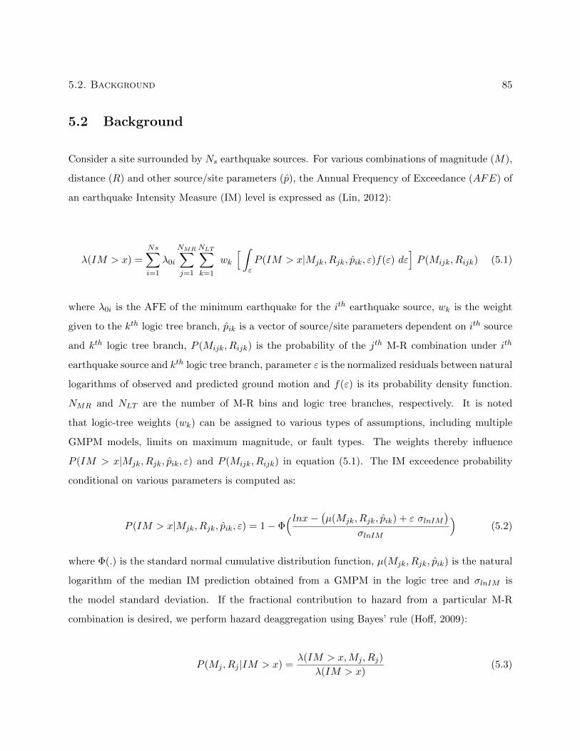
5.2. Background 85
5.2 Background
Consider a site surrounded by Ns earthquake sources. For various combinations of magnitude (M),
distance (R) and other source/site parameters (p), the Annual Frequency of Exceedance (AFE) of
an earthquake Intensity Measure (IM) level is expressed as (Lin, 2012):
λ(IM > x) =Ns∑i=1
λ0i
NMR∑j=1
NLT∑k=1
wk
[ ∫εP (IM > x|Mjk, Rjk, pik, ε)f(ε) dε
]P (Mijk, Rijk) (5.1)
where λ0i is the AFE of the minimum earthquake for the ith earthquake source, wk is the weight
given to the kth logic tree branch, pik is a vector of source/site parameters dependent on ith source
and kth logic tree branch, P (Mijk, Rijk) is the probability of the jth M-R combination under ith
earthquake source and kth logic tree branch, parameter ε is the normalized residuals between natural
logarithms of observed and predicted ground motion and f(ε) is its probability density function.
NMR and NLT are the number of M-R bins and logic tree branches, respectively. It is noted
that logic-tree weights (wk) can be assigned to various types of assumptions, including multiple
GMPM models, limits on maximum magnitude, or fault types. The weights thereby influence
P (IM > x|Mjk, Rjk, pik, ε) and P (Mijk, Rijk) in equation (5.1). The IM exceedence probability
conditional on various parameters is computed as:
P (IM > x|Mjk, Rjk, pik, ε) = 1− Φ( lnx− (µ(Mjk, Rjk, pik) + ε σlnIM
)σlnIM
)(5.2)
where Φ(.) is the standard normal cumulative distribution function, µ(Mjk, Rjk, pik) is the natural
logarithm of the median IM prediction obtained from a GMPM in the logic tree and σlnIM is
the model standard deviation. If the fractional contribution to hazard from a particular M-R
combination is desired, we perform hazard deaggregation using Bayes’ rule (Hoff, 2009):
P (Mj , Rj |IM > x) =λ(IM > x,Mj , Rj)
λ(IM > x)(5.3)

86Chapter 5. A pre-configured solution to the problem of joint hazard estimation
given a suite of seismic intensity measures
where λ(IM > x,Mj , Rj) is the rate of earthquakes with IM > x, M = Mj and R = Rj . It
is noted that the numerator in the above equation is a subset of the sample space with specific
values of M-R, while the denominator is the entire sample space. λ(IM > x,Mj , Rj) can be further
expressed as:
λ(IM > x,Mj , Rj) =Ns∑i=1
λ0i
NLT∑k=1
wk P (IM > x|Mjk, Rjk, pik) P (Mijk, Rijk) (5.4)
where P (IM > x|Mjk, Rjk, pik) is obtained by integrating over all possible values of ε represented
by terms in the square bracket in equation (5.1).
Example seismic hazard analysis for a hypothetical site
A hypothetical site (located at the origin (0, 0)) surrounded by two faults modeled as line sources
will be used to perform a scalar seismic hazard analysis, and also to demonstrate the vector hazard
and deaggregation procedure proposed in this chapter. A truncated Gutenberg-Richter model is
used to construct a probability distribution for magnitudes, and a simple point model is adopted
to account for the uncertainty in hypocenter location. Point models consider the uncertainty only
in the rupture initiation point without regard to the uncertainty in rupture length (Kramer, 1996).
Epsilons are not truncated for the seismic hazard computations at this site. The average shear
wave velocity over the top thirty meters (V s30) is assumed to be 400 m/s. Other fault parameters
that will be relevant for modeling purposes are provided in Table 5.1.
A logic-tree is used for this hypothetical site to capture the epistemic uncertainty associated
with establishing maximum magnitudes, GMPM selection, and fault type. The logic-tree comprises
eight final branches, with two options each for: maximum magnitude (Mmax = 7 or 7.5), GMPM
(either Campbell and Bozorgnia 2008 or Boore and Atkinson 2008), and fault-type (either Reverse
or Normal faulting mechanism). A depiction of this logic-tree is provided in Figure 5.1 along with
the weights given to each of its branches.
Figure 5.2a provides the seismic hazard curves for the IM Sa(2s) computed under the standard
PSHA using a logic-tree approach; both the individual logic-tree branches and the final weighted
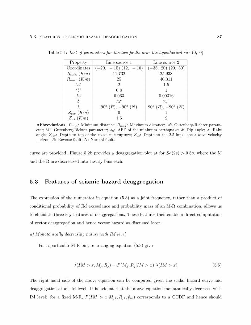
5.3. Features of seismic hazard deaggregation 87
Table 5.1: List of parameters for the two faults near the hypothetical site (0, 0)
Property Line source 1 Line source 2
Coordinates (−20, − 15) (12, − 10) (−35, 20) (20, 30)Rmin (Km) 11.732 25.938Rmax (Km) 25 40.311
‘a’ 2 1.5‘b’ 0.8 1λ0 0.063 0.00316δ 75o 75o
λ 90o (R), −90o (N) 90o (R), −90o (N)Ztor (Km) 0 1Zvs (Km) 1.5 2
Abbreviations. Rmin: Minimum distance; Rmax: Maximum distance; ‘a’: Gutenberg-Richter param-eter; ‘b’: Gutenberg-Richter parameter; λ0: AFE of the minimum earthquake; δ: Dip angle; λ: Rakeangle; Ztor: Depth to top of the co-seismic rupture; Zvs: Depth to the 2.5 km/s shear-wave velocityhorizon; R: Reverse fault; N : Normal fault.
curve are provided. Figure 5.2b provides a deaggregation plot at for Sa(2s) > 0.5g, where the M
and the R are discretized into twenty bins each.
5.3 Features of seismic hazard deaggregation
The expression of the numerator in equation (5.3) as a joint frequency, rather than a product of
conditional probability of IM exceedance and probability mass of an M-R combination, allows us
to elucidate three key features of deaggregations. These features then enable a direct computation
of vector deaggregation and hence vector hazard as discussed later.
a) Monotonically decreasing nature with IM level
For a particular M-R bin, re-arranging equation (5.3) gives:
λ(IM > x,Mj , Rj) = P (Mj , Rj |IM > x) λ(IM > x) (5.5)
The right hand side of the above equation can be computed given the scalar hazard curve and
deaggregation at an IM level. It is evident that the above equation monotonically decreases with
IM level: for a fixed M-R, P (IM > x|Mjk, Rjk, pik) corresponds to a CCDF and hence should

88Chapter 5. A pre-configured solution to the problem of joint hazard estimation
given a suite of seismic intensity measures
Mmax = 7.5
GMPM : BA
Fault Type : N0.7
Fault Type : R0.3
0.5
GMPM : CB0.5
0.6
Mmax = 7
0.4
Figure 5.1: Depiction of the logic-tree used for the hypothetical site considered in this study. Onlyunique branches arising at each rightward step are represented (there are eight final branches).A fraction along each of the branch arrows represents the weight given to that rightward step.Abbreviations: Campbell-Bozorgnia 2008 (CB), Boore-Atkinson 2008 (BA), Reverse fault (R),Normal fault (N).
decrease as the IM level increases, thus λ(IM > x,Mj , Rj) should also decrease as the IM level
increases (see equation 5.4). Figure 5.3 provides examples of the λ(IM > x,Mj , Rj) function
(equation 5.5) with IM level for the two M-R combinations at the hypothetical site.
The monotonically decreasing nature of deaggregation matrices highlights the fact that these
matrices are also a function of IM level. This will enable us to derive a quantity, termed the
aggregate conditional probability of IM exceedence, later on that eases the computation of vector
hazard/deaggregation.
b) Invariance to any minimum IM level
A second interesting property of deaggregations is their invariance to the choice of IM for a
low IM level. If in equation (5.4), the IM level selected is sufficiently low, P (IM > x|Mjk, Rjk, pik)
would be unity for all M-R combinations: i.e., all earthquakes must cause at least some ground
motion. Then equations (5.4) or (5.5) would simply represent the distribution of M-R and hence
be invariant to any choice of IM. This is mathematically expressed as:
λ(IM1 > xmin,Mj , Rj) = λ(IM2 > ymin,Mj , Rj) = λ(Mj , Rj) (5.6)
where xmin and ymin are minimum levels for the IMs IM1 and IM2 respectively. Figure 5.4 provides,
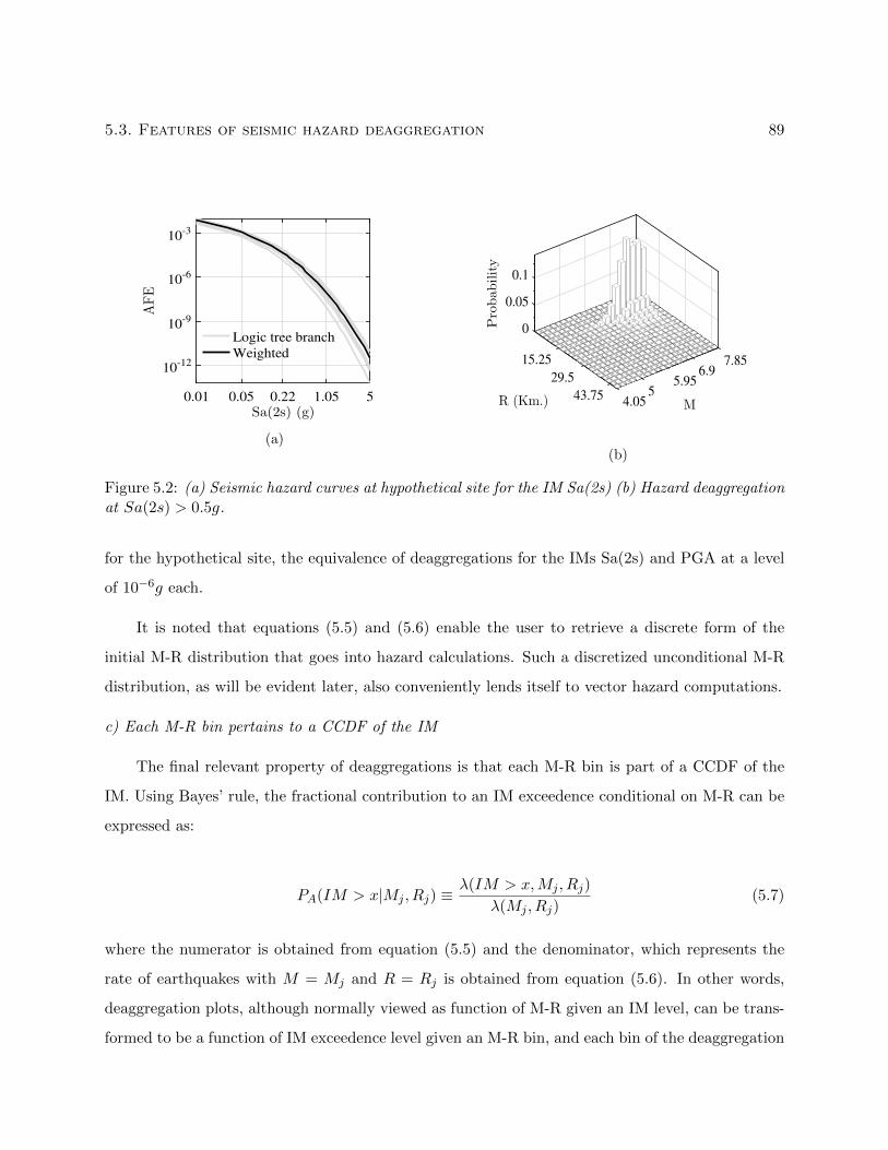
5.3. Features of seismic hazard deaggregation 89
0.01 0.05 0.22 1.05 5Sa(2s) (g)
10-12
10-9
10-6
10-3
AFE
Logic tree branch
Weighted
(a)
0
0.05
Probability
0.1
15.25 7.85
R (Km.)
6.9
M
29.5 5.955 43.75
4.05
(b)
Figure 5.2: (a) Seismic hazard curves at hypothetical site for the IM Sa(2s) (b) Hazard deaggregationat Sa(2s) > 0.5g.
for the hypothetical site, the equivalence of deaggregations for the IMs Sa(2s) and PGA at a level
of 10−6g each.
It is noted that equations (5.5) and (5.6) enable the user to retrieve a discrete form of the
initial M-R distribution that goes into hazard calculations. Such a discretized unconditional M-R
distribution, as will be evident later, also conveniently lends itself to vector hazard computations.
c) Each M-R bin pertains to a CCDF of the IM
The final relevant property of deaggregations is that each M-R bin is part of a CCDF of the
IM. Using Bayes’ rule, the fractional contribution to an IM exceedence conditional on M-R can be
expressed as:
PA(IM > x|Mj , Rj) ≡λ(IM > x,Mj , Rj)
λ(Mj , Rj)(5.7)
where the numerator is obtained from equation (5.5) and the denominator, which represents the
rate of earthquakes with M = Mj and R = Rj is obtained from equation (5.6). In other words,
deaggregation plots, although normally viewed as function of M-R given an IM level, can be trans-
formed to be a function of IM exceedence level given an M-R bin, and each bin of the deaggregation
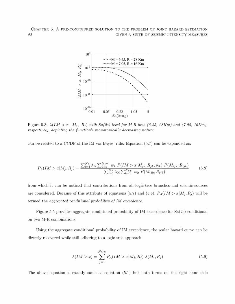
90Chapter 5. A pre-configured solution to the problem of joint hazard estimation
given a suite of seismic intensity measures
0.01 0.05 0.22 1.05 5
Sa(2s)(g)
10-20
10-15
10-10
10-5
100
λ(IM
>x,M
j,R
j)
M = 6.45, R = 28 Km
M = 7.05, R = 16 Km
Figure 5.3: λ(IM > x, Mj , Rj) with Sa(2s) level for M-R bins (6.45, 28Km) and (7.05, 16Km),respectively, depicting the function’s monotonically decreasing nature.
can be related to a CCDF of the IM via Bayes’ rule. Equation (5.7) can be expanded as:
PA(IM > x|Mj , Rj) =
∑Nsi=1 λ0i
∑NLTk=1 wk P (IM > x|Mjk, Rjk, pik) P (Mijk, Rijk)∑Ns
i=1 λ0i∑NLT
k=1 wk P (Mijk, Rijk)(5.8)
from which it can be noticed that contributions from all logic-tree branches and seismic sources
are considered. Because of this attribute of equations (5.7) and (5.8), PA(IM > x|Mj , Rj) will be
termed the aggregated conditional probability of IM exceedence.
Figure 5.5 provides aggregate conditional probability of IM exceedence for Sa(2s) conditional
on two M-R combinations.
Using the aggregate conditional probability of IM exceedence, the scalar hazard curve can be
directly recovered while still adhering to a logic tree approach:
λ(IM > x) =
NMR∑j=1
PA(IM > x|Mj , Rj) λ(Mj , Rj) (5.9)
The above equation is exactly same as equation (5.1) but both terms on the right hand side

5.3. Features of seismic hazard deaggregation 91
0
0.005
λ(S
a(2s)
>1e
−6,M
j,R
j)
15.25 7.85
R (Km.)
6.9
M
29.5 5.955 43.75
4.05
(a) Sa(2s)
0
0.005
λ(P
GA
>1e
−6,M
j,R
j)
15.25 7.85
R (Km.)
6.9
M
29.5 5.955 43.75
4.05
(b) PGA
Figure 5.4: Invariance of deaggregations with the choice of IM for a low IM level (1e-6 g)
are obtained directly from deaggregation. This equivalence will be evident when the aggregate
conditional probability of IM exceedence is expanded by substituting the definition of PA(IM >
x|Mj , Rj) (equation 5.8) into equation (5.9):
λ(IM > x) =
NMR∑j=1
∑Nsi=1 λ0i
∑NLTk=1 wk P (IM > x|Mjk, Rjk, pik) P (Mijk, Rijk)
λ(Mj , Rj)λ(Mj , Rj) (5.10)
which is same as equation (5.1) except that the integration with the parameter ε has been sup-
pressed for brevity and the order of summation has been interchanged. The aggregate conditional
probability of IM exceedence, although having a similar mathematical notation, is not equal to the
conditional probability of IM level exceedence directly obtained from a GMPM. The equivalence
of these quantities only holds true when a single GMPM is used in the logic tree and this GMPM
does not consider earthquake source related parameters. This is mathematically expressed as:
PA(IM > x|Mj , Rj) =P (IM > x|Mj , Rj , p)
∑Nsi=1 λ0i
∑NLTk=1 wk P (Mijk, Rijk)∑Ns
i=1 λ0i∑NLT
k=1 wk P (Mijk, Rijk)(5.11)
where P (IM > x|Mj , Rj , p) in the numerator shows that a single GMPM which is independent
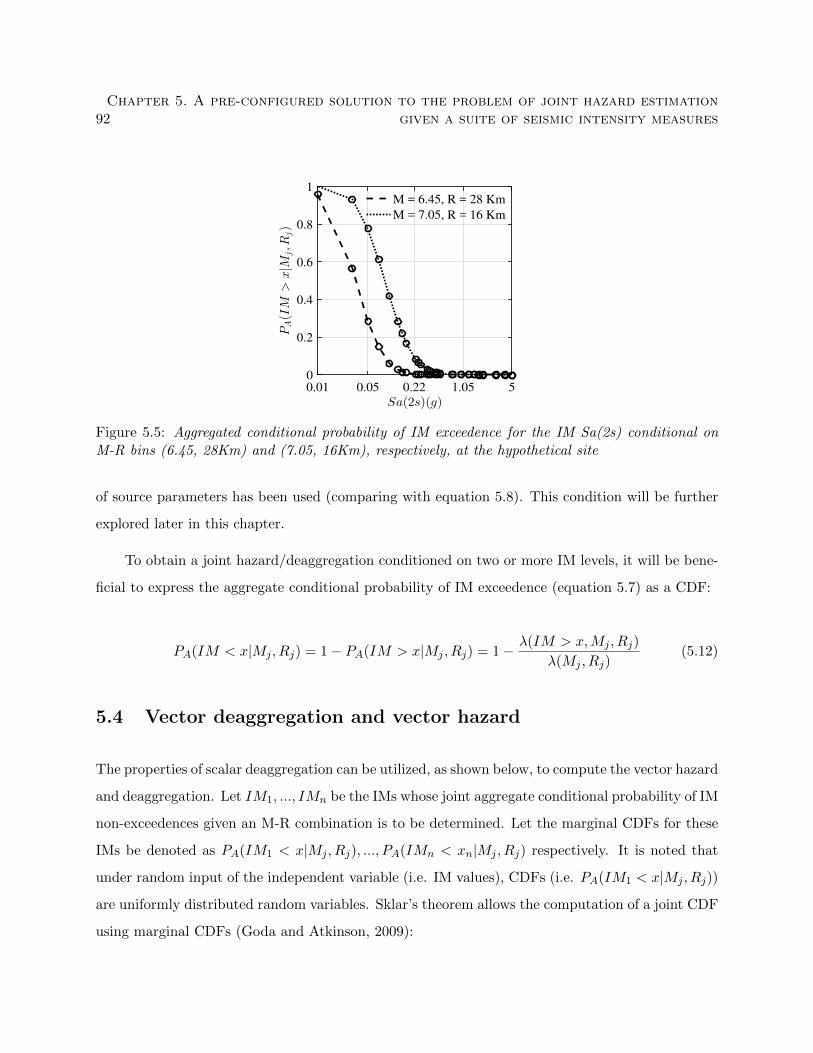
92Chapter 5. A pre-configured solution to the problem of joint hazard estimation
given a suite of seismic intensity measures
0.01 0.05 0.22 1.05 5
Sa(2s)(g)
0
0.2
0.4
0.6
0.8
1
PA(IM
>x|M
j,R
j)
M = 6.45, R = 28 Km
M = 7.05, R = 16 Km
Figure 5.5: Aggregated conditional probability of IM exceedence for the IM Sa(2s) conditional onM-R bins (6.45, 28Km) and (7.05, 16Km), respectively, at the hypothetical site
of source parameters has been used (comparing with equation 5.8). This condition will be further
explored later in this chapter.
To obtain a joint hazard/deaggregation conditioned on two or more IM levels, it will be bene-
ficial to express the aggregate conditional probability of IM exceedence (equation 5.7) as a CDF:
PA(IM < x|Mj , Rj) = 1− PA(IM > x|Mj , Rj) = 1− λ(IM > x,Mj , Rj)
λ(Mj , Rj)(5.12)
5.4 Vector deaggregation and vector hazard
The properties of scalar deaggregation can be utilized, as shown below, to compute the vector hazard
and deaggregation. Let IM1, ..., IMn be the IMs whose joint aggregate conditional probability of IM
non-exceedences given an M-R combination is to be determined. Let the marginal CDFs for these
IMs be denoted as PA(IM1 < x|Mj , Rj), ..., PA(IMn < xn|Mj , Rj) respectively. It is noted that
under random input of the independent variable (i.e. IM values), CDFs (i.e. PA(IM1 < x|Mj , Rj))
are uniformly distributed random variables. Sklar’s theorem allows the computation of a joint CDF
using marginal CDFs (Goda and Atkinson, 2009):
5.4. Vector deaggregation and vector hazard 93
PA(IM1 < x1, ..., IMn < xn|Mj , Rj)
= C(PA(IM1 < x|Mj , Rj), ..., PA(IMn < xn|Mj , Rj)
)= C(u1, ..., un)
(5.13)
where C is a Copula function and u denotes a uniformly distributed random variable. A Copula
function attempts to capture nonlinear (or non-Gaussian) dependences between random variables
through their marginal CDFs. As a result of its aggregation across logic-tree branches and multiple
fault sources, the aggregated conditional probability of an IM non-exceedence is likely to be a non-
Gaussian marginal. Hence the goal is to compute the non-Gaussian distributed joint aggregated
conditional probability of a vector IM non-exceedences through a Copula function and then to use
the properties of scalar deaggregations to find the vector hazard/deaggregation.
Despite its name, a Gaussian Copula is frequently preferred to capture nonlinear depen-
dences between random variables owing to its ease-of-use and its acceptable performance (Goda
and Atkinson, 2009). This Copula is termed ‘Gaussian’ due to its reliance on Pearson corre-
lation coefficients to relate the marginal CDFs of two or more random variables arising from
arbitrary probability density distributions and its ability to recover a bivariate Gaussian if the
marginals of two random variables are Gaussian. Given the correlation matrix between various
IMs and uniformly distributed random variables (u1, ..., un, which represent the aggregated CDFs
PA(IM1 < x|Mj , Rj), ..., PA(IMn < xn|Mj , Rj) respectively), a Gaussian copula is defined as:
C(u1, ..., un) = Φ(Φ−1(u1), ...,Φ
−1(un))
(5.14)
where Φ−1 denotes a scalar inverse standard Gaussian CDF and Φ is a multivariate Gaussian
CDF with a zero mean vector and a covariance matrix equal to the correlation matrix between the
IMs. Thus all that is necessary to obtain the vector hazard is the correlation matrix of the IMs.
In this work, it is assumed that the same correlation matrix between the IMs holds for various
M-R combinations—an assumption supported by Baker and Bradley (2017) who conclude that
correlations between various IMs show no significant dependence on M-R and site characteristics
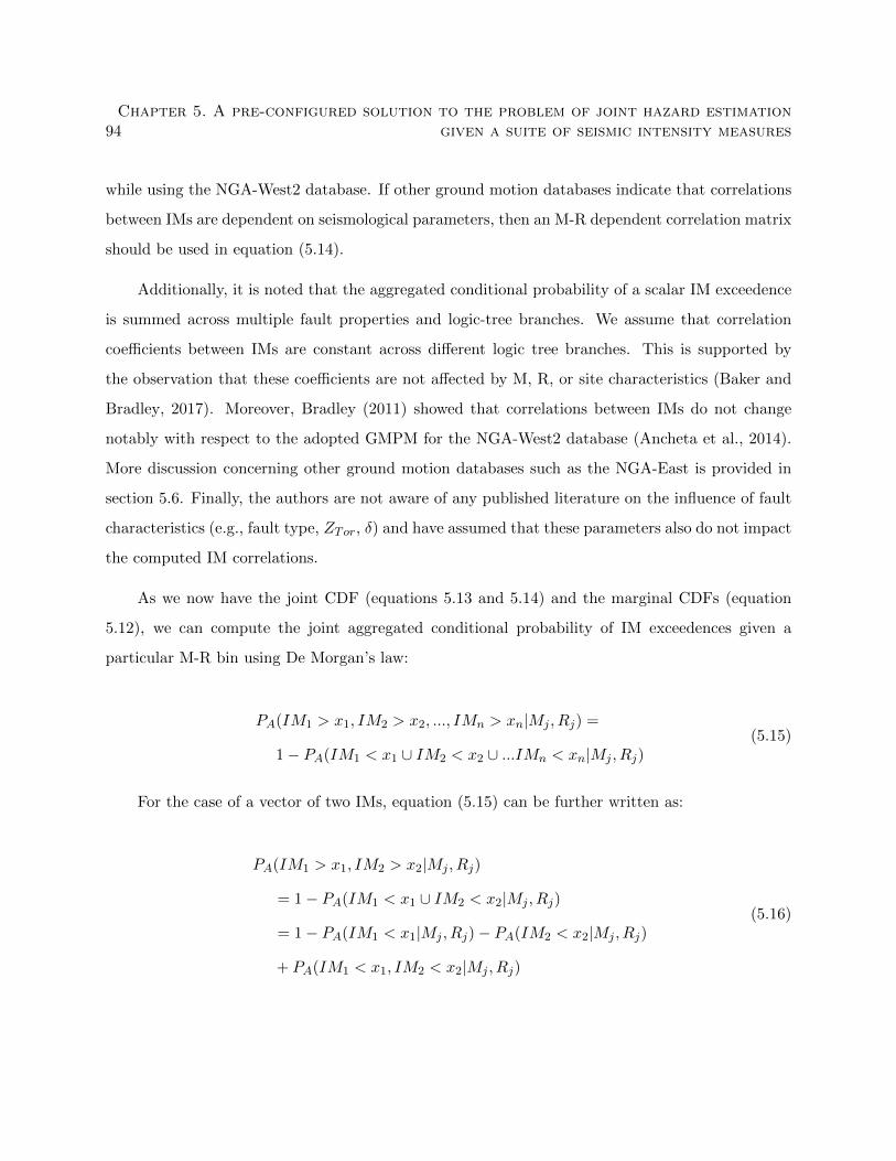
94Chapter 5. A pre-configured solution to the problem of joint hazard estimation
given a suite of seismic intensity measures
while using the NGA-West2 database. If other ground motion databases indicate that correlations
between IMs are dependent on seismological parameters, then an M-R dependent correlation matrix
should be used in equation (5.14).
Additionally, it is noted that the aggregated conditional probability of a scalar IM exceedence
is summed across multiple fault properties and logic-tree branches. We assume that correlation
coefficients between IMs are constant across different logic tree branches. This is supported by
the observation that these coefficients are not affected by M, R, or site characteristics (Baker and
Bradley, 2017). Moreover, Bradley (2011) showed that correlations between IMs do not change
notably with respect to the adopted GMPM for the NGA-West2 database (Ancheta et al., 2014).
More discussion concerning other ground motion databases such as the NGA-East is provided in
section 5.6. Finally, the authors are not aware of any published literature on the influence of fault
characteristics (e.g., fault type, ZTor, δ) and have assumed that these parameters also do not impact
the computed IM correlations.
As we now have the joint CDF (equations 5.13 and 5.14) and the marginal CDFs (equation
5.12), we can compute the joint aggregated conditional probability of IM exceedences given a
particular M-R bin using De Morgan’s law:
PA(IM1 > x1, IM2 > x2, ..., IMn > xn|Mj , Rj) =
1− PA(IM1 < x1 ∪ IM2 < x2 ∪ ...IMn < xn|Mj , Rj)(5.15)
For the case of a vector of two IMs, equation (5.15) can be further written as:
PA(IM1 > x1, IM2 > x2|Mj , Rj)
= 1− PA(IM1 < x1 ∪ IM2 < x2|Mj , Rj)
= 1− PA(IM1 < x1|Mj , Rj)− PA(IM2 < x2|Mj , Rj)
+ PA(IM1 < x1, IM2 < x2|Mj , Rj)
(5.16)
5.4. Vector deaggregation and vector hazard 95
5.4.1 Manipulations to compute the vector hazard/deaggregation
The joint aggregated conditional probability of IM exceedence can be expanded as:
PA(IM1 > x1, ..., IMn > xn|Mj , Rj) =∑Nsi=1 λ0i
∑NLTk=1 wk P (IM1 > x1, ..., IMn > xn|Mjk, Rjk, pik) P (Mijk, Rijk)∑Ns
i=1 λ0i∑NLT
k=1 wk P (Mijk, Rijk)
(5.17)
Then, invoking the invariance property of deaggregations, the joint rate is computed by modifying
equation (5.7) to the vector IM case as shown below:
λ(IM1 > x1, ..., IMn > xn,Mj , Rj) = PA(IM1 > x1, ..., IMn > xn|Mj , Rj) λ(Mj , Rj) (5.18)
the vector seismic hazard (which is a normalizing constant in the Bayes’ rule application) is com-
puted by summing equation (5.18) across all M-R bins:
λ(IM1 > x1, ..., IMn > xn)
=
NMR∑j=1
λ(IM1 > x1, ..., IMn > xn,Mj , Rj)
=
NMR∑j=1
∑Nsi=1 λ0i
∑NMk=1 wk P (IM1 > x1, ..., IMn > xn|Mjk, Rjk, pik) P (Mijk, Rijk)
λ(Mj , Rj)λ(Mj , Rj)
(5.19)
which follows the definition of vector seismic hazard while respecting the fault-specific parameters
for the multiple seismic sources. The above equation is also seen to consider the multiple branches
of a logic tree. Now, the vector deaggregation can be found by dividing equation (5.18) by its
normalizing constant (equation 5.19):
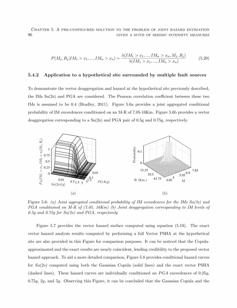
96Chapter 5. A pre-configured solution to the problem of joint hazard estimation
given a suite of seismic intensity measures
P (Mj , Rj |IM1 > x1, ..., IMn > xn) =λ(IM1 > x1, ..., IMn > xn,Mj , Rj)
λ(IM1 > x1, ..., IMn > xn)(5.20)
5.4.2 Application to a hypothetical site surrounded by multiple fault sources
To demonstrate the vector deaggregation and hazard at the hypothetical site previously described,
the IMs Sa(2s) and PGA are considered. The Pearson correlation coefficient between these two
IMs is assumed to be 0.4 (Bradley, 2011). Figure 5.6a provides a joint aggregated conditional
probability of IM exceedences conditioned on an M-R of 7.05-16Km. Figure 5.6b provides a vector
deaggregation corresponding to a Sa(2s) and PGA pair of 0.5g and 0.75g, respectively.
0.01
PGA(g)
0
0.3
0.25
Sa(2s)(g)
0.01 1.5
0.5
0.3
PA(IM
1>
x1,IM
2>
x2|M
j,R
j)
51.5 5
0.75
1
(a)
0
0.1
Probab
ility
15.25 7.85
R (Km.)
6.9
M
29.5 5.955 43.75
4.05
(b)
Figure 5.6: (a) Joint aggregated conditional probability of IM exceedences for the IMs Sa(2s) andPGA conditioned on M-R of (7.05, 16Km) (b) Joint deaggregation corresponding to IM levels of0.5g and 0.75g for Sa(2s) and PGA, respectively
Figure 5.7 provides the vector hazard surface computed using equation (5.19). The exact
vector hazard analysis results computed by performing a full Vector PSHA at the hypothetical
site are also provided in this Figure for comparison purposes. It can be noticed that the Copula-
approximated and the exact results are nearly coincident, lending credibility to the proposed vector
hazard approach. To aid a more detailed comparison, Figure 5.8 provides conditional hazard curves
for Sa(2s) computed using both the Gaussian Copula (solid lines) and the exact vector PSHA
(dashed lines). These hazard curves are individually conditioned on PGA exceedences of 0.25g,
0.75g, 2g, and 5g. Observing this Figure, it can be concluded that the Gaussian Copula and the
5.4. Vector deaggregation and vector hazard 97
exact results compare very well. Any slight discrepancies, especially at IM levels of (Sa(2s) >
5g, PGA > 5g), can be attributed to inaccuracies in Gaussian Copula approximation of the joint
aggregated conditional probability of IM exceedences. Other Copula types, say a ‘t’ or a Clayton
Copula, can be explored in their capability to more accurately capture the PA(IM1 > x1, ..., IMn >
xn|Mj , Rj) and the performance of different Copula types can be compared. However, such an
investigation is outside of the scope of this dissertation and will be treated in a future study;
however, an interested reader may refer to appendix B for a preliminary investigation on the choice
of Copulas.
10-15
10-12
PGA(g)
10-9
0.25
λ(S
a(2s)>
x1,PGA
>x2)
10-6
Sa(2s)(g)
0.25
10-3
11
55
Gaussian Copula
Exact
Figure 5.7: Vector hazard surface for the IMs Sa(2s) and PGA computed using a Gaussian Copula.The exact vector hazard analysis results are also provided for comparison purposes.
Because the joint AFE can be as low as 10−15 at this hypothetical site, use of proper numerical
accuracy for computations becomes important. We used double precision numerical accuracy for
all our calculations including the exact vector PSHA. In addition, we note that the accuracy of our
method for simplified Vector PSHA may depend upon the bin size of deaggregation plots with finer
discretizations potentially leading to more accurate estimation of the joint hazard.
A sequence of steps required to compute vector deaggregation and vector hazard given the
scalar deaggregations for the various IMs under consideration is shown in algorithm 3.

98Chapter 5. A pre-configured solution to the problem of joint hazard estimation
given a suite of seismic intensity measures
0.01 0.25 1 5Sa(2s)(g)
10-15
10-10
10-5
100
λ(S
a(2s)>
x1,P
GA
>x2)
Lines: Gaussian Copula, Circles: Exact
PGA > 0.25g
PGA > 0.75g
PGA > 2g
PGA > 5g
Figure 5.8: Conditional hazard curves for Sa(2s) computed using both Gaussian Copula (solidlines) and exact vector hazard analysis (circles). These hazard curves are conditioned on PGAexceedences of 0.25g, 0.75g, 2g, and 5g.
5.5 Application of the proposed vector hazard approach to a real
site in Los Angeles, CA
We apply the proposed vector hazard analysis approach to a real site in Los Angeles, CA [33.996oN ; 118.162oW ].
The same two IMs, Sa(2s) and PGA, are used for vector hazard computations. OpenSHA soft-
ware (Field et al., 2003) was used to obtain the scalar hazard curves and the deaggregations at
several IM levels using the 2008 Boore and Atkinson GMPM and assuming a Vs30 of 300 m/s.
The USGS/CGS 1996 Adj. Cal. Earthquake Rupture Forecast was used for PSHA computations.
The deaggregation matrices were discretized to have twenty-four magnitude bins and twenty-three
distance bins.
Upon retrieving the scalar hazard curves and deaggregation matrices for the two IMs and
their intensities of interest from OpenSHA, the following computations (numbered according to the
related step in Algorithm 5.1) are implemented to compute vector hazard and deaggregation:
2: Given an IM level and an M-R bin in the deaggregation matrix, the joint frequency (λ(IM >
x,Mj , Rj)) is found by multiplying the probability mass of this M-R bin with the seismic
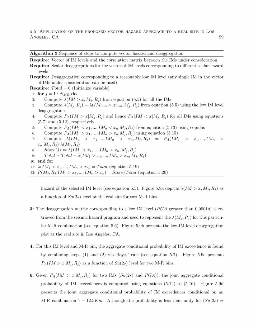
5.5. Application of the proposed vector hazard approach to a real site in LosAngeles, CA 99
Algorithm 3 Sequence of steps to compute vector hazard and deaggregation
Require: Vector of IM levels and the correlation matrix between the IMs under considerationRequire: Scalar deaggregations for the vector of IM levels corresponding to different scalar hazard
levelsRequire: Deaggregation corresponding to a reasonably low IM level (any single IM in the vector
of IMs under consideration can be used)Require: Total = 0 (Initialize variable)
1: for j = 1 : NMR do2: Compute λ(IM > x,Mj , Rj) from equation (5.5) for all the IMs3: Compute λ(Mj , Rj) = λ(IMmin > xmin,Mj , Rj) from equation (5.5) using the low IM level
deaggregation4: Compute PA(IM > x|Mj , Rj) and hence PA(IM < x|Mj , Rj) for all IMs using equations
(5.7) and (5.12), respectively5: Compute PA(IM1 < x1, ..., IMn < xn|Mj , Rj) from equation (5.13) using copulas6: Compute PA(IM1 > x1, ..., IMn > xn|Mj , Rj) using equation (5.15)7: Compute λ(IM1 > x1, ..., IMn > xn,Mj , Rj) = PA(IM1 > x1, ..., IMn >xn|Mj , Rj) λ(Mj , Rj)
8: Store(j)⇐ λ(IM1 > x1, ..., IMn > xn,Mj , Rj)9: Total = Total + λ(IM1 > x1, ..., IMn > xn,Mj , Rj)
10: end for11: λ(IM1 > x1, ..., IMn > xn) = Total (equation 5.19)12: P (Mj , Rj |IM1 > x1, ..., IMn > xn) = Store/Total (equation 5.20)
hazard of the selected IM level (see equation 5.5). Figure 5.9a depicts λ(IM > x,Mj , Rj) as
a function of Sa(2s) level at the real site for two M-R bins.
3: The deaggregation matrix corresponding to a low IM level (PGA greater than 0.0001g) is re-
trieved from the seismic hazard program and used to represent the λ(Mj , Rj) for this particu-
lar M-R combination (see equation 5.6). Figure 5.9b presents the low-IM-level deaggregation
plot at the real site in Los Angeles, CA.
4: For this IM level and M-R bin, the aggregate conditional probability of IM exceedence is found
by combining steps (1) and (2) via Bayes’ rule (see equation 5.7). Figure 5.9c presents
PA(IM > x|Mj , Rj) as a function of Sa(2s) level for two M-R bins.
6: Given PA(IM > x|Mj , Rj) for two IMs (Sa(2s) and PGA)), the joint aggregate conditional
probability of IM exceedences is computed using equations (5.12) to (5.16). Figure 5.9d
presents the joint aggregate conditional probability of IM exceedences conditional on an
M-R combination 7 − 12.5Km. Although the probability is less than unity for (Sa(2s) =
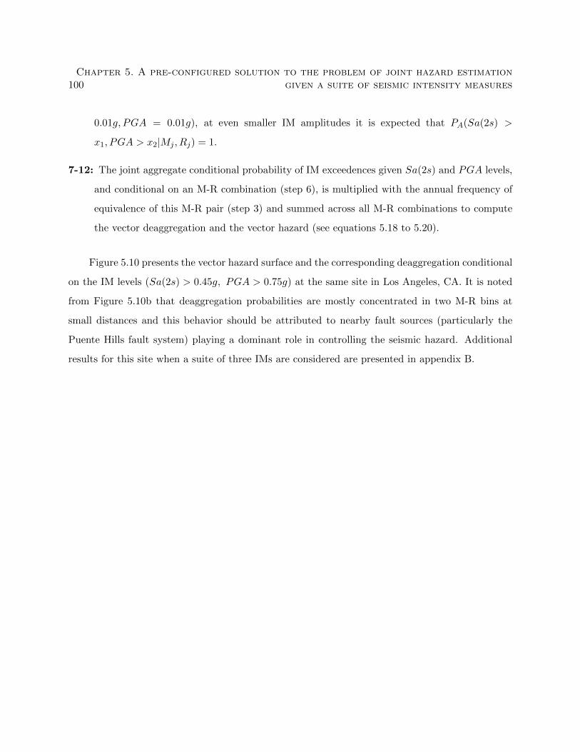
100Chapter 5. A pre-configured solution to the problem of joint hazard estimation
given a suite of seismic intensity measures
0.01g, PGA = 0.01g), at even smaller IM amplitudes it is expected that PA(Sa(2s) >
x1, PGA > x2|Mj , Rj) = 1.
7-12: The joint aggregate conditional probability of IM exceedences given Sa(2s) and PGA levels,
and conditional on an M-R combination (step 6), is multiplied with the annual frequency of
equivalence of this M-R pair (step 3) and summed across all M-R combinations to compute
the vector deaggregation and the vector hazard (see equations 5.18 to 5.20).
Figure 5.10 presents the vector hazard surface and the corresponding deaggregation conditional
on the IM levels (Sa(2s) > 0.45g, PGA > 0.75g) at the same site in Los Angeles, CA. It is noted
from Figure 5.10b that deaggregation probabilities are mostly concentrated in two M-R bins at
small distances and this behavior should be attributed to nearby fault sources (particularly the
Puente Hills fault system) playing a dominant role in controlling the seismic hazard. Additional
results for this site when a suite of three IMs are considered are presented in appendix B.
5.6. Discussion of Intensity Measure correlation coefficients in relation to theproposed vector hazard approach 101
0.01 0.1 1 4
Sa(2s)(g)
10-11
10-9
10-7
10-5
10-3
λ(IM
>x,M
j,R
j)
M = 6.5, R = 27.5 Km
M = 7, R = 12.5 Km
(a)
0
0.01
4
λ(S
a(2s)
>0.0001g,M
j,R
j)
1205100
M
6 80
R (Km.)
60 740 8 20
0
(b)
n
0.01 0.1 1 4
Sa(2s)(g)
0
0.2
0.4
0.6
0.8
1
PA(IM
>x|M
j,R
j)
M = 6.5, R = 27.5 Km
M = 7, R = 12.5 Km
(c)
0.01
0.25
0.25
PGA(g)
0.5
Sa(2s)(g)
0.25
PA(IM
1>
x1,IM
2>
x2|M
j,R
j)
1
0.75
14
1
4
(d)
Figure 5.9: (a) Depiction of λ(IM > x,Mj , Rj) as a function of Sa(2s) level at the real site in LosAngeles, CA for two M-R bins; (b) Low-IM-level deaggregation plot at this site (PGA greater than0.0001g); (c) Aggregate conditional probability of IM exceedence as function of Sa(2s) level for twoM-R bins at this site; (d) Joint aggregate conditional probability of IM exceedences for the two IMsSa(2s) and PGA, and conditional on a M-R combination 7− 12.5Km.
5.6 Discussion of Intensity Measure correlation coefficients in re-
lation to the proposed vector hazard approach
The quantity PA(IM > x|Mj , Rj) can include multiple GMPMs weighted through a logic-tree
(see Figure 5.1). The computation of PA(IM1 > x1, . . . , IMn > xn|Mj , Rj), however, utilizes
the IM correlation coefficients derived through a single GMPM. To explore the adequacy of this
102Chapter 5. A pre-configured solution to the problem of joint hazard estimation
given a suite of seismic intensity measures
10-9
10-7
10-5
λ(S
a(2s)
>x1,P
GA
>x2)
10-3
0.25
10-1
PGA(g)Sa(2s)(g)
0.25 1144
(a)
0
0.2
0.4
4
Probab
ility 0.6
1205100
M
6 80
R (Km.)
60 740 8 20
0
(b)
Figure 5.10: (a) Vector hazard surface and the (b) Corresponding deaggregation conditional on theIM levels (Sa(2s) > 0.45g, PGA > 0.75g) at the same site in Los Angeles, CA.
disparity between the GMPMs used in the logic-tree and the GMPM adopted for computing IM
correlations, two case studies are considered. The first study considers a subset of the NGA-West2
database2 (Ancheta et al., 2014), and two corresponding GMPMs BA2008 and CB2008. The second
study considers a subset of the NGA-East database3 (Goulet et al., 2014), and two corresponding
GMPMs, Atkinson and Boore 2006 (AB2006) and Shahjouei and Pezeshk 2016 (SP2016). For both
these case studies, the correlations between PGA and SA are first computed using a single GMPM.
Next, these correlations are computed using the two GMPMs by assigning weights to replicate the
logic-tree. Finally, the different correlation values will be compared to verify whether the GMPM
weighting introduces additional correlation between IMs.
IM correlations are computed by first determining the ε values. ε is defined as:
εIMi =ln IMi − µlnIMi
σlnIMi
(5.21)
where IMi is the ith IM recording from the database, µ is the predicted IM value using a
GMPM, and σ is the standard deviation of the GMPM prediction. When two GMPMs are utilized
by assigning weights (w(1) and w(2), respectively; for the present case, these values are set to 0.5
each), the mean prediction and the standard deviation are computed using:
2496 recordings for which the Zvs value is available.3320 recordings on rock sites were used.
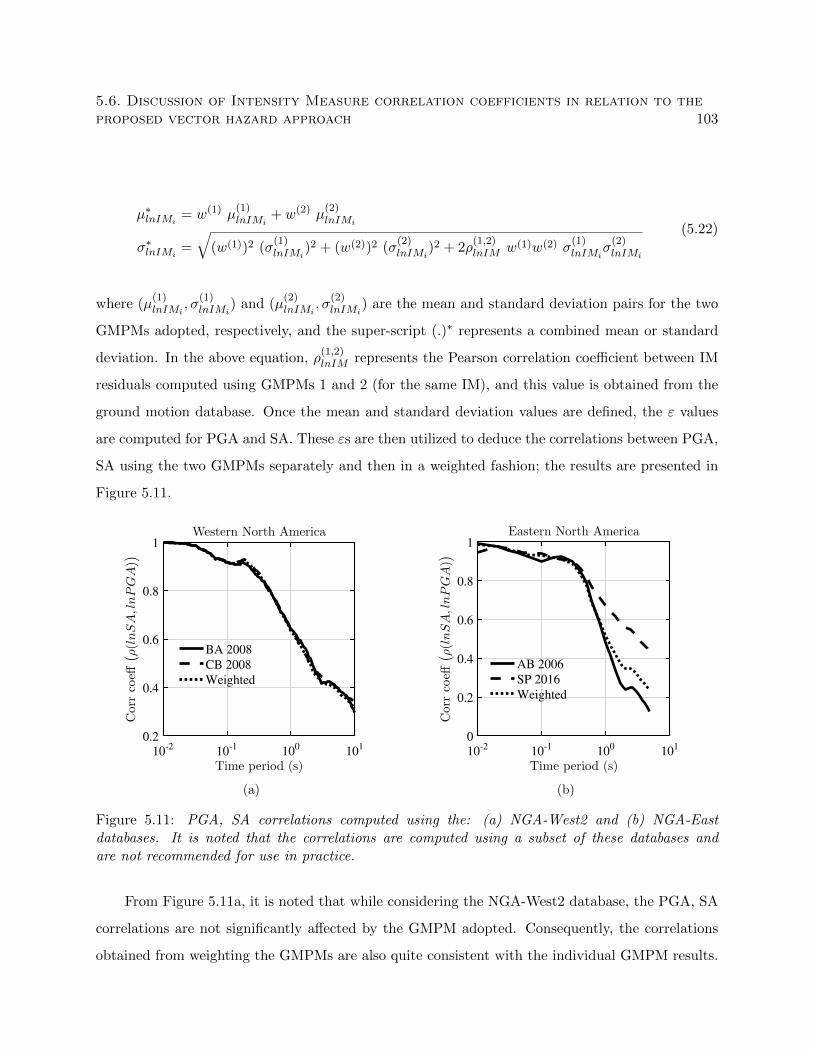
5.6. Discussion of Intensity Measure correlation coefficients in relation to theproposed vector hazard approach 103
µ∗lnIMi= w(1) µ
(1)lnIMi
+ w(2) µ(2)lnIMi
σ∗lnIMi=
√(w(1))2 (σ
(1)lnIMi
)2 + (w(2))2 (σ(2)lnIMi
)2 + 2ρ(1,2)lnIM w(1)w(2) σ
(1)lnIMi
σ(2)lnIMi
(5.22)
where (µ(1)lnIMi
, σ(1)lnIMi
) and (µ(2)lnIMi
, σ(2)lnIMi
) are the mean and standard deviation pairs for the two
GMPMs adopted, respectively, and the super-script (.)∗ represents a combined mean or standard
deviation. In the above equation, ρ(1,2)lnIM represents the Pearson correlation coefficient between IM
residuals computed using GMPMs 1 and 2 (for the same IM), and this value is obtained from the
ground motion database. Once the mean and standard deviation values are defined, the ε values
are computed for PGA and SA. These εs are then utilized to deduce the correlations between PGA,
SA using the two GMPMs separately and then in a weighted fashion; the results are presented in
Figure 5.11.
10-2 10-1 100 101
Time period (s)
0.2
0.4
0.6
0.8
1
Corr
coeff
(
ρ(lnSA,lnPGA))
Western North America
BA 2008
CB 2008
Weighted
(a)
10-2 10-1 100 101
Time period (s)
0
0.2
0.4
0.6
0.8
1
Corr
coeff
(
ρ(lnSA,lnPGA))
Eastern North America
AB 2006
SP 2016
Weighted
(b)
Figure 5.11: PGA, SA correlations computed using the: (a) NGA-West2 and (b) NGA-Eastdatabases. It is noted that the correlations are computed using a subset of these databases andare not recommended for use in practice.
From Figure 5.11a, it is noted that while considering the NGA-West2 database, the PGA, SA
correlations are not significantly affected by the GMPM adopted. Consequently, the correlations
obtained from weighting the GMPMs are also quite consistent with the individual GMPM results.
104Chapter 5. A pre-configured solution to the problem of joint hazard estimation
given a suite of seismic intensity measures
However, when considering the NGA-East database (Figure 5.11b), the correlations are influenced
by the GMPM adopted. This is because for the NGA-West2 database, mean predictions from
different GMPMs were observed to be close, whereas, for the NGA-East database, mean predictions
were not consistent across the GMPMs and therefore the correlations varied.
Inconsistencies in the predicted IM correlations across the different GMPMs in a logic-tree
can impact the vector hazard results. While a GMPM that produces lesser correlations than
weighted GMPMs leads to an underestimation of the vector hazard, a GMPM the produces greater
correlation than weighted GMPMs leads to an overestimation. This is because, the PA(IM1 >
x1, . . . , IMn > xn|Mj , Rj) is proportional to the IM correlations given a set of IMs, M, and R
values. In cases where it known that IM correlations across the GMPMs adopted are different, the
use of single-GMPM derived correlations are not recommended to be used in the proposed approach
for vector hazard analysis.
5.7 Can the invariance property be utilized to directly compute
scalar hazard curves using new a GMPM/IM?
With the addition of new earthquake records, ground motion databases around the world are
constantly expanding and GMPMs are frequently being updated (Boore and Atkinson 2008 to
Boore et al. 2014 for example). Moreover, many advanced IMs have been proposed that intend to
capture multiple aspects of ground motion and that have been shown to better predict structural
response than conventional IMs (such as Sa(T1); see Marafi et al. 2016 for example). Within the
framework of Performance Based Earthquake Engineering, these new GMPMs or IMs are only
useful if their seismic hazard curves are available, which would in general require re-programming
PSHA software to include these new GMPMs/IMs. If preliminary PSHA results could be obtained
with less effort it would support the rapid assessment of candidate IMs, e.g., evaluation of their
efficiency and sufficiency (Dhulipala et al., 2018b). This section therefore explores whether the
properties of scalar hazard deaggregations can be leveraged to estimate scalar hazard curves using
new GMPMs/IMs.
The invariance property of deaggregations is convenient in that it directly represents the
5.7. Can the invariance property be utilized to directly compute scalar hazardcurves using new a GMPM/IM? 105
relative importance of different M-R combinations without regard to the IM in terms of a fre-
quency (λ(Mj , Rj)). Given an M-R combination, the probability of exceedence of an IM level
(P (IM > x|Mj , Rj)) can be computed using the new GMPM or by fitting a GMPM to the new
IM. Then, the seismic hazard curve can directly be computed without performing a full PSHA for
the new IM using:
λ(IM > x) =
NMR∑j=1
P (IM > x|Mj , Rj) λ(Mj , Rj) (5.23)
which is exact only if P (IM > x|Mj , Rj) is equal to the aggregated conditional probability of IM
exceedence. As mentioned earlier in the discussion related to equation (5.11), P (IM > x|Mj , Rj)
and PA(IM > x|Mj , Rj) are equivalent only if a single GMPM is used in the logic tree and this
GMPM does not take into account source related parameters. Contemporary GMPMs, however,
require at least the type of the fault as an input, with more complicated GMPMs, such as CB2008,
requiring other parameters such as Ztor, Zvs, λ, and δ (refer to Table 5.1 for abbreviations).
The quality of the approximation made by equation (5.23) to compute the seismic hazard of
a scalar IM will be tested by assuming that the Boore and Atkinson (2008) with an unspecified
fault type is a new GMPM or a GMPM fitted to a new IM. Then, the computed hazard curve will
be compared with the one obtained from OpenSHA using the same GMPM but considering the
fault-specific characteristics. Figures 5.12a and 5.12b provide seismic hazard curves at the same
site in Los Angeles, CA for the IMs Sa(2s) and PGA from OpenSHA along with the approximate
hazard curves from equation (5.23). Given the low effort required in terms of not having to re-run
hazard calculations or having to re-program the PSHA software to include the new IM/GMPM, the
approximate hazard curve makes a reasonable prediction of the seismic hazard up to an IM level
0.5g for both Sa(2s) and PGA. After 0.5g, however, the the approximate curve starts to deviate
from the exact one and this effect is seen to be more prominent for PGA. So, the hazard curve
obtained from equation (5.23) can only be considered as a preliminary approximation and it needs
to be further tested for other sites and IMs. However, for a preliminary seismic risk assessment of
structures using advanced IMs or new GMPMs whose seismic hazard curves are unavailable from
PSHA programs, the approximate procedure for scalar hazard estimation proposed in this section
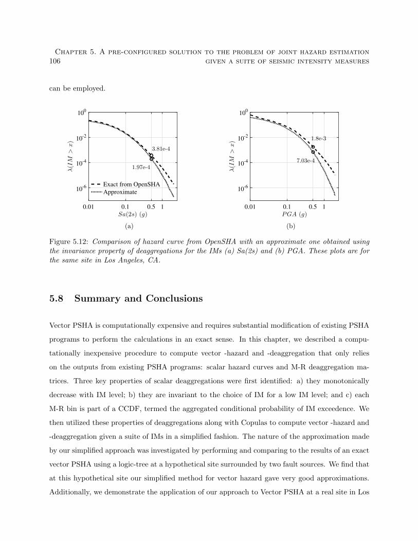
106Chapter 5. A pre-configured solution to the problem of joint hazard estimation
given a suite of seismic intensity measures
can be employed.
0.01 0.1 0.5 1
Sa(2s) (g)
10-6
10-4
10-2
100
λ(IM
>x)
Exact from OpenSHA
Approximate
1.97e-4
3.81e-4
(a)
0.01 0.1 0.5 1
PGA (g)
10-6
10-4
10-2
100
λ(IM
>x) 1.8e-3
7.03e-4
(b)
Figure 5.12: Comparison of hazard curve from OpenSHA with an approximate one obtained usingthe invariance property of deaggregations for the IMs (a) Sa(2s) and (b) PGA. These plots are forthe same site in Los Angeles, CA.
5.8 Summary and Conclusions
Vector PSHA is computationally expensive and requires substantial modification of existing PSHA
programs to perform the calculations in an exact sense. In this chapter, we described a compu-
tationally inexpensive procedure to compute vector -hazard and -deaggregation that only relies
on the outputs from existing PSHA programs: scalar hazard curves and M-R deaggregation ma-
trices. Three key properties of scalar deaggregations were first identified: a) they monotonically
decrease with IM level; b) they are invariant to the choice of IM for a low IM level; and c) each
M-R bin is part of a CCDF, termed the aggregated conditional probability of IM exceedence. We
then utilized these properties of deaggregations along with Copulas to compute vector -hazard and
-deaggregation given a suite of IMs in a simplified fashion. The nature of the approximation made
by our simplified approach was investigated by performing and comparing to the results of an exact
vector PSHA using a logic-tree at a hypothetical site surrounded by two fault sources. We find that
at this hypothetical site our simplified method for vector hazard gave very good approximations.
Additionally, we demonstrate the application of our approach to Vector PSHA at a real site in Los
5.8. Summary and Conclusions 107
Angeles, CA, using the PSHA program OpenSHA.
Our approach for simplified computation of vector PSHA accounts for logic-tree and multiple
fault sources (routinely considered in modern PSHA computations) while taking as inputs only the
basic quantities such as scalar hazard curve and M-R deaggregations. As a result, we anticipate
that our method will be valuable given that modern GMPMs may account for more fault-specific
parameters and PSHA may consider more epistemic uncertainty through logic-tree in the future.
Finally, we also provide a discussion on how the invariance property of deaggregations can be
used to compute hazard curves for new GMPMs or GMPMs fitted to new IMs. The computed
hazard curve is only exact if a single GMPM is used in logic trees and this GMPM does not
account for earthquake source related parameters. However, for the IMs and the site considered in
this study, we obtain reasonable predictions for low to moderate values of the IM.

Chapter 6
A Bayesian treatment of the
Conditional Spectrum approach for
ground motion selection
This chapter expands upon a study excerpted from:
Somayajulu L.N. Dhulipala and Madeleine M. Flint. “Bayesian Conditional Spectrum for Ground
Motion Selection” Earthquake Engineering and Structural Dynamics (under review).
6.1 Introduction
Selection of appropriate ground motions is a crucial aspect in seismic response analysis of struc-
tures. Accelerogram selection is often made by matching the selected motions to a target response
spectrum such as the Uniform Hazard Spectrum (UHS) or the Conditional Mean Spectrum (CMS).
The UHS can be preferred when seismic vulnerability of communities is of interest, a case where
the properties of buildings, e.g., the fundamental time period, are variable. When the seismic
vulnerability of a single building/facility is of interest, the UHS is shown to be conservative, and
the CMS was developed as a more reasonable ground motion selection target (Baker and Cornell,
2006). The CMS was developed from the observation that εs (normalized ground motion residuals)
across the spectral time periods are correlated and this correlation influences the spectral shape
(Baker and Cornell, 2006). Baker (2010)Baker (2011) formalized the CMS based on ε (CMS-ε)
and also emphasized the criticality of accounting for the variability around the CMS resulting due
to the dispersion of a Ground Motion Prediction Model (GMPM). The CMS and the Conditional
standard deviation around it are jointly referred to as the Conditional Spectrum (CS).
108
6.1. Introduction 109
Many additions and modifications have been proposed to the CS over the years. For exam-
ple, Bradley (2010)Bradley (2010b) proposes a holistic ground motion selection methodology by
extending the CS to include non-spectral Intensity Measures (IM) such as Peak Ground Accelera-
tion and Velocity (PGA, PGV). Carlton and Abrahamson (2014)Carlton and Abrahamson (2014)
explore some issues related to the CMS which include broadening the CMS to match the UHS
with fewer conditioning periods and investigating the robustness of the correlation coefficients used
in calculations. Chandramohan et al. (2016)Chandramohan et al. (2016) select ground motions
to match the conditional distribution of 5 − 75% significant duration (Ds575) conditioned on the
structure’s fundamental time period in order to investigate the influence of ground motion duration
on structural collapse. More recently, Kohrangi et al.(2017)Kohrangi et al. (2017) extend the CS to
include average spectral acceleration, an IM which has been demonstrated to be a good predictor
of multiple Engineering Demand Parameters (EDP) that are considered in risk assessment of a
structure.
In this chapter, we cast the CS into a Bayesian framework. A Bayesian inference can be argued
to be a generalization of a Frequentist inference1. Whereas a Frequentist treatment fits models given
data, a Bayesian treatment, while having the capability to do the same, also provides a mechanism
to update the models in light of new information or changing preferences of the analysts. This is
because, a Frequentist’s philosophy is that there exists some underlying, true model parameters
and it is the data which is random, whereas, a Bayesian’s philosophy is that the inferred model
parameters are opinions given a data-set and these opinions can change. In other words, a Bayesian
approach is, in a sense, more “flexible” than a Frequentist approach, but also is, at the same time,
capable of reproducing the Frequentist results under certain input conditions; a detailed discussion
of this is provided further in this chapter. Furthermore, the mathematical framework of a Bayesian
treatment allows accounting for other preferences of an analyst specific to their site or structure
under consideration. We employ a Bayesian method to simulate the CMS and the Conditional
standard deviation, and explore three advantages that this method offers:
1. Consideration of multiple causal events. A Bayesian procedure implicitly accounts for
the variability in deaggregation Magnitude (M)-Distance (R) pairs contributing to a given
1Treatment of the CS in previous literature is considered to be a Frequentist treatment.
110Chapter 6. A Bayesian treatment of the Conditional Spectrum approach for
ground motion selection
level of seismic hazard. I.e., the analyst need not select just one M -R pair, as is common in
the traditional CS approach.
2. Incorporation of additional information using the prior distributions. It is possible
to simulate the CS using only a preferred population of ground motions by adjusting the
prior distributions in a Bayesian model. For example an analyst interested in large M -small
R might use simulated ground motions to construct the prior distributions, which can then
be combined with a likelihood function reflecting the real ground motion data.
3. Multiple IMs are treated holistically. The Bayesian approach is supported by vector-
based (i.e., multi-IM) hazard analysis and deaggregation. It is therefore possible to extend
the CS to a general class of structures by conditioning on single/multiple IMs (spectral or
non-spectral) as dictated by the structural type and its sensitivity to different ground motion
aspects. Such a consideration of non-spectral IMs shares similarities with the Generalized
Conditioning Intensity Measure approach (Bradley, 2010b), although the Bayesian approach
is additionally capable of conditioning on multiple IMs.
The Bayesian CS is introduced in Section 6.2 and its equivalence to the traditional CS-ε is
demonstrated. Section 6.3 discusses how a Bayesian CS is capable of implicitly considering multiple
values of the causal parameters (M − R) from the deaggregation plot. The influence of such a
consideration on the CS is demonstrated at sites in Los Angeles, Bissell, and Stanford. The use of
simulated priors combined with high-risk ground motion data is performed and the consequences
concerning the CS are explored in Section 6.4. Finally, the motivation for conditioning on multiple
IMs is discussed and its impact on the CS is investigated in Section 6.5.
6.2 Bayesian Conditional Spectrum
In this section, we discuss some preliminaries related to ground motion modeling and demonstrate
the Bayesian CS and its equivalence to the traditional CS.
6.2. Bayesian Conditional Spectrum 111
6.2.1 Ground motion modeling
Empirical equation of the ground motion model
A Bayesian treatment of the CS starts with the ground motion model. We adopt a ground motion
model similar to that by Boore et al. (2008)Boore and Atkinson (2008) consisting of source, path,
and site terms,
ln(yij) = FE(Mi,mechi) + FP (RJB,i,Mi, regioni) + FS(V s30,i) + εij σj (6.1)
where yij is the predicted value of the ith ground motion at jth spectral period; FE , FP and
FS are the source, path and site terms, respectively; M is the earthquake magnitude, mech is the
source mechanism, RJB is the Joyner-Boore distance and V s30 is the shear wave velocity averaged
over the top 30 meters depth; σj is the standard deviation in predicting the ground motion at jth
spectral period and εij is the number of standard deviations required to accurately predict the ith
ground motion observation at jth spectral period. The source, path and site terms of the model
are further expanded as,
FE(M,mech) =
e0U + e1SS + e2NS + e3RS + e4(M −Mh) + e5(M −Mh)2, M ≤Mh
e0U + e1SS + e2NS + e3RS + e6(M −Mh), otherwise
(6.2)
FP (RJb,M, region) = [c1+c2(M−Mref )]ln(R/Rref )+c3(R−Rref ) (where R =√R2JB + h2) (6.3)
FS(V s30) = blin ln(V s30/Vref ) (6.4)
where ek, ck, blin, and h are the model coefficients; Mh is the hinge magnitude; Mref , Rref
and Vref are the reference magnitude, distance and shear velocity, respectively; U , SS, NS and RS
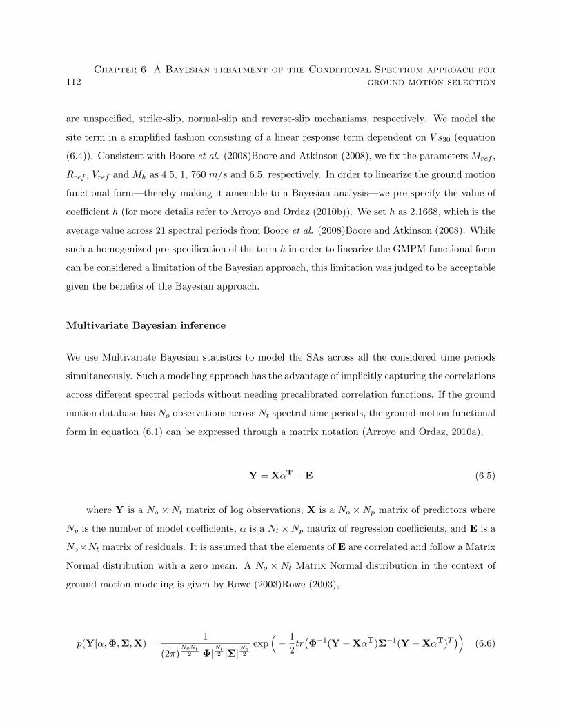
112Chapter 6. A Bayesian treatment of the Conditional Spectrum approach for
ground motion selection
are unspecified, strike-slip, normal-slip and reverse-slip mechanisms, respectively. We model the
site term in a simplified fashion consisting of a linear response term dependent on V s30 (equation
(6.4)). Consistent with Boore et al. (2008)Boore and Atkinson (2008), we fix the parameters Mref ,
Rref , Vref and Mh as 4.5, 1, 760 m/s and 6.5, respectively. In order to linearize the ground motion
functional form—thereby making it amenable to a Bayesian analysis—we pre-specify the value of
coefficient h (for more details refer to Arroyo and Ordaz (2010b)). We set h as 2.1668, which is the
average value across 21 spectral periods from Boore et al. (2008)Boore and Atkinson (2008). While
such a homogenized pre-specification of the term h in order to linearize the GMPM functional form
can be considered a limitation of the Bayesian approach, this limitation was judged to be acceptable
given the benefits of the Bayesian approach.
Multivariate Bayesian inference
We use Multivariate Bayesian statistics to model the SAs across all the considered time periods
simultaneously. Such a modeling approach has the advantage of implicitly capturing the correlations
across different spectral periods without needing precalibrated correlation functions. If the ground
motion database has No observations across Nt spectral time periods, the ground motion functional
form in equation (6.1) can be expressed through a matrix notation (Arroyo and Ordaz, 2010a),
Y = XαT + E (6.5)
where Y is a No ×Nt matrix of log observations, X is a No ×Np matrix of predictors where
Np is the number of model coefficients, α is a Nt ×Np matrix of regression coefficients, and E is a
No×Nt matrix of residuals. It is assumed that the elements of E are correlated and follow a Matrix
Normal distribution with a zero mean. A No × Nt Matrix Normal distribution in the context of
ground motion modeling is given by Rowe (2003)Rowe (2003),
p(Y|α,Φ,Σ,X) =1
(2π)NoNt
2 |Φ|Nt2 |Σ|
No2
exp(− 1
2tr(Φ−1(Y −XαT)Σ−1(Y −XαT)T
))(6.6)
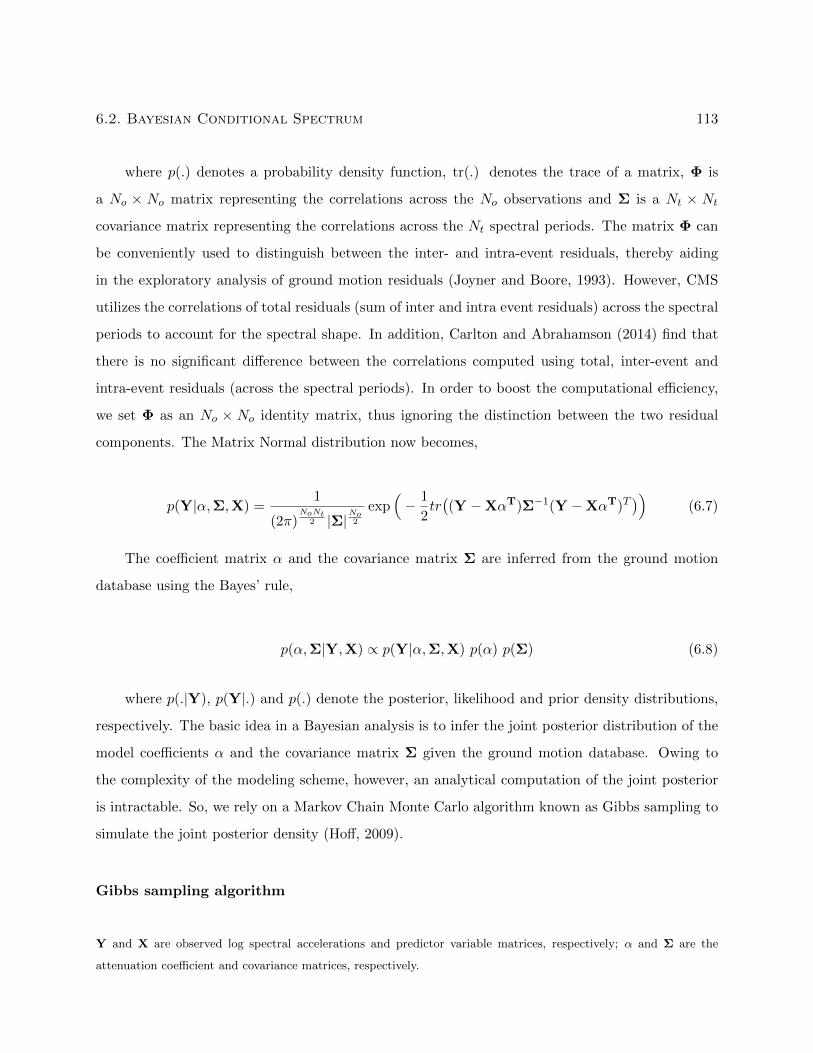
6.2. Bayesian Conditional Spectrum 113
where p(.) denotes a probability density function, tr(.) denotes the trace of a matrix, Φ is
a No × No matrix representing the correlations across the No observations and Σ is a Nt × Nt
covariance matrix representing the correlations across the Nt spectral periods. The matrix Φ can
be conveniently used to distinguish between the inter- and intra-event residuals, thereby aiding
in the exploratory analysis of ground motion residuals (Joyner and Boore, 1993). However, CMS
utilizes the correlations of total residuals (sum of inter and intra event residuals) across the spectral
periods to account for the spectral shape. In addition, Carlton and Abrahamson (2014) find that
there is no significant difference between the correlations computed using total, inter-event and
intra-event residuals (across the spectral periods). In order to boost the computational efficiency,
we set Φ as an No × No identity matrix, thus ignoring the distinction between the two residual
components. The Matrix Normal distribution now becomes,
p(Y|α,Σ,X) =1
(2π)NoNt
2 |Σ|No2
exp(− 1
2tr((Y −XαT)Σ−1(Y −XαT)T
))(6.7)
The coefficient matrix α and the covariance matrix Σ are inferred from the ground motion
database using the Bayes’ rule,
p(α,Σ|Y,X) ∝ p(Y|α,Σ,X) p(α) p(Σ) (6.8)
where p(.|Y), p(Y|.) and p(.) denote the posterior, likelihood and prior density distributions,
respectively. The basic idea in a Bayesian analysis is to infer the joint posterior distribution of the
model coefficients α and the covariance matrix Σ given the ground motion database. Owing to
the complexity of the modeling scheme, however, an analytical computation of the joint posterior
is intractable. So, we rely on a Markov Chain Monte Carlo algorithm known as Gibbs sampling to
simulate the joint posterior density (Hoff, 2009).
Gibbs sampling algorithm
Y and X are observed log spectral accelerations and predictor variable matrices, respectively; α and Σ are the
attenuation coefficient and covariance matrices, respectively.
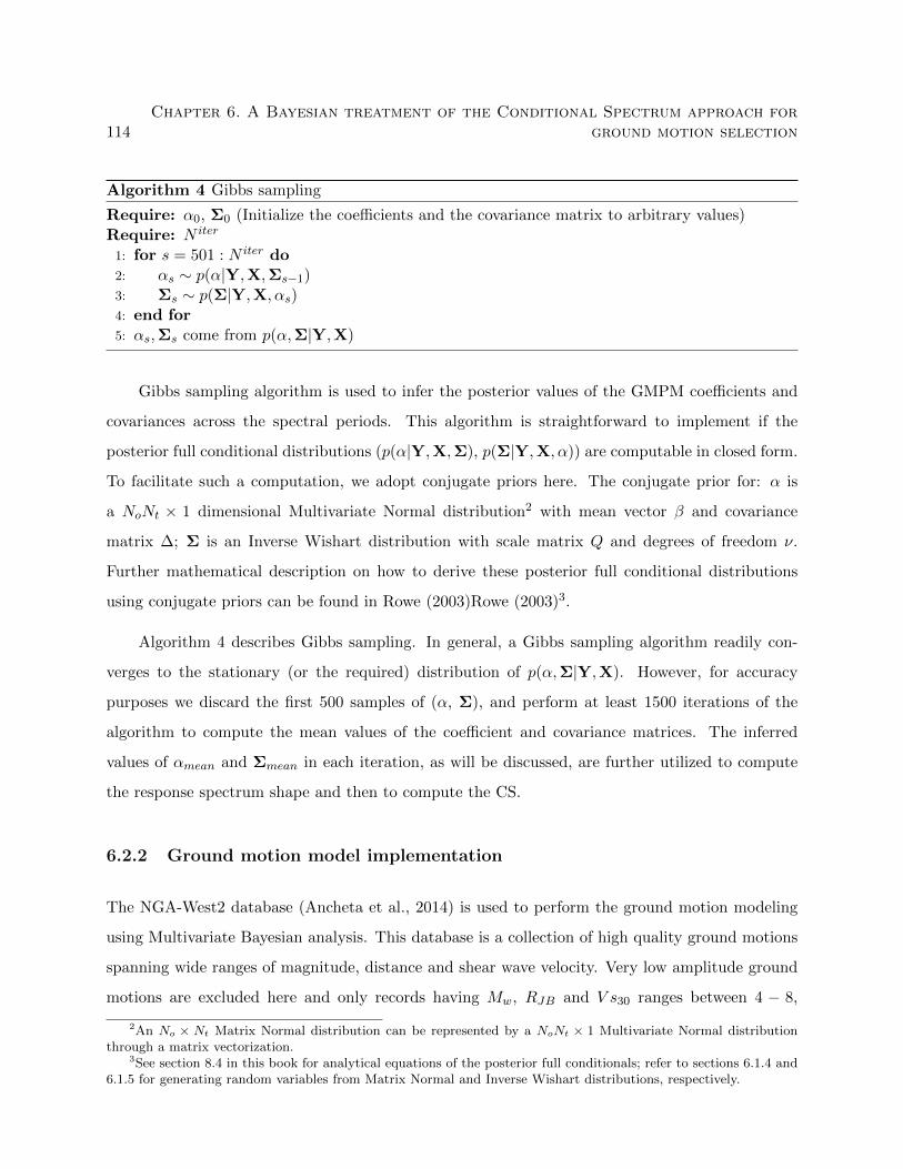
114Chapter 6. A Bayesian treatment of the Conditional Spectrum approach for
ground motion selection
Algorithm 4 Gibbs sampling
Require: α0, Σ0 (Initialize the coefficients and the covariance matrix to arbitrary values)Require: N iter
1: for s = 501 : N iter do2: αs ∼ p(α|Y,X,Σs−1)3: Σs ∼ p(Σ|Y,X, αs)4: end for5: αs,Σs come from p(α,Σ|Y,X)
Gibbs sampling algorithm is used to infer the posterior values of the GMPM coefficients and
covariances across the spectral periods. This algorithm is straightforward to implement if the
posterior full conditional distributions (p(α|Y,X,Σ), p(Σ|Y,X, α)) are computable in closed form.
To facilitate such a computation, we adopt conjugate priors here. The conjugate prior for: α is
a NoNt × 1 dimensional Multivariate Normal distribution2 with mean vector β and covariance
matrix ∆; Σ is an Inverse Wishart distribution with scale matrix Q and degrees of freedom ν.
Further mathematical description on how to derive these posterior full conditional distributions
using conjugate priors can be found in Rowe (2003)Rowe (2003)3.
Algorithm 4 describes Gibbs sampling. In general, a Gibbs sampling algorithm readily con-
verges to the stationary (or the required) distribution of p(α,Σ|Y,X). However, for accuracy
purposes we discard the first 500 samples of (α, Σ), and perform at least 1500 iterations of the
algorithm to compute the mean values of the coefficient and covariance matrices. The inferred
values of αmean and Σmean in each iteration, as will be discussed, are further utilized to compute
the response spectrum shape and then to compute the CS.
6.2.2 Ground motion model implementation
The NGA-West2 database (Ancheta et al., 2014) is used to perform the ground motion modeling
using Multivariate Bayesian analysis. This database is a collection of high quality ground motions
spanning wide ranges of magnitude, distance and shear wave velocity. Very low amplitude ground
motions are excluded here and only records having Mw, RJB and V s30 ranges between 4 − 8,
2An No × Nt Matrix Normal distribution can be represented by a NoNt × 1 Multivariate Normal distributionthrough a matrix vectorization.
3See section 8.4 in this book for analytical equations of the posterior full conditionals; refer to sections 6.1.4 and6.1.5 for generating random variables from Matrix Normal and Inverse Wishart distributions, respectively.

6.2. Bayesian Conditional Spectrum 115
1 − 200Km, and 100 − 2000m/s, respectively, are considered. Imposing these restrictions, the
NGA-West2 database is curtailed here to have No = 4390 recordings from Ne = 212 earthquakes
across Nt = 26 spectral time periods that are evenly distributed in a log-space between 0.1 and 5
seconds.
The Gibbs sampling algorithm is then implemented to infer the posterior model coefficients
and the covariance matrix from the curtailed database using non-informative prior distributions
on α and Σ. The prior distributions p(α) and p(Σ) do not contribute towards ground motion
modeling if their corresponding covariance (∆) and scale (Q) matrices, respectively, are diffuse
(i.e. the elements in these matrices are numerically large). More description on the choice of prior
distributions will be provided in section 6.4 of this chapter. The model coefficients inferred using
Gibbs sampling are utilized to predict the SAs in the curtailed database.
6.2.3 Conditioning at a spectral time period
In this section, conditioning of the response spectrum is made by specifying the SA value at a time
period. The mean response spectrum (CMS) and the variability around it (Conditional standard
deviation) are then simulated.
Multivariate Normal distribution theory
A Bayesian ground motion model can simulate the means of the model coefficients and the covari-
ance matrix. Given a set of Mw, RJB, V s30, and fault-type parameters, the log response spectrum
for each iteration of the Gibbs sampling algorithm can be computed using,
[µlnSa(Ti)
]s = αsX (6.9)
where Ti is the ith spectral time period and X is a Np × 1 vector of source/site parameters.
The conditional mean vector and the conditional covariance matrix given the SAs at N∗ time
periods (where N∗ periods are a subset of the total time periods considered) can be computed
using Multivariate Normal distribution theory,
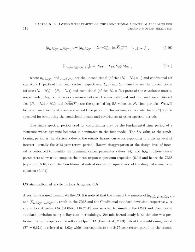
116Chapter 6. A Bayesian treatment of the Conditional Spectrum approach for
ground motion selection
[µlnSa(Ti)|lnSa(T ∗)
]s =[µlnSa(Ti)
+ ΣUCΣ−1CC (lnSa(T ∗)− µlnSa(T ∗)
)]s
(6.10)
[ΣlnSa(Ti)|lnSa(T ∗)
]s =[ΣUU − ΣUCΣ−1CCΣT
UC
]s
(6.11)
where µlnSa(Ti)
and µlnSa(T∗) are the unconditional (of size (Nt −N∗)× 1) and conditional (of
size N∗ × 1) parts of the mean vector, respectively; ΣCC and ΣUU are the are the unconditional
(of size (Nt −N∗) × (Nt −N∗)) and conditional (of size N∗ ×N∗) parts of the covariance matrix,
respectively; ΣUC is the cross covariance between the unconditional and the conditional SAs (of
size (Nt − N∗) × N∗); and lnSa(T ∗) are the specified log SA values at N∗ time periods. We will
focus on conditioning at a single spectral time period in this section, i.e., a scalar lnSa(T ∗) will be
specified for computing the conditional means and covariances at other spectral periods.
The single spectral period used for conditioning may be the fundamental time period of a
structure whose dynamic behavior is dominated in the first mode. The SA value at the condi-
tioning period is the abscissa value of the seismic hazard curve corresponding to a design level of
interest—usually the 2475 year return period. Hazard deaggregation at the design level of inter-
est is performed to identify the dominant causal parameter values (Mw and RJB). These causal
parameters allow us to compute the mean response spectrum (equation (6.9)) and hence the CMS
(equation (6.10)) and the Conditional standard deviation (square root of the diagonal elements in
equation (6.11)).
CS simulation at a site in Los Angeles, CA
Algorithm 5 is used to simulate the CS. It is noticed that the mean of the samples of [µlnSa(Ti)|lnSa(T ∗)
]s
and [ΣlnSa(Ti)|lnSa(T ∗)
]s result in the CMS and the Conditional standard deviation, respectively. A
site in Los Angeles, CA [34.05N, 118.25W ] was selected to simulate the CMS and Conditional
standard deviation using a Bayesian methodology. Seismic hazard analysis at this site was per-
formed using the open-source software OpenSHA (Field et al., 2003). SA at the conditioning period
(T ∗ = 0.67s) is selected as 1.02g which corresponds to the 2475-year return period on the seismic
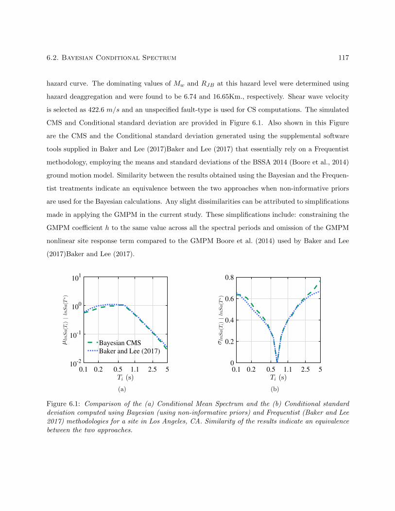
6.2. Bayesian Conditional Spectrum 117
hazard curve. The dominating values of Mw and RJB at this hazard level were determined using
hazard deaggregation and were found to be 6.74 and 16.65Km., respectively. Shear wave velocity
is selected as 422.6 m/s and an unspecified fault-type is used for CS computations. The simulated
CMS and Conditional standard deviation are provided in Figure 6.1. Also shown in this Figure
are the CMS and the Conditional standard deviation generated using the supplemental software
tools supplied in Baker and Lee (2017)Baker and Lee (2017) that essentially rely on a Frequentist
methodology, employing the means and standard deviations of the BSSA 2014 (Boore et al., 2014)
ground motion model. Similarity between the results obtained using the Bayesian and the Frequen-
tist treatments indicate an equivalence between the two approaches when non-informative priors
are used for the Bayesian calculations. Any slight dissimilarities can be attributed to simplifications
made in applying the GMPM in the current study. These simplifications include: constraining the
GMPM coefficient h to the same value across all the spectral periods and omission of the GMPM
nonlinear site response term compared to the GMPM Boore et al. (2014) used by Baker and Lee
(2017)Baker and Lee (2017).
0.1 0.2 0.5 1.1 2.5 5Ti (s)
10-2
10-1
100
101
µlnSa(T
i)|lnSa(T
∗)
Bayesian CMS
Baker and Lee (2017)
(a)
0.1 0.2 0.5 1.1 2.5 5
Ti (s)
0
0.2
0.4
0.6
0.8
σlnSa(T
i)|lnSa(T
∗)
(b)
Figure 6.1: Comparison of the (a) Conditional Mean Spectrum and the (b) Conditional standarddeviation computed using Bayesian (using non-informative priors) and Frequentist (Baker and Lee2017) methodologies for a site in Los Angeles, CA. Similarity of the results indicate an equivalencebetween the two approaches.
118Chapter 6. A Bayesian treatment of the Conditional Spectrum approach for
ground motion selection
6.3 Accounting for the M-R pair selection uncertainty from the
deaggregation plot
Computing the CS requires a mean prediction of the response spectrum from the ground motion
model, with inputs including the causal parameters M-R. The traditional technique to stipulate
these causal parameters is to consider the mean or mode M-R pair obtained from the deaggregation
given the hazard level of the conditioning IM. Deaggregations, in general, have probability masses
concentrated across several M-R bins depending upon the site, IM, and hazard level chosen. Lin et
al. (2013)Lin et al. (2013a) explore the effects of considering several possible values of M-R on CS
computations and find that such a consideration leads to a more exact representation of the CMS
and the Conditional standard deviation. These authors use a Frequentist approach to compute the
CS and use analytical equations to propagate the variability of M-R within a deaggregation plot to
the CS. Alternatively, the Bayesian approach presented here has an inherent capacity to simulate
the CS considering a random pair of M-R during each iteration; M-R pairs are randomly drawn in
proportion to a given deaggregation probability matrix. The CMS and the Conditional standard
deviation thus computed reflect not only the uncertainty in ground motion modeling but also the
randomness in determining an M-R pair from the deaggregation. The Bayesian procedure for this
case is also described by Algorithm 5.
Algorithm 5 CS simulation with the Gibbs sampling algorithm
Require: α0, Σ0 (Initialize the coefficients and the covariance matrix to arbitrary values)Require: N iter
Require: Target SA at the conditioning period and deaggregation matrix from hazard analysis1: for s = 501 : N iter do2: αs ∼ p(α|Y,X,Σs−1)3: Σs ∼ p(Σ|Y,X, αs)4: [MR]⇐ mean values from deaggregation matrix (can be set to random values drawn from
the deaggregation matrix as well)5: [µ
lnSa(Ti)]s = αsX
6: Compute [µlnSa(Ti)|lnSa(T ∗)
]s from equation (6.10)
7: Compute [ΣlnSa(Ti)|lnSa(T ∗)
]s from equation (6.11)
8: end for9: CMS ⇐ mean([µ
lnSa(Ti)|lnSa(T ∗)]s)
10: Conditional standard deviation⇐ sqrt(mean([Σ
lnSa(Ti)|lnSa(T ∗)]s))
(only the diagonal elements
are considered)
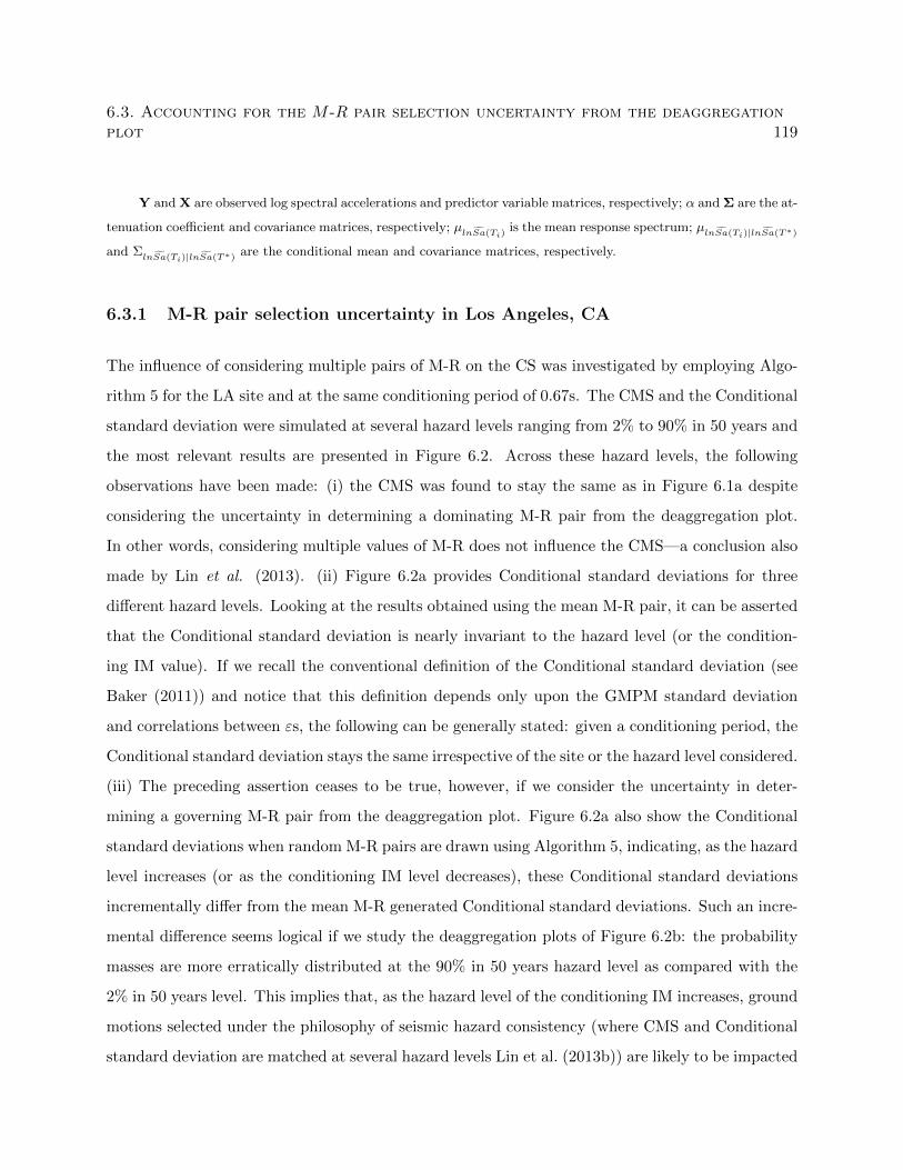
6.3. Accounting for the M-R pair selection uncertainty from the deaggregationplot 119
Y and X are observed log spectral accelerations and predictor variable matrices, respectively; α and Σ are the at-
tenuation coefficient and covariance matrices, respectively; µlnSa(Ti)is the mean response spectrum; µlnSa(Ti)|lnSa(T∗)
and ΣlnSa(Ti)|lnSa(T∗) are the conditional mean and covariance matrices, respectively.
6.3.1 M-R pair selection uncertainty in Los Angeles, CA
The influence of considering multiple pairs of M-R on the CS was investigated by employing Algo-
rithm 5 for the LA site and at the same conditioning period of 0.67s. The CMS and the Conditional
standard deviation were simulated at several hazard levels ranging from 2% to 90% in 50 years and
the most relevant results are presented in Figure 6.2. Across these hazard levels, the following
observations have been made: (i) the CMS was found to stay the same as in Figure 6.1a despite
considering the uncertainty in determining a dominating M-R pair from the deaggregation plot.
In other words, considering multiple values of M-R does not influence the CMS—a conclusion also
made by Lin et al. (2013). (ii) Figure 6.2a provides Conditional standard deviations for three
different hazard levels. Looking at the results obtained using the mean M-R pair, it can be asserted
that the Conditional standard deviation is nearly invariant to the hazard level (or the condition-
ing IM value). If we recall the conventional definition of the Conditional standard deviation (see
Baker (2011)) and notice that this definition depends only upon the GMPM standard deviation
and correlations between εs, the following can be generally stated: given a conditioning period, the
Conditional standard deviation stays the same irrespective of the site or the hazard level considered.
(iii) The preceding assertion ceases to be true, however, if we consider the uncertainty in deter-
mining a governing M-R pair from the deaggregation plot. Figure 6.2a also show the Conditional
standard deviations when random M-R pairs are drawn using Algorithm 5, indicating, as the hazard
level increases (or as the conditioning IM level decreases), these Conditional standard deviations
incrementally differ from the mean M-R generated Conditional standard deviations. Such an incre-
mental difference seems logical if we study the deaggregation plots of Figure 6.2b: the probability
masses are more erratically distributed at the 90% in 50 years hazard level as compared with the
2% in 50 years level. This implies that, as the hazard level of the conditioning IM increases, ground
motions selected under the philosophy of seismic hazard consistency (where CMS and Conditional
standard deviation are matched at several hazard levels Lin et al. (2013b)) are likely to be impacted
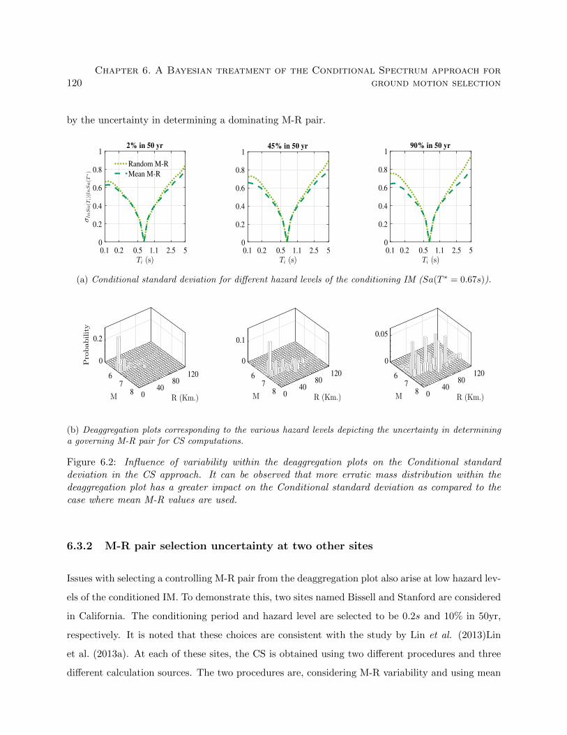
120Chapter 6. A Bayesian treatment of the Conditional Spectrum approach for
ground motion selection
by the uncertainty in determining a dominating M-R pair.
0.1 0.2 0.5 1.1 2.5 5
Ti (s)
0
0.2
0.4
0.6
0.8
1
σlnSa(T
i)|lnSa(T
∗)
2% in 50 yr
Random M-R
Mean M-R
0.1 0.2 0.5 1.1 2.5 5
Ti (s)
0
0.2
0.4
0.6
0.8
145% in 50 yr
0.1 0.2 0.5 1.1 2.5 5
Ti (s)
0
0.2
0.4
0.6
0.8
190% in 50 yr
(a) Conditional standard deviation for different hazard levels of the conditioning IM (Sa(T ∗ = 0.67s)).
0Probability
0.2
1206
M
80
R (Km.)
740
8 0
0
0.1
1206
M
80
R (Km.)
740
8 0
0
120
0.05
6
M
80
R (Km.)
740
8 0
(b) Deaggregation plots corresponding to the various hazard levels depicting the uncertainty in determininga governing M-R pair for CS computations.
Figure 6.2: Influence of variability within the deaggregation plots on the Conditional standarddeviation in the CS approach. It can be observed that more erratic mass distribution within thedeaggregation plot has a greater impact on the Conditional standard deviation as compared to thecase where mean M-R values are used.
6.3.2 M-R pair selection uncertainty at two other sites
Issues with selecting a controlling M-R pair from the deaggregation plot also arise at low hazard lev-
els of the conditioned IM. To demonstrate this, two sites named Bissell and Stanford are considered
in California. The conditioning period and hazard level are selected to be 0.2s and 10% in 50yr,
respectively. It is noted that these choices are consistent with the study by Lin et al. (2013)Lin
et al. (2013a). At each of these sites, the CS is obtained using two different procedures and three
different calculation sources. The two procedures are, considering M-R variability and using mean
6.3. Accounting for the M-R pair selection uncertainty from the deaggregationplot 121
M-R pair from the deaggregation plot. The three calculation sources are, Bayesian method of this
study, Frequentist method of Lin et al. (2013)Lin et al. (2013a) using the BSSA 2014 GMPM, and
data from Lin et al. (2013)Lin et al. (2013a). It is noted that the data from Lin et al. (2013)Lin
et al. (2013a) relies on three NGA-West1 GMPMs for making the CS computations. For a given site
and procedure, all three sources for CS calculations resulted in quite consistent CMSs, so further
discussion concerning this will not be made.
The Conditional standard deviations, although being consistent between the calculation sources
when mean M-R values are used from the deaggregation plots (see Figures 6.3a and 6.3b), demon-
strated some dissimilarity when M-R variability within these plots is additionally considered (see
Figures 6.3c and 6.3d). Such inconsistencies between calculation sources under this procedure con-
sidering M-R variability can attributed to two causes: (1) differences between the ground motion
data sources used and (2) differences between GMPM functional forms adopted.
First, the study by Lin et al. (2013)Lin et al. (2013a) at its core, through the GMPMs, relies
on the NGA-West 1 database for making the CS computations. Although the Bayesian calculations
use the NGA-West 2 database, the processing of this database adopted in this study is slightly at
odds with what was adopted for the development of BSSA 2014. These differences are expected to
contribute to the deviations between Conditional standard deviations presented in Figures 6.3c and
6.3d not only through changes in the unconditional standard deviations of the predicted spectral
intensities, but also through changes in the correlations between spectral periods. Despite this, the
Conditional standard deviation obtained from Bayesian calculations is consistent with the BSSA
2014 Frequentist calculations at large spectral periods in Figure 6.3c4. As an aside, the flexibility
offered by a Bayesian in terms of using a ground motion database of the analyst’s preference has
important implications, and these are discussed in the subsequent section.
Second, the study by Lin et al. (2013)Lin et al. (2013a), through GMPM deaggregation, uses
four NGA GMPMs to calculate the Conditional standard deviations presented in Figures 6.3c and
6.3d. The Bayesian calculations rely on a simplified functional form of the BSSA 2014 GMPM.
4It is noted that the Frequentist approach for considering M-R variability within deaggregation plots itself is notresponsible for the differences in the results. This is because, when using the curtailed NGA-West2 dataset for fittingthe GMPM functional form of equation (6.1), a Frequentist procedure for considering M-R variability resulted in thesame Conditional standard deviation as with a Bayesian approach.

122Chapter 6. A Bayesian treatment of the Conditional Spectrum approach for
ground motion selection
These differences in the GMPM functional forms are additionally expected to contribute to the
differences in Conditional standard deviations presented in Figures 6.3c and 6.3d. Evidence for
these expected differences come from prior work. Gregor et al. (2014)Gregor et al. (2014) (especially
in Figures 8 and 9) compared the NGA-West2 GMPM functional forms and identified differences
between the predicted response spectral shapes for several magnitude-distance combinations.
6.4 Effects of tuning the priors to simulated ground motions on
the Conditional Spectrum
6.4.1 Motivation
In the previous sections, non-informative (or diffuse) priors were used in the Bayesian methodology
to simulate the CS. The priors in the Bayesian approach are beliefs about ground motion amplitudes,
their dependence on the rupture parameters, and their attenuation. The utilization of flat priors
implies that the analyst does not hold any beliefs on ground motions and their characteristics
before observing real data. Such a modeling approach is similar to that of a Frequentist approach
where prior knowledge about a phenomenon, possibly subjective, is disregarded in the analysis.
The ability of a Bayesian approach to give credit to these prior beliefs of an analyst is what makes
this approach flexible and general.
While prior beliefs might take the form of constraining or guessing the coefficient values by
using appropriate probability distributions, the primary foreseen application is the use of simulated
ground motions. With the rapid development of ground motion simulations, there will be no
shortage of beliefs on the earthquake processes and their consequences. In other words, the priors
in the Bayesian approach can be tuned to represent certain simulated earthquake characteristics
that are important for seismic risk analysis and which may not be available in abundance in the
recorded ground motion database.
Examples of these earthquake characteristics for which the simulated priors can be tuned may
include: (1) large magnitude-small distance records; (2) pulse-like ground motions; and (3) ground
motions pertaining to specific fault sources that are identified to dominate the seismic hazard at a
6.4. Effects of tuning the priors to simulated ground motions on the ConditionalSpectrum 123
site. Such a tuning of priors allows analysts to draw inference from both observed as well as simu-
lated ground motions in a manner that is both logical and philosophically acceptable. A procedural
illustration of tuning the priors to simulated ground motions will be presented accompanied by a
numerical example.
6.4.2 High risk ground motions in the NGA-West2 database
Large magnitude-small distance records (or, high-risk ground motions), despite entailing consider-
able engineering interest, amount to a very small fraction of the curtailed NGA-West2 database.
For example, Mw > 6.5 and RJB < 20Km records contribute to only 5.7% (250 records) of the
curtailed NGA-West2 database. Even within this subset, motions that are M > 7.1, as observed
from Figure 6.4a, are sparsely populated. Therefore, the CS computations made thus far relied
heavily on combinations of small/medium magnitude and moderate/large distance earthquakes.
The existence of an adequate number of large magnitude-small distance records becomes impor-
tant for making reliable CS computations at sites where the seismic hazard is high. For example,
the LA and Stanford sites have Sa(0.67s) for a return period of 2475 years as 1.02g and 1.79g,
respectively; the Stanford site has a mean M−R combination at this hazard level as 7.56−7.42Km.
Ground motion simulations will be used to augment the Mw > 6.5 and RJB < 20Km NGA-West2
subset wherein, the Bayes rule(equation (6.8)
)will serve as a bridge between the observed and the
simulated datasets.
6.4.3 Simulation of high-risk ground motions
Techniques and tools for simulating ground motions are rapidly developing with the broader goal
of providing more insight into the earthquake process and more control to the analysts without
having to completely rely on recorded ground motions. Simulation methods vary with regard to
the complexity they use in treating the earthquake process. EXSIM falls into the category of finite-
fault stochastic methods in which Fourier spectra derived using earthquake physics are inverted to
simulate accelerograms. Graves and PitarkaGraves and Pitarka (2015) and UCSB Crempien and
Archuleta (2015) methods fall into the category of hybrid techniques where both stochastic inversion

124Chapter 6. A Bayesian treatment of the Conditional Spectrum approach for
ground motion selection
of Fourier spectra and deterministic wave propagation effects are used to simulate accelerograms.
Furthermore, the Southern California Earthquake Center is developing a database of simulated
ground motions (for example see Goulet et al. (2018)) which is expected to be of great practical as
it does not require analysts to conduct their own simulations.
While ground motion simulations are finding many applications in seismic hazard and risk
analysis (for e.g., see Graves et al. 2011Graves et al. (2011) and Bijelic et al. 2018Bijelic et al.
(2018)), the limits of such simulations should also be noted. For example, Dreger et al. (2015)Dreger
et al. (2015) validate some ground motion simulation methods by contrasting them with recorded
motions. Their study finds that simulated motions, while being generally satisfactory, are more
representative of real records for short period ranges than for longer periods (> 3s). In addition,
these simulation methods are mostly validated against data from active crustal regions (e.g., Cali-
fornia) rather than for stable continental regions (e.g., Eastern North America). The use of ground
motion simulations within a Bayesian framework should therefore include careful consideration of
the limitations of simulated ground motions.
For the purposes of illustration, the highly computationally efficient EXSIM (Motazedian and
Atkinson, 2005) is utilized for simulating ground motions resulting from earthquakes with M >
6.5. EXSIM is a stochastic finite-fault based ground motion simulation program (Motazedian and
Atkinson, 2005) that divides the entire rupture area into a number of sub-faults, treating each of
these subdivisions as point sources to simulate synthetic motions. The dynamic corner frequency
concept used by EXSIM varies the corner frequency (fc) as a function of time where this value
recedes as the rupture area grows temporally. In addition, the pulsing sub-faults phenomenon
adopted by this program constrains the extent of the rupture area actively radiating seismic waves
at any given time. We simulated and used 500 ground motions via EXSIM with Mw and RJB
distributed between 6.5 − 8 and 3 − 80Km, respectively, with 88% of ground motions having a
distance less than 20Km. The 12% ground motions having a distance greater than 20Km are also
used in generating the priors so as to ensure that attenuation with distance is properly accounted
for. The static stress drop for each simulation is randomly drawn from an Empirical Cumulative
Distribution Function (ECDF) of the global stress drop database compiled by Allmann and Shearer
(2009). Whereas the strike of the fault for each simulation is fixed as 0o, the dip is randomly drawn
6.4. Effects of tuning the priors to simulated ground motions on the ConditionalSpectrum 125
from an ECDF of the dip values compiled from the NGA-West2 database. Empirical equations by
Wells and Coppersmith (1994) are adopted to compute the rupture extent, and the fault type for
each simulation is randomized between the four variants adopted in this study (i.e., SS, N, R, and
U). The hypocenter location for each simulation is also randomized. All simulations are performed
by considering the Vs30 value to be 760m/s. Figure 6.4b presents a M − R distribution of the
simulated ground motions for distances less than 20Km. It is noticed that the simulated motions
augment the curtailed NGA-West2 set for M − R ranges where this set has sparsely populated
records.
Comparison of the mean response spectrum
A comparison between the mean response spectrum from the curtailed NGA-West2 set, the M >
6.5 & RJB < 20Km subset of the NGA-West2 set, and the EXSIM set is presented in Figure
6.5. It is noted from this Figure that the mean spectrum from the curtailed NGA-West2 set
has lower amplitudes across the spectral periods when compared to the other two sets, which
is expected as this set includes small magnitude and large-distance events. The other sets, while
having higher spectral amplitudes, differ in terms of their mean response spectral shapes attributed
to the interplay between larger magnitude earthquakes and site response effects. The EXSIM set, on
an average, has higher amplitudes at lower spectral periods as compared to the M > 6.5 & RJB <
20Km subset. This is attributed to the fact that for the same distance range (i.e., RJB < 20Km),
the EXSIM set has a higher fraction of M > 7 earthquakes that have the potential to generate
stronger motions (refer to Figure 6.4b). In contrast, at moderate to large spectral periods, the
EXSIM set has lower amplitudes as compared to the M > 6.5 & RJB < 20Km subset which can be
attributed to site response effects. The M > 6.5 & RJB < 20Km subset contains a large fraction
of sites with V s30 < 760m/s that amplify the ground motion more at moderate to large spectral
periods than at smaller periods (Navidi, 2012).
6.4.4 Combining the NGA-West2 and simulated ground motion sets
In order to derive the prior distributions of the GMPM coefficients to be used with the curtailed
NGA-West2 as likelihoods, a Bayesian analysis is performed only on the EXSIM set (with flat
126Chapter 6. A Bayesian treatment of the Conditional Spectrum approach for
ground motion selection
priors). As the resulting mean values were bumpy across the spectral periods, they are smoothed
using the Konno-Ohmachi smoothing function (Konno and Ohmachi, 1998). Since the EXSIM set
contains ground motions pertaining to M > 6.5 simulated earthquakes on sites with Vs30 = 760m/s,
the priors for the two M < 6.5 terms and the Vs30 term in equations (6.2) to (6.4) cannot be
inferred. As a result, these three terms are inferred from independent normal distributions whose
means and standard deviations were obtained from the previously conducted Bayesian analysis on
the curtailed NGA-West2 set with flat priors. Such a treatment physically implies that ground
motion attenuation with magnitude (for M < 6.5) and shear wave velocity occurs in the same
manner as with the curtailed NGA-West2 set with flat priors, and the EXSIM simulated priors
attempt to provide more information on the posterior distributions concerning the other terms in
the GMPM.
Figure 6.6 provides plots of the mean GMPM coefficients across the spectral periods for the
curtailed NGA-West2 set (the likelihoods), the EXSIM simulated set (the priors), and the merger
of these two sets using Bayes rule (the posteriors). As expected, the coefficient values for the two
M < 6.5 terms (Figures 6.6b and 6.6c) and the Vs30 term (Figure 6.6h) show little differences
between the likelihoods, priors, and posteriors. Because the likelihood and the Prior distributions
for these three coefficients are Normal with the same mean and standard deviation values, the
posterior distributions will also be Normal with similar mean values and slightly reduced standard
deviations. The posterior mean values of the Fault term5 and Distance terms (Figures 6.6a and
6.6g, respectively) are seen to closely agree with the likelihoods, indicating not only that these terms
can be estimated with significant confidence from the curtailed NGA-West2 dataset but also that
the significance of the priors is low in terms of providing more information. This conclusion seems
to hold true to a certain extent also for the log-Distance and the Magnitude-Distance interaction
terms (Figure 6.6e and 6.6f) as the likelihoods and posteriors are considerably close. However, the
same is not the case for the M > 6.5 term (Figure 6.6e) as the posteriors, while being different from
the likelihoods, are seen to be influenced by the priors to a greater degree. Such an observation not
only implies that the priors for the M > 6.5 term are providing more information through which
the Bayesian methodology is learning, but also that this term happens to be sensitive due to less
abundant data in the curtailed NGA-West2 set (as opposed to the M < 6.5 terms).
5The Strike-Slip Fault term is considered, although the conclusions hold true for other fault types as well.
6.4. Effects of tuning the priors to simulated ground motions on the ConditionalSpectrum 127
6.4.5 Simulation of the CS
In the Bayesian methodology for the CS, the curtailed NGA-West2 and EXSIM sets are utilized
to construct the likelihoods and priors, respectively. Once the likelihoods and priors are specified,
Algorithm 5, which is essentially a Gibbs sampling algorithm, is implemented to construct the
posteriors and then to compute the CS. It is noted that for each iteration of this algorithm, M-R
values are set to the mean values given a hazard level as opposed to drawing them randomly from
the deaggregation matrix. This is because, the goal here is to demonstrate only the influence of
choice of priors on the CS results. The CS results for the different sites considered in this study
will now be discussed.
Figures 6.7a and 6.7c present the CMSs computed with the curtailed NGA-West2 set combined
with flat and EXSIM priors for Bissell and Stanford sites, respectively. Whereas for Bissell, both
priors sets produce consistent results6, for Stanford, the CMS amplitudes are observed to be differ-
ent. This difference, attributed to the differences between likelihoods and posteriors concerning the
M > 6.5 term in Figure 6.6e, seems to manifest at the Stanford site due to an intense combination
of the mean M-R (7.56− 7.42Km). At the other two sites, either the distance is quite large (Bissell
site) or the magnitude is only slightly greater than 6.5 (LA site), which is why the effects of the
M > 6.5 term seem to manifest to a lesser degree.
Figures 6.7b and 6.7d present the Conditional standard deviations for the Bissell and Stanford
sites, respectively. It is observed that the Conditional standard deviations are quite consistent for
both prior sets at all the sites considered. This consistency implies that the curtailed NGA-West2
set combined with flat and EXSIM priors produce similar: (i) standard deviations given a period;
(ii) correlations between two periods. This is because, the 500 EXSIM motions, being relatively
low in number, do not significantly influence the overall standard deviations and correlations across
IMs when combined with the 4390 curtailed NGA-West2 motions. But in the M > 6.5 range,
the number of EXSIM motions are considerably larger than the number of curtailed NGA-West2
motions, hence EXSIM motions influence the conditional means through the M > 6.5 GMPM
coefficient (see Figure 6.6d).
6This consistency was also found to be true at the LA site where the mean M-R combination from hazarddeaggregation is 6.74 − 16.65Km.

128Chapter 6. A Bayesian treatment of the Conditional Spectrum approach for
ground motion selection
6.5 Extending the Conditional Spectrum approach to a general
class of structures
6.5.1 Motivation
The CS conditioned at a single spectral time period is a widely used tool for ground motion
selection when structures predominantly behave in their first mode period. It is for these kinds of
structures that numerous studies (Luco and Cornell (2007), Dhulipala et al. (2018b) for example)
have found Sa(T1) to be the most efficient and sufficient in predicting drift-related structural
responses. However, if the structure and its response quantity of interest are also sensitive to
other characteristics of ground motion in addition to (or other than) Sa(T1), then conditioning
should ideally be made on multiple Intensity Measures (IMs). The following are some examples
where the structure is sensitive to multiple aspects of ground motion: low- to medium-rise steel
frames subjected to intense ground motion elongates the fundamental time period due to the
effects of ductility, implying conditioning needs to be made on Sa(T1) and Sa(T1 + ∆) (Kishida,
2017). Tall buildings subjected to seismic loads have their behavior dominated in the first two to
three modes, necessitating conditioning on multiple time periods (Carlton and Abrahamson, 2014;
Kwong and Chopra, 2016a). For structures situated on liquefiable soil, while the structure may be
sensitive to Sa(T1), liquefaction triggering is sensitive to Peak Ground Acceleration (PGA) (Maurer
et al., 2014). Bradley et al. (2009) finds that the foundation of a structure on piles is sensitive to
Cumulative Absolute Velocity (CAV) and the structure itself may be sensitive to Sa(T1). Padgett
et al. (2008) conclude for a portfolio of bridges that the responses of various crucial components
are sensitive to both PGA and the geometric mean of spectral acceleration across various time
periods. The response of earth slopes has been customarily linked to both PGA and Peak Ground
Velocity (PGV) (Rathje and Saygili, 2008; Rodriguez-Marek and Song, 2016) indicating ground
motion selection needs to capture aspects related to both these IMs.

6.5. Extending the Conditional Spectrum approach to a general class ofstructures 129
6.5.2 Multiple IM conditioning under the Bayesian CS
A Bayesian treatment of the CS offers a natural extension towards conditioning on multiple IMs if
needed for fragility or demand hazard analysis. Equations (6.10) and (6.11) in such cases should
be computed by conditioning on the desired IMs where the IM suite can also include non-spectral
IMs such as PGA or PGV . A Frequentist approach to determine the CS (Baker and Lee, 2017),
while permitting multiple IMs to be conditioned, requires the covariance matrix (Σ) to be explicitly
constructed for each IM combination among the suite of IMs examined. An independent formulation
of Σ using correlation models that are usually proposed by several authors may not always lead to
its positive definiteness (Baker and Bradley, 2016), thus causing difficulties during CS simulations.
The Bayesian methodology presented here treats the IMs in the suite holistically and always results
in positive definite covariance matrices.
6.5.3 Vector deaggregation given the conditional IMs
For computing the Bayesian CS conditional on multiple IMs, a vector deaggregation from vector
hazard analysis is necessary to identify the dominating Mw − RJB pair (for equations (6.9) and
(6.10)). For conducting vector hazard analysis, Kohrangi et al. (2016)Kohrangi et al. (2016b)
implement a technique that splits the joint probability distribution into conditionals and which
relies on scalar hazard results. However, Dhulipala et al. (2018)Dhulipala et al. (2018a) argue that
the technique of Kohrangi et al. (2016)Kohrangi et al. (2016b) does not account for important
features of seismic hazard analysis such as the logic tree and the fault specific parameters of the
multiple seismic source analyzed. Alternatively, we rely on an efficient and accurate procedure that
uses the known correlations of the IMs along with Copula functions to compute the vector seismic
hazard surface and deaggregation matrix. The reader is referred to Dhulipala et al. (2018)Dhulipala
et al. (2018a) for a detailed description of this procedure.
6.5.4 The CS under multiple IM conditioning
The same site in Los Angeles, CA is adopted to compute the CS conditioned on two sets of vector
IMs: IM1 = Sa(0.67s), PGA and IM2 = PGV, PGA. Only the simple Bayesian CS case
130Chapter 6. A Bayesian treatment of the Conditional Spectrum approach for
ground motion selection
with non-informative priors and mean M −R pair is dealt with in this section.
Figures 6.8a and 6.8b provide the CMS and the Conditional standard deviation, respectively,
conditioned on the IM set IM1. The corresponding scalar conditioning results are also shown
to aid comparison. It can be readily noted that both the CMS and the Conditional standard
deviation for the vector IM set are considerably different, in general, than the scalar conditioning
results. However, it is interesting to note that at low spectral periods the CS results conditioned
on Sa(0.67s), PGA are very close to the results when conditioned upon the scalar IM, PGA.
As we traverse along the time period axis, it can be observed that the vector IM results begin to
agree with the ones conditioned on Sa(0.67s). A similar observation can be made for the IM set
IM2 (Figures 6.8c and 6.8d), where the results are close to the scalar case PGA at low spectral
periods and begin to agree with PGV case at high time periods. This is because, at low periods,
PGA dominates the spectrum shape and the conditional variability; as we move on to higher values
of time periods, the spectral shape and the variability around it start to agree with the other IM
in the vector IM set (either Sa(0.67s) or PGV ) as the effects of PGA start to attenuate. More
generally, this variation between the vector and scalar cases implies that conditioning on multiple
IMs can have a significant impact on the CMS and the Conditional standard deviation, thereby,
also influencing the ground motion set selected.
6.6 Summary and Conclusions
Conditional Spectrum is a popular ground motion selection tool for structures sensitive to wideband
excitation (high-rise buildings, structures close to collapse that have experienced “period softening”
and nuclear facilities with stiff structures and flexible equipment), and is fundamentally a Frequen-
tist approach. In this article, we described a Bayesian implementation of the CS approach and used
illustrative examples to elucidate the advantages it has to offer: (a) as the Bayesian procedure relies
on simulating the CMS and the Conditional standard deviation using a Gibbs sampling scheme, it
is possible to draw random M-R pairs from the deaggregation, thereby, implicitly accounting for
the uncertainty in determining the dominating causal parameters; (b) the prior distributions can
be tuned to reflect an analyst’s requirements (for example the use of high-risk ground motions)
6.6. Summary and Conclusions 131
and can then be fed into the Bayesian model to emphasize important features of the earthquake
process; (c) because the Bayesian approach treats multiple IMs holistically, it offers a natural ex-
tension towards conditioning on multiple IMs without running into issues with non-positive definite
covariance matrices. Main findings include:
• A basic Bayesian CS implementation using non-informative priors and mean causal parameter
values was confirmed to be equivalent to the traditional CS (Frequentist) at a site in Los
Angeles, CA, and for a 2% exceedence in 50 years hazard level of Sa(0.67s).
• Uncertainty in causal M-R pair from deaggregation produced varying effects depending on
the hazard level and site considered, and were qualitatively in agreement with a previous
Frequentist interpretation of M-R variability Lin et al. (2013)Lin et al. (2013a). Random
M-R resulted in an inflation of Conditional standard deviation as the deaggregations became
more distributed, resulting in significant changes to the Conditional standard deviations of
the Los Angeles (LA), Bissell, and Stanford sites.
• When simulated ground motions were used as priors to augment the scarcely populated
M > 6.5− R < 20Km subset of the NGA-West2, the effect on CMS shape depended on the
intensity of the mean causal M-R event: at Stanford (M-R of 7.56−7.42Km), CMS increased
at periods below conditioning, whereas minimal change was seen for Bissell (7.22− 46.1Km)
and LA (6.74 − 16.65Km). The Conditional standard deviations, in general, showed no
influence of combining real and simulated ground motions. This implies that the 500 EXSIM
simulated motions did not significantly change the standard deviations or the correlations
between spectral periods when combined with curtailed NGA-West2 set (4390 records).
• Conditioning the CS on multiple IMs can significantly influence both the CMS and the Con-
ditional standard deviation results. For two IM sets (PGA, Sa(0.67s) and PGA, PGV ), the
individual IMs dominated the vector results in their region of expected influence, i.e., PGA
at low periods, Sa(0.67s) after conditioning, and PGV at mid-periods.
The Bayesian CS provides a framework to aid ground motion selection where complexities such
as M-R variability in the deaggregation matrix and conditioning on multiple IMs can be dealt with
132Chapter 6. A Bayesian treatment of the Conditional Spectrum approach for
ground motion selection
seamlessly. In addition, the capability of the Bayesian approach to give credit to analyst beliefs on
earthquake processes and resulting ground motions has potentially far-reaching impacts. One such
impact is to bridge observed and simulated ground motions and learn from both these datasets in
a manner that is both logically and philosophically consistent. While this study relied on a single
functional form for GMPM, other functional forms can be conveniently implemented in the Bayesian
CS approach with slight modifications to the source code. A more significant extension would be
the implementation of a likelihood-free Bayesian approach that learns the GMPM functional form
given data thus, combining the beneficial aspects of both Bayesian analysis and Machine Learning.
Supplemental Software Tools
MATLAB codes for performing the Bayesian Conditional Spectrum computations can be found at
https : //github.com/somu15/Bayesian Ground Motion Selection
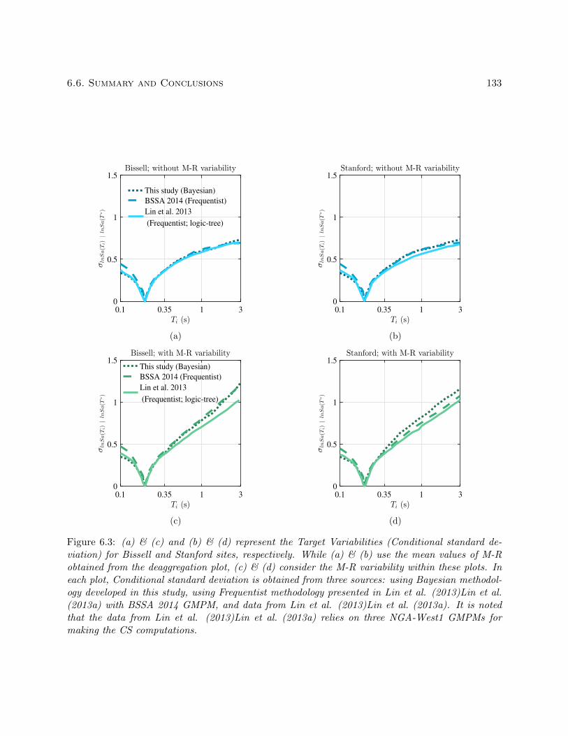
6.6. Summary and Conclusions 133
0.1 0.35 1 3
Ti (s)
0
0.5
1
1.5
σlnSa(T
i)|lnSa(T
∗)
Bissell; without M-R variability
This study (Bayesian)
BSSA 2014 (Frequentist)
Lin et al. 2013
(Frequentist; logic-tree)
(a)
0.1 0.35 1 3
Ti (s)
0
0.5
1
1.5
σlnSa(T
i)|lnSa(T
∗)
Stanford; without M-R variability
(b)
0.1 0.35 1 3
Ti (s)
0
0.5
1
1.5
σlnSa(T
i)|lnSa(T
∗)
Bissell; with M-R variability
This study (Bayesian)
BSSA 2014 (Frequentist)
Lin et al. 2013
(Frequentist; logic-tree)
(c)
0.1 0.35 1 3
Ti (s)
0
0.5
1
1.5
σlnSa(T
i)|lnSa(T
∗)
Stanford; with M-R variability
(d)
Figure 6.3: (a) & (c) and (b) & (d) represent the Target Variabilities (Conditional standard de-viation) for Bissell and Stanford sites, respectively. While (a) & (b) use the mean values of M-Robtained from the deaggregation plot, (c) & (d) consider the M-R variability within these plots. Ineach plot, Conditional standard deviation is obtained from three sources: using Bayesian methodol-ogy developed in this study, using Frequentist methodology presented in Lin et al. (2013)Lin et al.(2013a) with BSSA 2014 GMPM, and data from Lin et al. (2013)Lin et al. (2013a). It is notedthat the data from Lin et al. (2013)Lin et al. (2013a) relies on three NGA-West1 GMPMs formaking the CS computations.
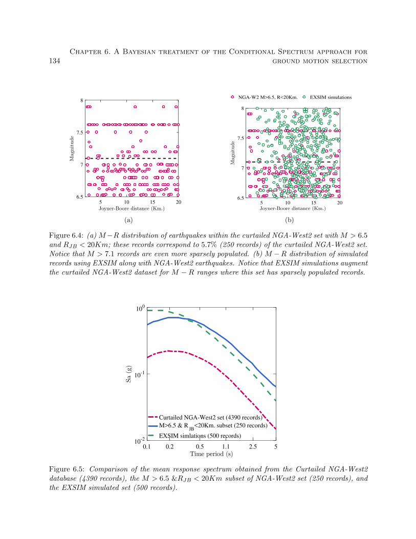
134Chapter 6. A Bayesian treatment of the Conditional Spectrum approach for
ground motion selection
5 10 15 20
Joyner-Boore distance (Km.)
6.5
7
7.5
8
Magnitude
(a)
5 10 15 20
Joyner-Boore distance (Km.)
6.5
7
7.5
8
Mag
nitude
NGA-W2 M>6.5, R<20Km. EXSIM simulations
(b)
Figure 6.4: (a) M−R distribution of earthquakes within the curtailed NGA-West2 set with M > 6.5and RJB < 20Km; these records correspond to 5.7% (250 records) of the curtailed NGA-West2 set.Notice that M > 7.1 records are even more sparsely populated. (b) M −R distribution of simulatedrecords using EXSIM along with NGA-West2 earthquakes. Notice that EXSIM simulations augmentthe curtailed NGA-West2 dataset for M −R ranges where this set has sparsely populated records.
0.1 0.2 0.5 1.1 2.5 5
Time period (s)
10-2
10-1
100
Sa(g)
Curtailed NGA-West2 set (4390 records)
M>6.5 & RJB
<20Km. subset (250 records)
EXSIM simlations (500 records)
Figure 6.5: Comparison of the mean response spectrum obtained from the Curtailed NGA-West2database (4390 records), the M > 6.5 &RJB < 20Km subset of NGA-West2 set (250 records), andthe EXSIM simulated set (500 records).

6.6. Summary and Conclusions 135
0.1 0.2 0.5 1.1 2.5 5
-4
-2
0
2
Value
Fault term
Likelihoods
Priors
Posteriors
(a)
0.1 0.2 0.5 1.1 2.5 5
0
1
2
3
M< 6.5 term 1
(b)
0.1 0.2 0.5 1.1 2.5 5
-1
-0.5
0
0.5
1
M< 6.5 term 2
(c)
0.1 0.2 0.5 1.1 2.5 5
Time period (s)
-2
-1
0
1
2
Value
M> 6.5 term
(d)
0.1 0.2 0.5 1.1 2.5 5
Time period (s)
-2
-1
0
1
lnR term
(e)
0.1 0.2 0.5 1.1 2.5 5
Time period (s)
-1
-0.5
0
0.5
1
M*lnR term
(f)
0.1 0.2 0.5 1.1 2.5 5
Time period (s)
-0.1
-0.05
0
0.05
0.1
Value
R term
(g)
0.1 0.2 0.5 1.1 2.5 5
Time period (s)
-1
-0.8
-0.6
-0.4
-0.2
Value
Vs30 term
(h)
Figure 6.6: Mean coefficient values across the spectral periods. Whereas the likelihoods and thepriors in this figure correspond to coefficient values inferred from the curtailed NGA-West2 and theEXSIM simulated sets, respectively, posteriors correspond to values obtained by combining thesetwo sets using Bayes rule.
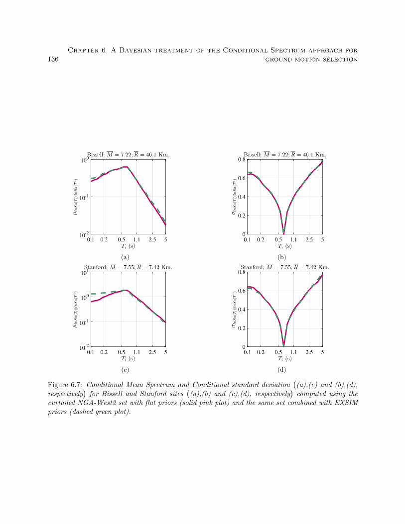
136Chapter 6. A Bayesian treatment of the Conditional Spectrum approach for
ground motion selection
0.1 0.2 0.5 1.1 2.5 5
Ti (s)
10-2
10-1
100
µlnSa(T
i)|lnSa(T
∗)
Bissell; M = 7.22;R = 46.1 Km.
(a)
0.1 0.2 0.5 1.1 2.5 5
Ti (s)
0
0.2
0.4
0.6
0.8
σlnSa(T
i)|lnSa(T
∗)
Bissell; M = 7.22;R = 46.1 Km.
(b)
0.1 0.2 0.5 1.1 2.5 5
Ti (s)
10-2
10-1
100
101
µlnSa(T
i)|lnSa(T
∗)
Stanford; M = 7.55;R = 7.42 Km.
(c)
0.1 0.2 0.5 1.1 2.5 5
Ti (s)
0
0.2
0.4
0.6
0.8
σlnSa(T
i)|lnSa(T
∗)
Stanford; M = 7.55;R = 7.42 Km.
(d)
Figure 6.7: Conditional Mean Spectrum and Conditional standard deviation((a),(c) and (b),(d),
respectively)
for Bissell and Stanford sites((a),(b) and (c),(d), respectively
)computed using the
curtailed NGA-West2 set with flat priors (solid pink plot) and the same set combined with EXSIMpriors (dashed green plot).
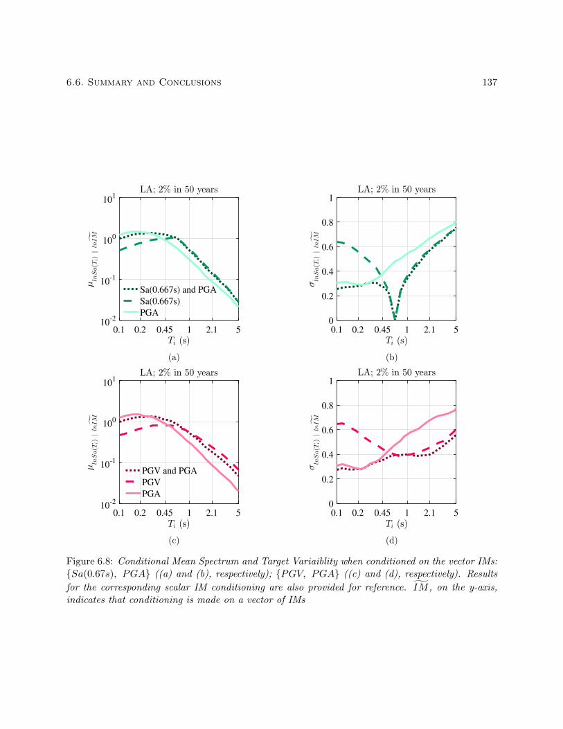
6.6. Summary and Conclusions 137
0.1 0.2 0.45 1 2.1 5
Ti (s)
10-2
10-1
100
101
µlnSa(T
i)|lnIM
LA; 2% in 50 years
Sa(0.667s) and PGA
Sa(0.667s)
PGA
(a)
0.1 0.2 0.45 1 2.1 5
Ti (s)
0
0.2
0.4
0.6
0.8
1
σlnSa(T
i)|lnIM
LA; 2% in 50 years
(b)
0.1 0.2 0.45 1 2.1 5
Ti (s)
10-2
10-1
100
101
µlnSa(T
i)|lnIM
LA; 2% in 50 years
PGV and PGA
PGV
PGA
(c)
0.1 0.2 0.45 1 2.1 5
Ti (s)
0
0.2
0.4
0.6
0.8
1
σlnSa(T
i)|lnIM
LA; 2% in 50 years
(d)
Figure 6.8: Conditional Mean Spectrum and Target Variaiblity when conditioned on the vector IMs:Sa(0.67s), PGA ((a) and (b), respectively); PGV, PGA ((c) and (d), respectively). Results
for the corresponding scalar IM conditioning are also provided for reference. IM , on the y-axis,indicates that conditioning is made on a vector of IMs
Chapter 7
Conclusions and future
recommendations
Intensity Measure (IM) and ground motion selection in Performance-Based Earthquake Engineering
(PBEE) govern the decision hazard which serves as an interface between performance specification
and structural design. This thesis has proposed methods for improved IM and ground motion
selection through the objectives listed in section 1.5. In this chapter, conclusions and future recom-
mendations concerning these contributions are discussed in addition to discussing the limitations of
the contributions made in this thesis. Moreover, comments are made on the application of Bayesian
methods in achieving the objectives proposed in Chapter 1 of this dissertation.
7.1 Summary
7.1.1 A unified metric for Intensity Measure quality assessment
IM selection is routinely performed for seismic risk assessment of structures using criteria such
as efficiency (or precision in predicting the structural response) and sufficiency (or accuracy in
representing the earthquake process and ground motion). An IM that is not efficient and sufficient
may lead to a biased estimate of the seismic demand hazard and, by extension, the loss hazard.
However, methods for selecting an appropriate IM, given a structure and a site, as a whole have been
qualitative and have had multiple criteria. This has caused impediments not only to IM selection
given a suite of alternatives, but also to the improvement of the state-of-the-art in PBEE by further
understanding the role IM plays in relating efficiently and sufficiently to different Engineering
Demand Parameters (EDP). Thus, a unified metric that gauges an IM’s quality against the different
138
7.1. Summary 139
criterion would be useful.
While efficiency assessment of an IM is performed quantitatively through the standard devi-
ation metric, sufficiency assessment has been subjective through the use of p-values and has had
multiple criteria owing to the different seismological parameters from which IM sufficiency needs to
be evaluated. To remedy this issue, a quantitative sufficiency metric, termed the Total Information
Gain (TIG), from all the considered seismological parameters is first proposed. This is achieved by
employing Bayes rule and principles from information theory. The TIG metric is then related to
the standard deviation metric to develop a unified metric for IM quality assessment.
The following specific contributions/observations have been made in relation to developing the
unified metric for quality IM assessment:
• The seismic demand fragility functions(P (EDP > y|IM)
)are found to be sensitive to the
inclusion of seismological parameters in their computation. And the degree of this sensitivity
(or insufficiency) is found to depend on the choice of the IM. However, directly gauging the
divergences between fragility functions obtained with and without considering the seismolog-
ical parameters in the EDP-IM relationship is found to lead to a biased assessment of IM
sufficiency; this bias is attributed to an IM’s efficiency.
• To remedy the above problem, divergence between the conditional density distributions of
an IM (f(IM |EDP > y); computed through Bayes rule) obtained with and without consid-
ering a seismological parameter is assessed thorough the Information Gain (IG) metric1. A
probability density function, unlike the fragility function which is a Cumulative Distribution
Function, gives a thorough representation of the influence of a seismological parameter in the
EDP-IM relationship. Owing to the positivity of the IG, sufficiency of an IM from multiple
seismological parameters is assessed by adding the individual IGs to result in the TIG metric.
This TIG metric is treated as a quantitative representation of IM sufficiency.
• Sufficiency of an IM, as assessed through the TIG metric, is found to depend on the ground
motion set selected for seismic response analyses. This dependence is attributed to the asser-
tion that different ground motion sets differ in terms of seismological parameters distribution
1Information Gain metric is also termed as Kullback-Liebler divergence
140 Chapter 7. Conclusions and future recommendations
and Fourier frequency spectrum distribution which in turn affects the EDP-IM-seismological
parameter relationship. However, for the adopted steel moment frame model, irrespective of
the ground motion record set adopted, the same IM for a particular record set is found to
be generally most sufficient across the EDPs Roof Drift (RD), Inter-Story Drift Ratio (IDR)
and Joint Rotation (JR). This is because, RD and IDR are directly related to the structures
global drift, and JR significantly influences the structures global drift during an earthquake.
• The TIG metric is found to have a weak positive correlation with the standard deviation
metric on a log-log scale. This lends support to the assertion that an IM’s sufficiency and
efficiency are weakly related and hence, the existence of these two criterion for IM selection is
obligatory. Further, these metrics were also found to follow a bivariate Normal distribution
on a log-log scale, and this conclusion was utilized to develop the unified metric for IM quality
assessment. The unified metric is formulated by measuring how different an IM is from the
“perfect” IM2.
7.1.2 A pre-configured solution to vector seismic hazard analysis
Vector Probabilistic Seismic Hazard Analysis (PSHA), which studies the frequency of exceedence
of intensity levels concerning multiple seismic IMs, has important applications in PBEE. There has
been a proliferation in the use of vector IMs for computing the seismic demand fragilities. This is
due to a realization that multiple IMs contribute toward structural response during an earthquake,
and an IM (mostly Sa(T1)) may not always singularly correlate well with the EDP across different
structural types and configurations. In such cases, a vector of IMs is needed to accurately compute
the demand hazard, and the decision hazard, by integrating the vector IM demand fragility with
the vector seismic hazard. Vector PSHA is then also needed to identify the intensity levels of the
vector of IMs and the dominating earthquake parameters given a design level earthquake in order
to select appropriate ground motions for seismic response analyses.
Despite these key applications of vector PSHA, accurately computing the vector seismic hazard,
while being consistent with modern standards of seismic hazard analysis, is still challenging. A novel
2The “perfect” IM is absolutely sufficient and efficient, as the TIG and the standard deviation metrics for thisIM are both zeros.

7.1. Summary 141
approximation to vector PSHA using outputs from existing PSHA programs is thus proposed.
This proposal is made by first establishing a unique understanding of PSHA theory through the
formalization of three properties of seismic hazard deaggregation plots. Then, statistical tools such
as Copula functions are used to propose a pre-configured solution to vector PSHA that can be
applied irrespective of the site or the vector of IMs selected.
The following specific contributions/observations have been made in relation to developing the
pre-configured solution to vector PSHA:
• The first two properties of deaggregation plots (i.e., monotonically decreasing nature with
IM level and invariance to the choice of the IM for a low IM level) are independent of each
other and are considered to be basic. These properties result from the mathematics of PSHA.
However, these properties are also associated with corresponding physical interpretations: (i)
the first property states that, with the earthquake source parameters fixed, the frequency of
exceedence of stronger ground motions always recedes; (ii) the second property states that
every earthquake, however small, should result in some ground motion 3.
• The third property of deaggregation plots (i.e., each deaggregation bin is part of a CCDF4
of the IM) can be derived as a corollary to the first two, by using Bayes rule. The physical
interpretation of the third property is similar to the first one, with the exception that frequen-
cies of exceedence (of IM levels) are now expressed as probabilities of exceedence. This third
property, interestingly, allows the expression of scalar hazard analysis results in an alternative
manner.
• The idea behind the novel approximation towards vector PSHA is to extend the alterna-
tive expression of scalar hazard analysis computations, as a result of the third property of
deaggregation plots, to a vector of IMs. In this regard, multivariate statistical tools such as
Copula functions and correlation coefficients between the vector of IMs considered are used.
This novel approximation to vector PSHA, then, not only uses the basic outputs from most
PSHA programs available, but also is mathematically consistent with the current standards
3The validity of these properties to duration related IMs, such as 5-95% significant duration, needs furtherexploration.
4CCDF: Complementary Cumulative Distribution Function
142 Chapter 7. Conclusions and future recommendations
of PSHA (i.e., logic tree and fault specific parameters of the multiple sources analyzed).
7.1.3 A Bayesian modification to the Conditional Spectrum approach for ground
motion selection
Appropriate ground motion selection is crucial for accurate assessment of structural response uncer-
tainties. A general and flexible ground motion selection target, employing principles from Bayesian
analysis, is proposed to accommodate the varied consensus on the “right” input motions. The de-
velopment of this target takes motivation from the Conditional Spectrum (CS) which constitutes
the Conditional Mean Spectrum (CMS) and the Target Variability (TV). Different features and
capabilities of this selection target, in terms of being general and flexible, were demonstrated by
applying it to example sites located in Los Angeles and Seattle. The following specific contribution-
s/observations are made in relation to developing the general and flexible ground motion selection
target:
• The CS is cast into a Bayesian framework to improve its adaptability to ground motion
selection preferences. An example of this is when multiple values of the rupture parameters
[such as Magnitude (M) and Distance (R)] can result in the same ground motion, and the
analyst is interested to consider this variability in M and R, given an IM value, for ground
motion selection. It was observed that irrespective of the site considered, low IM values
resulted in high M-R variability, as obtained from the deaggregation plots, influencing the
TV around the CMS. On the other hand, at sites such as Seattle, it was observed that
accounting for M-R variability was necessary even for large ground motion levels (i.e., ground
motions associated with high return periods) to result in an accurate representation of the CS.
Large M-R variability within the deaggregation plots is a result of multiple seismic sources
playing a dominant role in controlling the ground motion at a site.
• Additional information about the earthquake process can be incorporated into CS calculations
by adjusting the prior distributions in the Bayesian CS approach. This information depends
on the analyst, and can range from using a specific set of ground motions that result from
a particular type of earthquake rupture to the use of high consequence ground motions only.
7.2. Comments on the application of Bayesian methods in this dissertation 143
As an example, the use of large M-small R motions, by augmenting the NGA-West2 database
with priors from a ground motion simulation software, resulted in inflation of the CMS and
the TV amplitudes at low spectral periods. This inflation is attributed to sensitivity of low
spectral periods to earthquake characteristics more so than high periods.
The Bayesian CS is an improvement over the original CS (Baker, 2011) since it permits: (1)
considering M-R variability in calculations, thus improving the accuracy of the CS; (2) use of
vector-valued IMs as conditioning IMs (including non-spectral IMs), thereby leading to a ground
motion selection target which correctly represents the sensitivity of a structure to multiple IMs; (3)
incorporation of additional ground motion sets (through priors) which are not a part of the ground
motion database but might be critical for the specific project. Improvement (1) was considered
independently by Lin et al. (2013a), and improvement (2) was considered only for spectral/non-
spectral scalar conditioning IMs by Bradley (2010b). However, improvement (3) may only be
offered through the Bayesian conception of the CS since priors are permitted. More importantly,
the ability of the Bayesian CS to offer all the above improvements to the CS at the same time, and
not individually, is noteworthy.
7.2 Comments on the application of Bayesian methods in this
dissertation
The change of perspective, and the mechanism to incorporate additional information provided by
Bayesian methods were utilized in the following ways in this thesis.
The change of perspective provided by Bayes rule is what enabled the development of a metric
for IM sufficiency discussed previously. While developing the TIG metric to quantify IM sufficiency,
care needed to be taken to dampen the effects of IM efficiency; as it would be trivial to propose a
metric that is heavily influenced by efficiency. This is the reason why a transformation was made
from the EDP |IM space to the IM |EDP space using Bayes rule. Not only does this transformation
allow for sufficiency assessment independently5 of the efficiency, but it is also consistent with the
notion that sufficiency is a property of the IM, under the backdrop of an EDP.
5To say absolute independence would be an exaggeration, so marginal independence is an apt choice of words.
144 Chapter 7. Conclusions and future recommendations
A Bayesian transformation has also played a key role toward developing the simplified method
for vector PSHA. A simplified vector PSHA that considers multiple branches in a logic-tree and
multiple seismic sources near a site, while only having to use the scalar PSHA products6 from PSHA
software might, at first, may seem daunting. However, these products contain all the information
that is necessary to perform a vector PSHA; it is only that they need to be expressed in a way
that enables us to leverage this information. Thus, deaggregation matrices(P (M,R|IM > x)
)are transformed using Bayes rule to derive the aggregated conditional probability of IM exceedence(PA(IM > x|M,R)
). This PA(IM > x|M,R), which constitutes the third property of deaggre-
gation matrices, provides a pathway toward vector hazard analysis along which Copula functions
serve as tools for a multivariate analysis.
The application of a Bayesian methods toward proposing a Bayesian modification to the CS is
more obvious as compared with the other two applications previously discussed. Bayes rule, for the
present case, connects the following two interpretations concerning ground motion prediction which
is key to the development of the CS: (i) given a set of predictor variables (i.e., magnitude, distance,
. . . ) and a combination of such variables dictated by a functional form and the respective regression
coefficients, intensity of ground motions can be inferred; (ii) given a set of predictor variables that
cause ground motions and the ground motions themselves, a set of regression coefficients dictated
by a functional form can be inferred. These statements are summarized in equation (6.8) of Chapter
6.
7.3 Critique of the present work
In meeting the objectives laid out in section 1.5, several methods spanning three chapters were
proposed. The limitations of these contributions are now discussed.
7.3.1 A unified metric for intensity measure selection in PBEE
With the aim of proposing a unified metric to gauge an IM’s quality, a quantitative metric for
sufficiency from multiple earthquake parameters, the TIG metric, is first proposed. TIG is applied
6The hazard curves and the deaggregation matrices.
7.3. Critique of the present work 145
to a steel moment frame building considering 192 combinations of IMs, EDPs, and ground motion
record sets. For 177 of these 192 combinations, it is observed that TIG quantitatively represented
visual differences in the demand hazard curves when earthquake parameters were included in their
computation. There is a need to understand why the TIG was unable to properly gauge sufficiency
concerning the other 15 combinations. Moreover, the TIG needs to be applied to other building
types and sites to support further validation.
The TIG metric is proposed to be suitable with a cloud-analysis procedure that quantifies
the uncertainty in EDP given an IM. Furthermore, sufficiency of only scalar IMs were of interest.
Given the other alternative methods for relating EDP and IM, such as multiple stripe analysis
and incremental dynamic analysis, and the increasing commonality of preference for vector IMs in
PBEE, there is a need to expand the scope of the TIG metric to be suitable for these cases.
The unified metric for assessing the IM quality is derived upon first observing that the TIG
(sufficiency) and the standard deviation (efficiency) metrics are bi-variate Normally distributed
in a log-log space, and then by applying a Mahalanobis transformation (or a standard normal
transformation; Vidakovic 2011) to these metrics. It is noted that this formulation of the unified
metric depends on the bi-variate Normality observation of the sufficiency and the efficiency metrics.
While this observation holds for the steel moment frame building studied here, its validity for other
building types needs to be tested.
7.3.2 A pre-configured solution for vector probabilistic seismic hazard analysis
The simplified method for vector PSHA was validated for a hypothetical site surrounded by two fault
sources where PSHA computations are made using a logic-tree that is composed of eight branches.
Further validation of this simplified method is necessary concerning real sites where the seismic
activity can be more complex. Such a validation for realistic cases, however, is difficult because
exact PSHA computations, even for a single IM, require a lot of specific information concerning the
fault properties, logic-tree branches, statistics of seismic activity, and so on. And this information
is neither compiled in public databases nor retrievable from existing PSHA software. Despite this
limitation, a method for validating the simplified approach for vector PSHA for real sites needs to
be envisaged.
146 Chapter 7. Conclusions and future recommendations
Furthermore, such a validation will provide a foundation for investigating the influence of the
choice of Copula functions in the proposed simplified PSHA approach. A Gaussian Copula produced
accurate vector PSHA results for the above-mentioned hypothetical site, although, it was noted
earlier that this Copula’s validity for other sites needs to be further tested. More generally speaking,
a formal investigation assessing the suitability of various Copula types concerning different sites
and seismicity conditions needs to be undertaken.
7.3.3 A Bayesian implementation of the Conditional Spectrum approach for
ground motion selection
A Bayesian modification to the CS is proposed to provide flexibility and adaptability toward ground
motion selection preferences, as previously discussed. A limitation of this modification is the
restriction toward a prescribed functional form for ground motion prediction. Should the analyst
desire to use an alternative functional form, the source code for the Bayesian algorithm needs to be
modified, thus, placing a constraint on adaptability. To alleviate this limitation, one solution is to
program the source code to be consistent with the alternative ground motion prediction functional
forms generally utilized in practice.
Another generalized, but mathematically complex, solution is to is to develop a likelihood-free
Bayesian formulation for the CS. Such a formulation does not rely on any ground motion prediction
functional form, and the algorithm implicitly chooses the best functional form depending on the
ground motion and predictor variable data supplied by the analyst. This approach is also a step
forward in that it is similar to the modern (machine) learning approaches, but with the additional
advantages a Bayesian philosophy offers.
7.4 Looking forward: an integrated approach for intensity mea-
sure and ground motion selection in PBEE
Two methods that enable a more informed IM and ground motion selection for PBEE analysis were
proposed under a Bayesian lens. Although these methods, by themselves, are independently appli-

7.4. Looking forward: an integrated approach for intensity measure and groundmotion selection in PBEE 147
cable to IM and ground motion selection, respectively, the fact that they both are Bayesian might
allow for their integration. Such an integrated approach has the potential to resolve the issue of the
sensitivity of loss hazard to IM and ground motion selection, but it also will be computationally
tractable. In this regard, it is expected that the unified metric for rating alternative IMs and the
general and flexible ground motion selection tool proposed in this dissertation would play a key
role.
The integrated, Bayesian approach can be achieved by employing a statistical learning algo-
rithm termed Naıve Bayes Classifier. This algorithm takes into account “all possible” IM and
ground motion preferences and their corresponding ratings through the unified metric. Each time
a new IM and ground motion preference is fed into the algorithm, the decision-hazard is updated in
light of this new information, owing to the adoption of a Bayesian philosophy. The decision-hazard
is said to be precise when a new preference fed into the framework leads to a negligible change.
Furthermore, the final decision-hazard is said to be accurate when it is consistent with results
obtained from Monte-Carlo simulations.
Broadly speaking, the integrated approach for IM and ground motion selection has the potential
to improve the practicality and reliability of the PEER framework for PBEE. This in-turn leads
to a “right” sense of confidence on the designed building by giving neither an exaggerated- nor an
under-representation of the performance during and after an earthquake.

Appendices
148
Appendix A
Relation between IM efficiency and
its ground motion record
representation capacity
Jalayer et al. (2012) propose a definition of sufficiency which is different from the original sufficiency
criterion of Luco and Cornell (2007): a scalar IM should ideally be able to represent an entire
ground motion record in relation to an EDP . This is mathematically shown as:
f(EDP |xg) = f(EDP |IMi(xg)) (A.1)
where xg is the ground motion acceleration record.
Jalayer et al. (2012) propose a Relative Sufficiency Measure (RSM) which assesses the ground
motion representation capability of one IM in relation to another. In this appendix, we prove
that ground motion representation capability of IMs can be conveniently gaged by comparing the
standard deviations they render in predicting EDP . That is, standard deviation in lnEDP given
lnIM (this is usually termed IM efficiency) may be used directly to evaluate the ground motion
representation capacity of an IM without the need to calculate RSM.
By calculating the information gain when IM1 is used instead of IM2, the RSM evaluates how
well IM1 represents the ground motion record in comparison to IM2. A positive value of RSM
indicates IM1 is a better representative of the ground motion record and hence a better predictor
of response as compared to IM2 (Jalayer et al., 2012) . Negative and zero values of RSM can be
interpreted in a similar fashion. The definition of the RSM is given by (Jalayer et al., 2012):
149
150Appendix A. Relation between IM efficiency and its ground motion record
representation capacity
I(EDP |IM1|IM2) =
∫log2
p(EDP (xg)|IM1)
p(EDP (xg)|IM2)p(xg) dxg (A.2)
where I(EDP |IM1|IM2) represents information gain when IM1 is used instead of IM2, p(EDP (xg)|IMi)
represents the probability density of response (EDP ) given a ground motion record (xg) condi-
tioned upon a particular IM , IMi. This probability density is evaluated by assuming that the
response given IM is log-normally distributed (Ebrahimian et al., 2015; Tubaldi et al., 2016).
p(xg) represents the probability density of observing a particular earthquake ground motion and is
evaluated through stochastic ground motion simulations (Atkinson and Silva, 2000; Jalayer et al.,
2012). Jalayer et al. (2012) also propose an approximate RSM by assuming that all the ground
motion records are equally likely to occur. Unlike the exact RSM, the approximate RSM does not
require stochastic ground motion simulations and is readily applicable. The approximate RSM is
given by (Ebrahimian et al., 2015):
I(EDP |IM1|IM2) =1
Nr
Nr∑n=1
log2p(EDP (xg)|IM1)
p(EDP (xg)|IM2)(A.3)
where Nr is the number of earthquake records in the suite. It is noted from equation (A.3) that
the approximate RSM does not consider site specific information such as a seismic hazard curve
or hazard deaggregation.
When EDP and IM are transformed into a logarithmic space and it is assumed that p(.) in
equation (A.3) is calculated using a normal distribution, the computed RSM value does not change
(i.e., if random variable X is log-normally distributed then the random variable lnX is normally
distributed, Benjamin and Cornell 2014). The transformation is shown in equation (A.4) and can
be further simplified as shown in equation (A.5) using a property of logarithms and linearity of the
summation operator.
I(EDP |IM1|IM2) =1
Nr
Nr∑n=1
log2p(lnEDP (xg)| ln IM1)
p(lnEDP (xg)| ln IM2)(A.4)
151
I(EDP |IM1|IM2) =1
Nr
Nr∑n=1
log2 p(lnEDP | ln IM1)−1
Nr
Nr∑n=1
log2 p(lnEDP | ln IM2) (A.5)
Now, ordinary linear regression can be performed either by minimizing the sum of squares of
errors or by maximizing the sum of log-likelihoods under the normal distribution assumption. This
equivalence between these two operations is shown as (Hoff, 2009):
argminθ
Nr∑n=1
(lnEDP − ln ¯EDP )2 ⇔ argmaxθ
Nr∑n=1
log2 p(lnEDP | ln IMi) (A.6)
where EDP and ¯EDP denote the observed and predicted responses respectively, IMi denotes ith
IM in the suite and θ is a vector of regression coefficients. The left-hand side of the equation
represents minimization of sum squares of errors between observed and predicted log responses.
The right-hand side represents maximization of log-likelihoods of observed log responses under
the normal distribution assumption. Within a suite of IMs and under a cloud-based approach,
an IM with the least standard deviation in structural response has the least sum of squares of
errors in predicted responses (note that this also has been termed efficiency). Then because of the
equivalence in equation (A.6), this particular IM also has the maximum sum of log-likelihoods.
This further implies that if in equation (A.5) IM1 is selected such that it has the least standard
deviation in response (EDP ) and IM2 is any other IM in the suite, then the approximate RSM
value is bound to have a positive value. Such a trend has also been observed by Minas et al. (2015).
This indicates that the approximate RSM is actually a measure for relative efficiencies of two IMs.
Furthermore, a consequence of this logic is that, because deriving the RSM uses equation (A.1)
(refer to Jalayer et al. 2012 for the derivation), it can be said that an IM which is most efficient
among a suite of alternative IMs is also a better representative of the ground motion records, which
is quite intuitive.
Appendix B
Vector seismic hazard and
deaggregation: additional results
In this appendix, two additional aspects of chapter 5 are explored: (1) application of the vector
hazard approach for a suite of three Intensity Measures (IMs); (2) comparison of bi-variate hazard
the results obtained using Gaussian and ‘t’ Copulas.
B.1 Vector hazard and deaggregation for the IMs Sa(1s), PGA,
and PGV in LA, CA
Vector hazard and deaggregation are computed considering the three IMs: PGA, PGV , and Sa(1s)
at the a site in LA, CA (see section 5.5). The Pearson correlation coefficients between PGA−Sa(1s)
and PGV −Sa(1s) pairs are assumed as 0.43 and 0.78, respectively (Bradley, 2011, 2012b). Figures
B.1a and B.1b provide vector hazard surfaces for the IM sets PGV, Sa(1s), PGA > 0.1g and
PGV, Sa(1s), PGA > 2g, respectively. Figure B.1c provides vector deaggregation corresponding
to the IM levels PGV > 150cm/s, Sa(1s) > 0.5g, PGA > 0.5g. By comparing Figure B.1a and
B.1b, it can be noticed that depending upon the PGA level considered, the vector hazard surface
between PGV and Sa(1s) significantly changes in terms of the Annual Frequency of Exceedance
(AFE). However, the vector deaggregation plot (Figure B.1c) conditioned on the three IM levels is
quite similar the one shown in Figure 5.10b.
152
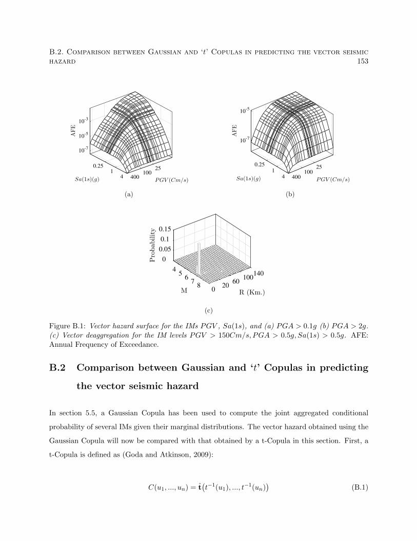
B.2. Comparison between Gaussian and ‘t’ Copulas in predicting the vector seismichazard 153
10-7
10-5A
FE
0.25
10-3
Sa(1s)(g)
25
PGV (Cm/s)
1 1004 400
(a)
10-7
0.25
AFE
Sa(1s)(g)
25
PGV (Cm/s)
1 100
10-5
4 400
(b)
0
0.05
4
0.1
Probab
ility 0.15
5 140
M
6 100
R (Km.)
7 60 8 20
0
(c)
Figure B.1: Vector hazard surface for the IMs PGV , Sa(1s), and (a) PGA > 0.1g (b) PGA > 2g.(c) Vector deaggregation for the IM levels PGV > 150Cm/s, PGA > 0.5g, Sa(1s) > 0.5g. AFE:Annual Frequency of Exceedance.
B.2 Comparison between Gaussian and ‘t’ Copulas in predicting
the vector seismic hazard
In section 5.5, a Gaussian Copula has been used to compute the joint aggregated conditional
probability of several IMs given their marginal distributions. The vector hazard obtained using the
Gaussian Copula will now be compared with that obtained by a t-Copula in this section. First, a
t-Copula is defined as (Goda and Atkinson, 2009):
C(u1, ..., un) = t(t−1(u1), ..., t
−1(un))
(B.1)

154 Appendix B. Vector seismic hazard and deaggregation: additional results
where t denotes a Multivariate t-distribution CDF with a correlation matrix and ν Degrees Of
Freedom (DOF); t−1 denotes an inverse t-distribution CDF with ν DOF. A ‘t’-Copula maybe
more effective in capturing the dependences between the IMs at the tails of the distribution(i.e.
between PA(IM1 < x1|Mj , Rj), ..., PA(IMn < xn|Mj , Rj))
than a Gaussian Copula. However, it is
interesting to note that a ‘t’-Copula with a large number of DOF—of the order 103—is equivalent
to a Gaussian Copula. Therefore, in order to explore the influence of using a ‘t’-Copula for a lower
number of DOF, we decided to fix this value to 15.
Figure B.2 provides a comparison between the vector hazards obtained using a Gaussian Copula
and a t-Copula. Four IM combinations are considered: PGV and PGA > 0.5g; PGV and PGA >
2g; PGA and PGV > 150Cm/s; PGA and PGV > 300Cm/s. It can be observed that at
moderate values of the conditioned IM (PGA and PGV in Figures B.2a and B.2b, respectively),
both Gaussian and ‘t’ Copulas produce similar results. However, at large values of the conditioned
IM (Figures B.2c and B.2d), the ‘t’-Copula tends to predict higher hazards relative to the Gaussian
Copula. As a t-Copula places more weight on the tails of a distribution (i.e. the joint aggregated
exceedance probabilities for high IM levels), we expect the results in Figure B.2 under this Copula
type to be influenced by its heavy-tailedness; however, a more thorough investigation should be
undertaken.
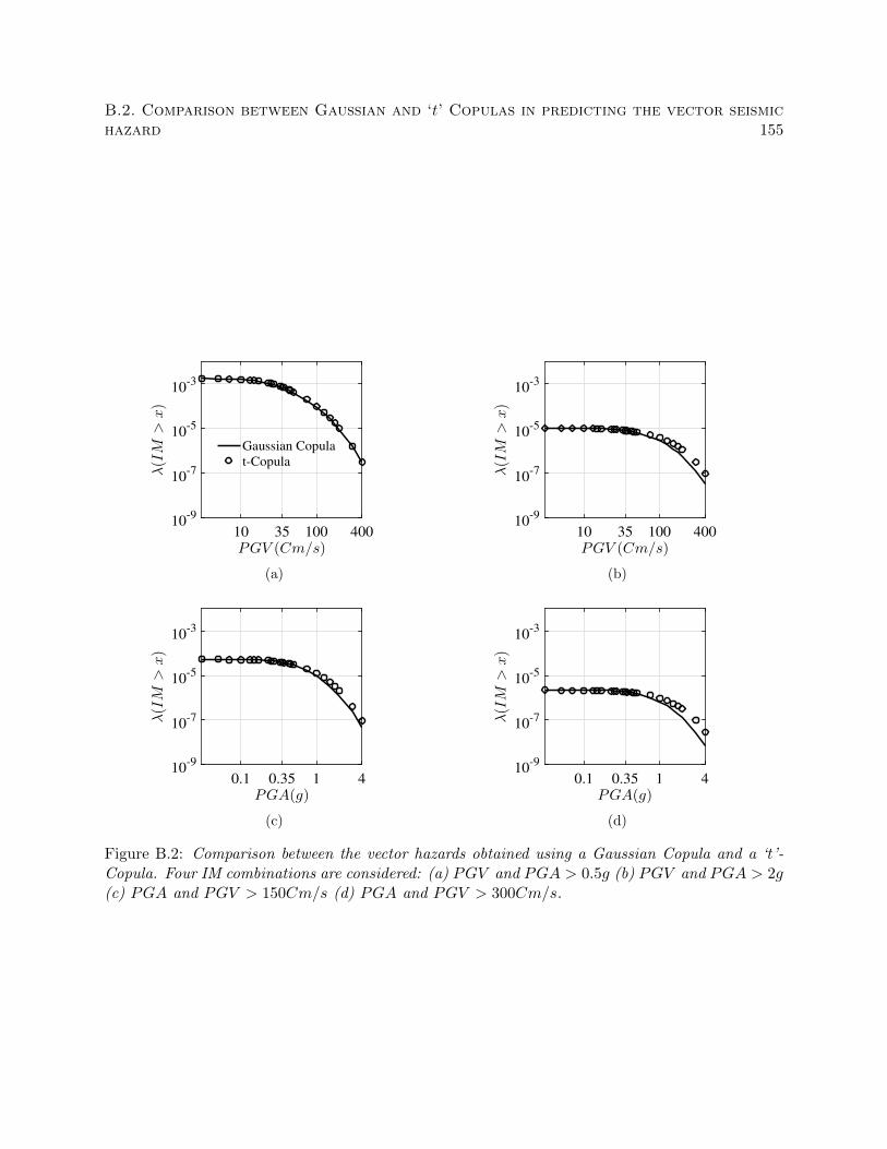
B.2. Comparison between Gaussian and ‘t’ Copulas in predicting the vector seismichazard 155
10 35 100 400PGV (Cm/s)
10-9
10-7
10-5
10-3
λ(IM
>x)
Gaussian Copula
t-Copula
(a)
10 35 100 400
PGV (Cm/s)
10-9
10-7
10-5
10-3
λ(IM
>x)
(b)
0.1 0.35 1 4
PGA(g)
10-9
10-7
10-5
10-3
λ(IM
>x)
(c)
0.1 0.35 1 4
PGA(g)
10-9
10-7
10-5
10-3
λ(IM
>x)
(d)
Figure B.2: Comparison between the vector hazards obtained using a Gaussian Copula and a ‘t’-Copula. Four IM combinations are considered: (a) PGV and PGA > 0.5g (b) PGV and PGA > 2g(c) PGA and PGV > 150Cm/s (d) PGA and PGV > 300Cm/s.
Appendix C
Posterior distributions of the
parameter matrices α and Σ for the
Gibbs sampling MCMC scheme
Deriving the posterior full conditional distributions of the parameters matrices α and Σ for the
Bayesian computations presented in chapter 6 forms a key aspect in the implementation of the Gibbs
sampling (Algorithm 4). In this appendix, closed-form equations for p(α|Y,X,Σ) and p(Σ|Y,X, α)
are presented.
C.1 Prior distributions for α and Σ
The parameter matrix α is first vectorized by stacking the elements in its columns. This is mathe-
matically represented as, αv = vec(α). Now, the prior distribution for αv is considered to follow a
Multivariate Normal distribution with mean vector αv0 and covariance matrix ∆:
p(αv) ∝ |∆|−1/2 exp−1
2
(αv − αv0
)T∆−1
(αv − αv0
)(C.1)
The prior distribution for Σ is considered to follow an inverse-Wishart distribution with scale
matrix Q and degrees of freedom ν:
p(Σ) ∝ |Σ|−ν/2 exp−1
2Tr(Σ−1Q
)(C.2)
156

C.2. Posterior distributions for α and Σ 157
where Tr(.) indicates the trace of a matrix.
C.2 Posterior distributions for α and Σ
Posterior distributions for α and Σ are derived utilizing the Bayes’ rule:
p(χ|Y,X) ∝ p(Y|χ,X) p(χ) (C.3)
where χ is a variable of interest, and Y and X are the matrices of observations and predictors,
respectively.
The posterior full conditional distribution for αv is a Multivariate Normal distribution and is
given by (Rowe, 2003):
p(αv|Y,X,Σ) ∝ exp−1
2
(αv − αv
)T (∆−1 + XTX⊗Σ−1
)(αv − αv
)(C.4)
and,
αv =[∆−1 + XTX⊗Σ−1
]−1 [∆−1αv0 +
(XTX⊗Σ−1
)vec[YTX
(XTX
)−1]](C.5)
In the above two equations, ⊗ represents a Hadamard product.
The posterior full conditional distribution for Σ is an inverse-Wishart distribution and is given
by (Rowe, 2003):
p(Σ|Y,X, α) ∝ |Σ|−(No+ν)/2 exp−1
2Tr(Σ−1
[(Y −XαT)T (Y −XαT) +Q
])(C.6)
Appendix D
Is the correlation structure between
seismic intensity measures rupture
dependent?
D.1 Introduction
Correlations between seismic Intensity Measures (IM) are generally assumed to be constant in
literature. Dependence of these correlations on the earthquake rupture (Magnitude (M), Distance
(R), fault-type, . . . ) has consequences to seismic hazard analysis and performance-based earthquake
engineering. Procedures for computing the seismic hazard for a vector of IMs, then, need to account
for this changing correlation with the rupture condition, leading to a revision of the computed return
periods (Dhulipala et al., 2018a). Moreover, ground motion selection tools such as the Conditional
Spectrum (Lin et al., 2013a), which rely on the correlations between IMs, also need to consider this
variable correlation structure. This, then, not only influences the matched ground motions, but
also the seismic response analyses outputs such as the demand fragility function and the demand
hazard curve. An investigation on the dependence of the IM correlation structure on the rupture
is hence crucial.
There are several studies in the literature that have investigated the dependence of IM corre-
lations on earthquake rupture. The Azarbakht et al. (2014) study, by partitioning the NGA-West2
database Ancheta et al. (2014) into subsets, found correlations between spectral IMs to depend on
both M and R. Baker and Bradley (2017), on the other hand, showed that correlations between
spectral as well as non-spectral IMs within the NGA-West2 set had no significant dependence on
158
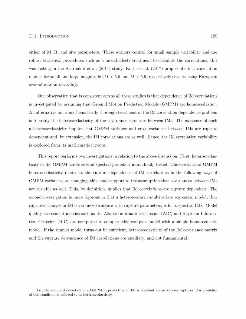
D.1. Introduction 159
either of M, R, and site parameters. These authors control for small sample variability and use
robust statistical procedures such as a mixed-effects treatment to calculate the correlations; this
was lacking in the Azarbakht et al. (2014) study. Kotha et al. (2017) propose distinct correlation
models for small and large magnitude (M < 5.5 and M > 5.5, respectively) events using European
ground motion recordings.
One observation that is consistent across all these studies is that dependence of IM correlations
is investigated by assuming that Ground Motion Prediction Models (GMPM) are homoscedastic1.
An alternative but a mathematically thorough treatment of the IM correlation dependence problem
is to verify the heteroscedasticity of the covariance structure between IMs. The existence of such
a heteroscedasticity implies that GMPM variance and cross-variances between IMs are rupture
dependent and, by extension, the IM correlations are as well. Hence, the IM correlation variability
is explored from its mathematical roots.
This report performs two investigations in relation to the above discussion. First, heteroscedas-
ticity of the GMPM across several spectral periods is individually tested. The existence of GMPM
heteroscedasticity relates to the rupture dependence of IM correlations in the following way: if
GMPM variances are changing, this lends support to the assumption that covariances between IMs
are variable as well. This, by definition, implies that IM correlations are rupture dependent. The
second investigation is more rigorous in that a heteroscedastic-multivariate regression model, that
captures changes in IM covariance structure with rupture parameters, is fit to spectral IMs. Model
quality assessment metrics such as the Akaike Information Criterion (AIC) and Bayesian Informa-
tion Criterion (BIC) are computed to compare this complex model with a simple homoscedastic
model. If the simpler model turns out be sufficient, heteroscedasticity of the IM covariance matrix
and the rupture dependence of IM correlations are auxiliary, and not fundamental.
1I.e., the standard deviation of a GMPM in predicting an IM is constant across various ruptures. An invalidityof this condition is referred to as heteroscedasticity.
160Appendix D. Is the correlation structure between seismic intensity measures
rupture dependent?
Table D.1: Bruesch-Pagan test for GMPM heteroscedasticity concerning spectral IMs. Null hy-pothesis: The GMPM is homoscedastic.
Spectral period (s) Bruesch-Pagan p-value Result at 0.05 significance level
0.1 5.90e-10 Accept null0.19 8.20e-05 Accept null0.3 0.063 Reject null0.42 2.10e-04 Accept null0.667 1.29e-08 Accept null0.9 1.10e-11 Accept null1.1 1.85e-14 Accept null1.3 2.20e-16 Accept null1.5 1.45e-14 Accept null1.7 9.55e-15 Accept null2 6.70e-16 Accept null
D.2 Statistical testing to investigate the heteroscedasticity in IM
prediction
A GMPM of the form resembling BSSA 2014 Boore et al. (2014) (see Dhulipala and Flint (2018))
is adopted to test for heteroscedasticity in IM prediction. Testing was performed for spectral IMs.
The Bruesch-Pagan test, which is commonly used in both research and practice, assumes that
heteroscedasticity is a function of all the independent variables used for IM prediction. This test is
performed by computing a p-value against the null hypothesis that the GMPM is homoscedastic.
If this p-value is greater than a significance level (say 0.05), the null hypothesis is rejected and
heteroscedasticity of the GMPM is advocated.
Table D.1 presents the results of the Bruesch-Pagan test across several spectral periods. Two
observations can be made from these results: (i) The Bruesch-Pagan test almost consistently accepts
the null hypothesis that the GMPM is homoscedastic; (ii) Studying the p-values, it is interesting
to note that evidence for heteroscedasticity marginally increases between 0.1s to 0.3s and then
starts receding for large spectral periods. In conclusion, non-existence of GMPM heteroscedasticity
concerning spectral IMs lends support to the assumption that covariances between these IM are
also unchanging with the rupture condition. This further implies that spectral IM correlations are
D.3. Multivariate Heteroscedastic GMPM 161
constant. However, a more rigorous investigation is performed in the next section.
D.3 A multivariate heteroscedastic GMPM for spectral intensity
measures
D.3.1 Model formulation
Let No be the number of observations and Nt be the number of spectral periods considered. A
multivariate heteroscedastic GMPM uses the following functional form for mean prediction:
Y = XαT + E (D.1)
where Y is a No ×Nt matrix of log observations, X is a No ×Np matrix of predictors where
Np is the number of model coefficients2, α is a Nt × Np matrix of regression coefficients, and E
is a No ×Nt matrix of residuals. Further, elements in E are correlated and are associated with a
covariance matrix Σ that is rupture dependent. The rupture dependence of the covariance matrix
is expressed by the following functional form Hoff and Niu (2012):
Σ = Ψ + βXXTβ (D.2)
where Ψ is the ‘baseline’ covariance matrix and β is a Nt×Np matrix of regression coefficients
to model heteroscedastic covariance. It is noted that both the mean and the covariance model use
the same prediction variables.
Fitting a multivariate heteroscedastic regression model requires inferring α, β, and Ψ given
ground motion data. A Bayesian Gibbs sampling based algorithm proposed by Hoff and Niu
(2012) is used to make this inference concerning the NGA-West2 database. Hoff and Niu (2012)
also provide an R package covreg Niu and Hoff (2013), and this was utilized for performing the
2The prediction variables are similar to the ones used in BSSA 2014 GMPM, with some modifications as outlinedin Dhulipala and Flint (2018)
162Appendix D. Is the correlation structure between seismic intensity measures
rupture dependent?
computations. The analysis results are subsequently discussed.
D.3.2 Results
The following eleven spectral periods were considered for analysis: 0.1, 0.19, 0.3, 0.42, 0.667, 0.9,
1.1, 1.3, 1.5, 1.7, and 2 seconds. The heteroscedastic covariance model estimates 253 coefficients
(99 each for the mean and the covariance models, and 55 for the ‘baseline’ covariance) from a
subset of 2494 ground motions in the NGA-West2 database. The homoscedastic model, on the
other hand, estimates 154 coefficients (99 each for the mean and the covariance models, and 55
for the ‘baseline’ covariance) from the same dataset. While fitting these models, it was found that
the variance inflation of the model coefficients is negligible across the spectral periods considered,
which further implies that bias due to multicollinearity is ignorable.
The variation of the standard deviations σ with the rupture condition is found to depend
upon the spectral period under consideration. Figure D.1a, for example, presents the σ variation
for three spectral periods (0.1, 0.667, and 2s) within the ground motion dataset, in addition to
the homoscedastic σ represented by vertical lines. It is noted that while σ for the 0.667s period
is less variable, the 0.1s period is seen exhibit a high variability; the 2s periods, however, falls
in between concerning σ variability. Across these three spectral periods, it is interesting to note
that their corresponding homoscedastic σs fall towards the right-side tails of the heteroscedastic σ
distributions. This suggests there might be some bias in the heteroscedastic model with respect to
the homoscedastic one.
Variability of the correlation coefficients for three combinations of spectral periods, (0.1, 0.667),
(0.1, 2), and (0.667, 2), is presented in Figures D.1b, D.1c, and D.1d, respectively. The correspond-
ing constant correlations obtained from the Baker and Jayaram (2008) model are also represented
as vertical lines. These figures suggest that correlations between spectral periods can be highly
variable; however, a physical justification of this variability is hard to conceive. Especially when
the number of ground motion recordings for a fixed set of rupture parameters are scanty. The con-
stant correlations are seen to fall near the center of the correlation distributions in Figures D.1c,
and D.1d. Although, this is not true in Figure D.1b.

D.3. Multivariate Heteroscedastic GMPM 163
D.3.3 Evaluation using AIC and BIC
AIC tests the relative suitability of alternative models. AIC for the ith is computed as:
AICi = 2ki − 2ln(Li) (D.3)
where ki and Li are the number of model parameters and likelihood of the ith model, respec-
tively. Whereas the AIC for the multivariate-heteroscedastic model was found to be 488.24 (AIC1),
the multivariate-homoscedastic model has an AIC of 291.81 (AIC0). Lesser the AIC, better the
model. A relative evaluation of the two models can be performed by further computing the Relative
Likelihood (RL):
RL = exp((AIC0 −AIC1)/2
)(D.4)
It was found that the RL for the multivariate-heteroscedastic model, with respect to the
multivariate-homoscedastic one, is 1.3e − 86. This suggests a strong evidence against using the
former.
BIC is similar to AIC, although it additionally accounts for sample size. A BIC is computed
using:
BICi = ln(No)ki − 2ln(Li) (D.5)
BIC for the multivariate -heteroscedastic and -homoscedastic models are found to be 1961.1
(BIC1) and 1187.7 (BIC0), respectively. Lesser the BIC, better the model. A high value of the
change in BIC between these two models (∆BIC = 773.4) suggests that the former model may not
provide any substantially new information that is physical.
Even this rigorous evaluation, by fitting a multivariate-heteroscedastic model to ground motion
data, seems to advise against the rupture dependence of IM correlations. However, this conclusion
may be specific to the IMs and the ground motion dataset considered here.
164Appendix D. Is the correlation structure between seismic intensity measures
rupture dependent?
D.4 Conclusions
Two investigations were conducted to verify the rupture dependence of correlations between spectral
IMs. These investigations are different from the previous studies in that change in correlations with
the rupture parameters was explored from the perspective of heteroscedasticity of the GMPM. Both
these investigations advise against heteroscedasticity, both in IM prediction and IM covariances.
This, by extension, implies that consideration of rupture dependence of the IM correlations within
the NGA-West2 database may be unnecessary.
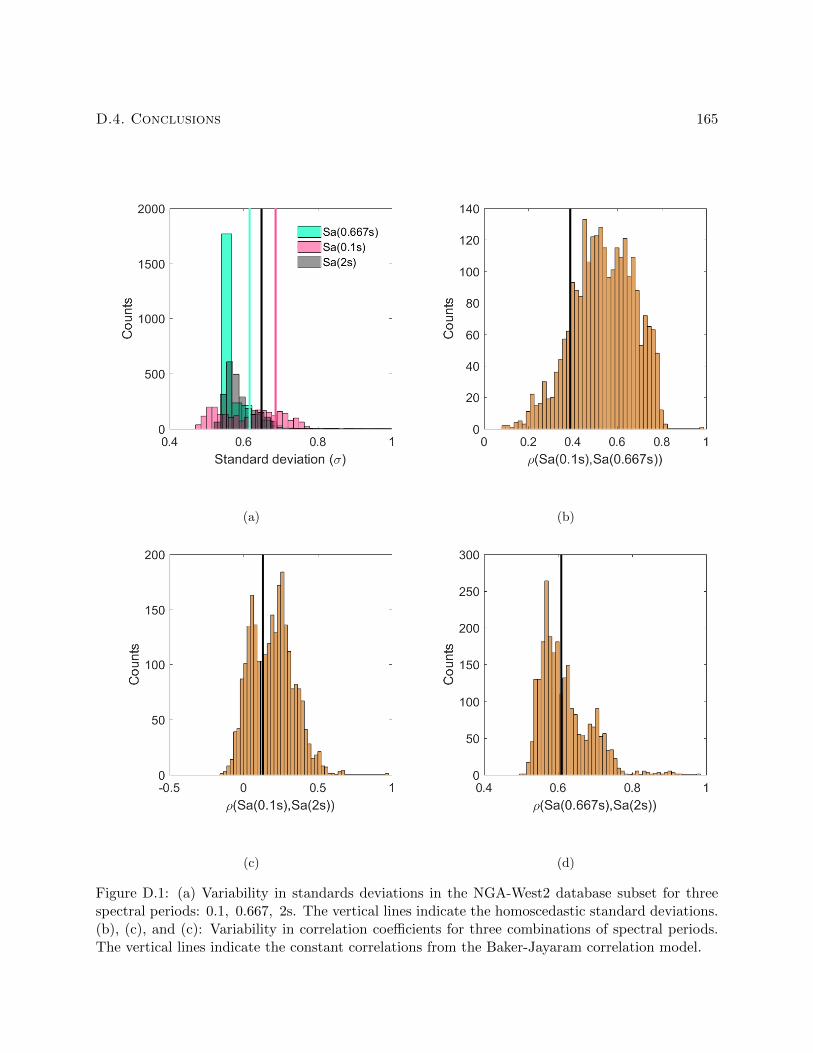
D.4. Conclusions 165
(a) (b)
(c) (d)
Figure D.1: (a) Variability in standards deviations in the NGA-West2 database subset for threespectral periods: 0.1, 0.667, 2s. The vertical lines indicate the homoscedastic standard deviations.(b), (c), and (c): Variability in correlation coefficients for three combinations of spectral periods.The vertical lines indicate the constant correlations from the Baker-Jayaram correlation model.
Bibliography
M. Aitkin. Modelling Variance Heterogeneity in Normal Regression Using GLIM. Journal of applied
statistics, 36(3):332–339, 1987.
A. Ali, N. A. Hayah, D. Kim, and S. G. Cho. Probabilistic seismic assessment of base-isolated NPPs
subjected to strong ground motions of tohoku earthquake. Nuclear Engineering and Technology,
46(5):699–706, 2014.
T. I. Allen and D. J. Wald. Topographic Slope as a Proxi for Seismic Site-Conditions (VS30) and
Amplification Around the Globe. Technical report, United States Geological Survey, Reston, VA,
2007.
B. P. Allmann and P. M. Shearer. Global variations of stress drop for moderate to large earthquakes.
Journal of Geophysical Research: Solid Earth, 114(1):1–22, 2009.
T. D. Ancheta, R. B. Darragh, J. P. Stewart, E. Seyhan, W. J. Silva, B. S. Chiou, K. E. Wooddell,
R. W. Graves, A. R. Kottke, D. M. Boore, T. Kishida, and J. L. Donahue. NGA-West2 database.
Earthquake Spectra, 30(3):989–1005, 2014.
D. Arroyo and M. Ordaz. Multivariate bayesian regression analysis applied to ground-motion
prediction equations, part 1: Theory and synthetic example. Bulletin of the Seismological Society
of America, 100(4):1551–1567, 2010a.
D. Arroyo and M. Ordaz. Multivariate bayesian regression analysis applied to ground-motion
prediction equations, part 2: Numerical example with actual data. Bulletin of the Seismological
Society of America, 100(4):1568–1577, 2010b.
ASCE. Minimum Design Loads in Buildings and Other Structures. American Society of Civil
Engineers, 2016.
ASCE7. Minimum Design Loads for Buildings and Other Structures. 2010.
166
BIBLIOGRAPHY 167
H. Aslani and E. Miranda. Probability-based seismic response analysis. Engineering Structures, 27
(8):1151–1163, 2005.
G. M. Atkinson and D. M. Boore. Earthquake ground-motion prediction equations for eastern
North America. Bulletin of the Seismological Society of America, 96(6):2181–2205, 2006.
G. M. Atkinson and W. Silva. Stochastic modeling of California ground motions. Bulletin of the
Seismological Society of America, 90(2):255–274, 2000.
B. O. Ay, M. J. Fox, and T. J. Sullivan. Practical Challenges Facing the Selection of Conditional
Spectrum-Compatible Accelerograms. Journal of Earthquake Engineering, 21(1):169–180, 2017.
A. Azarbakht, M. Mousavi, M. Nourizadeh, and M. Shahri. Dependence of correlations between
spectral accelerations at multiple periods on magnitude and distance. Earthquake Engineering
& Structural Dynamics, 43:1193–1204, 2014.
J. W. Baker. Probabilistic structural response assessment using vector-valued intensity measures.
Earthquake Engineering and Structural Dynamics, 36:1861–1883, 2007a.
J. W. Baker. Quantitative classification of near-fault ground motions using wavelet analysis. Bul-
letin of the Seismological Society of America, 97(5):1486–1501, 2007b.
J. W. Baker. An introduction to Probabilistic Seismic Hazard Analysis (PSHA). Technical report,
Stanford University, 2008.
J. W. Baker. Conditional Mean Spectrum: Tool for Ground-Motion Selection. Journal of Structural
Engineering, 137(March):322–331, 2011.
J. W. Baker and B. A. Bradley. Intensity measure correlations observed in the NGA-West2
database, and dependence of correlations on rupture and site parameters. Earthquake Spectra,
pages 1–17, 2016.
J. W. Baker and B. A. Bradley. Intensity Measure Correlations Observed in the NGA-West2
Database, and Dependence of Correlations on Rupture and Site Parameters. Earthquake Spectra,
33(1):145–156, 2017.
168 BIBLIOGRAPHY
J. W. Baker and C. A. Cornell. Vector-valued ground motion intensity measures for Probabilistic
Seismic Demand Analysis. PhD thesis, Stanford University, 2005.
J. W. Baker and C. A. Cornell. Spectral shape, epsilon and record selection. Earthquake Engineering
and Structural Dynamics, 35(9):1077–1095, 2006.
J. W. Baker and N. Jayaram. Correlation of spectral acceleration values from NGA ground motion
models. Earthquake Spectra, 24(1):299–317, 2008.
J. W. Baker and C. Lee. An Improved Algorithm for Selecting Ground Motions to Match a
Conditional Spectrum. Journal of Earthquake Engineering, 2017.
A. R. Barbosa. Simplified vector-valued probabilistic seismic hazard analysis and probabilistic seis-
mic demand analysis : application to the 13-story NEHRP reinforced concrete frame-wall building
design example. PhD thesis, University of California, San Diego, 2011.
P. Bazzurro and A. C. Cornell. Disaggregation of seismic hazard. Bulletin of the Seismological
Society of America, 89(2):501–520, 1999.
P. Bazzurro and A. C. Cornell. Vector-valued probabilistic seismic hazard analysis. In Seventh
U.S. National Conference on Earthquake Engineering, Boston, MA, 2002.
P. Bazzurro and J. Park. Vector-valued probabilistic seismic hazard analysis of correlated ground
motion parameters. In Applications of Statistics and Probability in Civil Engineering, pages
1596–1604, 2011.
P. Bazzurro, P. Tothong, and J. Park. Efficient approach to vector-valued probabilistic seismic
hazard analysis of multiple correlated ground-motion parameters. In International Conference
On Structural Safety And Reliability, Osaka, Japan, 2009.
J. R. Benjamin and A. C. Cornell. Probability, Statistics, and Decision for Civil Engineers. Courier
Corporation, 2014.
N. Bijelic, T. Lin, and G. G. Deierlein. Validation of the SCEC Broadband Platform simulations
for tall building risk assessments considering spectral shape and duration of the ground motion.
Earthquake Engineering & Structural Dynamics, pages 1–19, 2018.
BIBLIOGRAPHY 169
D. M. Boore and G. M. Atkinson. Ground-motion prediction equations for the average horizontal
component of PGA, PGV, and 5%-damped PSA at spectral periods between 0.01 s and 10.0 s.
Earthquake Spectra, 24(1):99–138, 2008.
D. M. Boore, J. P. Stewart, E. Seyhan, and G. M. Atkinson. NGA-West2 Equations for Predicting
Response Spectral Accelerations for Shallow Crustal Earthquakes. Earthquake Spectra, 30(3):
1057–1085, 2014.
Y. Bozorgnia and V. V. Bertero. Earthquake engineering: from engineering seismology to
Performance-Based Engineering. CRC press, 2004.
B. Bradley. The seismic demand hazard and importance of the conditioning intensity measure.
Earthquake Engineering & Structural Dynamics, 41(11):1417–1437, 2012a.
B. A. Bradley. A generalized conditional intensity measure approach and holistic ground-motion
selection. Earthquake Engineering & Structural Dynamics, 12(39):1321–1342, 2010a.
B. A. Bradley. A generalized conditional intensity measure approach and holistic ground-motion
selection. Earthquake Engineering & Structural Dynamics, (39):1321–1342, 2010b.
B. A. Bradley. Empirical correlation of PGA, spectral accelerations and spectrum intensities from
active shallow crustal earthquakes. Earthquake Engineering & Structural Dynamics, (40):1707–
1721, 2011.
B. A. Bradley. Empirical correlations between peak ground velocity and spectrum-based intensity
measures. Earthquake Spectra, 28(1):17–35, 2012b.
B. A. Bradley. A ground motion selection algorithm based on the generalized conditional intensity
measure approach. Soil Dynamics and Earthquake Engineering, 40:48–61, 2012c.
B. A. Bradley, M. Cubrinovski, R. P. Dhakal, and G. A. MacRae. Intensity measures for the seismic
response of pile foundations. Soil Dynamics and Earthquake Engineering, 29(6):1046–1058, 2009.
B. A. Bradley, L. S. Burks, and J. W. Baker. Ground motion selection for simulation-based seismic
hazard and structural reliability assessment. Earthquake Engineering & Structural Dynamics,
44:2321–2340, 2015.
170 BIBLIOGRAPHY
K. W. Campbell and Y. Bozorgnia. NGA ground motion model for the geometric mean horizontal
component of PGA, PGV, PGD and 5% damped linear elastic response spectra for periods
ranging from 0.01 to 10 s. Earthquake Spectra, 24(1):139–171, 2008.
B. Carlton and N. Abrahamson. Issues and approaches for implementing conditional mean spectra
in practice. Bulletin of the Seismological Society of America, 104(1):503–512, 2014.
E. Cepeda and D. Gamerman. Bayesian Modeling of Variance Heterogeneinty in normal regression
models. Brazilian Journal of Probability and Statistics, 14(2):207–221, 2001.
R. Chandramohan, J. W. Baker, and G. G. Deierlein. Impact of hazard-consistent ground motion
duration in structural collapse risk assessment. Earthquake Engineering & Structural Dynamics,
45:1357–1379, 2016.
T. M. Cover and T. A. Joy. Elements of Information Theory. 2012.
J. G. F. Crempien and R. J. Archuleta. UCSB Method for Simulation of Broadband Ground Motion
from Kinematic Earthquake Sources. Seismological Research Letters, 86(1):61–67, 2015. ISSN
0895-0695.
J. E. Daniell, B. Khazai, F. Wenzel, and A. Vervaeck. The CATDAT damaging earthquakes
database. Natural Hazards and Earth System Science, 11(8):2235–2251, 2011.
S. L. N. Dhulipala and M. M. Flint. A Bayesian Treatment of the Conditional Spectrum Approach
for Ground Motion Selection (in review). 2018.
S. L. N. Dhulipala, A. Rodriguez-Marek, and M. M. Flint. Computation of vector hazard using
salient features of seismic hazard deaggregation. Earthquake Spectra, 34(4):1–20, 2018a.
S. L. N. Dhulipala, A. Rodriguez-Marek, S. Ranganathan, and M. Flint. A site-consistent method to
quantify sufficiency of alternative IMs in relation to PSDA. Earthquake Engineering & Structural
Dynamics, 47(2):377–396, 2018b.
D. S. Dreger, G. C. Beroza, S. M. Day, C. A. Goulet, T. H. Jordan, P. A. Spudich, and J. P. Stewart.
Validation of the SCEC Broadband Platform V14.3 Simulation Methods Using Pseudospectral
Acceleration Data. Seismological Research Letters, 86(1):39–47, 2015. ISSN 0895-0695.
BIBLIOGRAPHY 171
L. Eads. Seismic Collapse Risk Assessment of Buildings: Effects of Intensity Measure Selection
and Computational Approach. PhD thesis, Stanford University, 2013.
L. Eads, E. Miranda, H. Krawinkler, and D. Lignos. An efficient method for estimating the collapse
risk of structures in seismic regions. Earthquake Engineering & Structural Dynamics, 42(1):25–41,
2013.
H. Ebrahimian, F. Jalayer, A. Lucchini, F. Mollaioli, and G. Manfredi. Preliminary ranking of
alternative scalar and vector intensity measures of ground shaking. Bulletin of Earthquake En-
gineering, 13(10):2805–2840, 2015.
FEMA P695. FEMA P-695: Quantification of building seismic performance factors. FEMA
P695. Technical Report June, 2009. URL http://www.fema.gov/media-library-data/
20130726-1716-25045-9655/fema_p695.pdf.
E. H. Field, T. H. Jordan, and A. C. Cornell. OpenSHA: A Developing Community - Modeling
Environment for Seismic Hazard Analysis. Seismological Research Letters, 74(4):406–419, 2003.
M. M. Flint, J. W. Baker, and S. L. Billington. A modular framework for performance-based
durability engineering: From exposure to impacts. Structural Safety, 50:78–93, 2014.
F. Freddi, J. E. Padgett, and A. Dall’Asta. Probabilistic seismic demand modeling of local level
response parameters of an RC frame. Bulletin of Earthquake Engineering, 15(1):1–23, 2016.
P. Giovenale, A. C. Cornell, and L. Esteva. Comparing the adequacy of alternative ground mo-
tion intensity measures for the estimation of structural responses. Earthquake Engineering and
Structural Dynamics, 33(8):951–979, 2004.
K. Goda and G. M. Atkinson. Interperiod dependence of ground-motion prediction equations: A
copula perspective. Bulletin of the Seismological Society of America, 99(2 A):922–927, 2009.
C. A. Goulet, C. B. Haselton, J. Mitrani-Reiser, J. L. Beck, G. G. Deierlein, K. A. Porter, and J. P.
Stewart. Evaluation of the seismic performance of a code-conforming reinforced-concrete frame
buildingfrom seismic hazard to collapse safety and economic losses. Earthquake Engineering &
Structural Dynamics, (36):1973–1997, 2007.

172 BIBLIOGRAPHY
C. A. Goulet, T. Kishida, T. D. Ancheta, C. H. Cramer, R. B. Darragh, W. J. Silva, Y. M. A.
Hashash, J. Harmon, J. P. Stewart, K. E. Wooddell, and R. R. Youngs. PEER NGA-East
database. Technical report, Pacific Earthquake Engineering Research, 2014.
C. A. Goulet, P. J. Maechling, S. Mazzoni, and F. Silva. SCEC BBP Study 17.3 Dataset.
DesignSafe-CI, 2018.
R. W. Graves and A. Pitarka. Refinements to the Graves and Pitarka (2010) Broadband Ground-
Motion Simulation Method. Seismological Research Letters, 86(1):75–80, 2015. ISSN 0895-0695.
R. W. Graves, T. H. Jordan, S. Callaghan, E. Deelman, E. Field, G. Juve, C. Kesselman, P. Maech-
ling, G. Mehta, K. Milner, D. Okaya, P. Small, and K. Vahi. CyberShake: A Physics-Based
Seismic Hazard Model for Southern California. Pure and Applied Geophysics, 168(3-4):367–381,
2011.
N. Gregor, N. A. Abrahamson, G. M. Atkinson, D. M. Boore, Y. Bozorgnia, K. W. Campbell,
B. S. J. Chiou, I. M. Idriss, R. Kamai, E. Seyhan, W. Silva, J. P. Stewart, and R. Youngs.
Comparison of NGA-West2 GMPEs. Earthquake Spectra, 30(3):1179–1197, 2014.
M. A. Hariri-Ardebili and V. E. Saouma. Probabilistic seismic demand model and optimal intensity
measure for concrete dams. Structural Safety, 59:67–85, 2016.
P. D. Hoff. A first course in Bayesian statistical analysis. Springer, Seattle, 1st edition, 2009.
P. D. Hoff and X. Niu. A covariance regression model. Statistica Sinica, 22:729–753, 2012.
L. F. Ibarra, R. A. Medina, and H. Krawinkler. Hysteretic models that incorporate strength
and stiffness deterioration. Earthquake Engineering and Structural Dynamics, 34(12):1489–1511,
2005.
F. Jalayer, J. L. Beck, and F. Zareian. Analyzing the Sufficiency of Alternative Scalar and Vector
Intensity Measures of Ground Shaking Based on Information Theory. Journal of Engineering
Mechanics, 138(3):307–316, 2012.
F. Jalayer, R. De Risi, and G. Manfredi. Bayesian Cloud Analysis: Efficient structural fragility
assessment using linear regression. Bulletin of Earthquake Engineering, 13(4):1183–1203, 2015.
BIBLIOGRAPHY 173
N. Jayaram and J. W. Baker. Statistical tests of the joint distribution of spectral acceleration
values. Bulletin of the Seismological Society of America, 98(5):2231–2243, 2008.
N. Jayaram, T. Lin, and J. W. Baker. A Computationally efficient ground-motion selection algo-
rithm for matching a target response spectrum mean and variance. Earthquake Spectra, 27(3):
797–815, 2011.
W. B. Joyner and D. M. Boore. Methods for regression analysis of strong-motion data. Bulletin of
the Seismological Society of America, 83(2):469–487, 1993.
O. Kale, J. E. Padgett, and A. Shafieezadeh. A ground motion prediction equation for novel peak
ground fractional order response intensity measures. Bulletin of Earthquake Engineering, 15(9):
3437–3461, 2017.
A. Kazantzi and D. Vamvatsikos. Intensity measure selection for vulnerability studies of building
classes. Earthquake Engineering & Structural Dynamics, 44(15):2677–2694, 2015.
T. Kishida. Conditional Mean Spectra Given a Vector of Spectral Accelerations at Multiple Periods.
Earthquake Spectra, 33(2), 2017.
M. Kohrangi, P. Bazzurro, and D. Vamvatsikos. Vector and Scalar IMs in Structural Response
Estimation, Part II: Building Demand. Earthquake Spectra, 32(3), 2016a.
M. Kohrangi, P. Bazzurro, and D. Vamvatsikos. Vector and Scalar IMs in Structural Response
Estimation: Part I Hazard Analysis. Earthquake Spectra, 32(3), 2016b.
M. Kohrangi, D. Vamvatsikos, and P. Bazzurro. Implications of intensity measure selection for
seismic loss assessment of 3-D buildings. Earthquake Spectra, 32(4):2167–2189, 2016c.
M. Kohrangi, D. Vamvatsikos, and P. Bazzurro. Site dependence and record selection schemes for
building fragility and regional loss assessment. Earthquake Engineering & Structural Dynamics,
2017.
M. Kohrangi, S. R. Kotha, and P. Bazzurro. Ground-motion models for average spectral acceleration
in a period range: Direct and indirect methods. Bulletin of Earthquake Engineering, 16(1):45–65,
2018.
174 BIBLIOGRAPHY
K. Konno and T. Ohmachi. Ground-motion characteristics estimated from spectral ratio between
horizontal and vertical components of microtremor. Bulletin of the Seismological Society of
America, 88(1):228–241, 1998.
M. E. Koopaee, R. P. Dhakal, and G. A. MacRae. Effect of ground motion selection methods on
seismic collapse fragility of RC frame buildings. Earthquake Engineering & Structural Dynamics,
46:1875–1892, 2017.
S. Kotha, D. Bindi, and F. Cotton. Site-corrected magnitude- and region- dependent correlations of
horizontal peak spectral amplitudes. Earthquake Spectra, 33(4):1415–1432, 2017. ISSN 87552930.
doi: 10.1193/091416EQS150M.
S. Kramer. Geotechnical earthquake engineering. Prentice Hall, New York, 1996.
H. Krawinkler. Advancing Performance-Based Earthquake Engineering, 1999. URL http://peer.
berkeley.edu/news/1999jan/advance.html.
S. N. Kwong and A. K. Chopra. A Generalized Conditional Mean Spectrum and its application for
intensity-based assessments of seismic demands. Earthquake Spectra, 33(1):1–28, 2016a.
S. N. Kwong and A. K. Chopra. Evaluation of the exact conditional spectrum and generalized
conditional intensity measure methods for ground motion selection. Earthquake Engineering &
Structural Dynamics, (45):757–777, 2016b.
T. Lin. Advancement of hazard-consistent ground motion selection methodology. PhD thesis, Stan-
ford University, 2012.
T. Lin, S. C. Harmsen, J. W. Baker, and N. Luco. Conditional spectrum computation incorporating
multiple causal earthquakes and ground-motion prediction models. Bulletin of the Seismological
Society of America, 103(2A):1103–1116, 2013a.
T. Lin, C. B. Haselton, and J. W. Baker. Conditional spectrum-based ground motion selection.
Part I: Hazard consistency for risk-based assessments. Earthquake Engineering & Structural
Dynamics, 42(12):1847–1865, 2013b.
N. Luco and A. C. Cornell. Structure-Specific Scalar Intensity Measures for Near-Source and
Ordinary Earthquake Ground Motions. Earthquake Spectra, 23(2):357–392, 2007.
BIBLIOGRAPHY 175
S. Mangalathu, G. Heo, and J. Jeon. Artificial neural network based multi-dimensional fragility
development of skewed concrete bridge classes. Engineering Structures, 162:166–176, 2018.
N. Marafi, J. Berman, and M. Eberhard. Ductility-dependent intensity measure that accounts for
ground- motion spectral shape and duration. Earthquake Engineering & Structural Dynamics,
(45):653–672, 2016.
B. W. Maurer, R. A. Green, M. Cubrinovski, and B. A. Bradley. Evaluation of the Liquefaction
Potential Index for Assessing Liquefaction Hazard in Christchurch , New Zealand. Journal of
Geotechnical and Geoenvironmental Engineering, 140(7):1–11, 2014.
R. Medina. Seismic Demands for Nondeteriorating Frame Structures and Their Dependence on
Ground Motions. PhD thesis, Stanford University, 2003.
S. Minas, C. Galasso, and T. Rossetto. Spectral Shape Proxies and Simplified Fragility Analysis
of Mid- Rise Reinforced Concrete Buildings. 12th International Conference on Applications of
Statistics and Probability in Civil Engineering, pages 1–8, 2015.
J. Moehle and G. G. Deierlein. A framework methodology for performance-based earthquake
engineering. In 13th World Conference on Earthquake Engineering, number August, pages 1–6,
Vancouver, 2004.
D. C. Montgomery, E. A. Peck, and G. G. Vining. Introduction to linear regression analysis. John
Wiley & Sons, 2012.
D. Motazedian and G. M. Atkinson. Stochastic finite-fault modeling based on a dynamic corner
frequency. Bulletin of the Seismological Society of America, 95(3):995–1010, 2005.
S. Navidi. Development of Site Amplification Model for Use in Ground Motion Prediction Equations.
PhD thesis, University of Texas at Austin, 2012.
X. Niu and P. D. Hoff. A simultaneous regression model for the mean and covariance. Technical
report, R package ’covreg’, 2013.
J. E. Padgett, B. Nielson, and R. DesRoches. Selection of optimal intensity measures in probabilis-
tic seismic demand models of highway bridge portfolios. Earthquake Engineering & Structural
Dynamics, 37(5):711–725, 2008.
176 BIBLIOGRAPHY
M. Raghunandan and A. B. Liel. Effect of ground motion duration on earthquake-induced structural
collapse. Structural Safety, 41(March):119–133, 2013.
E. M. Rathje and G. Saygili. Probabilistic Seismic Hazard Analysis for the Sliding Displacement
of Slopes: Scalar and Vector Approaches. Journal of Geotechnical and Geoenvironmental Engi-
neering, 134(June):804–814, 2008.
A. Rodriguez-Marek and J. Song. Displacement-based probabilistic seismic demand analyses of
earth slopes in the near-fault region. Earthquake Spectra, 32(2):1141–1163, 2016.
D. B. Rowe. Multivariate Bayesian Statistics: Models for source separation and signal unmixing.
CRC press, Wisconsin, 2003.
M. Schervish. P Values: what they are and what they are not. The American Statistician, 50(3):
203–206, 1996.
S. K. Shahi and J. W. Baker. Pulse classifications from NGA West2 database, 2012. URL https://
web.stanford.edu/~bakerjw/pulse_classification_v2/Pulse-like-records.html.
A. Shahjouei and S. Pezeshk. Alternative hybrid empirical ground-motion model for central and
Eastern North America using hybrid simulations and NGA-West2 models. Bulletin of the Seis-
mological Society of America, 106(2):734–754, 2016.
H. Shakib and V. Jahangiri. Intensity measures for the assessment of the seismic response of buried
steel pipelines. Bulletin of Earthquake Engineering, 14(4):1265–1284, 2016.
N. Shome. Probabilistic seismic demand analysis of nonlinear structures. 1999. ISSN 0001-253X.
E. Tubaldi, F. Freddi, and M. Barbato. Probabilistic seismic demand model for pounding risk
assessment. Earthquake Engineering & Structural Dynamics, 45(11):1743–1758, 2016.
USGS. USGS collaborates with FEMA on national earthquake loss estimate, 2017. URL https:
//www.usgs.gov/news/usgs-collaborates-fema-national-earthquake-loss-estimate.
D. Vamvatsikos. Analytic Fragility and Limit States [P(EDP—IM)]: Nonlinear Dynamic Proce-
dures. In Encyclopedia of Earthquake Engineering, pages 87–94. 2015.
BIBLIOGRAPHY 177
D. Vamvatsikos and A. C. Cornell. Incremental dynamic analysis. Earthquake Engineering and
Structural Dynamics, 31(3):491–514, 2002.
A. P. Verbyala. Modelling Variance Heterogeneity : Residual Maximum Likelihood and Diagnostics.
Journal of royal statistical Society, 55(2):493–508, 1993.
B. Vidakovic. Statistics for Bioengineering Sciences with MATLAB and WinBUGS Support. 2011.
D. L. Wells and K. J. Coppersmith. New empirical relationships among magnitude, rupture length,
rupture width, rupture area, and surface displacement. Bulletin of the Seismological Society of
America, 84(4):974–1002, 1994.