Bayesian Methods for DSGE models - European...

Bayesian Methods for DSGE models

Fabio Canova

EUI and CEPR

November 2012

Outline

• Bayes Theorem.

• Prior Selection.

• Posterior Simulators.

• Robustness.

• Estimation of DSGE.

• Topics: Prior elicitation, data selection, DSGE-VAR, data rich DSGE,

dealing with trends, non-linear DSGE.

References

Berger, J. (1985), Statistical Decision Theory and Bayesian Analysis, Springer and Ver-

lag.

Bauwens, L., M. Lubrano and J.F. Richard (1999) Bayesian Inference in Dynamics Econo-

metric Models, Oxford University Press.

Faust, J. and Gupta, A. (2012) Posterior Predictive Analysis for Evaluating DSGE Models,

NBER working paper 17906.

Gelman, A., J. B. Carlin, H.S. Stern and D.B. Rubin (1995), Bayesian Data Analysis,

Chapman and Hall, London.

Poirier, D. (1995) Intermediate Statistics and Econometrics, MIT Press.

Casella, G. and George, E. (1992) Explaining the Gibbs Sampler American Statistician,

46, 167-174.

Chib, S. and Greenberg, E. (1995) Understanding the Hasting-Metropolis Algorithm, The

American Statistician, 49, 327-335.

Chib, S. and Greenberg, E. (1996) Markov chain Monte Carlo Simulation methods in

Econometrics, Econometric Theory, 12, 409-431.

Geweke, J. (1995) Monte Carlo Simulation and Numerical Integration in Amman, H.,

Kendrick, D. and Rust, J. (eds.) Handbook of Computational Economics Amsterdaam,

North Holland, 731-800.

Kass, R. and Raftery, A (1995), Empirical Bayes Factors, Journal of the American Sta-

tistical Association, 90, 773-795.

Sims, C. (1988) ” Bayesian Skepticism on unit root econometrics”, Journal of Economic

Dynamics and Control, 12, 463-474.

Tierney, L (1994) Markov Chains for Exploring Posterior Distributions (with discussion),

Annals of Statistics, 22, 1701-1762.

Del Negro, M. and F. Schorfheide (2003), ” Priors from General Equilibrium Models for

VARs”, International Economic Review, 45, 643-673.

Del Negro M. and Schorfheide, F. (2008) Forming priors for DSGE models (and how it

affects the assessment of nominal rigidities), Journal of Monetary Economics, 55, 1191-

1208.

Kadane, J., Dickey, J., Winkler, R. , Smith, W. and Peters, S., (1980), Interactive elicita-

tion of opinion for a normal linear model, Journal of the American Statistical Association,

75, 845-854.

Beaudry, P. and Portier, F (2006) Stock Prices, News and Economic Fluctuations, Amer-

ican Economic Review, 96, 1293-1307.

Boivin, J. and Giannoni, M (2006) DSGE estimation in data rich environments, University

of Montreal working paper

Canova, F., (1998), ”Detrending and Business Cycle Facts”, Journal of Monetary Eco-

nomics, 41, 475-540.

Canova, F., (2010), ”Bridging DSGE models and the data”, manuscript.

Canova, F., and Ferroni, F. (2011), ”Multiple filtering device for the estimation of DSGE

models”, Quantitative Economics, 2, 73-98.

Chari, V., Kehoe, P. and McGratten, E. (2009) ”New Keynesian models: not yet useful

for policy analysis, American Economic Journal: Macroeconomics, 1, 242-266.

Guerron Quintana, P. (2010), ”What you match does matter: the effects of data on

DSGE estimation”, Journal of Applied Econometrics, 25, 774-804.

Ireland, P. (2004) A method for taking Models to the data, Journal of Economic Dynamics

and Control, 28, 1205-1226.

Stock, J. and Watson, M. (2002) Macroeconomic Forecasting using Diffusion Indices,

Journal of Business and Economic Statistics, 20, 147-162.

Smets, F. and Wouters, R (2003), An estimated dynamic stochastic general equilibrium

model of the euro area, Journal of European Economic Association, 1, 1123—1175.

Watson, M. (1993) “Measures of Fit for Calibrated Models”, Journal of Political Economy,

101, 1011-1041.

1 Preliminaries

Classical and Bayesian analysis differ on a number of issues

Classical analysis:

• Probabilities = limit of the relative frequency of the event.

• Parameters are fixed, unknown quantities.

• Unbiased estimators useful because average value of sample estimatorconverge to true value via some LLN. Efficient estimators preferable be-cause they yield values closer to true parameter.

• Estimators and tests are evaluated in repeated samples (to give correctresult with high probability).

Bayesian analysis:

• Probabilities = degree of (typically subjective) beliefs of a researcher in

an event.

• Parameters are random with a probability distributions.

• Properties of estimators and tests in repeated samples uninteresting:

beliefs not necessarily related to relative frequency of an event in large

number of hypothetical experiments.

• Estimators are chosen to minimize expected loss functions (expectations

taken with respect to the posterior distribution), conditional on the data.

Use of probability to quantify uncertainty.

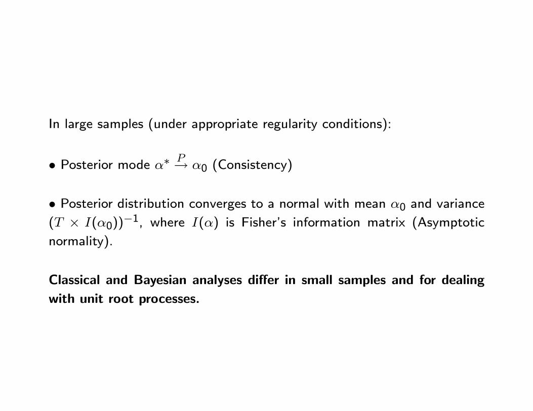
In large samples (under appropriate regularity conditions):

• Posterior mode α∗ P→ α0 (Consistency)

• Posterior distribution converges to a normal with mean α0 and variance

(T × I(α0))−1, where I(α) is Fisher’s information matrix (Asymptotic

normality).

Classical and Bayesian analyses differ in small samples and for dealing

with unit root processes.

Bayesian analysis requires:

• Initial information → Prior distribution.

• Data → Likelihood.

• Prior and Likelihood → Bayes theorem → Posterior distribution.

• Can proceed recursively (mimic economic learning).

• f(y) it is a measure of fit. It tells us how good the model is in reproducing

the data, not at a single point, but on average over the parameter space.

• α are regression coefficients, structural parameters, etc.; g(α|y) is the

conditional probability of α, given what we observe, y.

• Theorem uses rule: P (A,B) = P (A|B)P (B) = P (B|A)P (A). It says

that if we start from some beliefs on α, we may modify them if we observe

y. It does not says what the initial beliefs are, but how they should change

is data is observed.

To use Bayes theorem we need:

a) Formulate prior beliefs, i.e. choose g(α).

b) Formulate a model for the data (the conditional probability of f(y|α)).

After observing the data, we treat the model as the likelihood of α condi-

tional on y, and update beliefs about α.

• Bayes theorem with nuisance parameters (e.g. α1 long run coefficients,

α2 short run coefficients; α1 regression coefficient; α2 serial correlation

coefficient in the errors).

Let α = [α1, α2] and suppose interest is in α1. Then g(α1, α2|y) ∝f(y|α1, α2)g(α1, α2)

g(α1|y) =∫g(α1, α2|y)dα2

=∫g(α1|α2, y)g(α2|y)dα2 (1)

Posterior of α1 averages the conditional of α1 with weights given by the

posterior of α2.

• Bayes Theorem with two (N) samples.

Suppose yt = [y1t, y2t] and that y1t is independent of y2t. Then

g ≡ f(y1, y2|α)g(α) = f2(y2|α)f1(y1|α)g(α) ∝ f2(y2|α)g(α|y1) (2)

Posterior for α is obtained finding first the posterior of using y1t and then,

treating it as a prior, finding the posterior using y2t.

- Sequential learning.

- Can use data from different regimes.

- Can use data from different countries.

2.1 Likelihood Selection

• It should reflect an economic model.

• It must represent well the data. Misspecification problematic since it

spills across equations and makes estimates uninterpretable.

• For our purposes the likelihood is simply the theoretical (DSGE) model

you write down.

2.2 Prior Selection

• Three methods to choose priors in theory. Two not useful for DSGE

models since are designed for models which are linear in the parameters.

1) Non-Informative subjective. Choose reference priors because they are

invariant to the parametrization.

- Location invariant prior: g(α) =constant (=1 for convenience). Scale

invariant prior g(σ) = σ−1.

- Location-scale invariant prior : g(α, σ) = σ−1.

• Non-informative priors useful because many classical estimators (OLS,

ML) are Bayesian estimators with non-informative priors

2) Conjugate Priors

A prior is conjugate if the posterior has the same form as the prior. Hence,

the form posterior will be analytically available, only need to figure out its

posterior moments.

• Important result in linear models with conjugate priors: Posterior mo-

ments = weighted average of sample and prior information. Weights =

relative precision of sample and prior informations.

Tight Prior

4 2 0 2 40.0

0.5

1.0

1.5

2.0POSTERIORPRIOR

Loose Prior

4 2 0 2 40.0

0.5

1.0

1.5

2.0POSTERIORPRIOR

Important:

- y1, . . . yT should not be the same sample used for inference.

- y1, . . . yT could represent past time series information, cross sectional/

cross country information.

- Typically y1, . . . yT is called ”Training sample”.

4) Priors for DSGE - similar to MLII priors.

- Assume that g(α) = g1(α1)g2(α2)....gq(αq).

- Use a conventional format for the distributions: a Normal, Beta and

Gamma for individual parameters. Choose moments in a data based fash-

ion: mean = calibrated parameters, variance: subjective.

Problems:

• Independent priors typically inconsistent with any subjective prior beliefs

over joint outcomes. In particular, multivariate priors are often too tight!!

• Calibrated value may be different for different purposes. For example,

risk aversion mean is 6-10 to fit the equity premium; close to 1-2 if we

want to fit the reaction of consumption to changes in monetary policy;

negative values to fit aggregate lottery revenues. Which one do we use?

Same for habit parameters (see Faust and Gupta, 2012)

• Circularity: priors based on the same data used to estimate!! Use cali-

brated values in a ” training sample”.

See later del Negro and Schorfheide (2008) for formally choosing data

based priors in training samples which are not independent.

Summary

Inputs of the analysis: g(α), f(y|α).

Outputs of the analysis:

g(α|y) ∝ f(y|α)g(α) (posterior),

f(y) =∫f(y|α)g(α) (marginal likelihood), and

f(yT+τ |yT ) (predictive density of future observations).

Likelihood should reflect data/ economic theory.

Prior could be non-informative, conjugate, data based (objective).

- In simple examples, f(y) and g(α|y) can be computed analytically.

- In general, can only be computed numerically by Monte Carlo methods.

- If the likelihood is a (log-linearized) DSGE model: always need numerical

computations.

3 Posterior simulators

Objects of interest for Bayesian analysis: E(h(α)) =∫h(α)g(α|y)dα. Oc-

casionally, can evaluate the integral analytically. In general, it is impossible.

If g(α|y) were available: we could compute E(h(α)) with MC methods:

- Draw αl from g(α|y). Compute h(αl)

- Repeat draw L times. Average h(αl) over draws.

Example 3.1 Suppose we are interested in computing Pr(α > 0). Draw

αl from g(α|y). If αl > 0, set h(αl) = 1, else set h(αl) = 0. Draw L times

and average h(αl) over draws. The result is an estimate of Pr(α > 0).

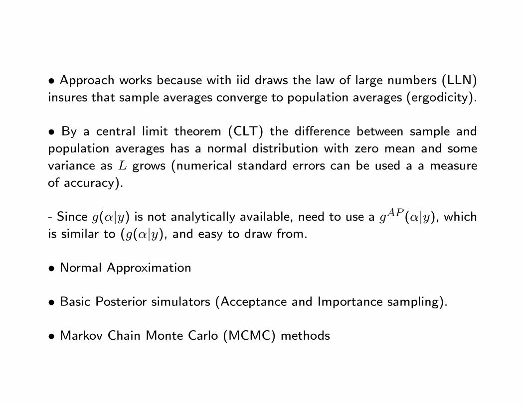
• Approach works because with iid draws the law of large numbers (LLN)

insures that sample averages converge to population averages (ergodicity).

• By a central limit theorem (CLT) the difference between sample and

population averages has a normal distribution with zero mean and some

variance as L grows (numerical standard errors can be used a a measure

of accuracy).

- Since g(α|y) is not analytically available, need to use a gAP (α|y), which

is similar to (g(α|y), and easy to draw from.

• Normal Approximation

• Basic Posterior simulators (Acceptance and Importance sampling).

• Markov Chain Monte Carlo (MCMC) methods

• Approximation is valid under regularity conditions when T →∞ or when

the posterior kernel is roughly normal. It is highly inappropriate when:

- Likelihood function flat in some dimension (I(α∗) badly estimated).

- Likelihood function is unbounded (no posterior mode exists).

- Likelihood function has multiple peaks.

- α∗ is on the boundary of A (quadratic approximation wrong).

- g(α) = 0 in a neighborhood of α∗ (quadratic approximation wrong).

How do we construct a normal approximation?

A) Find the mode of the posterior.

max log g(α|y) = max(logL(α|y) + log g(α))

- Problem is identical to the one of finding the maximum of a likelihood.

The objective function differs.

Two mode finding algorithms:

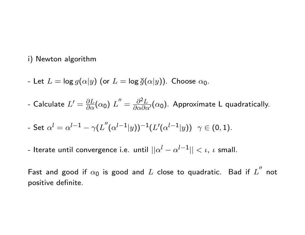
i) Newton algorithm

- Let L = log g(α|y) (or L = log g(α|y)). Choose α0.

- Calculate L′ = ∂L∂α(α0) L

′′= ∂2L

∂α∂α′(α0). Approximate L quadratically.

- Set αl = αl−1 − γ(L′′(αl−1|y))−1(L′(αl−1|y)) γ ∈ (0, 1).

- Iterate until convergence i.e. until ||αl − αl−1|| < ι, ι small.

Fast and good if α0 is good and L close to quadratic. Bad if L′′

not

positive definite.

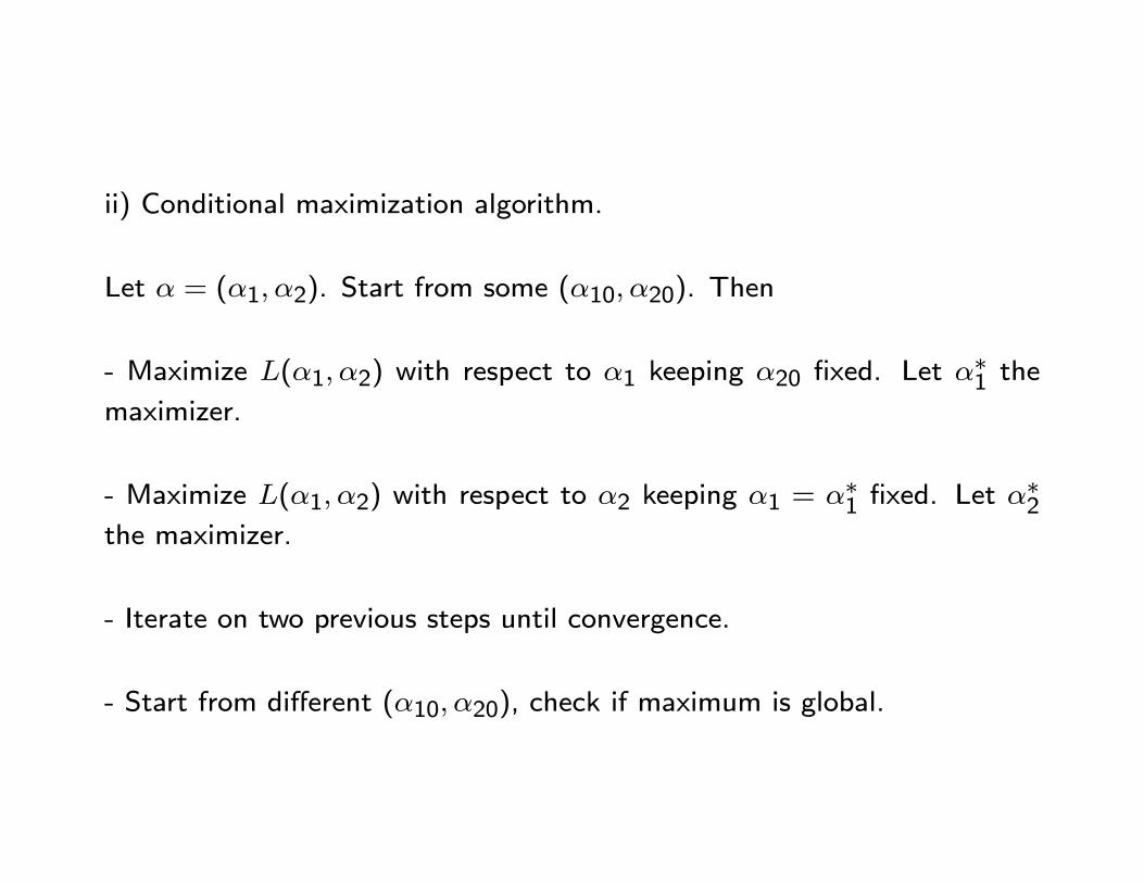
ii) Conditional maximization algorithm.

Let α = (α1, α2). Start from some (α10, α20). Then

- Maximize L(α1, α2) with respect to α1 keeping α20 fixed. Let α∗1 the

maximizer.

- Maximize L(α1, α2) with respect to α2 keeping α1 = α∗1 fixed. Let α∗2the maximizer.

- Iterate on two previous steps until convergence.

- Start from different (α10, α20), check if maximum is global.

B) Compute the variance covariance matrix at the mode

- Use the Hessian Σα∗ = −[∂2 log g(α|y)

∂α∂α′−1|α=α∗]

C) Approximate the posterior density around the mode: gAP (α|y) =N(α∗,Σα∗).

- If multiple modes are present, find an approximation to each mode, andset gAP (α|y) =

∑i %iN(α∗i ,Σα∗i ) where 0 ≤ %i ≤ 1. If modes are clearly

separated select %i = g(α∗i |y)|Σα∗i |−0.5.

- If the sample is small, use a t-approximation i.e. gAP (α|y) =∑i %ig(α|y)[ν + (α− α∗i )′Σαi(α− α∗i )]−0.5(k+v) with small ν.

(If ν = 1 t-distribution=Cauchy distribution, large overdispersion. Typi-cally ν = 4, 5 appropriate).

D) To conduct inference, draw αl from gAP (α|y).

If draws are iid, E(h(α)) = 1L

∑l h(αl). Use LLN to approximate any pos-

terior probability contours of h(α), e.g. a 16-84 range is [h(α16), h(α84)].

E) Check accuracy of approximation.

Compute Importance Ratio IRl =g(αl|y)gAP (αl|y)

. Accuracy is good if IRl is

constant across l. If not, need to use other techniques.

Note: Importance ratios are not automatically computed in Dynare. Need

to do it yourself.

Example 3.2 True: g(α|y) is t(0,1,2). Approximation: N(0,c), where c = 3, 5, 10, 100.

100 200 300 400 5000

200

400

600

800

c=3

Fre

quen

cy

1 2 30

50

100

c=5

0.5 1 1.5 2 2.50

50

100

c=10

Weights

Fre

quen

cy

2 4 6 80

50

100

c=100

Weights

Horizontal axis=importance ratio weights, vertical axis= frequency of the weights.

- Posterior has fat tails relative to a normal (poor approximation).

3.2 Basic Posterior Simulators

• Draw from a general gAP (α|y) (not necessarily normal).

• Non-iterative methods - gAP (α|y) is fixed across draws.

• Work well when IRl is roughly constant across draws.

A) Acceptance sampling

B) Importance sampling

3.3 Markov Chain Monte Carlo Methods

• Problem with basic simulators: approximating density is selected once

and for all. If mistakes are made, they stay. With MCMC location of

approximating density changes as iterations progress.

• Idea: Suppose n states (x1, . . . xn). Let P (i, j) = Pr(xt+1 = xj|xt =

xi) and let µ(t) = (µ1t, . . . µnt) be the unconditional probability at t of

each state n. Then µ(t + 1) = Pµ(t) = P tµ(0) and µ is an equilibrium

(ergodic, steady state, invariant) distribution if µ = µP .

Set µ = g(α|y), choose some initial density µ(0) and some transition

P across states. If conditions are right, iterate from µ(0) and limiting

distribution is g(α|y), the unknown posterior.

g(α|y)

gMC(1)

gMC(0)

α

• Under general conditions, the ergodicity of P insures consistency and

asymptotic normality of estimates of any h(α).

Need a transition P (α,A), where A is some set, such that ||P (α,A) −µ(α)|| → 0 in the limit. For this need that the chain associated with P :

• is irreducible, i.e. it has no absorbing state.

• is aperiodic, i.e. it does not cycle across a finite number of states.

• it is Harris recurrent, i.e. each cell is visited an infinite number of times

with probability one.

Bad draws Good draws

A B ABB

Result 1: A reversible Markov chain, has an ergodic distribution (exis-

tence). (if µiPi,j = µjPj,i then (µP )j =∑j µiPi,j =

∑i µjPj,i =

µj∑i Pj,i = µj.)

Result 2: (Tierney (1994)) (uniqueness) If a Markov chain is Harris recur-

rent and has a proper invariant distribution. µ(α), µ(α) is unique.

Result 3: (Tierney(1994)) (convergence) If a Markov chain with invariant

µ(α) is Harris recurrent and aperiodic, for all α0 ∈ A and all A, as L→∞.

- ||PL(α0, A)− µ(α)|| → 0, ||.|| is the total variation distance.

- For all h(α) absolutely integrable with respect to µ(α).

- limL→∞1L

∑Ll=1 h(αl)

a.s.→∫h(α)µ(α)dα.

If chain has a finite number of states, it is sufficient for the chain to

be irreducible, Harris recurrent and aperiodic that P (αl ∈ A1|αl−1 =

α0, y) > 0, all α0, A1 ∈ A.

• Can dispense with the finite number of state assumption.

• Can dispense with the first order Markov assumption.

General simulation strategy:

• Choose starting values α0, choose a P with the right properties.

• Run MCMC simulations.

• Check convergence.

• Summarize results i.e compute h(α).

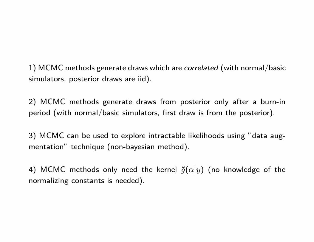
1) MCMC methods generate draws which are correlated (with normal/basic

simulators, posterior draws are iid).

2) MCMC methods generate draws from posterior only after a burn-in

period (with normal/basic simulators, first draw is from the posterior).

3) MCMC can be used to explore intractable likelihoods using ”data aug-

mentation” technique (non-bayesian method).

4) MCMC methods only need the kernel g(α|y) (no knowledge of the

normalizing constants is needed).

3.3.1 Metropolis-Hastings algorithm

MH is a general purpose MCMC algorithm that can be used when faster

methods (such as the Gibbs sampler) are either not usable or difficult to

implement.

Starts from an arbitrary transition function q(α†, αl−1), where αl−1, α† ∈A and an arbitrary α0 ∈ A. For each l = 1, 2, . . . L.

- Draw α† from q(α†, αl−1) and draw $ ∼ U(0, 1).

- If $ < E(αl−1, α†) = [g(α†|Y )q(α†,αl−1)g(αl−1|Y )q(αl−1,α†)

], set α` = α†.

- Else set α` = α`−1.

These iterations define a mixture of continuous and discrete transitions:

P (αl−1, αl) = q(αl−1, αl)E(αl−1, αl) if αl 6= αl−1

= 1−∫Aq(αl−1, α)E(αl−1, α)dα if αl = αl−1 (6)

P (αl−1, αl) satisfies the conditions needed for existence, uniqueness and

convergence.

• Idea: Want to sample from highest probability region but want to visit

as much as possible the parameter space. How to do it? Choose an initial

vector and a candidate, compute kernel of posterior at the two vectors. If

you go uphill, keep the draw, otherwise keep the draw with some probability.

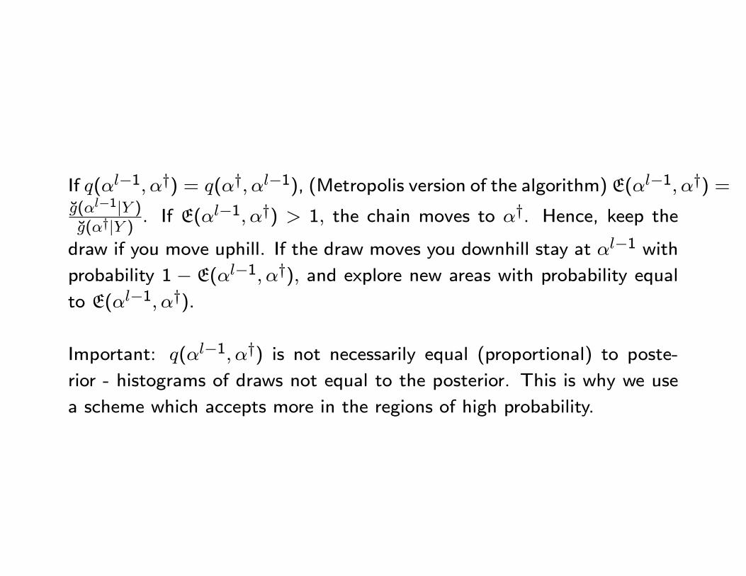
If q(αl−1, α†) = q(α†, αl−1), (Metropolis version of the algorithm) E(αl−1, α†) =g(αl−1|Y )g(α†|Y )

. If E(αl−1, α†) > 1, the chain moves to α†. Hence, keep the

draw if you move uphill. If the draw moves you downhill stay at αl−1 with

probability 1 − E(αl−1, α†), and explore new areas with probability equal

to E(αl−1, α†).

Important: q(αl−1, α†) is not necessarily equal (proportional) to poste-

rior - histograms of draws not equal to the posterior. This is why we use

a scheme which accepts more in the regions of high probability.

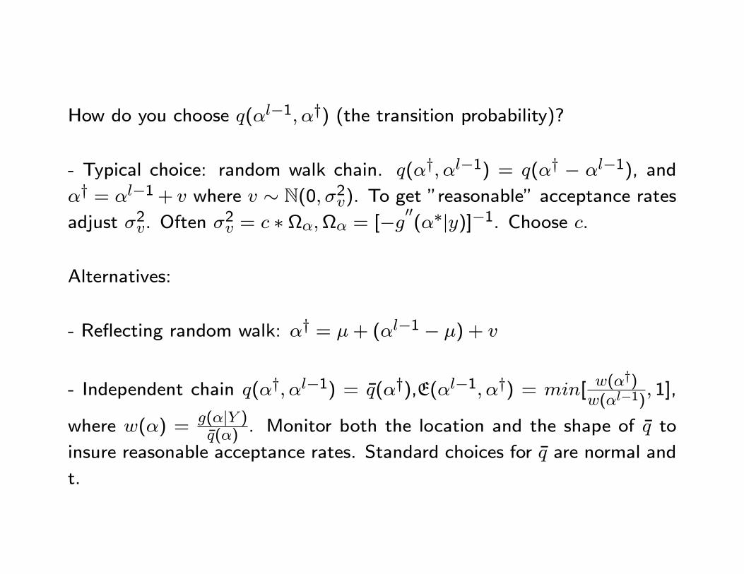
How do you choose q(αl−1, α†) (the transition probability)?

- Typical choice: random walk chain. q(α†, αl−1) = q(α† − αl−1), and

α† = αl−1 + v where v ∼ N(0, σ2v). To get ”reasonable” acceptance rates

adjust σ2v. Often σ2

v = c ∗ Ωα,Ωα = [−g′′(α∗|y)]−1. Choose c.

Alternatives:

- Reflecting random walk: α† = µ+ (αl−1 − µ) + v

- Independent chain q(α†, αl−1) = q(α†),E(αl−1, α†) = min[w(α†)w(αl−1)

, 1],

where w(α) =g(α|Y )q(α)

. Monitor both the location and the shape of q to

insure reasonable acceptance rates. Standard choices for q are normal and

t.

• General rule for selecting q. A good q must:

a) be easy to sample from

b) be such that it is easy to compute E.

c) each move goes a reasonable distance in parameter space but does not

reject too frequently (ideal rejection rate 30-50%).

Implementation issues

A) How to draw samples?

- Produce one sample (of dimension n ∗ L + L). Throw away initial L

observations. Keep only elements (L, 2L, . . . , n ∗ L) (to eliminate the

serial correlation of the draws).

- Produces n samples of L+ L elements. Use last L observations in each

sample for inference.

- Dynare setup to produce n samples, keep the last 25 percent of the

draws. Careful: Need to make sure that with 75 percent of the draws

the chain has converged.

B) How long should be L? How do you check convergence?

- Start from different α0. Check if sample you keep, for a given L, has

same properties (Dynare approach).

- Choose two points, L1 < L2; compute distributions/moments of α after

these points. If visually similar, algorithm has converged at L1. Could

this recursively → CUMSUM statistic for mean, variance, etc.(checks if it

settles down, no testing required).

For simple problems L ≈ 50 and L ≈ 200.

For DSGEs L ≈ 100, 000− 200, 000 and L ≈ 500, 000. If Multiple modes

are present L could be even larger.

C) Inference : easy.

- Weak Law of Large Numbers E(h(α)) ≈ 1j

∑nj=1 h(αjL), where αjL is

the j ∗ L-th observation drawn after L iterations are performed.

- E(h(α)h(α)′) =∑J(L)−J(L)w(τ)ACFh(τ); ACFh(τ) = autocovariance of

h(α) for draws separated by τ periods; J(L) function of L, w(τ) a set of

weights.

- Marginal density (α1k, . . . α

Lk ): g(αk|y) = 1

L

∑Lj=1 g(αk|y, α

jk′, k

′ 6= k).

- Predictive inference f(yt+τ |yt) =∫f(yt+τ |yt, α)g(α|yt)dα.

- Model comparisons: compute marginal likelihood numerically.

4 Robustness

• Typically prior chosen to make calculation convenient. How sensitive areresults to prior choice?

• Typical (brute force) approach: repeat estimation for different priors(inefficient).

• Alternative.

i) Select an alternative prior g1(α) with support included in g(α).

ii) Let w(α) =g(α)g1(α)

. Then any h1(α) =∫

(h(α)w(α)dg1(α) can be

approximated using h1(α) ≈1L

∑lw(αl)h(αl)∑lw(αl)

.

•Just need the original output obtained and a set of weigths!

Example 4.1 yt = xtα+ut ut ∼ (0, σ2). Suppose g(α) is N(0, 10). Then

g(α|Y ) is normal with mean α = Σ−1(0.1 + σ−2x′xαols) and variance

Σ = 0.1 + σ−2x′x, . If one wishes to examine how forecasts of the model

change when the prior variances changes (for example to 5) two alternatives

are possible:

(a) draw from normal g(α|Y ) which has mean α1 = Σ−11 (0.2+σ−2x′xαols)

and variance Σ = 0.2 + σ−2x′x, and compare forecasts.

(b) Weight draws from the initial posterior distribution withg(α)g1(α)

where

g1(α) is N(0, 5).

5 Bayesian estimation of DSGE models

Why using Bayesian methods to estimate DSGE models?

1) Hard to include non-sample information in classical ML (a part from

range of possible values).

2) Classical ML is justified only if the model is the GDP of the actual data.

Can use Bayesian methods for misspecified models (economic inference

may be problematic, no problem for statistical inference).

3) Can incorporate prior uncertainty about parameters and models.

General Principles:

• Use the fact that (log-)linearized DSGE models are state space models

whose reduced form parameters α are nonlinear functions of structural θ.

Compute the likelihood via the Kalman filter.

• Posterior of θ can be obtained using MH algorithm.

• Use posterior output to compute the marginal likelihood, Bayes factors

and any posterior function of the parameters (impulse responses, ACF,

turning point predictions, forecasts, etc.).

• Check robustness to the choice of prior.

General algorithm: Given θ0

[1.] Construct a log-linear solution of the DSGE economy.

[2.] Specify prior distributions g(θ).

[3.] Transform the data to make sure that is conformable with the model.

[4.] Compute likelihood via Kalman filter.

[5.] Draw sequences for θ using MH algorithm. Check convergence.

[6.] Compute marginal likelihood and compare it to the one of alternative

models. Compute Bayes factors.

[7.] Construct statistics of interest. Use loss-based evaluation of discrep-

ancy model/data.

[8.] Perform robustness exercises.

Step 1.: can have nonlinear state space models (see later and e.g. Amisano

and Tristani (2006), Rubio and Villaverde (2009)) or value function prob-

lems (see Bi and Traum (2012)) but computations much more complex.

System are typically singular! Need to:

i) add measurement errors if want to use all observables (where to put mea-

surement error? In all variables or just enough to complete the probability

space?)

ii) find a way to reduce the dimensionality of the system (substituting

equations before the solution is computed).

iii) choose the observables optimally (see Canova et al. (2012)).

iv) invent new structural shocks.

In Step 3. transformations are needed because the model is typically solved

in deviation from the steady states. Need to eliminate from the data any

long run component. How do you do it? Many ways of doing this (see

Canova, 2010) all unsatisfactory.

Step 4 is typically the most computationally intensive step. Considerable

gains if this is efficiently done.

In step 5. Given θl

i) Draw a θ† from the P(θ†θl). Solve the model.

ii) Use the KF to compute the likelihood.

iii) Evaluate the posterior kernel at the draw g(θ†|y) = f(y|θ†)g(θ†).

iv) Evaluate the posterior kernel at θl i.e g(θ0|y) = f(y|θl)g(θl).

v) Compute IR =g(θ†)g(θl)

P(θl,θ†)P(θ†,θl)

. If IR > 1 set θl+1 = θ†.

vi) Else draw $ ∼ U(0, 1). If $ < IR set θl+1 = θ† otherwise set

θl+1 = θl.

vii) Repeat i)-vi) L + nL times. Throw away L draws. Keep one every n

for inference.

In Step 6. use a modified harmonic mean estimator i.e. approximate

L(yt|Mi) using [ 1L

∑l

f(αil)

L(yt|αil,Mi)g(αil|Mi)]−1 where αli is the draw l of the

parameters α of model i and f is a density with tails thicker than a normal.

If f(αil) = 1 we have a simple harmonic mean estimator.

Competitors could be a more densely parametrized structural model (nest-

ing the interested one) or more densely parametrized reduced form model

(e.g. VAR or a BVAR).

Bayes factors can be computed numerically or via Laplace approximations

(to decrease computational burden in large scale systems).

In step 7 Estimate marginal/ joint posteriors using kernel methods. Com-

pute point estimate and credible sets. Compute continuous functions h(θ)

of interest. Set up a loss function. Compare models using the risk function.

In step 8. Reweight the draws appropriately.

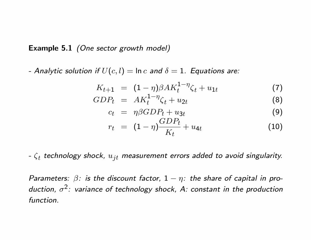
Example 5.1 (One sector growth model)

- Analytic solution if U(c, l) = ln c and δ = 1. Equations are:

Kt+1 = (1− η)βAK1−ηt ζt + u1t (7)

GDPt = AK1−ηt ζt + u2t (8)

ct = ηβGDPt + u3t (9)

rt = (1− η)GDPt

Kt+ u4t (10)

- ζt technology shock, ujt measurement errors added to avoid singularity.

Parameters: β: is the discount factor, 1 − η: the share of capital in pro-

duction, σ2: variance of technology shock, A: constant in the production

function.

Simulate 1000 points from using k0 = 100.0 using A = 2.86; 1 − η =

0.36;β = 0.99, σ2 = (0.07)2.

Assume u1t ∼ N(0, 0.12); um2t ∼ N(0, 0.062);um3t ∼ N(0, 0.022);

um4t ∼ N(0, 0.082); (Note: lots of measurement error!)

- Keep last 160 as data (to mimic about 40 years of quarterly data).

Interested in (1− η), β i.e (treat σ2, A as fixed).

Use (9)-(10) to identify the parameters from the data.

Priors: (1 − η) ∼ Beta(3,5); β ∼ Beta(98,2) (NOTATION DIFFERENT

FROM DYNARE)

Mean of a Beta(a,b) is (a/a+b) and the variance of a Beta(a,b)is ab/[(a+

b)2 ∗ (a+ b+ 1)]. Thus prior mean of 1− η = 0.37, prior variance 0.025;

prior mean of β = 0.98, prior variance 0.0001.

Let θ = (1 − η, β) Use random walk to draw θ†, i.e. θ† = +θl−1 + e†,µ is the mean and ei is U(−0.08, 0.08) for β and U(−0.06, 0.06) for η

(roughly about 28% acceptance rate).

Draw 10000 replications from the posterior kernel. Convergence is fast.

Keep last 5000; use one every 5 for inference.

1eta

0.1 0.2 0.3 0.4 0.5 0.6 0.70

1

2

3

4

5

6PRIORPOSTERIOR

beta

0.900 0.925 0.950 0.975 1.0000

5

10

15

20

25

30

35

40PRIORPOSTERIOR

Figure 4: Priors and Posteriors, RBC model

- Prior for β sufficiently loose, posterior similar, data is not very formative.

-Posteriors centered around the true parameters,large dispersion.

Variances/covariancestrue posterior 68% range

var(c) 0.24 [ 0.11, 0.27]var(y) 0.05 [ 0.03, 0.11]cov(c,y) 0.0002 [ 0.0003, 0.0006]

Wrong model

- Simulate data from model with habit γ = 0.8

- Estimate model conditioning on γ = 0.

1eta

0.00 0.25 0.50 0.75 1.000

1

2

3

4

5

6PRIORPOSTERIOR

beta

0.6 0.7 0.8 0.9 1.00

5

10

15

20

25

30

35

40PRIORPOSTERIOR

Figure 5: Priors and Posteriors, wrong model

Example 5.2 (New Keynesian model)

gapt = Etgapt+1 −1

ϕ(rt − Etπt+1) + gt (11)

πt = βEtπt+1 + κgapt + vt (12)

rt = φrrt−1 + (1− φr)(φππt−1 + φgapgapt−1) + et (13)

κ =(1−ζp)(1−βζp)(ϕ+ϑN)

ζp; ζp = degree of (Calvo) stickiness, β = discount

factor, ϕ = risk aversion, ϑN = elasticity of labor supply. gt and vt are

AR(1) with persistence ρg, ρv and variances σ2g, σ

2v; et ∼ iid(0, σ2

r).

θ = (β, ϕ, ϑl, ζp, φπ, φgap, φr, ρg, ρv, σ2v, σ

2g, σ

2r).

Assume g(θ) =∏g(θi)

Assume β ∼ Beta(98, 3), ϕ ∼ N(1, 0.3752), ϑN ∼ N(2, 0.752), ζp ∼Beta(9, 3), φr ∼ Beta(6, 2), φπ ∼ Normal(1.5, 0.12),

φgap ∼ N(0.5, 0.052), ρg ∼ Beta(17, 3), ρv ∼ Beta(17, 3) σ2i ∼ IG(2, 0.01), i =

g, v, r.

Use US linearly detrended data from 1948:1 to 2002:1 to estimate the

model.

Use random walk MH algorithm to draw candidates.

0 50 100 150 200 2508

8.5

9

9.5y

0 50 100 150 200 2500.02

0

0.02

0.04π

0 50 100 150 200 25000.01

0.02

0.030.04

r

Figure 6: Raw Time series

0 0.5 1 1.5 2x 10 4

1

0

1

2beta

0 0.5 1 1.5 2x 10 4

0.5

0

0.5varphi

0 0.5 1 1.5 2x 10 4

0.5

0

0.5vartheta(N)

zeta(p)

0 0.5 1 1.5 2x 10 4

0.5

0

0.5

0 0.5 1 1.5 2x 10 4

0.5

0

0.5phi(r)

0 0.5 1 1.5 2x 10 4

1.5

1

0.5

0phi(pi)

0 0.5 1 1.5 2x 10 4

0

1

2

3phi(gap)

0 0.5 1 1.5 2x 10 4

0.5

0

0.5rho(4)

0 0.5 1 1.5 2x 10 4

0.5

0

0.5rho(2)

0 0.5 1 1.5 2x 10 4

0.5

0

0.5sig(4)

0 0.5 1 1.5 2x 10 4

0.5

0

0.5sig(2)

0 0.5 1 1.5 2x 10 4

0.5

0

0.5sig(3)

Figure 7: CUMSUM statistics

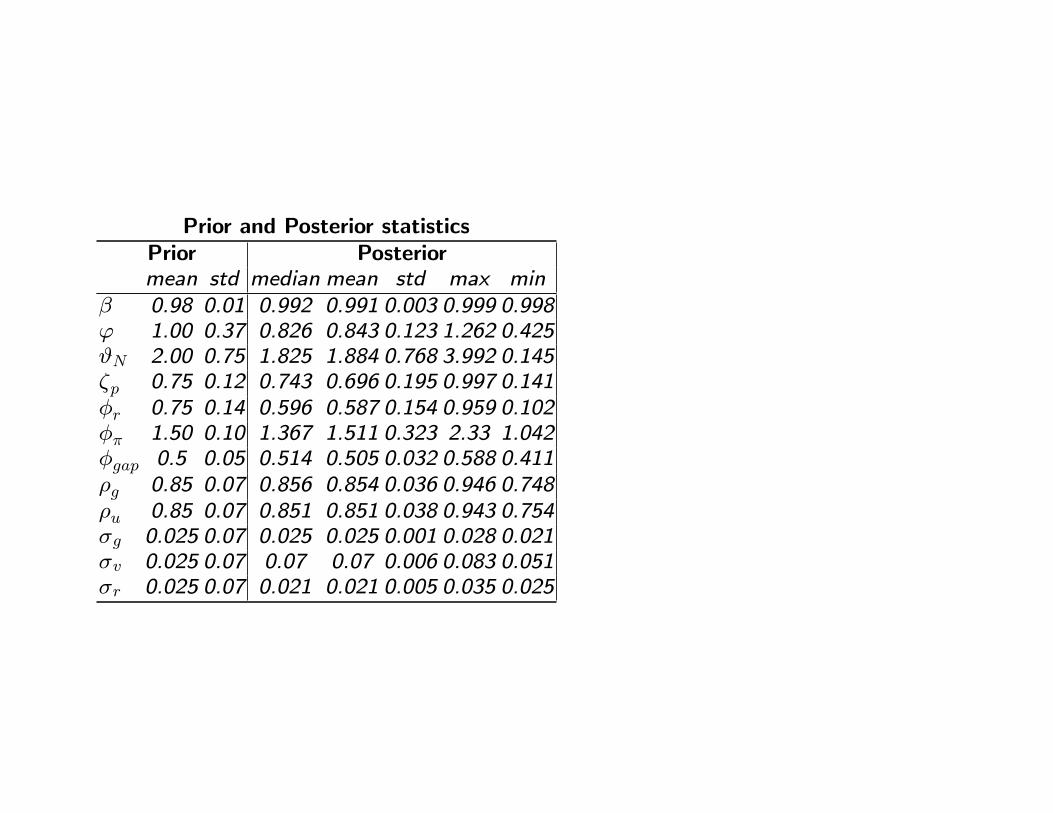
Prior and Posterior statisticsPrior Posteriormean std median mean std max min

β 0.98 0.01 0.992 0.991 0.003 0.999 0.998ϕ 1.00 0.37 0.826 0.843 0.123 1.262 0.425ϑN 2.00 0.75 1.825 1.884 0.768 3.992 0.145ζp 0.75 0.12 0.743 0.696 0.195 0.997 0.141φr 0.75 0.14 0.596 0.587 0.154 0.959 0.102φπ 1.50 0.10 1.367 1.511 0.323 2.33 1.042φgap 0.5 0.05 0.514 0.505 0.032 0.588 0.411ρg 0.85 0.07 0.856 0.854 0.036 0.946 0.748ρu 0.85 0.07 0.851 0.851 0.038 0.943 0.754σg 0.025 0.07 0.025 0.025 0.001 0.028 0.021σv 0.025 0.07 0.07 0.07 0.006 0.083 0.051σr 0.025 0.07 0.021 0.021 0.005 0.035 0.025

- Little information in the data for some parameters (prior and posterior

overlap).

- For parameters of the policy rule: posteriors move and not more concen-

trated.

-Posterior distributions roughly symmetric except for φπ and ζp (mean and

median coincide).

-Posterior distribution of economic parameters reasonable (except ϕ).

- Posterior for the AR parameters has a high mean, but no pile up at one.

0.9 1 1.10

0.5

1beta

0 0.5 1 1.5 20

0.5

1varphi

0 2 4 60

0.5

1 vartheta(N)

0 0.5 10

0.5

1 zeta(p)

0 0.5 10

0.5

1phi(r)

1.5 2 2.50

0.5

1phi(pi)

0 0.2 0.4 0.6 0.80

0.5

1 phi(gap)

0.6 0.8 1 1.20

0.5

1rho(4)

0.6 0.8 1 1.20

0.5

1rho(2)

0 0.02 0.04 0.06 0.080

0.5

1sig(4)

0 0.02 0.04 0.06 0.080

0.5

1sig(2)

0 0.02 0.04 0.06 0.080

0.5

1sig(3)

Figure 8: Priors and Posteriors, NK model

Model comparisons

Compare ML against flat prior VAR(3) or a BVAR(3) with Minnesota prior

and standard parameters (tightness=0.1, linear lag decay and weight on

other variables equal 0.5), both with a constant.

Bayes factor are very small ≈ 0.02 in both cases.

• The restrictions the model imposes are false. Need to add features to

the model that make dynamics of the model more similar to those of a

VAR(3).

Posterior analysis

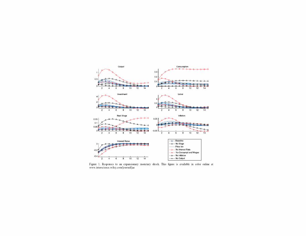
How do responses to monetary shocks look like? No persistence!

0 5 102.5

2

1.5

1

0.5

0Output gap

0 5 106

5

4

3

2

1

0

Horizon (Quarters)

Prices

0 5 100.5

0

0.5

1Nominal rate

How much of the output gap and inflation variance explained by monetary

shocks? Almost all!!

5.1 Interpreting results

- Most of the shocks of DSGE models are non-structural (alike to measure-

ment errors). Careful with interpretation and policy analyses with these

models (see Chari et al. (2009)).

- A model where ”measurement errors” explain a large portion of main

macro variables is very suspicious (e.g. in Smets and Wouters (2003)

markup shocks dominate).

- If the standard error of one the shocks is large relative to the others:

evidence of misspecification.

- Compare estimates with standard calibrated values. Are they sensible?

Often yes, but because of tight priors are centered at calibrated values.

5.2 Bayesian methods and identification

Likelihood of a DSGE typically flat. Could be due to marginalization (use

only a subset of economic relationships), or to lack of information. Difficult

to say a-priori which parameters is underidentified and which is not (since

we do not have an analytic solution).

Could go a long way by numerically constructing the likelihood as a function

of the parameters (see Canova and Sala (2009)).

Standard remedy when some parameters are hard to identify: calibrate.

Problem if parameter not fixed at a consistent estimator → biases could

be extensive! (see Canova and Sala (2009)).

Alternative: add a prior. This increases the curvature of the likelihood →underidentification may be hidden!. Posterior look nice because the prior

does the job!!.

In general if L(θ1, θ2|Y T ) = L(θ1|Y T ) then g(θ1, θ2|Y T ) = g1(θ1|Y T )

g(θ2|θ1), i.e no updating of conditional prior of θ2.

However, updating possible even if no sample information is present if

θ1, θ2 are linked by economic or stability conditions!!

0.010.02

0.03

0.985

0.99

0.995

20

15

10

5

0x 10 4

δβ0.01

0.020.03

0.985

0.99

0.995

43.5

32.5

21.5

10.5

0

x 10 4

δβ

Likelihood and Posterior, δ and β in a RBC model

If prior ≈ posterior: weak identification or too much data based prior?

6 Topics

6.1 Eliciting Priors from existing information

- Prior distributions for DSGE parameters often arbitrary.

- Prior distribution for individual parameters assumed to be independent: the joint dis-

tribution may assign non-zero probability to ” unreasonable” regions of the parameter

space.

- Prior sometimes set having some statistics in mind (the prior mean is similar to the one

obtained in calibration exercises).

- Same prior is used for the parameters of different models. Problem: same prior may

generate very different dynamics in different models. Hard to compare the outputs.

Example 6.1 Let yt = θ1yt−1 + θ2 + ut, ut ∼ N(0, 1).. Suppose θ1 and θ2 are

independent and p(θ1) ∼ U(0, 1− ε), ε > 0; p(θ2|θ1) ∼ N(µ, λ).

Since the mean of yt is µ = θ2

1−θ1, the prior for θ1 and θ2 imply that µ|θ1 ∼ N(µ, λ

(1−θ1)2 ).

Hence, the prior mean of yt has a variance which is increasing in the persistence parameter

θ1! Why? Reasonable ?

Alternative: state a prior for µ, derive the prior for θ1 and θ2 (change of variables). For

example, if µ ∼ N(µ, λ2) then p(θ1) = U(0, 1− ε), p(θ2|θ1) = N(µ(1−θ1), λ2(1−θ1)2).

Note here that the priors for θ1 and θ2 are correlated.

Suppose you want to compare the model with yt = θ + ut, ut ∼ N(0, 1). If p(θ) =

N(µ, λ2) the two models are immediately comparable. If, instead, we had assumed

independent priors for p(θ1) and p(θ2), the two models would not be comparable (standard

prior has weird predictions for the prior of the mean of yt).

- Del Negro and Schorfheide (2008): elicit priors consistent with some

distribution of statistics of actual data (see also Kadane et al. (1980)).

Basic idea:

i) Let θ be a set of DSGE parameters. Let ST be a set of statistics obtained

in the data with T observations and σS be the standard deviation of these

statistics (which can be computed using asymptotic distributions or small

sample devices, such as bootstrap or MC methods).

ii) Let SN(θ) be the same set of statistics which are measurable from the

model once θ is selected using N observations. Then

ST = SN(θ) + η η ∼ (0,ΣTN) (14)

where η is a set of measurement errors.

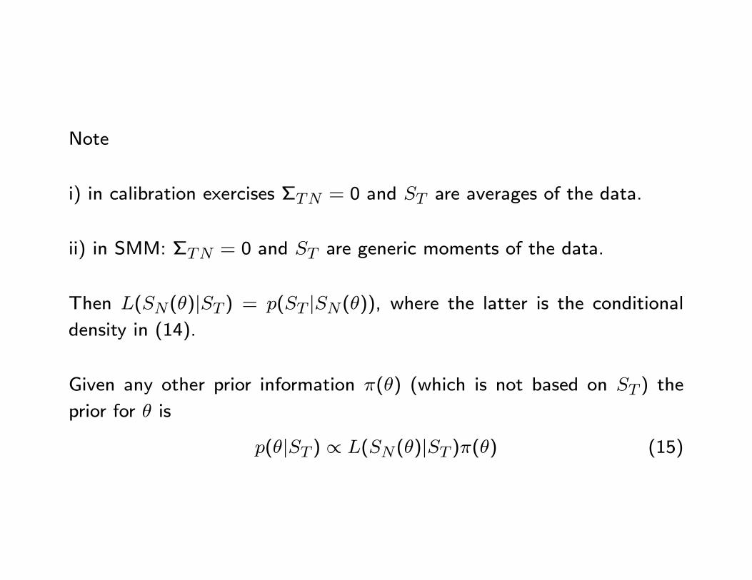
Note

i) in calibration exercises ΣTN = 0 and ST are averages of the data.

ii) in SMM: ΣTN = 0 and ST are generic moments of the data.

Then L(SN(θ)|ST ) = p(ST |SN(θ)), where the latter is the conditional

density in (14).

Given any other prior information π(θ) (which is not based on ST ) the

prior for θ is

p(θ|ST ) ∝ L(SN(θ)|ST )π(θ) (15)

- dim(ST ) ≥ dim(θ): overidentification is possible.

- Even if ΣTN is diagonal, SN(θ) will induce correlation across θi.

-Information used to construct ST should be different than information

used to estimate the model. Could be data in a training sample or could

be data from a different country or a different regime (see e.g. Canova

and Pappa (2007)).

- Assume that η are normal why? Make life easy, Could also use other

distributions, e.g. uniform, t.

- What are the ST? Could be steady states, autocorrelation functions, etc.

What ST is depends on where the parameters enters.

Example 6.2

max(ct,Kt+1,Nt)

E0

∑t

βt(cϑt (1−Nt)1−ϑ)1−ϕ

1− ϕ(16)

Gt + ct +Kt+1 = GDPt + (1− δ)Kt (17)

ln ζt = ζ + ρz ln ζt−1 + ε1t ε1t ∼ (0, σ2z) (18)

lnGt = G+ ρg lnGt−1 + ε4t ε4t ∼ (0, σ2g) (19)

GDPt = ζtK1−ηt N

ηt (20)

K0 are given, ct is consumption, Nt is hours, Kt is the capital stock. Let

Gt be financed with lump sum taxes and λt the Lagrangian on (17).

The FOC are ((24) and (25) equate factor prices and marginal products)

λt = ϑcϑ(1−ϕ)−1t (1−Nt)(1−ϑ)(1−ϕ) (21)

λtηζtk1−ηt N

η−1t = −(1− ϑ)c

ϑ(1−ϕ)t (1−Nt)(1−ϑ)(1−ϕ)−1 (22)

λt = Etβλt+1[(1− η)ζt+1K−ηt+1N

ηt+1 + (1− δ)] (23)

wt = ηGDPt

Nt(24)

rt = (1− η)GDPt

Kt(25)

Using (21)-(22) we have:

−1− ϑϑ

ct

1−Nt= η

GDPt

Nt(26)

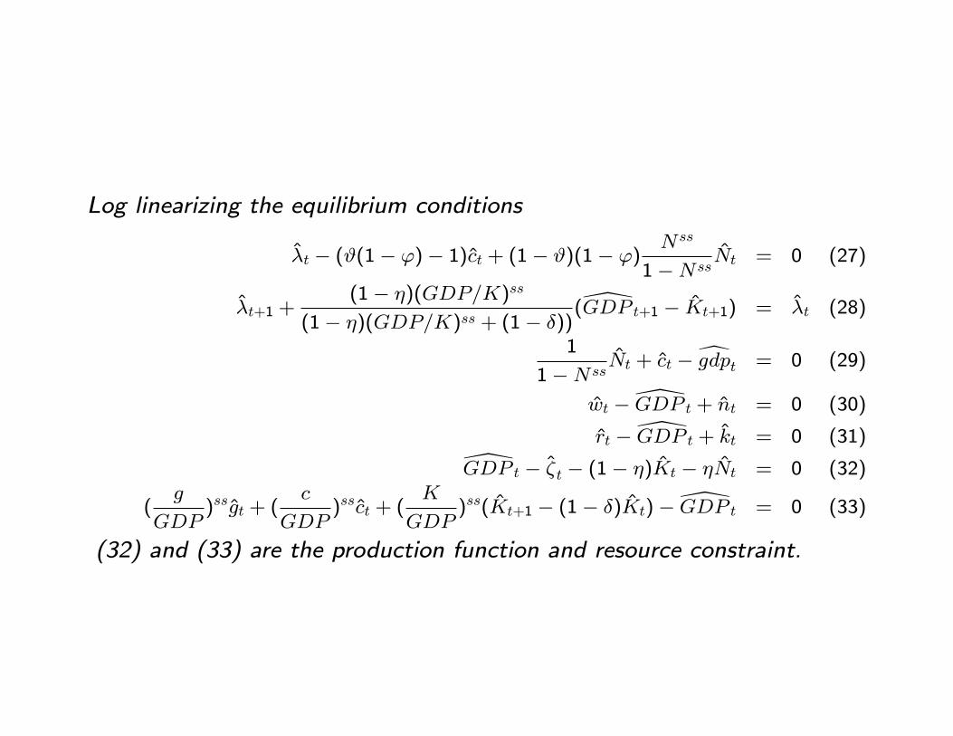
Log linearizing the equilibrium conditions

λt − (ϑ(1− ϕ)− 1)ct + (1− ϑ)(1− ϕ)Nss

1−NssNt = 0 (27)

λt+1 +(1− η)(GDP/K)ss

(1− η)(GDP/K)ss + (1− δ))(GDP t+1 − Kt+1) = λt (28)

1

1−NssNt + ct − gdpt = 0 (29)

wt − GDP t + nt = 0 (30)

rt − GDP t + kt = 0 (31)

GDP t − ζt − (1− η)Kt − ηNt = 0 (32)

(g

GDP)ssgt + (

c

GDP)ssct + (

K

GDP)ss(Kt+1 − (1− δ)Kt)− GDP t = 0 (33)

(32) and (33) are the production function and resource constraint.

Four types of parameters appear in the log-linearized conditions:

i.) Technological parameters (η, δ).

ii) Preference parameters (β, ϕ, ϑ).

iii) Steady state parameters (Nss, ( cGDP )ss, ( K

GDP )ss, ( gGDP )ss).

iv) Parameters of the driving process (ρg, ρz, σ2z, σ

2g).

Question: How do we set a prior for these 13 parameters?

The steady state of the model (using (23)-(26)-(17)) is:

1− ϑϑ

(c

GDP)ss = η

1−Nss

Nss(34)

β[(1− η)(GDP

K)ss + (1− δ)] = 1 (35)

(g

GDP)ss + (

c

GDP)ss + δ(

K

GDP)ss = 1 (36)

GDP

wc= η (37)

K

i= δ (38)

Five equations in 8 parameters!! Need to choose.

For example: (34)-(38) determine (Nss, ( cGDP )ss, ( K

GDP )ss, η, δ) given

(( gGDP )ss, β, ϑ).

Set θ2 = [( gGDP )ss, β, ϑ] and θ1 = [Nss, ( c

GDP )ss, ( KGDP )ss, η, δ]

Then if S1T are steady state relationships, we an use (34)-(38) to construct

a prior distribution for θ1|θ2.

How do we measure uncertainty in S1T?

- Take a rolling window to estimate S1T and use uncertainty of the estimate

to calibrate var(η).

- Bootstrap S1T , etc.

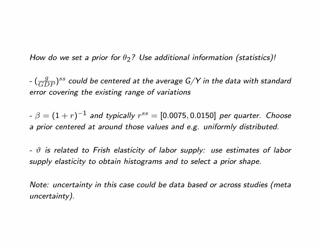
How do we set a prior for θ2? Use additional information (statistics)!

- ( gGDP )ss could be centered at the average G/Y in the data with standard

error covering the existing range of variations

- β = (1 + r)−1 and typically rss = [0.0075, 0.0150] per quarter. Choose

a prior centered at around those values and e.g. uniformly distributed.

- ϑ is related to Frish elasticity of labor supply: use estimates of labor

supply elasticity to obtain histograms and to select a prior shape.

Note: uncertainty in this case could be data based or across studies (meta

uncertainty).

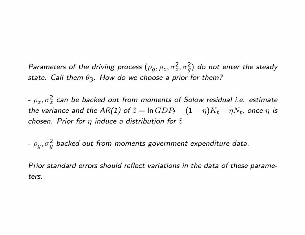
Parameters of the driving process (ρg, ρz, σ2z, σ

2g) do not enter the steady

state. Call them θ3. How do we choose a prior for them?

- ρz, σ2z can be backed out from moments of Solow residual i.e. estimate

the variance and the AR(1) of z = lnGDPt− (1− η)Kt− ηNt, once η is

chosen. Prior for η induce a distribution for z

- ρg, σ2g backed out from moments government expenditure data.

Prior standard errors should reflect variations in the data of these parame-

ters.

- For ϕ (coefficient of relative risk aversion (RRA) is 1 − ϑ(1 − ϕ)) one

has two options:

(a) appeal to existing estimates of RRA. Construct a prior which is con-

sistent with the cross section of estimates (e.g. a χ2(2) would be ok).

(b) select an interesting moment, say var(ct) and use

var(ct) = var(ct(ϕ)|θ1, θ2, θ3) + η (39)

to back out a prior for ϕ.

For some parameters (call them θ5) we have no moments to match but

some micro evidence. Then p(θ5) = π(θ5) could be estimated from the

histogram of the estimates which are available.

In sum, the prior for the parameters is

p(θ) = p(θ1|S1T )p(θ2|S2T )p(θ3|S3T )p(θ4|S4T )

π(θ1)π(θ2)π(θ3)π(θ4)Π(θ5) (40)

- If we had used a different utility function, the prior e.g. for θ1, θ4 would

be different. Prior for different models/parameterizations should be dif-

ferent.

- To use these priors, need a normalizing constant ( (15 is not necessarily a

density). Need a RW metropolis to draw from the priors we have produced.

- Careful about multidimensional ridges: e.g. steady states are 5 equations,

and there are 8 parameters - solution not unique, impossible to invert the

relationship.

- Careful about choosing θ3 and θ4 when there are weak and partial iden-

tification problems.

6.2 Choice of data and estimation

- Does it matter which variables are used to estimate the parameters? Yes.

i) Omitting relevant variables may lead to distortions.

ii) Adding variables may improve the fit, but also increase standard errors

if added variables are irrelevant.

iii) Different variables may identify different parameters (e.g. with aggre-

gate consumption data and no data on who own financial assets may be

very difficult to get estimate the share of rule-of-thumb consumers).

Example 6.3

yt = a1Etyt+1 + a2(it − Etπt+1) + v1t (41)

πt = a3Etπt+1 + a4yt + v2t (42)

it = a5Etπt+1 + v3t (43)

Solution: ytπtit

=

1 0 a2a4 1 a2a40 0 1

v1tv2tv3t

• a1, a3, a5 disappear from the solution.

• Different variables identify different parameters (it identify nothing!!)

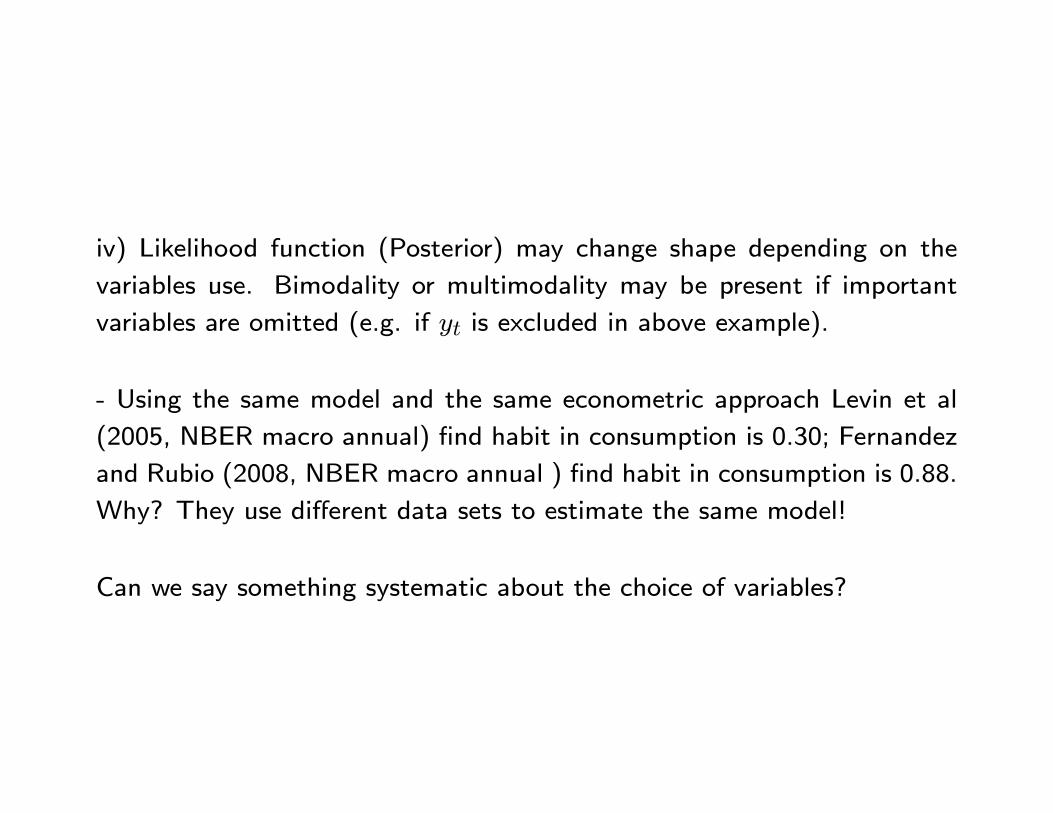
iv) Likelihood function (Posterior) may change shape depending on the

variables use. Bimodality or multimodality may be present if important

variables are omitted (e.g. if yt is excluded in above example).

- Using the same model and the same econometric approach Levin et al

(2005, NBER macro annual) find habit in consumption is 0.30; Fernandez

and Rubio (2008, NBER macro annual ) find habit in consumption is 0.88.

Why? They use different data sets to estimate the same model!

Can we say something systematic about the choice of variables?

Guerron-Quintana (2010); use Smets and Wouters model and different

combinations of observable variables. Finds:

- Internal persistence of the model change if nominal rate, inflation and

real wage are absent.

- Duration of price spells affected by the omission of consumption and real

wage data.

- Responses of inflation, investment, hours and real wage sensitive to the

choice of variables.

- ” Best combination” of variables (use in-sample prediction and out-of-

sample MSE): use Yt, Ct, It, Rt, Ht, πt,W .

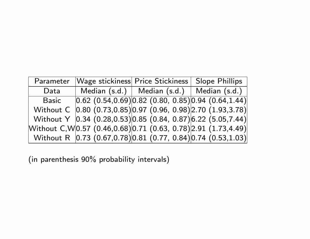
Parameter Wage stickiness Price Stickiness Slope Phillips

Data Median (s.d.) Median (s.d.) Median (s.d.)Basic 0.62 (0.54,0.69)0.82 (0.80, 0.85)0.94 (0.64,1.44)

Without C 0.80 (0.73,0.85)0.97 (0.96, 0.98)2.70 (1.93,3.78)Without Y 0.34 (0.28,0.53)0.85 (0.84, 0.87)6.22 (5.05,7.44)

Without C,W0.57 (0.46,0.68)0.71 (0.63, 0.78)2.91 (1.73,4.49)Without R 0.73 (0.67,0.78)0.81 (0.77, 0.84)0.74 (0.53,1.03)

(in parenthesis 90% probability intervals)

Output recession after an investments specific shock and no C and W.

Canova, Ferroni and Matthes (2012)

• Use statistical criteria to choose the variables in estimation

1) Choose the variables that maximize the identificability of relevant pa-

rameters.

Compute the rank of the derivative of the spectral density of the solution

of the model with respect to the parameters

Komunjer and Ng (2011): have necessary and sufficient conditions for full

identification of the parameters

Choose the combination of observables which gives you a rank as close as

possible to the ideal.

2) Compare the curvature of the convoluted likelihood in the singular and

the non-singular systems in the dimensions of interest.

3) Choose the variables that minimize the information loss going from the

larger scale to the smaller scale system.

Loss of information is measured by

pjt(θ, e

t−1, ut) =L(Wjt|θ, et−1, ut)

L(Zt|θ, et−1, ut)(44)

where L(.|θ, y1t) is the likelihood of Zt,Wjt

Zt = yt + ut (45)

Wjt = Syjt + ut (46)

ut is the convolution error, yt the original set of variables and yjt the j-th

subset of that variables which produce a non-singular system.

• Apply the procedures to choose the best combination of variables in a

SW model driven by only 4 shocks and 7 potential observables.

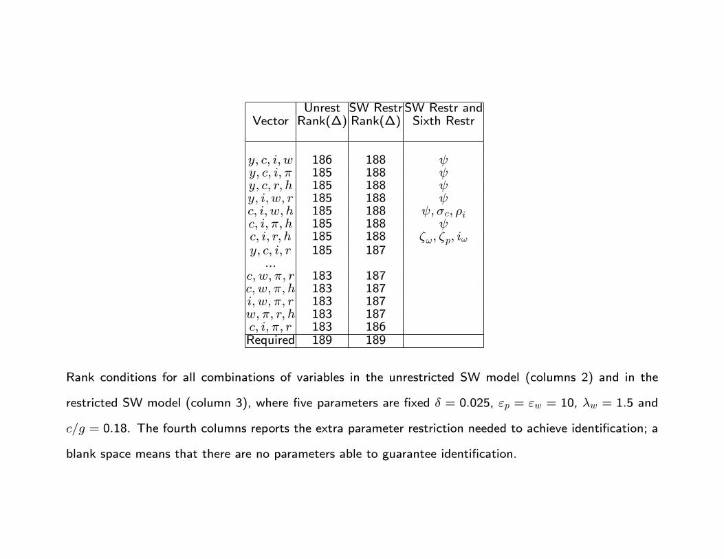
Unrest SW Restr SW Restr andVector Rank(∆) Rank(∆) Sixth Restr

y, c, i, w 186 188 ψy, c, i, π 185 188 ψy, c, r, h 185 188 ψy, i, w, r 185 188 ψc, i, w, h 185 188 ψ, σc, ρic, i, π, h 185 188 ψc, i, r, h 185 188 ζω, ζp, iωy, c, i, r 185 187

...c, w, π, r 183 187c, w, π, h 183 187i, w, π, r 183 187w, π, r, h 183 187c, i, π, r 183 186Required 189 189

Rank conditions for all combinations of variables in the unrestricted SW model (columns 2) and in the

restricted SW model (column 3), where five parameters are fixed δ = 0.025, εp = εw = 10, λw = 1.5 and

c/g = 0.18. The fourth columns reports the extra parameter restriction needed to achieve identification; a

blank space means that there are no parameters able to guarantee identification.

0.65 0.7 0.75

10

0

10

h = 0.710.55 0.6 0.65 0.7 0.75

40

20

0

ξp = 0.650.35 0.4 0.45 0.5 0.55

10

0

10

γp = 0.47

1.6 1.8 2 2.2

10

5

0

5

10

σl = 1.921.8 2 2.2

20

0

20

ρπ = 2.030 0.1 0.2

50

0

50

ρy = 0.08

DGPoptimal

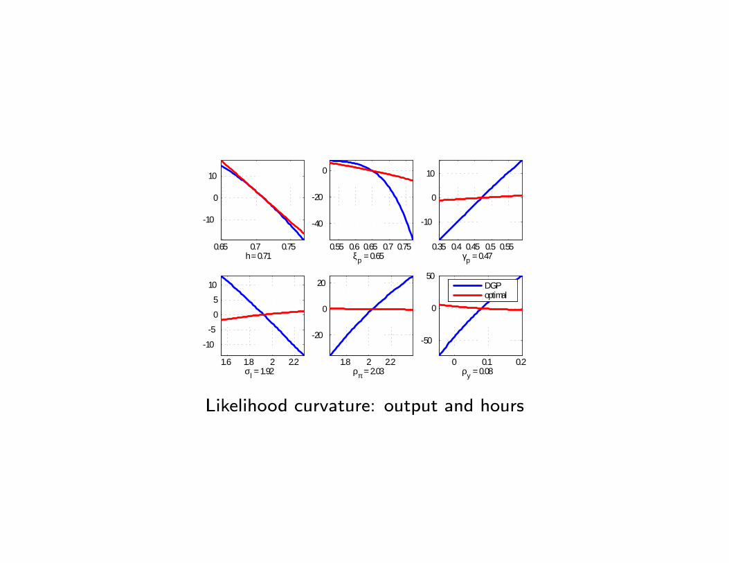
Likelihood curvature: output and hours

0.65 0.7 0.75

10

0

10

h = 0.710.55 0.6 0.65 0.7 0.75

40

20

0

ξp = 0.650.35 0.4 0.45 0.5 0.55

10

0

10

γp = 0.47

1.6 1.8 2 2.210

5

0

5

10

σl = 1.921.8 2 2.2

20

0

20

ρπ = 2.030 0.1 0.2

60

40

20

020

40

ρy = 0.08

DGPoptimal

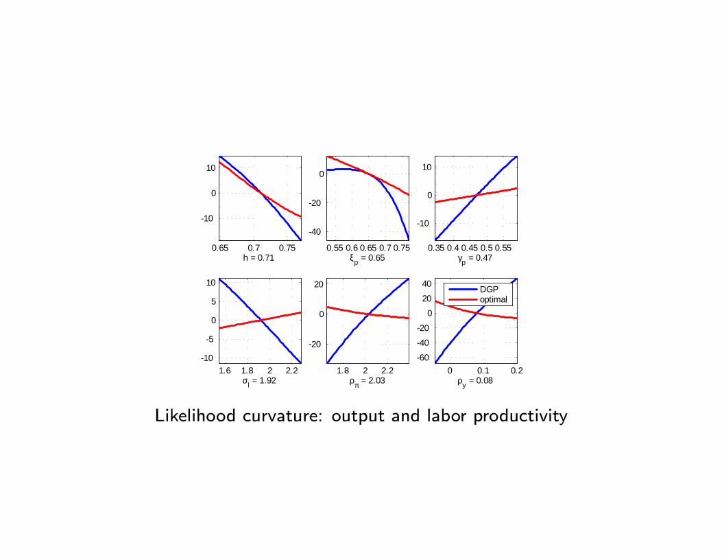
Likelihood curvature: output and labor productivity

Basic T=1500 Σu = 0.01 ∗ IOrder Vector Relative Info Vector Relative info Vector Relative Info

1 (y, c, i, h) 1 (y, c, i, h) 1 (y, c, i, h) 12 (y, c, i, w) 0.89 (y, c, i, w) 0.87 (y, c, i, w) 0.863 (y, c, i, r) 0.52 (y, c, i, r) 0.51 (y, c, i, r) 0.514 (y, c, i, π) 0.5 (y, c, i, π) 0.5 (y, c, i, π) 0.5

Ranking based on the p(θ) statistic. The first two column present the results for the

basic setup, the next six columns the results obtained altering some nuisance parameters.

Relative information is the ratio of the p(θ) statistic relative to the best combination.

How different are good and bad combinations?

- Simulate 200 data points from the model with [at, it, gt, εmt ] and estimate

structural parameters using

(1) Model A: 4 shocks and (y, c, i, w) as observables (best rank analysis).

(2) Model B: 4 shocks and (y, c, i, w) as observables (best information analysis).

(3) Model Z: 4 shocks and (c, i, π, r) as observables(worst rank analysis).

(4) Model C: 4 structural shocks, three measurement errors and (yt, ct, it, wt, π, rt, ht) as

observables.

(5) Model D: 7 structural shocks and (yt, ct, it, wt, π, rt, ht) as observables.

True Model A Model B Model Z Model C Model Dρa 0.95 ( 0.920 , 0.975 ) ( 0.905 , 0.966 ) ( 0.946 , 0.958) ( 0.951 , 0.952 ) ( 0.939 , 0.943 )ρg 0.97 ( 0.930 , 0.969 ) ( 0.930 , 0.972 ) ( 0.601 , 0.856) ( 0.970 , 0.971 ) ( 0.970 , 0.972 )ρi 0.71 ( 0.621 , 0.743 ) ( 0.616 , 0.788 ) ( 0.733 , 0.844) ( 0.681 , 0.684 ) ( 0.655 , 0.669 )ρga 0.51 ( 0.303 , 0.668 ) ( 0.323 , 0.684 ) ( 0.010 ,0.237 ) ( 0.453 , 0.780 ) ( 0.114 , 0.885 )σn 1.92 ( 1.750 , 2.209 ) ( 1.040 , 2.738 ) ( 0.942 , 2.133) ( 1.913 , 1.934 ) ( 1.793 , 1.864 )σc 1.39 ( 1.152 , 1.546 ) ( 1.071 , 1.581 ) ( 1.367 , 1.563) ( 1.468 , 1.496 ) ( 1.417 , 1.444 )h 0.71 ( 0.593 , 0.720 ) ( 0.591 , 0.780 ) ( 0.716 , 0.743 ) (0.699 , 0.701 ) ( 0.732 , 0.746 )ζω 0.73 ( 0.402 , 0.756 ) (0.242, 0.721 ) ( 0.211 ,0.656 ) ( 0.806 , 0.839 )ζp 0.65 ( 0.313 , 0.617 ) ( 0.251 , 0.713 ) ( 0.512 , 0.616 ) ( 0.317 , 0.322 ) ( 0.509 , 0.514 )iω 0.59 ( 0.694 , 0.745 ) ( 0.663 , 0.892 ) ( 0.532 ,0.732 ) ( 0.728 , 0.729 ) ( 0.683 , 0.690 )ip 0.47 ( 0.571 , 0.680 ) ( 0.564 , 0.847 ) ( 0.613 , 0.768 ) ( 0.625 , 0.628 ) ( 0.606 , 0.611 )φp 1.61 ( 1.523 , 1.810 ) ( 1.495 , 1.850 ) ( 1.371 , 1.894 ) ( 1.624 , 1.631 ) ( 1.654 , 1.661 )ϕ 0.26 ( 0.145 , 0.301 ) ( 0.153 , 0.343 ) ( 0.255 , 0.373 ) ( 0.279 , 0.295 ) ( 0.281 , 0.306 )ψ 5.48 ( 3.289 , 7.955 ) ( 3.253 , 7.623 ) ( 2.932 , 7.530 ) ( 11.376 , 13.897 ) ( 4.332 , 5.371 )α 0.2 ( 0.189 , 0.331 ) ( 0.167 , 0.314 ) ( 0.136 , 0.266 ) ( 0.177 , 0.198 ) ( 0.174 , 0.199 )ρπ 2.03 ( 1.309 , 2.547 ) ( 1.277 , 2.642 ) ( 1.718 , 2.573 ) ( 1.868 , 1.980 ) ( 2.119 , 2.188 )ρy 0.08 (0.001 , 0.143 ) ( 0.001 , 0.169 ) ( 0.012 , 0.173) ( 0.124 , 0.162 )ρR 0.87 ( 0.776 , 0.928 ) ( 0.813 , 0.963 ) ( 0.868 , 0.916 ) ( 0.881 , 0.886 )ρ∆y 0.22 ( 0.001 , 0.167 ) (0.010, 0.192 ) ( 0.130 ,0.215 ) (0.235 , 0.244 )σa 0.46 ( 0.261 , 0.575 ) ( 0.382 , 0.460 ) ( 0.420 ,0.677 ) ( 0.357 , 0.422 ) ( 0.386 , 0.455 )σg 0.61 ( 0.551 , 0.655 ) ( 0.551 , 0.657 ) ( 0.071 ,0.113 ) ( 0.536 , 0.629 ) ( 0.585 , 0.688 )σi 0.6 ( 0.569 , 0.771 ) ( 0.532 , 0.756 ) ( 0.503 ,0.663 ) ( 0.561 , 0.660 ) ( 0.693 , 0.819 )σr 0.25 ( 0.100 , 0.259 ) ( 0.078 , 0.286 ) ( 0.225 ,0.267 ) ( 0.226 , 0.265 ) ( 0.222 , 0.261 )

10 20 30 400

0.2

0.4

0.6

y

10 20 30 40

0.2

0.15

0.1

0.05

0

c

10 20 30 40

1

0.5

0i

10 20 30 400.04

0.02

0

0.02

0.04

w

10 20 30 400

0.1

0.2

0.3

0.4

h

10 20 30 400

0.01

0.02

π

10 20 30 400

0.01

0.02

0.03

0.04

r

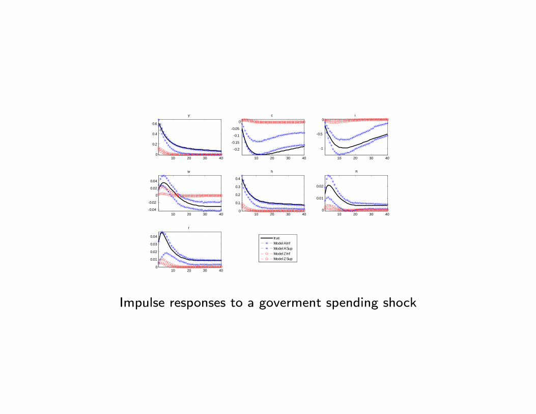
trueModel A InfModel A SupModel Z InfModel Z Sup

Impulse responses to a goverment spending shock

10 20 30 40

0.2

0.4

0.6

y

10 20 30 40

0.1

0.2

0.3

0.4

c

10 20 30 400

0.5

1

1.5

i

10 20 30 40

0.050.1

0.150.2

0.250.3

w

10 20 30 40

0.3

0.2

0.1

0

0.1h

10 20 30 40

0.06

0.04

0.02

0

π

10 20 30 40

0.08

0.06

0.04

0.02

0r

trueModel B InfModel B SupModel C InfModel C Sup

Impulse responses to a technology shock

0 5 10 15 20 25 30 35 400.2

0.15

0.1

0.05

0

0.05

y0 5 10 15 20 25 30 35 40

20

15

10

5

0

5x 10

4

0 5 10 15 20 25 30 35 400.1

0.05

0

0.05

h0 5 10 15 20 25 30 35 40

2

1

0

1x 10

3

0 5 10 15 20 25 30 35 400.1

0

0.1

0.2

π0 5 10 15 20 25 30 35 40

2

0

2

4x 10

3

0 5 10 15 20 25 30 35 400.02

0

0.02

0.04

r0 5 10 15 20 25 30 35 40

5

0

5

10x 10

4

S WE st

Impulse responses to a price markup shock

6.3 Combining DSGE and VARs

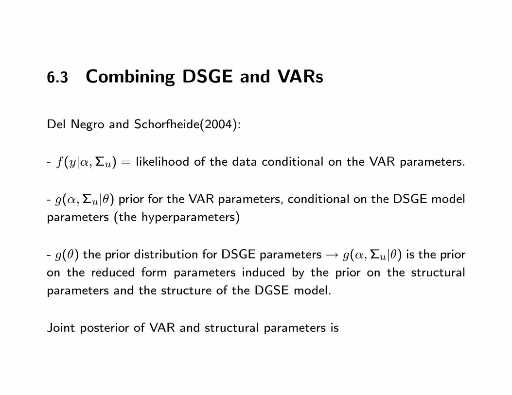
Del Negro and Schorfheide(2004):

- f(y|α,Σu) = likelihood of the data conditional on the VAR parameters.

- g(α,Σu|θ) prior for the VAR parameters, conditional on the DSGE model

parameters (the hyperparameters)

- g(θ) the prior distribution for DSGE parameters→ g(α,Σu|θ) is the prior

on the reduced form parameters induced by the prior on the structural

parameters and the structure of the DGSE model.

Joint posterior of VAR and structural parameters is

f(y|θ) =|T1xs

′(θ)xs(θ) +X ′X|−0.5M |(T1 + T )Σu(θ)|−0.5(T1+T−k)

|τxs′(θ)xs(θ)|−0.5M |T1Σsu(θ)|−0.5(T1−k)

×(2π)−0.5MT2−0.5M(T1+T−k)

∏Mi=1 Γ(0.5 ∗ (T1 + T − k + 1− i))

2−0.5M(T1−k)∏Mi=1 Γ(0.5 ∗ (T1 − k + 1− i))

(47)

T1 = number of simulated observations, Γ is the Gamma function, X

includes all lags of y and the superscript s indicates simulated data.

- Draw θ using an MH algorithm.

- Conditional on θ construct posterior of α (draw α from a Normal-

Wishart).

Estimation algorithm:

1) Draw a candidate θ. Use MCMC to decide if accept or reject.

2) With the draw compute the model induced prior for the VAR parameters.

3) Compute the posterior for the VAR parameters ( analytically if you

have a conjugate structure or via the Gibbs sampler if you do not have

one. Draw from this posterior

4) Repeat steps 1)-3) NL+ L times. Check convergence

5) Repeat 1)-4) for different T1. Choose the T1 that maximizes the mar-

ginal likelihood.

6.4 Practical issues

Log-linear DSGE solution:

y1t = A11(θ)y1t−1 +A13(θ)y3t (48)

y2t = A12(θ)y1t−1 +A23(θ)y3t (49)

where y2t are the control, y1t the states (predetermined and exogenous), y3t the shocks,

θ are the structural parameters and Aij the coefficients of the decision rules.

How to you put DSGE models on the data when:

a) the model implies that the covariance of yt = [y1t, y2t] is singular.

b) the variables are mismeasured relative to the model quantities.

c) have additional information one would like to use.

For a):

• Choose a selection matrix F1 such that dim(x1t) = dim (F1 yt) = dim

(y3t), i.e. throw away model information. Good strategy to follow if some

component of yt are non-observable.

• Explicitly solve out fraction of variables from the model. Format of the

solution is no longer a restricted VAR(1).

• Adds measurement errors to the y2t so that dim(x2t) = dim (F2 yt) =

dim (y3t)+dim (et), where et are measurement errors.

- If the model has two shocks and implications for four variables, we could

add at least two and up to four measurement errors to the model.

Here (1)-(2) are the state equations and the measurement equation is

x2t = F2yt + et (50)

- Need to restrict time series properties of et. Otherwise difficult to distin-

guish dynamics induced by structural shocks and the measurement errors.

i) the measurement error is iid (since θ is identified from the dynamics

induced by the reduced form shocks, if measurement error is iid, θ identified

by the dynamics due to structural shocks).

Ireland (2004): VAR(1) process for the measurement error; identification

problems! Can be used to verify the quality of the model’s approximation

to the data - measurement error captures what is missing from the model to

fit the data (see also Watson (1993)). Useful device when θ is calibrated.

Less useful when θ is estimated.

For b): Recognize that existing measures of theoretical concepts are con-

taminated.

- How do you measure hours? Use establishment survey series? Household

survey series? Employment?

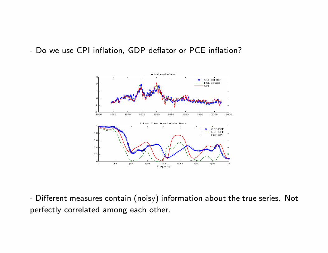
- Do we use CPI inflation, GDP deflator or PCE inflation?

- Different measures contain (noisy) information about the true series. Not

perfectly correlated among each other.

- Use ideas underlying factor models. Let x3t be a k×1 vector of observable

variables and x1t be of dimension N × 1 where dim (N) ¡ dim(k). Then:

x3t = Λ3x1t + ut (51)

where the first row of Λ3 is normalized to 1. Thus:

x3t = Λ3[F1y1t, F1A12(θ)y1t−1 + F1A13(θ)y3t]′ + u3t (52)

= Λ3[F1y1t, F1B(θ)y1t]′ + u3t (53)

so that x3t can be used to recover the vector of states y1t and to estimate

θ

- What is the advantage of this procedure? If only one component of x3t

is used to measure y1t, estimate of θ will probably be noisy.

- By using a vector of information and assuming that the elements of utare idiosyncratic:

i) reduce the noise in the estimate of y1t (the estimated variance of y1t

will be asymptotically of the order 1/k time the variance obtained when

only one indicator is used (see Stock and Watson (2002)).

ii) estimates of θ more precise.

- How different is from factor models?. The DSGE model structure is

imposed in the specification of the law of motion of the states (states have

economic content). In factor models the states are assumed to follow is an

assumed unrestricted time series specification, say an AR(1) or a random

walk and are uninterpretable.

- How do we separately identify the dynamics induced by the structural

shocks and the measurement errors? Since the measurement error is iden-

tified from the cross sectional properties of the variables in x3t, possible

to have structural disturbances and measurement errors to both be serially

correlated of an unknown form.

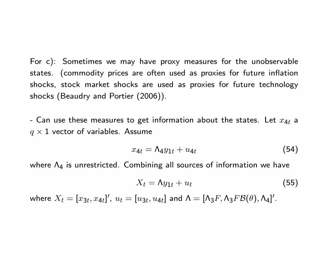
For c): Sometimes we may have proxy measures for the unobservable

states. (commodity prices are often used as proxies for future inflation

shocks, stock market shocks are used as proxies for future technology

shocks (Beaudry and Portier (2006)).

- Can use these measures to get information about the states. Let x4t a

q × 1 vector of variables. Assume

x4t = Λ4y1t + u4t (54)

where Λ4 is unrestricted. Combining all sources of information we have

Xt = Λy1t + ut (55)

where Xt = [x3t, x4t]′, ut = [u3t, u4t] and Λ = [Λ3F,Λ3FB(θ),Λ4]′.

- The fact that we are using the DSGE structure (B depends on θ) im-

poses restrictions on the way the data behaves. (interpret data information

through the lenses of the DSGE model).

- Can still jointly estimate the structural parameters and the unobservable

states of the economy.

6.5 An example

Use a simple three equation New-keynesian model:

xt = Et(xt+1)− 1

φ(it − Etπt+1) + e1t (56)

πt = βEtπt+1 + κxt + e2t (57)

it = ψrit−1 + (1− ψr)(ψππt + ψxxt) + e3t (58)

where β is the discount factor, φ the relative risk aversion coefficient, κthe slope of Phillips curve, (ψr, ψπ, ψx) policy parameters. Here xt is theoutput gap, πt the inflation rate and it the nominal interest rate. Assume

e1t = ρ1e1t−1 + v1t (59)

e2t = ρ2e2t−1 + v2t (60)

e3t = v3t (61)

where ρ1, ρ2 < 1, vjt ∼ (0, σ2j), j = 1, 2, 3.

6.5.1 Contaminated data

- Ambiguities in linking the output gap, the inflation rate and the nominal

interest rate to empirical counterparts. e.g. for the nominal interest rate:

should we use a short term measure or a long term one? for the output

gap, should we use a statistical based measure or a theory based measure?

In the last case, what is the flexible price equilibrium?

The solution of the model can be written as

wt = RR(θ)wt−1 + SS(θ)vt (62)

where wt is a 8 × 1 vector including xt, πt, it, the three shocks and the

expectations of xt and πt and θ = (φ, κ, ψr, ψy, ψπ, ρ1, ρ2, σ1, σ2, σ3).

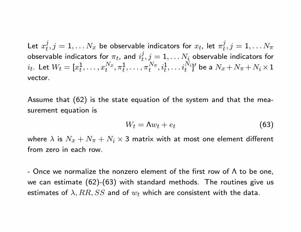
Let xjt , j = 1, . . . Nx be observable indicators for xt, let π

jt , j = 1, . . . Nπ

observable indicators for πt, and ijt , j = 1, . . . Ni observable indicators for

it. Let Wt = [x1t , . . . , x

Nxt , π1

t , . . . , πNπt , i1t , . . . i

Nit ]′ be a Nx+Nπ+Ni×1

vector.

Assume that (62) is the state equation of the system and that the mea-

surement equation is

Wt = Λwt + et (63)

where λ is Nx + Nπ + Ni × 3 matrix with at most one element different

from zero in each row.

- Once we normalize the nonzero element of the first row of Λ to be one,

we can estimate (62)-(63) with standard methods. The routines give us

estimates of λ,RR, SS and of wt which are consistent with the data.

6.5.2 Conjunctoral information

- Suppose we have available measures of future inflation (from surveys,

from forecasting models) or data which may have some information about

future inflation, for example, oil prices, housing prices, etc.

- Want to predict inflation h periods ahead, h = 1, 2, . . ..

Let πjt , j = 1, . . . Nπ be the observable indicators for πt and let Wt =

[xt, it, π1t , . . . , π

Nπt ]′ be a 2 +Nπ × 1 vector.

The measurement equation is:

Wt = Λwt + et (64)

where Λ is 2 +Nπ × 3 matrix, Λ =

1 0 00 1 00 0 10 0 λ1. . . . . . . . .0 0 λNπ

.

- Estimates of the unobservable wt can be obtained with the Kalman

filter. Using estimates of RR(θ) and SS(θ) from the state equation we

can unconditionally predict wt h-steps ahead or predict its path conditional

on a path for vl,t+h.

- Forecast will incorporate information from the model, information from

conjunctural data and from standard data and information about the path

of the shocks. This information will be optimally mixed depending on their

relative precision.

6.6 Dealing with trends

- Most of models available for policy are stationary and cyclical.

- Data is close to non-stationary, has trends and displays breaks.

- How to we match models to the data?

a) Detrend actual data. Model is a representation for detrended data stan-

dard approach. Problem: which detrended data is the model representing?

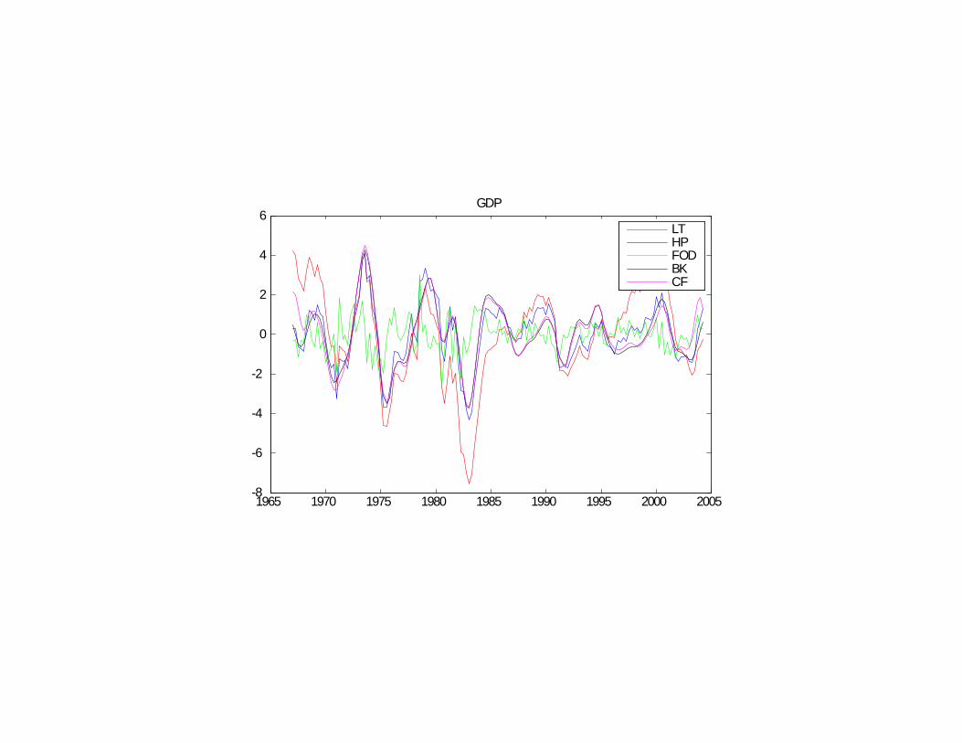
1965 1970 1975 1980 1985 1990 1995 2000 20058

6

4

2

0

2

4

6GDP

LTHPFODBKCF

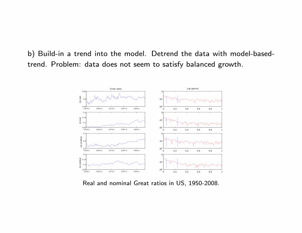
b) Build-in a trend into the model. Detrend the data with model-based-

trend. Problem: data does not seem to satisfy balanced growth.

1950 :1 1962 :4 1975 :1 1987 :2 2000 :10 .55

0 .6

0 .65Great ratios

c/y

real

1950 :1 1962 :2 1975 :1 1987 :2 2000 :10 .05

0 .1

0 .15

0 .2

i/y re

al

1950 :1 1962 :2 1975 :1 1987 :2 2000 :10 .5

0 .6

0 .7

c/y

nom

inal

1950 :1 1962 :2 1975 :1 1987 :2 2000 :10 .05

0 .1

0 .15

0 .2

i/y n

omin

al

0 0.2 0.4 0.6 0.8 120

10

0Log spectra

0 0.2 0.4 0.6 0.8 120

10

0

0 0.2 0.4 0.6 0.8 120

10

0

0 0.2 0.4 0.6 0.8 120

10

0

Real and nominal Great ratios in US, 1950-2008.

c) Use transformation of the data which allow you to estimate jointly cycle

and the parameters trend (see e.g. growth rates in Smets and Wouter

2007). Problem: hard to fit models to quarterly growth rates

- General problem: statistical definition of cycles different than economic

definition. All statistical approaches are biased even in large samples.

0 0.5 1 1.5 2 2.5 3 3.50

1000

2000

3000

4000

5000

6000

7000

8000

9000

10000Ideal Situation

datacycle 1

Ideal case

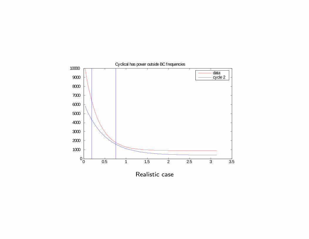
0 0.5 1 1.5 2 2.5 3 3.50

1000

2000

3000

4000

5000

6000

7000

8000

9000

10000Cyclical has power outside BC frequencies

datacycle 2

Realistic case

0 0.5 1 1.5 2 2.5 3 3.50

1000

2000

3000

4000

5000

6000

7000

8000

9000

10000Noncyclical has power at BC frequencies

datacycle 3

General case

- In developing countries most of cyclical fluctuations driven by trends

(Aguiar and Gopinath (2007)).

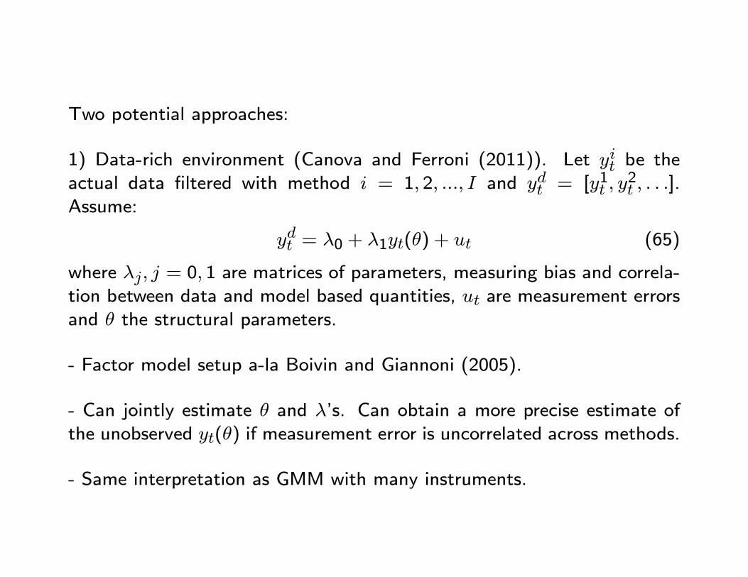
Two potential approaches:

1) Data-rich environment (Canova and Ferroni (2011)). Let yit be theactual data filtered with method i = 1, 2, ..., I and ydt = [y1

t , y2t , . . .].

Assume:

ydt = λ0 + λ1yt(θ) + ut (65)

where λj, j = 0, 1 are matrices of parameters, measuring bias and correla-tion between data and model based quantities, ut are measurement errorsand θ the structural parameters.

- Factor model setup a-la Boivin and Giannoni (2005).

- Can jointly estimate θ and λ’s. Can obtain a more precise estimate ofthe unobserved yt(θ) if measurement error is uncorrelated across methods.

- Same interpretation as GMM with many instruments.

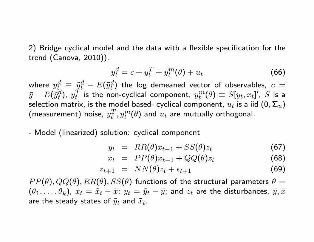
2) Bridge cyclical model and the data with a flexible specification for thetrend (Canova, 2010)).

ydt = c+ yTt + ymt (θ) + ut (66)

where ydt ≡ ydt − E(ydt ) the log demeaned vector of observables, c =y − E(ydt ), yTt is the non-cyclical component, ymt (θ) ≡ S[yt, xt]

′, S is aselection matrix, is the model based- cyclical component, ut is a iid (0,Σu)(measurement) noise, yTt , y

mt (θ) and ut are mutually orthogonal.

- Model (linearized) solution: cyclical component

yt = RR(θ)xt−1 + SS(θ)zt (67)

xt = PP (θ)xt−1 +QQ(θ)zt (68)

zt+1 = NN(θ)zt + εt+1 (69)

PP (θ), QQ(θ), RR(θ), SS(θ) functions of the structural parameters θ =(θ1, . . . , θk), xt = xt − x; yt = yt − y; and zt are the disturbances, y, xare the steady states of yt and xt.

- Non cyclical component

yTt = yTt−1 + yt−1 + et et ∼ iid (0,Σ2e) (70)

yt = yt−1 + vt vt ∼ iid (0,Σ2v) (71)

Σ2v > 0 and Σ2

e = 0, yTt is a vector of I(2) processes.

Σ2v = 0, and Σ2

e > 0, yTt is a vector of I(1) processes.

Σ2v = Σ2

e = 0, yTt is deterministic.

Σ2v > 0 and Σ2

e > 0 and σ2vσ

2e is large, ytt is ”smooth” and nonlinear ( as

in HP).

- Jointly estimate structural θ and non-structural parameters.

Example 6.4 The log linearized equilibrium conditions of basic NK model are:

λt = χt −σc

1− h(yt − hyt−1) (72)

yt = zt + (1− α)nt (73)

wt = −λt + σnnt (74)

rt = ρrrt−1 + (1− ρr)(ρππt + ρyyt) + vt (75)

λt = Et(λt+1 + rt − πt+1) (76)

πt = kp(wt + nt − yt + µt) + βEtπt+1 (77)

zt = ρzzt−1 + ιzt (78)

where kp =(1−βζp)(1−ζp)

ζp

1−α1−α+εα

, λ is the Lagrangian on the consumer budget constraint,

zt is a technology shock, χt a preference shock, vt is an iid monetary policy shock and εt

an iid markup shock.

Filter LT HP FOD BP FlexibleParameter True Median (s.d.)Median (s.d.)Median (s.d.)Median(s.d.)Median(s.d.)

σc 3.00 2.08 (0.11) 2.08 (0.14) 1.89 (0.14) 2.13 (0.12) 3.68( 0.40)σn 0.70 1.72 (0.09) 1.36 (0.07) 1.24 (0.06) 1.58 (0.08) 0.54( 0.14)h 0.70 0.67 (0.02) 0.58 (0.03) 0.36 (0.03) 0.66 (0.02) 0.55( 0.04)α 0.60 0.28 (0.03) 0.15 (0.02) 0.14 (0.02) 0.17 (0.02) 0.19( 0.03)ε 7.00 3.19 (0.11) 5.13 (0.19) 3.76 (0.18) 3.80 (0.13) 6.19( 0.07)ρr 0.20 0.54 (0.03) 0.77 (0.03) 0.72 (0.04) 0.53 (0.03) 0.16( 0.04)ρπ 1.20 1.69 (0.08) 1.65 (0.06) 1.65 (0.07) 1.63 (0.10) 0.30( 0.04)ρy 0.05 -0.14 (0.04) 0.45 (0.04) 0.63 (0.06) 0.40 (0.04) 0.07( 0.03)ζp 0.80 0.85 (0.03) 0.91 (0.03) 0.93 (0.03) 0.90 (0.03) 0.78( 0.04)ρχ 0.50 1.00 (0.03) 0.96 (0.03) 0.96 (0.03) 0.95 (0.03) 0.53( 0.02)ρz 0.80 0.84 (0.03) 0.96 (0.03) 0.97 (0.03) 0.96 (0.03) 0.71( 0.03)σχ 1.12 0.11 (0.02) 0.17 (0.02) 0.21 (0.03) 0.14 (0.02) 1.29( 0.01)σz 0.51 0.07 (0.01) 0.09 (0.01) 0.09 (0.01) 0.07 (0.01) 0.72( 0.02)σmp 0.10 0.05 (0.01) 0.05 (0.01) 0.05 (0.01) 0.05 (0.01) 0.22( 0.004)σµ 20.60 6.30 (0.50) 16.75 (0.62) 22.75 (0.83) 14.40 (0.58) 15.88( 0.06)σncχ 3.21

σncχ is the standard deviation of the non-cyclical component. Parameters Estimates using

different filters, small variance of non-cyclical shock

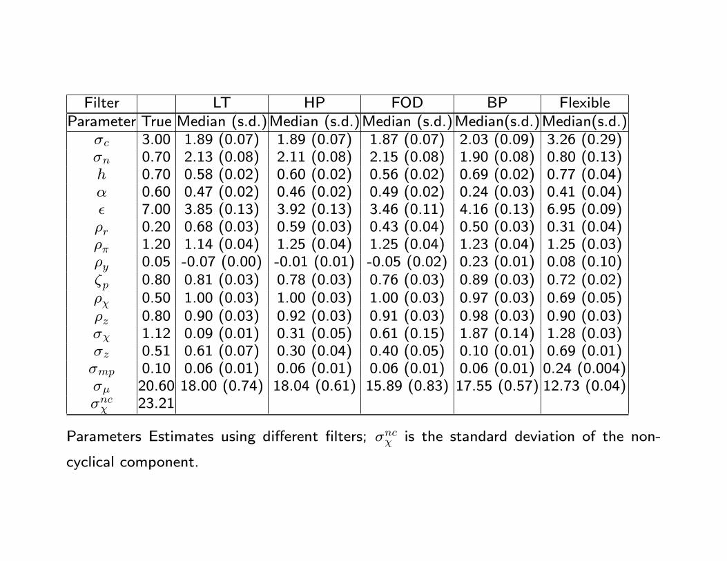
Filter LT HP FOD BP FlexibleParameter True Median (s.d.)Median (s.d.)Median (s.d.)Median(s.d.)Median(s.d.)

σc 3.00 1.89 (0.07) 1.89 (0.07) 1.87 (0.07) 2.03 (0.09) 3.26 (0.29)σn 0.70 2.13 (0.08) 2.11 (0.08) 2.15 (0.08) 1.90 (0.08) 0.80 (0.13)h 0.70 0.58 (0.02) 0.60 (0.02) 0.56 (0.02) 0.69 (0.02) 0.77 (0.04)α 0.60 0.47 (0.02) 0.46 (0.02) 0.49 (0.02) 0.24 (0.03) 0.41 (0.04)ε 7.00 3.85 (0.13) 3.92 (0.13) 3.46 (0.11) 4.16 (0.13) 6.95 (0.09)ρr 0.20 0.68 (0.03) 0.59 (0.03) 0.43 (0.04) 0.50 (0.03) 0.31 (0.04)ρπ 1.20 1.14 (0.04) 1.25 (0.04) 1.25 (0.04) 1.23 (0.04) 1.25 (0.03)ρy 0.05 -0.07 (0.00) -0.01 (0.01) -0.05 (0.02) 0.23 (0.01) 0.08 (0.10)ζp 0.80 0.81 (0.03) 0.78 (0.03) 0.76 (0.03) 0.89 (0.03) 0.72 (0.02)ρχ 0.50 1.00 (0.03) 1.00 (0.03) 1.00 (0.03) 0.97 (0.03) 0.69 (0.05)ρz 0.80 0.90 (0.03) 0.92 (0.03) 0.91 (0.03) 0.98 (0.03) 0.90 (0.03)σχ 1.12 0.09 (0.01) 0.31 (0.05) 0.61 (0.15) 1.87 (0.14) 1.28 (0.03)σz 0.51 0.61 (0.07) 0.30 (0.04) 0.40 (0.05) 0.10 (0.01) 0.69 (0.01)σmp 0.10 0.06 (0.01) 0.06 (0.01) 0.06 (0.01) 0.06 (0.01) 0.24 (0.004)σµ 20.60 18.00 (0.74) 18.04 (0.61) 15.89 (0.83) 17.55 (0.57) 12.73 (0.04)σncχ 23.21

Parameters Estimates using different filters; σncχ is the standard deviation of the non-

cyclical component.

Why are estimates distorted?

- Posterior proportional to likelihood times prior.

- Log-likelihood of the parameters (see Hansen and Sargent (1993))

L(θ|yt) = A1(θ) +A2(θ) +A3(θ)

A1(θ) =1

π

∑ωj

log detGθ(ωj)

A2(θ) =1

π

∑ωj

trace [Gθ(ωj)]−1F (ωj)

A3(θ) = (E(y)− µ(θ))Gθ(ω0)−1(E(y)− µ(θ))

where ωj = πjT , j = 0, 1, . . . , T − 1,, Gθ(ωj) is the model based spectral

density matrix of yt, µ(θ) the model based mean of yt, F (ωj) is the data

based spectral density of yt and E(y) the unconditional mean of the data.

- first term: sum of the one-step ahead forecast error matrix across fre-

quencies;

- the second a penalty function, emphasizing deviations of the model-based

from the data-based spectral density at various frequencies.

- the third another penalty function, weighting deviations of model-based

from data-based means, with the spectral density matrix of the model at

frequency zero.

- Suppose that the actual data is filtered so that frequency zero is elimi-

nated and low frequencies deemphasized. Then

L(θ|yt) = A1(θ) +A2(θ)∗

A2(θ)∗ =1

π

∑ωj

trace [Gθ(ωj)]−1F (ωj)∗

where F (ωj)∗ = F (ωj)Iω and Iω is an indicator function.

Suppose that Iω = I[ω1,ω2], an indicator function for the business cycle

frequencies, as in an ideal BP filter.

The penalty A2(θ)∗ matters only at these frequencies.

Since A2(θ)∗ and A1(θ) enter additively in the log-likelihood function,

there are two types of biases in θ.

- estimates Fθ(ωj)∗ only approximately capture the features of F (ωj)

∗

at the required frequencies - the sample version of A2(θ)∗ has a smaller

values at business cycle frequencies and a nonzero value at non-business

cycle ones.

- To reduce the contribution of the penalty function to the log-likelihood,

parameters are adjusted to make [Gθ(ωj)] close to F (ωj)∗ at those fre-

quencies where F (ωj)∗ is not zero. This is done by allowing fitting errors in

A1(θ) large at frequencies F (ωj)∗ is zero - in particular the low frequencies.

Conclusions:

1) The volatility of the structural shocks will be overestimated - this makes

[Gθ(ωj)] close to F (ωj)∗ at the relevant frequencies.

2) Their persistence underestimated - this makes Gθ(ωj) small and the

fitting error large at low frequencies.

Estimated economy very different from the true one: agents’ decision rules

are altered.

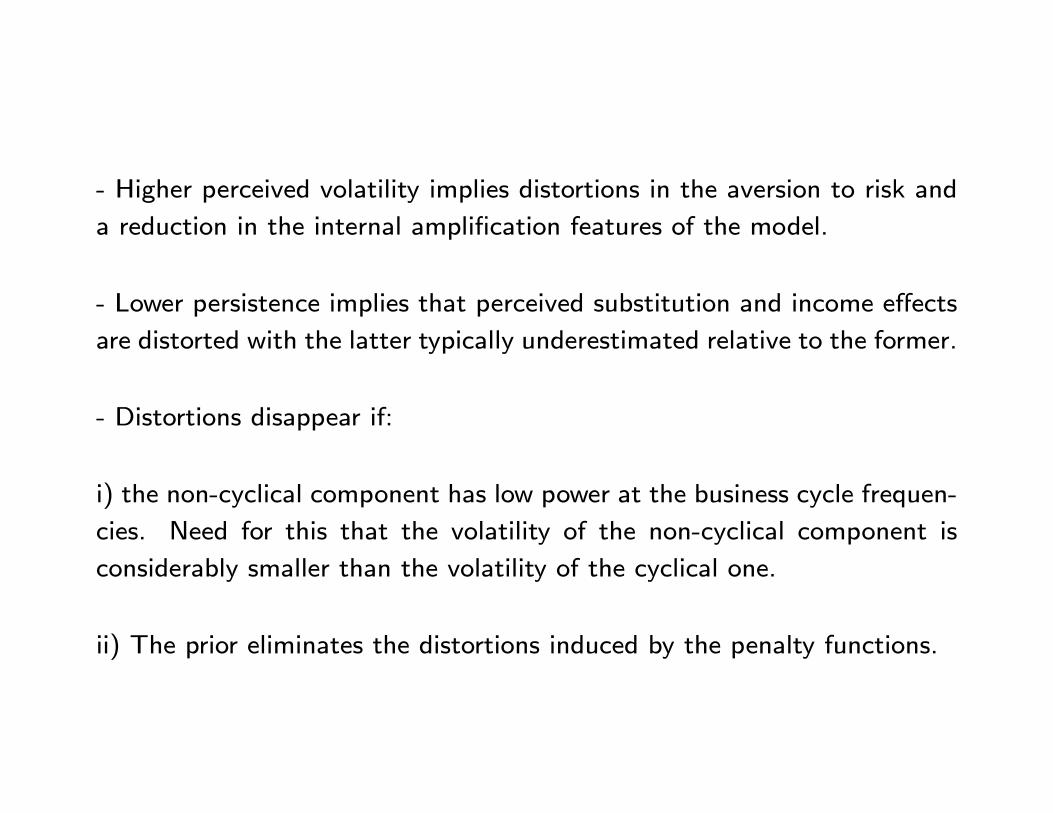
- Higher perceived volatility implies distortions in the aversion to risk and

a reduction in the internal amplification features of the model.

- Lower persistence implies that perceived substitution and income effects

are distorted with the latter typically underestimated relative to the former.

- Distortions disappear if:

i) the non-cyclical component has low power at the business cycle frequen-

cies. Need for this that the volatility of the non-cyclical component is

considerably smaller than the volatility of the cyclical one.

ii) The prior eliminates the distortions induced by the penalty functions.

Question: What if we fit the filtered version of the model to the filtered

data? (CKM (2008))

- Log-likelihood=A1(θ)∗ = 1π

∑ωj log detGθ(ωj)Iω+A2(θ). Suppose that

Iω = I[ω1,ω2].

- A1(θ)∗ matters only at business cycle frequencies while the penalty func-

tion is present at all frequencies.

- If the penalty is more important in the low frequencies (typical case)

parameters adjusted to make [Gθ(ωj)] close to F (ωj) at these frequencies.

-Procedure implies that the model is fitted to the low frequencies com-

ponents of the data!!!

i) Volatility of the shocks will be generally underestimated.

ii) Persistence overestimated.

iii) Since less noise is perceived, decision rules will imply a higher degree

of predictability of simulated time series.

iv) Perceived substitution and income effects are distorted with the latter

overestimated.

How can we avoid distortions?

- Build models with non-cyclical components (difficult).

- Use filters which flexibly adapt, see Gorodnichenko and Ng (2007) and

Eklund, et al. (2008).

- ?

Advantages of suggested approach:

• No need to take a stand on the properties of the non-cyclical component

and on the choice of filter to tone down its importance - specification errors

and biases limited.

• Estimated cyclical component not localized at particular frequencies of

the spectrum.

- Cyclical, non-cyclical and measurement error fluctuations driven by dif-

ferent and orthogonal shocks. But model is observationally equivalent to

one where cyclical and non-cyclical are correlated.

An experiment, again

- Simulate data from the model, assuming that the preference shock has

two components: a nonstationary one and a stationary one (the properties

of the other three shocks are unchanged).

- Variance of the non-cyclical shock is large or small relative to the variance

of the other shocks.

- Use same Bayesian approach, same prior for structural parameters and

gamma priors with large variance for non-structural ones.

- Compute the model-based cyclical component; calculate the autocorrela-

tion function and the log spectrum of output after passing it through LT,

HP, FOD, BP.

Small variance Large varianceTrue Median (s.e) True Median (s.e)

σc 3.00 3.68 (0.40) 3.00 3.26 ( 0.29)σn 0.70 0.54 (0.14) 0.70 0.80 ( 0.13)h 0.70 0.55 (0.04) 0.70 0.77 ( 0.04)α 0.60 0.19 (0.03) 0.60 0.41 ( 0.04)ε 7.00 6.19 (0.07) 7.00 6.95 ( 0.09)ρr 0.20 0.16 (0.04) 0.24 0.31 ( 0.04)ρπ 1.30 1.30 (0.04) 1.30 1.25 ( 0.03)ρy 0.05 0.07 (0.03) 0.05 0.08 ( 0.10)ζp 0.80 0.78 (0.04) 0.80 0.72 ( 0.02)ρχ 0.50 0.53 (0.04) 0.50 0.69 ( 0.05)ρz 0.80 0.71 (0.03) 0.80 0.90 ( 0.03)σχ 0.011 0.012 (0.0003)0.011 0.012 ( 0.0003)σz 0.005 0.006 (0.0001)0.005 0.007 ( 0.0001)σmp0.001 0.002 (0.0004)0.001 0.002 (0.0004)σµ 0.206 0.158 (0.0006)0.206 0.1273 (0.0004)σncχ 0.02 0.23

Parameters estimates using flexible specification. σncχ is the standard error of the shock

to the non-cyclical component.

- Estimates of the structural parameters are roughly unchanged in two

specifications.

- Estimates are precise but the median is not the true value (problem bigger

for α or σn which are only weakly identified).

- The relative magnitude of the various shocks and their persistence is well

estimated. Hence, true and estimated decision rules are similar.

0 0.5 120

15

10

5HP filtered data

True Estimated

0 0.5 1504030

2010

0BP filtered data

True Estimated

0 0.5 120

15

10

5

Fractions of pi

LT data

True Estimated

0 0.5 118

16

14

12

10

Fractions of pi

FOD data

True Estimated

Model based cyclical output spectra, true and estimated, different

filtering. Vertical bars indicate the frequencies where cycles with 8-32

quarters periodicities are located

0 20 40 600.5

0

0.5

1HP filtered data

True Estimated

0 20 40 601

0.5

0

0.5

1HP filtered data

True Estimated

0 20 40 600.5

0

0.5

1LT data

True Estimated

0 20 40 600.5

0

0.5

1FOD data

True Estimated

Autocorrelation function of filtered cyclical component, true and

estimated

5 10 150

0.1

0.2Preference

y t

5 10 150

0.1

0.2Technology

5 10 150.2

0.1

0Monetary Policy

5 10 152

1

0x 10 3Markup

5 10 150.2

0

0.2

ω t

5 10 152

1

0

5 10 152

1

0

5 10 150.04

0.02

0

5 10 150

0.01

0.02

π t

5 10 150.4

0.2

0

5 10 150.1

0.05

0

5 10 150.02

0

0.02

5 10 150

0.02

0.04

r t

5 10 150.4

0.2

0

5 10 151

0

1

5 10 150.02

0

0.02

True Estimated

Model based IRF, true and estimated.

- The true and estimated log spectrum and the autocorrelation function of

the model-based cyclical component close, regardless of the filter.

- Both true and estimate cyclical components have power at all frequencies

of the spectrum.

Actual data: do we get a different story?

1 0.5 0 0.5 10

1

2

3

4

5

6LT

0.7 0.6 0.5 0.4 0.3 0.2 0.1 00

2

4

6

8HP

0.8 0.6 0.4 0.2 0 0.20

1

2

3

4Flexible

0.1 0.05 0 0.05 0.10

5

10

15

20

25

30

35Flexible, inflation target

Sample 19641979 Sample 19842005

Figure 5: Posterior distributions of the policy activism parameter, samples

1964:1-1979:4 and 1984:1-2007:4. LT refers to linearly detrended data, HP to Hodrick

and Prescott filtered data and Flexible to the approach the paper suggests

LT FOD FlexibleOutput Inflation Output Inflation Output Inflation

TFP shocks 0.01 0.04 0.00 0.01 0.01 0.19Gov. expenditure shocks 0.00 0.00 0.00 0.00 0.00 0.02

Investment shocks 0.08 0.00 0.00 0.00 0.00 0.05Monetary policy shocks 0.01 0.00 0.00 0.00 0.00 0.01

Price markup shocks 0.75(*) 0.88(*) 0.91(*) 0.90(*) 0.00 0.21Wage markup shocks 0.00 0.01 0.08 0.08 0.03 0.49(*)

Preference shocks 0.11 0.04 0.00 0.00 0.94(*) 0.00

Variance decomposition at the 5 years horizon. Estimates are obtained using the median

of the posterior of the parameters. A (*) indicates that the 68 percent highest credible

set is entirely above 0.10. The model and the data set are the same as in Smets Wouters

(2007). LT refers to linearly detrended data, FOD to growth rates and Flexible to the

approach this paper suggests.

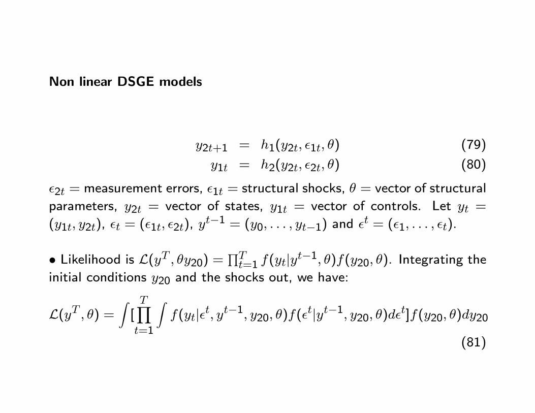
Non linear DSGE models

y2t+1 = h1(y2t, ε1t, θ) (79)

y1t = h2(y2t, ε2t, θ) (80)

ε2t = measurement errors, ε1t = structural shocks, θ = vector of structural

parameters, y2t = vector of states, y1t = vector of controls. Let yt =

(y1t, y2t), εt = (ε1t, ε2t), yt−1 = (y0, . . . , yt−1) and εt = (ε1, . . . , εt).

• Likelihood is L(yT , θy20) =∏Tt=1 f(yt|yt−1, θ)f(y20, θ). Integrating the

initial conditions y20 and the shocks out, we have:

L(yT , θ) =∫

[T∏t=1

∫f(yt|εt, yt−1, y20, θ)f(εt|yt−1, y20, θ)dεt]f(y20, θ)dy20

(81)

(81) is intractable.

• If we have L draws for y20 from f(y20, θ) and L draws for εt|t−1,l,

l = 1, . . . , L, t = 1, . . . , T , from f(εt|yt−1, y20, θ) approximate (81) with

L(yT , θ) =1

L[T∏t=1

1

L

∑l

f(yt|εt|t−1,l, yt−1, yl20, θ)] (82)

Drawing from f(y20, θ) is simple; drawing from f(εt|yt−1, y20, θ) compli-

cated. Fernandez-Villaverde and Rubio-Ramirez (2004):

use f(εt−1|yt−1, y20, θ) as importance sampling for f(εt|yt−1, y20, θ):

- Draw yl20 from f(y20, θ). Draw εt|t−1,l L times from f(εt|yt−1, yl20, θ) =f(εt−1|yt−1, yl20, θ)f(εt|θ).

- Construct IRlt =f(yt|εt|t−1,l,yt−1,yl20,θ)∑Ll=1 f(yt|εt|t−1,l,yt−1,yl20,θ)

and assign it to each draw

εt|t−1,l.

- Resample from εt|t−1,lLl=1with probabilities equal to IRlt.

- Repeat above steps for every t = 1, 2, . . . , T .

Step 3) is crucial, if omitted, only one particle will asymptotically remainand the integral in (81) diverges as T →∞.

• Algorithm is computationally demanding. You need a MC within a MC.Fernandez-Villaverde and Rubio-Ramirez (2004): some improvements overlinear specifications.

Bayesian Methods for DSGE models - European...

Documents

Transcript of Bayesian Methods for DSGE models - European...