Bayesian Learning for Safe High-SpeedNavigation in Unknown Environments

Charles Richter, William Vega-Brown, and Nicholas Roy

In Proceedings of the International Symposium on Robotics Research (ISRR 2015).

Abstract In this work, we develop a planner for high-speed navigation in unknownenvironments, for example reaching a goal in an unknown building in minimumtime, or flying as fast as possible through a forest. This planning task is challengingbecause the distribution over possible maps, which is needed to estimate the feasibil-ity and cost of trajectories, is unknown and extremely hard to model for real-worldenvironments. At the same time, the worst-case assumptions that a receding-horizonplanner might make about the unknown regions of the map may be overly conserva-tive, and may limit performance. Therefore, robots must make accurate predictionsabout what will happen beyond the map frontiers to navigate as fast as possible. Toreason about uncertainty in the map, we model this problem as a POMDP and dis-cuss why it is so difficult given that we have no accurate probability distribution overreal-world environments. We then present a novel method of predicting collisionprobabilities based on training data, which compensates for the missing environ-ment distribution and provides an approximate solution to the POMDP. Extendingour previous work, the principal result of this paper is that by using a Bayesiannon-parametric learning algorithm that encodes formal safety constraints as a priorover collision probabilities, our planner seamlessly reverts to safe behavior whenit encounters a novel environment for which it has no relevant training data. Thisstrategy generalizes our method across all environment types, including those forwhich we have training data as well as those for which we do not. In familiar en-vironment types with dense training data, we show an 80% speed improvementcompared to a planner that is constrained to guarantee safety. In experiments, ourplanner has reached over 8 m/s in unknown cluttered indoor spaces. Video of our ex-perimental demonstration is available at http://groups.csail.mit.edu/rrg/bayesian_learning_high_speed_nav.

1 Introduction

A common planning strategy in unknown environments is the receding-horizon ap-proach: plan a partial trajectory given the current (partial) map knowledge, and be-gin to execute it while re-planning. By repeatedly re-planning, the robot can react tonew map information as it is perceived. However, avoiding collision in a receding-

Charles Richter, William Vega-Brown, and Nicholas RoyMassachusetts Institute of Technology, 77 Massachusetts Ave, Cambridge, MA 02139, e-mail:car,wrvb,nickroy@mit.edu

1

2 Charles Richter, William Vega-Brown, and Nicholas Roy

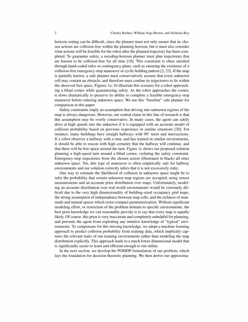
horizon setting can be difficult, since the planner must not only ensure that its cho-sen actions are collision-free within the planning horizon, but it must also considerwhat actions will be feasible for the robot after the planned trajectory has been com-pleted. To guarantee safety, a receding-horizon planner must plan trajectories thatare known to be collision-free for all time [10]. This constraint is often satisfiedthrough hand-coded rules or contingency plans, such as ensuring the existence of acollision-free emergency-stop maneuver or cyclic holding pattern [2, 23]. If the mapis partially known, a safe planner must conservatively assume that every unknowncell may contain an obstacle, and therefore must confine its trajectories to lie withinthe observed free space. Figures 1a–1b illustrate this scenario for a robot approach-ing a blind corner while guaranteeing safety. As the robot approaches the corner,it slows dramatically to preserve its ability to complete a feasible emergency-stopmaneuver before entering unknown space. We use this “baseline” safe planner forcomparison in this paper.

Safety constraints imply an assumption that driving into unknown regions of themap is always dangerous. However, our central claim in this line of research is thatthis assumption may be overly conservative. In many cases, the agent can safelydrive at high speeds into the unknown if it is equipped with an accurate model ofcollision probability based on previous experience in similar situations [20]. Forinstance, many buildings have straight hallways with 90 turns and intersections.If a robot observes a hallway with a turn, and has trained in similar environments,it should be able to reason with high certainty that the hallway will continue, andthat there will be free space around the turn. Figure 1c shows our proposed solutionplanning a high-speed turn around a blind corner, violating the safety constraint.Emergency-stop trajectories from the chosen action (illustrated in black) all enterunknown space. Yet, this type of maneuver is often empirically safe for hallwayenvironments and our solution correctly infers that it is not excessively risky.

One way to estimate the likelihood of collision in unknown space might be toinfer the probability that certain unknown map regions are occupied, using sensormeasurements and an accurate prior distribution over maps. Unfortunately, model-ing an accurate distribution over real-world environments would be extremely dif-ficult due to the very high dimensionality of building-sized occupancy grid maps,the strong assumption of independence between map cells, and the richness of man-made and natural spaces which resist compact parameterization. Without significantmodeling effort, or restriction of the problem domain to specific environments, thebest prior knowledge we can reasonably provide is to say that every map is equallylikely. Of course, this prior is very inaccurate and completely unhelpful for planning,and prevents the agent from exploiting any intuitive knowledge of “typical” envi-ronments. To compensate for this missing knowledge, we adopt a machine learningapproach to predict collision probability from training data, which implicitly cap-tures the relevant traits of our training environments rather than modeling the mapdistribution explicitly. This approach leads to a much lower-dimensional model thatis significantly easier to learn and efficient enough to run online.

In the next section, we develop the POMDP formulation of our problem, whichlays the foundation for decision theoretic planning. We then derive our approxima-

Bayesian Learning for Safe High-Speed Navigation in Unknown Environments 3

(a) (b) (c)

Fig. 1: Actions chosen for a robot approaching a blind corner while guaranteeingsafety (a)–(b). Chosen trajectories are drawn in blue, and feasible emergency-stopmaneuvers are drawn in red. Emergency-stop actions that would cause the robot tocollide with obstacles or unknown cells are drawn in black. The safety constraintrequires the robot to slow from 4 m/s in (a) to 1 m/s in (b) to preserve the ability tostop within known free space. In (c), our solution plans a 6 m/s turn, which commitsthe robot to entering the unknown, but the planner’s experience predicts a low riskof collision. The light gray region shows the hallway of the true hidden map.

tions to the POMDP to make the problem tractable, which give rise to our learnedmodel of collision probability. Then, we discuss how we learn that model and howwe encode safety constraints as a prior over collision probability to help our plannerremain safe in novel environments for which it has no relevant training data. Finally,we will present simulation and experimental results demonstrating 100% empiricalsafety while navigating significantly faster than the baseline planner that relies onformal constraints to remain safe.

2 POMDP Planning

We wish to control a dynamic vehicle through an unknown environment to a goalposition in minimum expected time, where the expectation is taken with respectto the (unknown) distribution of maps. While solving this problem exactly is com-pletely intractable, the POMDP formalism is useful for defining the planning taskand motivating our approximations. The following POMDP tuple, (S,A,T,R,O,Ω),applies to an RC car equipped with a planar LIDAR being used for this research:

States S: Q×M. Q is the set of vehicle configurations: q = [x,y,ψ,k,v], rep-resenting position, heading, curvature (steering angle) and forward speed, respec-tively. M is the set of n-cell occupancy maps: m = [m0,m1, . . . ,mn] ∈ 0,1n, wheremi represents the ith cell in the map. For a given problem instance, the true under-lying map, m, is fixed, while the configuration, q, changes at each time step as therobot moves. We assume that q is fully observable, while m is partially observablesince only a subset of the map can be observed from a given location. We also as-sume that n is fixed and known.

4 Charles Richter, William Vega-Brown, and Nicholas Roy

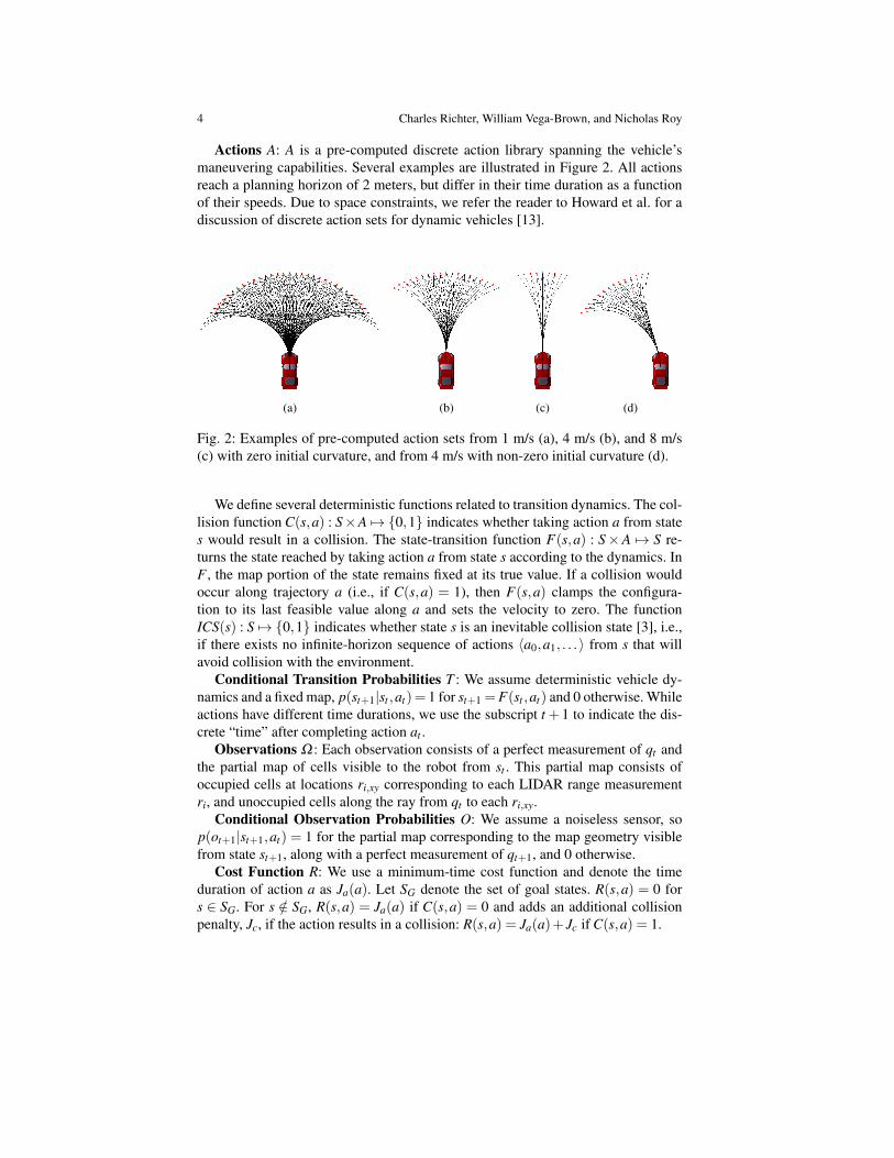
Actions A: A is a pre-computed discrete action library spanning the vehicle’smaneuvering capabilities. Several examples are illustrated in Figure 2. All actionsreach a planning horizon of 2 meters, but differ in their time duration as a functionof their speeds. Due to space constraints, we refer the reader to Howard et al. for adiscussion of discrete action sets for dynamic vehicles [13].

(a) (b) (c) (d)

Fig. 2: Examples of pre-computed action sets from 1 m/s (a), 4 m/s (b), and 8 m/s(c) with zero initial curvature, and from 4 m/s with non-zero initial curvature (d).

We define several deterministic functions related to transition dynamics. The col-lision function C(s,a) : S×A 7→ 0,1 indicates whether taking action a from states would result in a collision. The state-transition function F(s,a) : S×A 7→ S re-turns the state reached by taking action a from state s according to the dynamics. InF , the map portion of the state remains fixed at its true value. If a collision wouldoccur along trajectory a (i.e., if C(s,a) = 1), then F(s,a) clamps the configura-tion to its last feasible value along a and sets the velocity to zero. The functionICS(s) : S 7→ 0,1 indicates whether state s is an inevitable collision state [3], i.e.,if there exists no infinite-horizon sequence of actions 〈a0,a1, . . .〉 from s that willavoid collision with the environment.

Conditional Transition Probabilities T : We assume deterministic vehicle dy-namics and a fixed map, p(st+1|st ,at)= 1 for st+1 =F(st ,at) and 0 otherwise. Whileactions have different time durations, we use the subscript t +1 to indicate the dis-crete “time” after completing action at .

Observations Ω : Each observation consists of a perfect measurement of qt andthe partial map of cells visible to the robot from st . This partial map consists ofoccupied cells at locations ri,xy corresponding to each LIDAR range measurementri, and unoccupied cells along the ray from qt to each ri,xy.

Conditional Observation Probabilities O: We assume a noiseless sensor, sop(ot+1|st+1,at) = 1 for the partial map corresponding to the map geometry visiblefrom state st+1, along with a perfect measurement of qt+1, and 0 otherwise.

Cost Function R: We use a minimum-time cost function and denote the timeduration of action a as Ja(a). Let SG denote the set of goal states. R(s,a) = 0 fors ∈ SG. For s /∈ SG, R(s,a) = Ja(a) if C(s,a) = 0 and adds an additional collisionpenalty, Jc, if the action results in a collision: R(s,a) = Ja(a)+ Jc if C(s,a) = 1.

Bayesian Learning for Safe High-Speed Navigation in Unknown Environments 5

2.1 Missing prior distribution over environments

A POMDP agent maintains a belief over its state b(st) = P(qt ,m), and has a stateestimator, which computes a posterior belief that results from taking an action andthen receiving an observation, given a current belief: b(st+1) = P(st+1|bt ,at ,ot+1).If the agent’s current belief, bt , assigns uniform probability to all possible maps withindependence between map cells (a very unrealistic distribution), then an observa-tion and subsequent inference over the map distribution simply eliminates thosemaps that are not consistent with the observation and raises the uniform probabilityof the remaining possible maps. If, on the other hand, the prior belief correctly as-signs high probability to a small set of realistic maps with common structures suchas hallways, rooms, doors, etc., and low probability to the unrealistic maps, thenthis belief update may help to infer useful information about unobserved regionsof the map. For instance, it might infer that the straight parallel walls of a hallwayare likely to continue out into the unobserved regions of the map. All of this priorknowledge about the distribution of environments enters the problem through theagent’s initial belief b0, which we must somehow provide.

Unfortunately, as we noted in Section 1, modeling the distribution over real-world environments would be extremely difficult. We have little choice but to ini-tialize the robot believing that all maps are equally likely and that map cells are inde-pendent from each other. To compensate for this missing environment distribution,our approach is to learn a much more specific distribution representing the proba-bility of collision associated with a given planning scenario. This learned functionenables the agent to drive at high speed as if it had an accurate prior over environ-ments enabling reasonable inferences about the unknown. In the following sections,we will derive our learned model from the POMDP and describe how we can effi-ciently train and use this model in place of an accurate prior over environments.

2.2 Approximations to the POMDP

Let Vπ(s) = ∑∞t=0 R(st ,π(st)) be the infinite-horizon cost associated with some pol-

icy π mapping states st to actions at . The optimal cost-to-go, V ∗(s) could then, inprinciple, be computed recursively using the Bellman equation. Having computedV ∗(s) for all states, we could then recover the optimal action for a given belief1:

a∗t (bt) =argminat

∑st

b(st)R(st ,at)+

∑st

b(st) ∑st+1

P(st+1|st ,at) ∑ot+1

P(ot+1|st+1,at)V ∗(st+1)

(1)

The summations over st and ot+1 perform a state-estimation update, resulting in aposterior distribution over future states st+1 from all possible current states in ourcurrent belief bt , given our choice of action at . We can rewrite (1) as:

1 Since we use a discrete set of actions, there is a finite number of configurations that can be reachedfrom an initial configuration. Therefore, we can sum over future states rather than integrating.

6 Charles Richter, William Vega-Brown, and Nicholas Roy

a∗t (bt) = argminat

∑st

b(st)R(st ,at)+ ∑st+1

P(st+1|bt ,at)V ∗(st+1)

(2)

Since our cost function R(s,a) applies separate penalties for time and collision, wecan split V ∗(s) into two terms, V ∗(s) =V ∗T (s)+V ∗C (s), where T and C refer to “time”and “collision”. V ∗T (s), gives the optimal time-to-go from s, regardless of whethera collision occurs between s and the goal. We assume that if a collision occurs, therobot can recover and proceed to the goal. Furthermore, we assume that the optimaltrajectory from s to the goal will avoid collision if possible. But there will be somestates s for which collision is inevitable (ICS(s) = 1) since the robot’s abilities tobrake or turn are limited to finite, realistic values. Since we assume that collisionsonly occur from inevitable collision states, we can rewrite the total cost-to-go as:V ∗(s) =V ∗T (s)+ Jc · ICS(s). Substituting this expression, we can rewrite (2) as:

a∗t (bt) =argminat

∑st

b(st)R(st ,at)+

∑st+1

P(st+1|bt ,at)V ∗T (st+1)+ Jc ·∑st+1

P(st+1|bt ,at)ICS(st+1)

(3)

The first term in equation (3) is the expected immediate cost of the current action, at .We assume no collisions occur along at since the robot performs collision checkingwith respect to observed obstacles, and it nearly always perceives obstacles in theimmediate vicinity. This term simply reduces to Ja(at), the time duration of at .

The second and third terms of (3) are expected values with respect to the possiblefuture states, given at and bt . However, as we have observed in Section 2.1, ourinitial uniform belief over maps means that bt will be very unhelpful (and indeedmisleading) if we use it to take an expectation over future states, since the truedistribution over maps is surely far from uniform. The lack of meaningful priorknowledge over the distribution of environments, combined with the extremely largenumber of possible future states st+1, means that we must approximate these terms.

For the expected time-to-go, we use a simple heuristic function:

h(bt ,at)≈ ∑st+1

P(st+1|bt ,at)V ∗T (st+1), (4)

which performs a 2D grid search using Dijkstra’s algorithm (ignoring dynamics)from the end of action at to the goal, respecting the observed obstacles in bt , assum-ing unknown space is traversable and that the current speed is maintained. The use ofa lower-dimensional search to provide global guidance to a local planner is closelyrelated to graduated-density methods [12]. While other heuristics could be devised,we instead focus our efforts in this paper on modeling the collision probability.

The third term in equation (3), Jc ·∑st+1P(st+1|bt ,at)ICS(st+1), is the expected

future collision penalty given our current belief bt and action at . As we noted inSection 2.1, the fundamental problem is that our belief bt does not accurately capturewhich map structures are likely to be encountered in the unknown portions of the

Bayesian Learning for Safe High-Speed Navigation in Unknown Environments 7

environment. Correctly predicting whether a hallway will continue around a blindcorner, for instance, is impossible based on the belief alone. We instead turn tomachine learning to approximate this important quantity from training data:

fc(φ(bt ,at))≈ ∑st+1

P(st+1|bt ,at)ICS(st+1) (5)

The model, fc(φ(bt ,at)), approximates the probability that a collision will occur inthe future if we execute action at given belief bt . It is computed from some featuresφ(bt ,at) that summarize the relevant information contained in bt and at , for examplevehicle speed, distance to observed obstacles along at , etc. With the approximationsof all three terms in equation (3), we arrive at our receding-horizon control law:

a∗t (bt) = argminat

Ja(at)+h(bt ,at)+ Jc · fc(φ(bt ,at))

(6)

At each time step, we select a∗t minimizing (6) given the current belief bt . We be-gin to execute a∗t while incorporating new sensor data and re-planning. Next, wedescribe how we collect data and build a model to predict collision probabilities.

3 Predicting Future Collisions

In this section, we focus on learning to predict the probability of collision associ-ated with a given planning scenario, represented as a point in feature space, Φ . Weassume that for a given vehicle or dynamical system, there exists some true underly-ing probability of collision that is independent of the map and robot configuration,given features, φ . In other words, P(“collision”|φ ,q,m) = P(“collision”|φ). Underthis assumption, we can build a data set by training in any environments we wish,and the data will be equally valid in other environments that populate the same re-gions of feature space. If two data sets gathered from two different environmentsdo not share the same output distribution where they overlap in feature space, weassume that our features are simply not rich enough to capture the difference.

This assumption also implies that if an environment is fundamentally differentfrom our training environments with respect to collision probabilities, it will popu-late a different region of feature space. If the robot encounters an environment forwhich it has no relevant training data nearby in feature space, it should infer thatthis environment is unfamiliar and react appropriately. In these cases, we requirethat our learning algorithm somehow provide a safe prediction of collision probabil-ity rather than naıvely extrapolating the data from other environments. Our featuresmust therefore be sufficiently descriptive to predict collisions as well as differentiatebetween qualitatively different environment types.

Quantifying a planning scenario using a set of descriptive functions of belief-action pairs currently relies on the domain knowledge of the feature designer. Forthis paper, our features are four hand-coded functions: (a) minimum distance tothe nearest known obstacle along the action; (b) mean range to obstacle or frontierin the 60 cone ahead of the robot, averaged over several points along the action;

8 Charles Richter, William Vega-Brown, and Nicholas Roy

(c) length of the straight free path directly ahead of the robot, averaged over severalpoints along the action; and (d) speed at the end of the action. While these featureswork adequately, our method is extensible to arbitrary numbers of continuous- anddiscrete-valued features from a variety of different sources, including features thatoperate on a history of past measurements. We expect that additional features willenable more intelligent and subtle navigation behaviors.

3.1 Training procedure

To predict collision probabilities, we collect training data D= (φ1,y1),. . . ,(φN ,yN).Labels yi are binary indicators (“collision”, “non-collision”) associated with belief-action pairs, represented as points φi in feature space. To efficiently collect a largedata set, we use a simulator capable of generating realistic LIDAR scans and vehi-cle motions within arbitrary maps. The training procedure aims to generate scenar-ios that accurately emulate beliefs the planner may have at runtime, and accuratelyrepresent the risk of actions given those beliefs. While at runtime, the planner willuse a map built from a history of scans, we make the simplifying assumption that asingle measurement taken from configuration qt is enough to build a realistic mapof the area around qt , similar to one the planner might actually observe. With thisassumption, we can generate training data based on individual sampled robot con-figurations, rather than sampling extended state-measurement histories, which notonly results in more efficient training, but also eliminates the need for any sort ofplanner or random process to sample state histories.

We generate each data point by randomly sampling a feasible configuration, qt ,within a training map, and simulating the sensor from qt to generate a map estimate,and hence a belief bt . We then randomly select one of the actions, at , that is feasiblegiven the known obstacles in bt . Recall from equation (5) that our learned functionmodels the probability that a collision will occur somewhere after completing theimmediate chosen action at , i.e., the probability that state st+1 (with configurationqt+1) is an inevitable collision state. Therefore, to label this belief-action pair, werun a resolution-complete training planner from configuration qt+1 at the end of at .If there exists any feasible trajectory starting from qt+1 that avoids collision with thetrue hidden map (to some horizon), then ynew = 0, otherwise ynew = 1. Finally, wecompute features φnew(bt ,at) of this belief-action pair and insert (φnew,ynew) into D.

We use a horizon of three actions (6 m) for our training planner because if acollision is inevitable for our dynamics model, it will nearly always occur withinthis horizon. We have explored other settings for this horizon and found the resultsto be comparable, although if the horizon is too short, some inevitable collisionstates will be mis-labeled as “non-collision”.

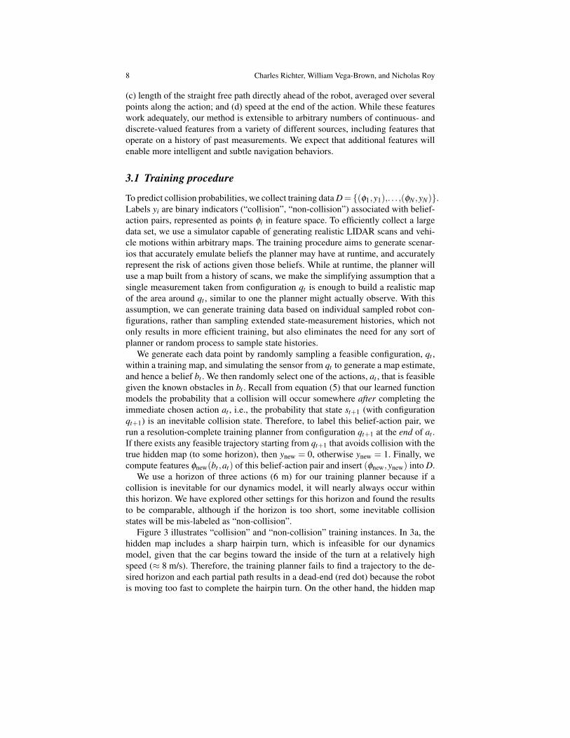
Figure 3 illustrates “collision” and “non-collision” training instances. In 3a, thehidden map includes a sharp hairpin turn, which is infeasible for our dynamicsmodel, given that the car begins toward the inside of the turn at a relatively highspeed (≈ 8 m/s). Therefore, the training planner fails to find a trajectory to the de-sired horizon and each partial path results in a dead-end (red dot) because the robotis moving too fast to complete the hairpin turn. On the other hand, the hidden map

Bayesian Learning for Safe High-Speed Navigation in Unknown Environments 9

(a) (b)

Fig. 3: Examples of “collision” (a) and “non-collision” (b) training events. One ofthe immediate actions (black) is chosen for labeling. The training planner deter-mines whether the end of this action (purple dot) is an inevitable collision state withrespect to the hidden map (shown in light gray). Feasible partial paths are shown inblue. Nodes successfully expanded by the training planner are green, and nodes forwhich no collision-free outgoing action exists are red. In (a), all partial paths dead-end (red nodes) before reaching the desired three-action horizon because the vehiclespeed is too great to complete the turn given curvature and cuvature rate limits. In(b), the training planner successfully finds a sequence of three actions.

in 3b has a straight hallway rather than a sharp turn, and the training planner suc-ceeds in finding a feasible trajectory to the three-action horizon, aided by the car’sinitial configuration toward the outside of the turn. The empirical distribution of“collision” and “non-collision” labels collected from these sampled scenarios there-fore implicitly captures the relevant environmental characteristics of the true hiddenmap distribution, and the way they interact with our dynamics model, in a muchmore efficient way than modeling the complex, high-dimensional map distributionexplicitly. Our training procedure captures sensible patterns, for instance that it issafe to drive at high speeds in wide open areas and long straight hallways, but thatslower speeds are safer when approaching a wall or navigating dense clutter.

3.2 Learning algorithm

We use a non-parametric Bayesian inference model developed by Vega-Brown etal., which generalizes local kernel estimation to the context of Bayesian inferencefor exponential family distributions [29]. The Bayesian nature of this model willenable us to provide prior knowledge to make safe (though perhaps conservative)predictions in environments where we have no training data. We model collision as aBernoulli-distributed random event with beta-distributed parameter θ ∼Beta(α,β ),where α and β are prior pseudo-counts of collision and non-collision events, re-spectively. Using the inference model from Vega-Brown et al., we can efficiently

10 Charles Richter, William Vega-Brown, and Nicholas Roy

compute the posterior probability of collision given a query point φ and data D:

fc(φ) = P(y = “collision”|φ ,D) =α(φ)+∑

Ni=1 k(φ ,φi)yi

α(φ)+β (φ)+∑Ni=1 k(φ ,φi)

, (7)

where k(φ ,φi) is a kernel function measuring proximity in feature space between ourquery, φ , and each φi in D. We use a polynomial approximation to a Gaussian ker-nel with finite support. We write prior pseudo-counts as functions α(φ) and β (φ),since they may vary across the feature space. We use the effective number of nearbytraining data points, Neff. = ∑

Ni=1 k(φ ,φi), as a measure of data density. The prior

contributes Npr. pseudo data points to each prediction, where Npr. = α(φ)+β (φ).The ratio Neff./(Neff.+Npr.) determines the relative influence of the training data andthe prior in each prediction. For data sets with 5×104 points in total, Neff. tends tobe 102 or greater when the testing environment is similar to the training map, andNeff. 1 when the testing environment is fundamentally different (i.e., office build-ing vs. natural forest). For this paper, we used Npr. = 5, and results are insensitive tothe exact value of Npr. as long as Neff. Npr. or Neff. Npr..

Machine learning algorithms should make good predictions for query points neartheir training data in input space. However, predictions that extrapolate beyond thedomain of the training data may be arbitrarily bad. For navigation tasks, we wantour planner to recognize when it has no relevant training data, and automaticallyrevert to safe behaviors rather than making reckless, uninformed predictions. Forinstance, if the agent moves from a well-known building into the outdoors, where ithas not trained, we still want the learning algorithm to guide it away from danger.

Fortunately, the inference model of equation (7) enables this capability throughthe prior functions α(φ) and β (φ). If we query a feature point in a region ofhigh data density (Neff. Npr.), fc(φ) will tend to a local weighted average ofneighbors and the prior will have little effect. However, if we query a point farfrom the training data (Neff. Npr.), the prior will dominate. By specifying pri-ors α(φ) and β (φ) that are functions of our features, we can endow the plannerwith domain knowledge and formal rules about which regions of feature space aresafe and dangerous. In this paper, we have designed our prior functions α(φ) andβ (φ) such that P(“collision”) = α(φ)/(α(φ)+ β (φ)) = 0 if there exists enoughfree space for the robot to come safely to a stop from its current velocity, andP(“collision”) =α(φ)/(α(φ)+β (φ))> 0 otherwise. Computing this prior uses theinformation in features (c) and (d) described in Section 3. Therefore, as Neff. dropsto zero (and for sufficiently large values of Jc), the learning algorithm activates aconventional stopping distance constraint, seamlessly turning our planner into onewith essentially the same characteristics as the baseline planner we compare against.

Another natural choice of learning algorithm in this domain would be a Gaus-sian process (GP). However, classification with a GP requires approximate inferencetechniques that would likely be too slow to run online, whereas the inference modelin equation (7) is an approximate model that allows efficient, analytical inference.

Bayesian Learning for Safe High-Speed Navigation in Unknown Environments 11

4 Results

We have obtained simulation results from randomly generated maps as well as ex-perimental results on a real RC car navigating as fast as 8 m/s in laboratory, officeand large open atrium environments at MIT. Our simulation and experimental re-sults both show that replacing safety constraints with a learned model of collisionprobability can result in faster navigation without sacrificing empirical safety. Theresults also show that when the planner departs a region of feature space for whichit has training data, our prior keeps the robot safe. Finally, our experiments demon-strate that even within a single real-world environment, it is easy to encounter someregions of feature space for which we have training data and others for which we donot, thereby justifying our Bayesian approach and use of prior knowledge.

4.1 Simulation Results

In this section, we present simulation results from hallway and forest environmentsthat were randomly sampled from environment-generating distributions [21]. Weuse a Markov chain to sample hallways with a width of 2.5 m and a turn frequencyof 0.4, and a Poisson process to sample 2D forests with an average obstacle rateof 0.05 trees ·m−2 and tree radius of 1 m. Figure 5 shows a randomly sampledhybrid environment composed of both hallway and forest segments. To measure thebenefit of our learned model, we compare against the baseline planner, illustratedin Figures 1a-1b, that enforces a safety constraint. This planner navigates as fast asis possible given that constraint, and represents the planner we would use if we didnot have a learned model of collision probability.

0 0.2 0.4 0.6 0.8 1

1

1.2

1.4

1.6

1.8

2

Velo

city (

Norm

aliz

ed)

Cost of Collision: Jc

0 0.2 0.4 0.6 0.8 1

0

0.2

0.4

0.6

0.8

1

Cost of Collision: Jc

Fra

ction C

rashed

0 0.2 0.4 0.6 0.8 10

2

4

6

8

Constr

ain

t V

iola

tion (

m)

Cost of Collision: Jc

Data Only

Prior Only

Data + Prior

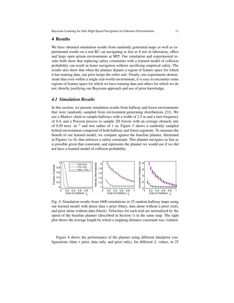
Fig. 4: Simulation results from 1600 simulations in 25 random hallway maps usingour learned model with dense data + prior (blue), data alone without a prior (red),and prior alone without data (black). Velocities for each trial are normalized by thespeed of the baseline planner (described in Section 1) in the same map. The rightplot shows the average length by which a stopping-distance constraint was violated.

Figure 4 shows the performance of the planner using different data/prior con-figurations (data + prior, data only, and prior only), for different Jc values, in 25

12 Charles Richter, William Vega-Brown, and Nicholas Roy

randomly sampled hallway environments. The training data set used for these trialswas collected in a separate hallway environment drawn from the same distribution.For low values of Jc all three planners crash in every trial, but become safer asJc is increased. Above Jc = 0.25, all planners succeed in reaching the goal with-out collision 100% of the time. At Jc = 0.25, our solution navigates approximately80% faster than baseline using data + prior, or data alone. In these trials, the priorcontributes very little since the planner has dense training data from the same envi-ronment type. The right plot illustrates average violation of a stopping-distance con-straint. For Jc = 0.25, the planners using training data violate the stopping-distanceconstraint by 5.75 m on average, indicating the degree to which this constraint isoverly conservative, given our collision probability model. The planner using theprior alone chooses not to violate the stopping distance constraint by nearly as much,and essentially converges to the baseline performance as Jc is increased.

0 100 200 300 400 500

10−1

100

101

102

103

Ne

ff. +

Np

r.Data + Prior, N

pr. = 5

0 100 200 300 400 5000

10

Velo

city (

m/s

)

Time Step

0 50 100 150 200

10−1

100

101

102

103

Data Only, Npr.

<< 1

Ne

ff. +

Np

r.

0 50 100 150 2000

10

Velo

city (

m/s

)

Time Step

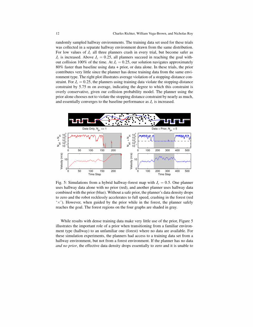
Fig. 5: Simulations from a hybrid hallway-forest map with Jc = 0.5. One planneruses hallway data alone with no prior (red), and another planner uses hallway datacombined with the prior (blue). Without a safe prior, the planner’s data density dropsto zero and the robot recklessly accelerates to full speed, crashing in the forest (red‘×’). However, when guided by the prior while in the forest, the planner safelyreaches the goal. The forest regions on the four graphs are shaded in gray.

While results with dense training data make very little use of the prior, Figure 5illustrates the important role of a prior when transitioning from a familiar environ-ment type (hallway) to an unfamiliar one (forest) where no data are available. Forthese simulation experiments, the planners had access to a training data set from ahallway environment, but not from a forest environment. If the planner has no dataand no prior, the effective data density drops essentially to zero and it is unable to

Bayesian Learning for Safe High-Speed Navigation in Unknown Environments 13

distinguish between safe and risky behaviors2. Therefore the planner accelerates tofull speed resulting in a crash (red ‘×’). However, using our Bayesian approach, theeffective number of data points drops only as low as Npr. = 5 when the agent entersthe forest and the planner is safely guided by the information in the prior. In 25 trialsof random hallway-forest maps, 100% succeeded using the prior, while only 12%succeeded without the prior.

4.2 Experimental Results

We conducted experiments on an RC car using a training dataset generated in sim-ulation on a hallway-type environment. We performed state estimation by fusing aplanar LIDAR and an IMU in an extended Kalman filter (EKF) [7]. We use theLIDAR to provide relative pose updates to the EKF using a scan-matching al-gorithm [4]. We use a Hokuyo UTM-30LX LIDAR, a Microstrain 3DM-GX3-25IMU and an Intel dual-core i7 computer with 16GB RAM. Video of our experi-mental demonstrations, at speeds up to 8.2 m/s is available at: http://groups.csail.mit.edu/rrg/bayesian_learning_high_speed_nav.

0 5 10 15 20 25

0

2

4

6

Velo

ctiy (

m/s

)

Time (s)

Baseline

Learned

Fig. 6: Experiment in which our planner (blue) reached its goal over 2x faster thanbaseline (red). Velocity profiles and trajectories for each planner are shown.

We conducted tests to show that our planner can indeed navigate faster in cer-tain real environments than the baseline planner. For the experiment shown here,we chose a narrow path within a lab space with several sharp turns and many ob-stacles. Figure 6 shows the trajectories and velocity profiles of both planners. Thebaseline planner has difficulty navigating quickly in this environment because freespace is occluded from the sensor view by obstacles. Since the baseline planner mustenforce the existence of emergency-stopping trajectories lying within the observedfree space, it is forced to move very slowly. In the velocity profile, the baseline plan-ner frequently applies the brakes to slow to about 1 m/s , whereas our planner usesits training data from the simulated hallway environment to predict that it is safe totravel up to about 3 m/s around most corners and therefore maintains a higher aver-

2 We implement the no-prior case by setting prior values of α and β each to 0.0005 to ensure thesolution is computable in regions of feature space with no data at all. The default prediction withno data is therefore P(“collision”) = α/(α +β ) = 0.5, rather than undefined if α = β = 0.

14 Charles Richter, William Vega-Brown, and Nicholas Roy

age speed. The baseline planner took 23.7 s to reach the goal in this case, whereasour planner took 11.5 s, representing a factor of two improvement.

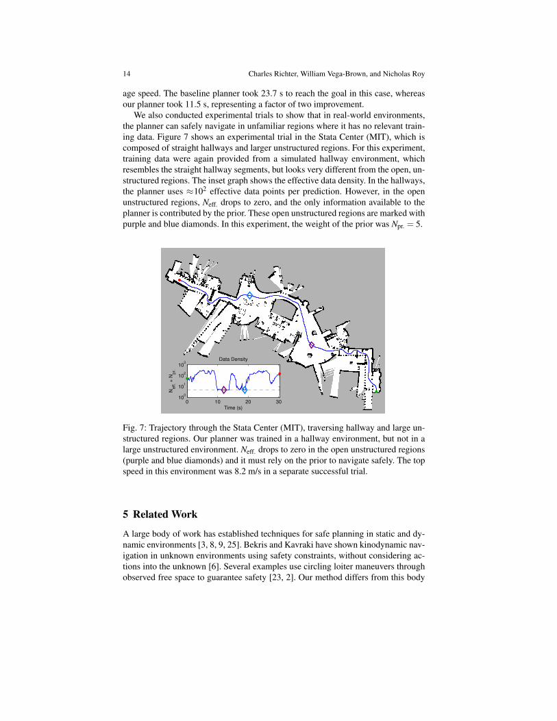
We also conducted experimental trials to show that in real-world environments,the planner can safely navigate in unfamiliar regions where it has no relevant train-ing data. Figure 7 shows an experimental trial in the Stata Center (MIT), which iscomposed of straight hallways and larger unstructured regions. For this experiment,training data were again provided from a simulated hallway environment, whichresembles the straight hallway segments, but looks very different from the open, un-structured regions. The inset graph shows the effective data density. In the hallways,the planner uses ≈102 effective data points per prediction. However, in the openunstructured regions, Neff. drops to zero, and the only information available to theplanner is contributed by the prior. These open unstructured regions are marked withpurple and blue diamonds. In this experiment, the weight of the prior was Npr. = 5.

0 10 20 3010

0

101

102

103

Data Density

Time (s)

Ne

ff. +

Np

r.

Fig. 7: Trajectory through the Stata Center (MIT), traversing hallway and large un-structured regions. Our planner was trained in a hallway environment, but not in alarge unstructured environment. Neff. drops to zero in the open unstructured regions(purple and blue diamonds) and it must rely on the prior to navigate safely. The topspeed in this environment was 8.2 m/s in a separate successful trial.

5 Related Work

A large body of work has established techniques for safe planning in static and dy-namic environments [3, 8, 9, 25]. Bekris and Kavraki have shown kinodynamic nav-igation in unknown environments using safety constraints, without considering ac-tions into the unknown [6]. Several examples use circling loiter maneuvers throughobserved free space to guarantee safety [23, 2]. Our method differs from this body

Bayesian Learning for Safe High-Speed Navigation in Unknown Environments 15

of work by relaxing absolute safety constraints and replacing them with predictionsof collision probability, which can be viewed as a form of data-driven constraints.Althoff et al. propose a collision probability concept similar to fc(φ(bt ,at)) for dy-namic environments, but they assume a known distribution over the future behaviorof each moving agent, which we do not have in the case of unknown maps [1].

In the exploration literature, the primary objective is to build a map, and actionsmay be taken to view unseen parts of the environment [30, 28]. Some explorationwork has balanced the objectives of information gain, navigation cost and localiza-tion quality from a utility or decision-theory point of view [16, 26]. Unlike explo-ration, our objective is to reach a goal in minimum time, which places emphasis oncollision probability and high-speed dynamics, rather than map information.

A natural way to reason about planning in an unknown map is through thePOMDP formalism [14]. Despite notorious complexity, various strategies havegrown the size of (approximately) solvable POMDPs [19, 15, 24]. However, wecannot simply apply POMDP techniques since we assume no explicit knowledgeof the environment distribution, or black-box simulation capabilities to sample theworld at planning time. Instead, we must learn a function of this missing distribu-tion offline. POMDPs have been used for aircraft collision avoidance [27, 5], wherea very large negative reward discourages collisions at nearly any cost. In contrast,we use small collision penalties to drive aggressively, trading off risk and reward.

Learning has been applied to autonomous vehicle navigation in several con-texts. One example from the DARPA LAGR program used deep learning to classifytraversable terrain up to 100 m away [11]. Neural networks and monocular depthestimation coupled with policy search [18, 17], as well as human-pilot demonstra-tions [22], have been used to learn high-speed reactive controllers to avoid obstacles,however these systems map sensory input directly to actions. They are not decision-theoretic planners, and do not trade off meaningfully between risk and reward.

6 Conclusion

We have shown that by using a Bayesian learning algorithm, with safety constraintsencoded as a prior over collision probabilities, our planner can detect when it lacksthe appropriate training data for its environment and seamlessly revert to safe be-haviors. Our strategy offers a simple and elegant probabilistic method of mergingthe performance benefits of training experience with the the reassurance of safetyconstraints when faced with an unfamiliar environment. One of the main limitationsof this work is the difficulty of hand-coding feature functions that describe complexplanning scenarios. We plan to address this limitation by applying recent feature-learning techniques to automatically generate feature functions from data, extendingour methods to handle different scenarios, map representations and sensor types.

References

1. D. Althoff et al. Safety assessment of robot trajectories for navigation in uncertain and dy-namic environments. Autonomous Robots, 32(3):285-302, 2012.

16 Charles Richter, William Vega-Brown, and Nicholas Roy

2. S. Arora et al. A principled approach to enable safe and high performance maneuvers forautonomous rotorcraft. American Helicopter Society 70th Annual Forum, 2014.

3. H. Asama and T. Fraichard. Inevitable collision states - a step towards safer robots. AdvancedRobotics, 18:1001–1024, 2004.

4. A. Bachrach et al. RANGE - robust autonomous navigation in GPS-denied environments.Journal of Field Robotics, 28(5):644–666, 2011.

5. H. Bai et al. Unmanned aircraft collision avoidance using continuous-state POMDPs. In Proc.Robotics: Science & Systems, 2011.

6. K. E. Bekris and L. E. Kavraki. Greedy but safe replanning under kinodynamic constraints.In Proc. ICRA, 2007.

7. A. Bry et al. State estimation for aggressive flight in GPS-denied environments using onboardsensing. In Proc. ICRA, 2012.

8. P. Fiorini and Z. Shiller. Motion planning in dynamic environments using velocity obstacles.International Journal of Robotics Research, 17(7):760–772, 1998.

9. D. Fox et al. The dynamic window approach to collision avoidance. IEEE Robotics & Au-tomation Magazine, 4(1):23–33, 1997.

10. T. Fraichard. A short paper about motion safety. In Proc. ICRA, 2007.11. R. Hadsell, et al. Learning long-range vision for autonomous off-road driving. Journal of

Field Robotics, 26(2):120–144, 2009.12. T. M. Howard et al. Model-Predictive Motion Planning: Several Key Developments for Au-

tonomous Mobile Robots. Robotics Automation Magazine, IEEE, 21(1):64–73, 2014.13. T. M. Howard et al. State space sampling of feasible motions for high-performance mobile

robot navigation in complex environments. Journal of Field Robotics, 25(6-7):325–345, 2008.14. L. P. Kaelbling et al. Planning and acting in partially observable stochastic domains. Artificial

intelligence, 101(1):99–134, 1998.15. H. Kurniawati et al. SARSOP: Efficient point-based POMDP planning by approximating

optimally reachable belief spaces. In Proc. Robotics: Science & Systems, 2008.16. A. A. Makarenko et al. An experiment in integrated exploration. In Proc. IROS, 2002.17. J. Michels et al. High speed obstacle avoidance using monocular vision and reinforcement

learning. In Proc. ICML, 2005.18. U. Muller et al. Off-road obstacle avoidance through end-to-end learning. In Proc. NIPS,

2005.19. J. Pineau et al. Point-based value iteration: An anytime algorithm for POMDPs. In Proc.

IJCAI, 2003.20. C. Richter et al. High-speed autonomous navigation of unknown environments using learned

probabilities of collision. In Proc. ICRA, 2014.21. C. Richter et al. Markov chain hallway and Poisson forest environment generating distribu-

tions. Technical Report MIT-CSAIL-TR-2015-014, 2015.22. S. Ross et al. Learning monocular reactive UAV control in cluttered natural environments. In

Proc. ICRA, 2013.23. T. Schouwenaars et al. Receding horizon path planning with implicit safety guarantees. In

Proc. ACC, 2004.24. D. Silver and J. Veness. Monte-carlo planning in large POMDPs. In Proc. NIPS, 2010.25. R. Simmons. The curvature-velocity method for local obstacle avoidance. In Proc. ICRA,

1996.26. C. Stachniss et al. Information gain-based exploration using Rao-Blackwellized particle fil-

ters. In Proc. Robotics: Science & Systems, 2005.27. S. Temizer et al. Collision avoidance for unmanned aircraft using Markov decision processes.

In AIAA Guidance, Navigation, and Control Conference, 2010.28. S. Thrun et al. Map learning and high-speed navigation in RHINO. AI-based Mobile Robots:

Case studies of successful robot systems. MIT Press, Cambridge, MA, 1998.29. W. Vega-Brown et al. Nonparametric Bayesian inference on multivariate exponential families.

In Proc. NIPS, 2014.30. B. Yamauchi. A frontier-based approach for autonomous exploration. In Proc. Computational

Intelligence in Robotics and Automation, 1997.