Bayesian Instruments Via Dirichlet Process Priors Peter Rossi GSB/U of Chicago joint with Rob...

Bayesian Instruments Via Dirichlet Process Priors

Peter RossiGSB/U of Chicago

joint with Rob McCulloch, Tim Conley, and Chris Hansen

2

MotivationIV problems are often done with a “small” amount of sample information (weak ins).

It would seem natural to apply a small amount of prior information, e.g. the returns to education are unlikely to be outside of (.01, .2).

Another nice example– instruments are not exactly valid. They have some small direct correlation with the outcome/unobservables.

BUT, Bayesian methods (until now) are tightly parametric. Do I always have to make the efficiency/consistency tradeoff?

3

OverviewConsider parametric (normal) model first

Consider finite mixture of normals for error dist

Make the number of mixture components random and possibly “large”

Conduct sampling experiments and compare to state of the art classical methods of inference

Consider some empirical examples where being a non-parametric Bayesian helps!

4

The Linear Case

1

2

1

2

x z

y x

2 2 2cov , 0 ~x x

Linear Structural equations are central in applied work.

99-04, QJE/AER/JPE had 129 articles with Linear model, 89 with only one endog RHS var! This is a relevant and simple ex:

1

2

~ 0,N

(1)is a regression equation.

(2)is not !!

1 1~z

5

The Likelihood

1

1 2

1

2'

x z

y z

Derive the joint distribution of y, x | z.

or

, , , , ,p x y

1

2

1

2'x

y

x z v

y z v

1

2

~ 0,

1 0';

1

vN

v

A A A y

x

6

Identification Problems – “Weak” instruments

Suppose . 0

1

1 2

x

y

11 12

12

11 11

cov ,

cov ,

x y

or

x y

small, trouble!

7

Priors

Which parameterization should you use?

Are independent priors acceptable?

, ,

, ,x y x y

p p p p

p p p preference prior situation

8

A Gibbs Sampler

Tricks (rivGibbs in bayesm):

(1)given , convert structural equation into standard Bayes regression. We “observe” Compute .

(2)given β, we have a two regressions with same coefficients or a restricted MRM.

1 , , , ,

2 , , , ,

3 , , , ,

x y z

x y z

x y z

12 1

9

Gibbs Sampler: beta draw

Given , we observe . We rewrite the structural equation as

, , , ,x y z

1

2 1

2 1y x

where refers to the conditional distribution of given .

2

2 2

2212 12

2 1 1 2 2211 11

121 2

11

; v

v v

v

y x v

12

10

Gibbs Sampler: delta draw , , , ,x y z

1

1 2 1 2

1

1 2

2

; ' '

;

x z

y z or y z

v Var v A A LL

v Lu Var u I

Standardize the two equations and we have a restricted MRM (estimate by “doubling” the rows):

1 1

x zL L u

y z

11

Weak Ins Ex

VERY weak (Rsq=0.01)

(rel num eff = 10)

Influence of very diffuse but proper prior on -- shrinks corrs to 0.

0.5 1.0 1.5 2.0

-0.5

0.0

0.5

1.0

beta

s12o

s11

-0.5 0.0 0.5 1.0

-0.5

0.0

0.5

1.0

s12os11

delta

0.5 1.0 1.5 2.0

-0.5

0.0

0.5

1.0

beta

delta

0 200 400 600 800 10000.

51.

01.

52.

0

beta

12

Weak Ins Ex

Posteriors based on 100,000 draws

Inadequacy of Standard Normal Asymptotic Approximations!

beta

-6 -4 -2 0 2 4 6

020

0040

0060

00

delta

-0.5 0.0 0.5 1.0

050

0010

000

1500

0

s12os11

-4 -2 0 2 4 6 8

020

0040

0060

00

13

Using Mixtures of Normals

We can implement exact sample Bayesian inference with normal errors

However, our friends in econometrics tell us –

don’t like making distribution assumptions.

willing to accept loss of efficiency.

willing to ignore adequacy of asymptotics issue or search for different asymptotic experiments (e.g. weak ins asymptotics).

Can we be “non-parametric” without loss of efficiency?

14

Mixtures of Normal for Errors

'1

'2

'1'2

~ ,

~ ( )

ind ind

x z

y x

N

ind multinomial p

Consider the instrumental variables model with mixture of normal errors with K components:

' '

1note: E and E

K

ind k kkind E ind p

15

Identification with Normal Mixtures The normal mixture model for the errors is not identified. A standard unconstrained Gibbs Sampler will exhibit “label-switching.”

One View: Not an issue, error density is a nuisance parameter. Coefs of structural and instrument equations are identified.

Another View: Any function of the error density is identified. GS will provide the posterior distribution of the density ordinates.

Constrained samplers will often exhibit inferior mixing properties and are unnecessary here.

16

A Gibbs Sampler

Tricks:

Need to deal with fact that errors have non-zero mean

Cluster observations according to ind draw and standardize using appropriate comp parameters.

,

,

,

1 , , , , ,

2 , , , , ,

3 , , , , ,

k k

k k

k k

ind x y z

ind x y z

ind x y z

17

Gibbs Sampler: beta draw

Very similar to one comp case, except the error terms have non-zero mean and keep track of which comp each obs comes from!

, , , , ,k kind x y z

2

2 2

212,' ' ' ' 2

2, 1, 2, 1, 2, , 22,11,

12,' ' '2, 1, 2, 1, 1,

11,

' '2, 1, , ,

;

estimate:

i

i i

i

i

i i

i

i i

indi i i i i v ind ind

ind

indi i ind i ind

ind

i i i v ind i v ind i

E v

E

y E x u

18

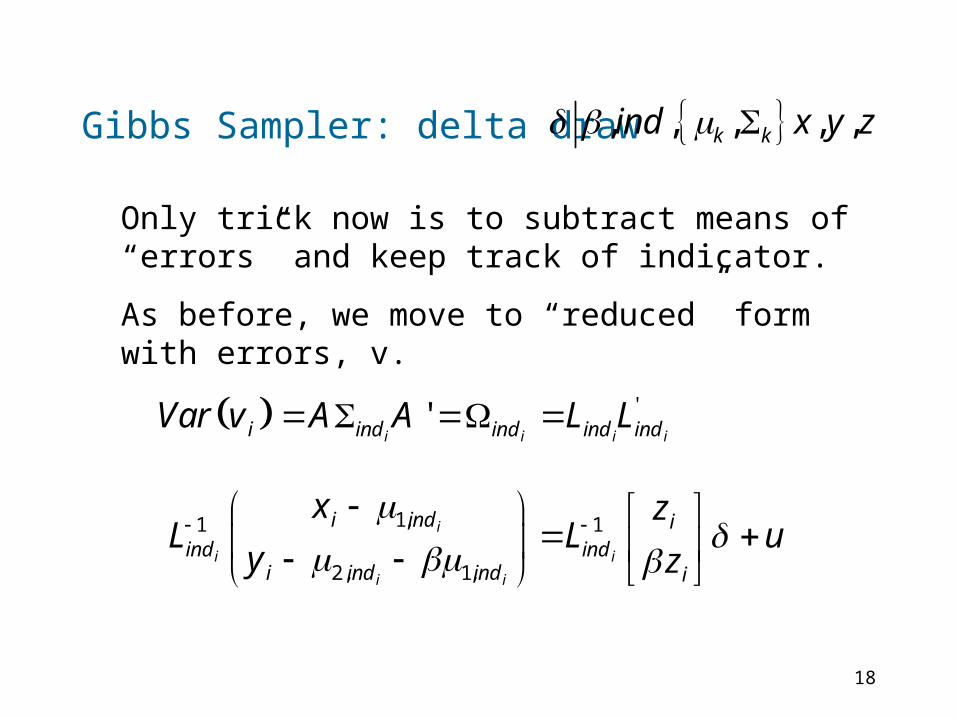
Gibbs Sampler: delta draw , , , , ,k kind x y z

Only trick now is to subtract means of “errors” and keep track of indicator.

As before, we move to “reduced” form with errors, v.

''i i i ii ind ind ind indVar v A A L L

1,1 1

2, 1,

i

i i

i i

i ind iind ind

i ind ind i

x zL L u

y z

19

Fat-tailed Example

1 1

2 2 1

' .95, .05

1 .8comp 1: '~ 0,

.8 1

comp 2: '~ 0,

p

N

N M

M Var z

Standard outlier model:

What if you specify thin tails (one comp)?

20

Fat Tails

One Comp

beta

0.0 0.2 0.4 0.6 0.8

010

020

030

0

Two Comp

beta

0.0 0.2 0.4 0.6 0.8

050

100

200

Five Comp

beta

0.0 0.2 0.4 0.6 0.8

050

150

2 1200

21

Number of Components

If I only use 2 components, I am cheating! In the plots shown earlier I used 5 components.

One practical approach, specify a relative large number of components, use proper priors.

What happens in these examples?

Can we make number of components dependent on data?

22

Dirichlet Process Model: Two Interpretations

1). DP model is very much the same as a mixture of normals except we allow new components to be “born” and old components to “die” in our exploration of the posterior.

2). DP model is a generalization of a hierarchical model with a shrinkage prior that creates dependence or “clumping” of observations into groups, each with their own base distribution.

Ref: Practical Nonparametric and Semiparametric Bayesian Statistics (articles by West and Escobar/MacEachern)

23

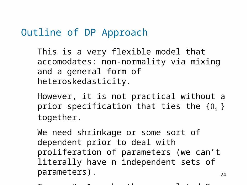
Outline of DP Approach

How can we make the error distribution flexible?

Start from the normal base, but allow each error to have it’s own set of parms:

,

1

i

n

1

i

n

1 1 1,

,i i i

,n n n

24


This is a very flexible model that accomodates: non-normality via mixing and a general form of heteroskedasticity.

However, it is not practical without a prior specification that ties the {i } together.

We need shrinkage or some sort of dependent prior to deal with proliferation of parameters (we can’t literally have n independent sets of parameters).

Two ways: 1. make them correlated 2. “clump” them together by restricting to I* unique values.

25


Consider generic hierarchical situation:

0

, ,

~i i

i G

(errors) are conditionally independent, e.g. normal with

One component normal model:

,i i i

,i

DAG:

i i

Note: thetas are indep (conditional on lambda)

,

26

G is a Dirichlet Process – a distribution over other distributions. Each draw of G is a Dirichlet Distribution. G is centered on with tightness parameter α

DP prior

Add another layer to hierarchy – DP prior for theta

0G

DAG:

i i

,

G

27

DPM

Collapse the DAG by integrating out G

1, , n

DAG:

i i

are now dependent with a mixture of DP distribution. Note: this distribution is not discrete unlike the DP. Puts positive probability on continuous distributions.

28

DPM: Drawing from Posterior

Basis for a Gibbs Sampler:

Why? Conditional Independence!

This is a simple update:

There are “n” models for each of the other values of theta and the base prior. This is very much like mixture of normals draw of indicators.

, ,j j j j j

j

29


n models and prior probs:

0

11

1

i with prior probn

G with priorprobn

0 0,, , , ~ j j

j j j

i i

q G

q i j

“birth”

one of others

30


Note: q need to be normalized! Conjugate priors can help to compute q0.

0 0 0

0 1

11

j j j j j

j j j j

i i j j i

q p M p p d p M

p G dn

q p M pn

31

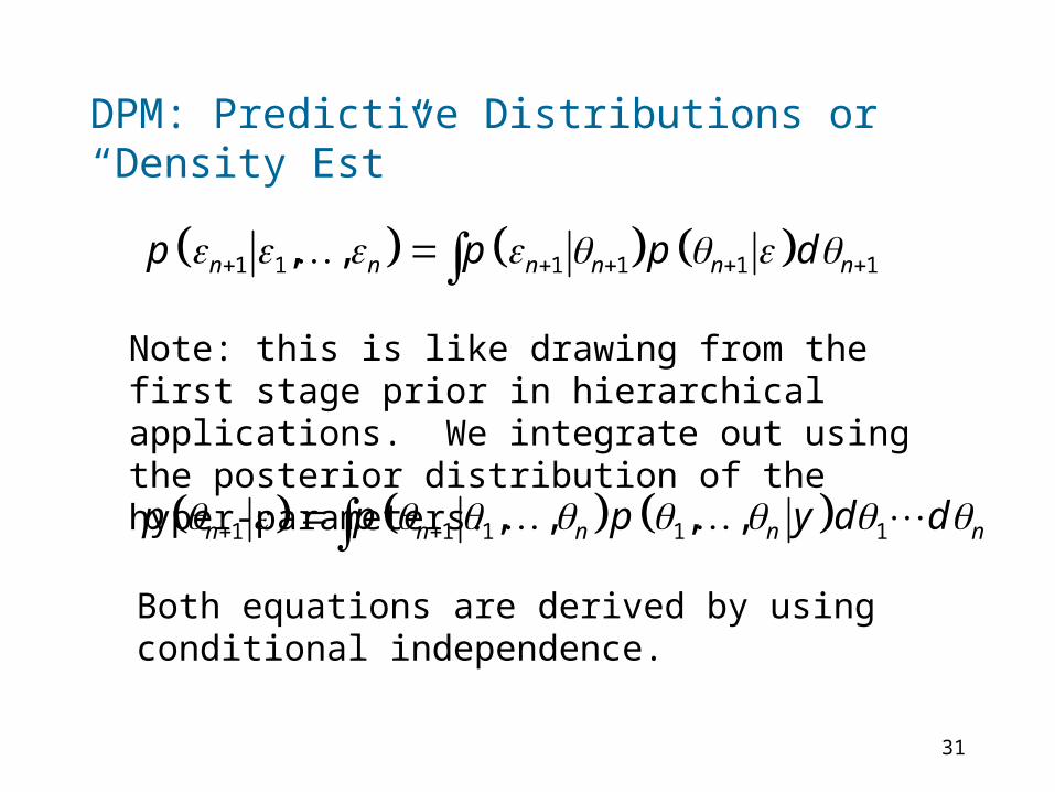
DPM: Predictive Distributions or “Density Est”

Note: this is like drawing from the first stage prior in hierarchical applications. We integrate out using the posterior distribution of the hyper-parameters.

1 1 1 1 1 1, ,n n n n n np p p d

1 1 1 1 1, , , ,n n n n np p p y d d

Both equations are derived by using conditional independence.

32

DPM: Predictive Distributions or “Density Est”

0

1

,~

1, 1, ,

n

i

with prob draw fromGn

with prob draw from i nn

Algorithm to construct predictive density:

1. draw

2. construct

3. average to obtain predictive density

1 ,rn

1 1r

n np

33

Assessing the DP prior

Two Aspects of Prior:

-- influences the number of unique values of

G0, -- govern distribution of proposed values of

e.g.

I can approximate a distribution with a large number of “small” normal components or a smaller number of “big” components.

34

Assessing the DP prior: choice of α

* ( )Pr k k

nI k Sn

There is a relationship between α and the number of distinct theta values (viz number of normal components). Antoniak (74) gives this from MDP.

S are “Stirling numbers of First Kind.” Note: S cannot be computed using standard recurrence relationship for n > 150 without overflow!

1( ) ln

kkn

nS n

k

35

Assessing the DP prior: choice of α

0 10 20 30 40 50

0.0

0.2

0.4

0.6

0.8

1.0

alpha= 0.001

Num Unique

0 10 20 30 40 50

0.00

0.05

0.10

0.15

0.20

alpha= 0.5

Num Unique

0 10 20 30 40 50

0.00

0.05

0.10

0.15

alpha= 1

Num Unique

0 10 20 30 40 50

0.00

0.02

0.04

0.06

alpha= 5

Num Unique

For N=500

36

Assessing the DP prior: Priors on α

Fixing may not be reasonable. Prior on number of unique theta may be too tight.

“Solution:” put a prior on alpha.

Assess prior by examining the priori distribution of number of unique theta.

* *p I p I p d

1p

37

Assessing the DP prior: Priors on α

0.0 0.5 1.0 1.5 2.0 2.5

0.0

00.0

20.0

40.0

60.0

8Prior on alpha

alpha

0 10 20 30 40 50

0.0

00.0

20.0

40.0

60.0

8

Implied Prior on Istar

Istar

38

Assessing the DP prior: Choice of

0 0 0 1j j j j jq p M p G dn

Both α and determine the probability of a “birth.”

Intuition:

1. Very diffuse settings of reduce model prob.

2. Tight priors centered away from y will also reduce model prob.

Must choose reasonable values. Shouldn’t be very sensitive to this choice.

39


10 : ~ , ; ~ ,G N a IW V

Choice of made easier if we center and sacle scale both y and x by the std deviation. Then we know much of mass distribution should lie in [-2,2] x [-2,2].

Set

We need assess , v, a with the goal of spreading components across the support of the errors.

2 and 0V vI

40


Look at marginals of and 1

1

Choose , ,

Pr .25 3.25 .8

Pr 10 10 .8

2.004, .17, .016

v a

v a

Very Diffuse!

41

Draws from G0

42

Gibbs Sampler for DP in the IV Model

*

*

, , , ,

, , , ,

, , , ,

, , , , ,

i

i

i

i

x y z

x y z

x y z

ind x y z

I

“Remix” Step

Same as for Normal Mixture Model

Trivial (discrete)

Doesn’t Vectorize

q computations and conjugate draws are can be vectorized (if computed in advance for unique set of thetas).

43

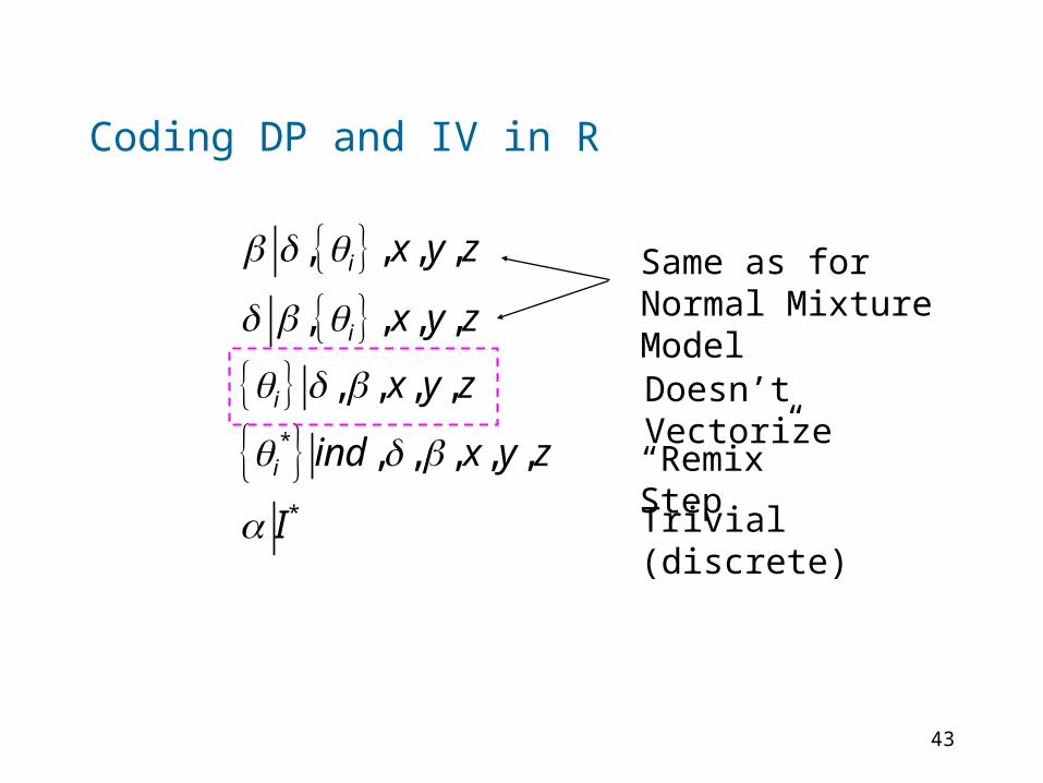
Coding DP and IV in R

*

*

, , , ,

, , , ,

, , , ,

, , , , ,

i

i

i

i

x y z

x y z

x y z

ind x y z

I

“Remix” Step

Same as for Normal Mixture Model

Trivial (discrete)

Doesn’t Vectorize

44

Coding DP and IV in R , , , ,i x y z

To draw indicators and new set of theta, we have to “Gibbs thru” each observation. We need routines to draw from the Base Prior and Posterior from “one obs” and base Prior (birth step).

We summarize each draw of using a list structure for the set of unique thetas and an indicator vector (length n).

We code the thetadraw in C but use R functions to draw from Base Posterior and evaluate densities at new theta value.

45

Coding DP and IV in R: inside rivDP

for(rep in 1:R) {

# draw beta and gamma

out=get_ytxt(y=y,z=z,delta=delta,x=x,

ncomp=ncomp,indic=indic,comps=comps)

beta = breg(out$yt,out$xt,mbg,Abg)

# draw delta

out=get_ytxtd(y=y,z=z,beta=beta,

x=x,ncomp=ncomp,indic=indic,comps=comps,dimd=dimd)

delta = breg(out$yt,out$xtd,md,Ad)

# DP process stuff- theta | lambda

Err = cbind(x-z%*%delta,y-beta*x)}

DPout=rthetaDP(maxuniq=maxuniq,alpha=alpha,lambda=lambda,

Prioralpha=Prior$Prioralpha,theta=theta,y=Err,

yden=reqfun$yden,q0=reqfun$q0,thetaD=reqfun$thetaD,GD=reqfun$GD)

indic=DPout$indic

theta=DPout$theta

comps=DPout$thetaStar

alpha=DPout$alpha

Istar=DPout$Istar

ncomp=length(comps)

}

46

Coding DP and IV in R: Inside rthetaDP

# initialize indicators and list of unique thetas

thetaStar=unique(theta);nunique=length(thetaStar)

q0v = q0(y,lambda,eta)

ydenmat[1:nunique,]=yden(thetaStar,y,eta)

# ydenmat is a length(thetaStar) x n array f(y[j,] | thetaStar[[i]]

# use .Call to draw theta list

theta= .Call("thetadraw",y,ydenmat,indic,q0v,p,theta,thetaStar,lambda,eta,

thetaD=thetaD,yden=yden,maxuniq,new.env())

thetaStar=unique(theta)

nunique=length(thetaStar)

newthetaStar=vector("list",nunique)

#thetaNp1 and remix

probs=double(nunique+1)

for(j in 1:nunique) {

ind = which(sapply(theta,identical,thetaStar[[j]]))

probs[j]=length(ind)/(alpha+n)

new_utheta=thetaD(y[ind,,drop=FALSE],lambda,eta)

for(i in seq(along=ind)) {theta[[ind[i]]]=new_utheta}

newthetaStar[[j]]=new_utheta

indic[ind]=j

}

# draw alpha

47

Coding DP and IV in R: Inside thetadraw.C/* start loop over observations */

for(i=0;i < n; i++){

probs[n-1]=NUMERIC_POINTER(q0v)[i]*NUMERIC_POINTER(p)[n-1];

for(j=0;j < (n-1); j++){

ii=indic[indmi[j]]; jj=i; /* find element ydenmat(ii,jj+1) */

index=jj*maxuniq+(ii-1);

probs[j]=NUMERIC_POINTER(p)[j]*NUMERIC_POINTER(ydenmat)[index];

}

ind=rmultin(probs,n);

if(ind == n){

yrow=getrow(y,i,n,ncol);

SETCADR(R_fc_thetaD,yrow);

onetheta=eval(R_fc_thetaD,rho);

SET_ELEMENT(theta,i,onetheta);

SET_ELEMENT(thetaStar,nunique,onetheta);

SET_ELEMENT(lofone,0,onetheta);

SETCADR(R_fc_yden,lofone);

newrow=eval(R_fc_yden,rho);

for(j=0;j<n; j++)

{NUMERIC_POINTER(ydenmat)[j*

maxuniq+nunique]=NUMERIC_POINTER(newrow)[j];}

indic[i]=nunique+1;

nunique=nunique+1;}

else {

onetheta=VECTOR_ELT(theta,indmi[ind-1]);

SET_ELEMENT(theta,i,onetheta);

indic[i]=indic[indmi[ind-1]];

}

}

48

Sampling Experiments

Examples are suggestive, but many questions remain:

1. How well do DP models accommodate departures to normality?

2. How useful are the DP Bayes results for those interested in “standard” inferences such as confidence intervals?

3. How do conditions of many instruments or weak instruments affect performance?

49

Sampling Experiments – Choice of Non-normal Alternatives

Let’s start with skewed distributions. Use a translated log-normal. Scale by inter-quartile range.

0 5 10 15

-20

24

68

1012

e1

e2

e1

-2 0 2 4 6 8 10

0.0

0.1

0.2

0.3

0.4

0.5

50

Sampling Experiments – Strength of Instruments- F stats

0.5 1 1.5

010

2030

40Normal Errors

delta

0.5 1 1.50

1020

30

Log-normal Errors

delta

0.5 1 1.5

0.2

0.4

0.6

0.8

Normal Errors

delta

0.5 1 1.5

0.2

0.4

0.6

0.8

Log-normal Errors

delta

Weak case is bounded away from zero. We don’t have huge numbers of data sets with no information!

weak

strong

Moderate

k=10

51

Sampling Experiments – Strength of Instruments- 1st Stage R-squared 0.5 1 1.5

010

2030

40

Normal Errors

delta

0.5 1 1.5

010

2030

Log-normal Errors

delta

0.5 1 1.5

0.2

0.4

0.6

0.8

Normal Errors

delta

0.5 1 1.5

0.2

0.4

0.6

0.8

Log-normal Errors

delta

52

Sampling Experiments- Alternative Procedures

Classical Econometrician: “We are interested in inference. We are not interested in a better point estimator.”

Standard asymptotics for various K-class estimators

“Many” instruments asymptotics (bound F as k, N increase)

“Weak” instrument asymptotics (bound F and fix k as N increases) Kleibergen (K), Modified Kleibergen (J), and Conditional Likelihood Ratio(CLR) (Andrews et al 06).

53

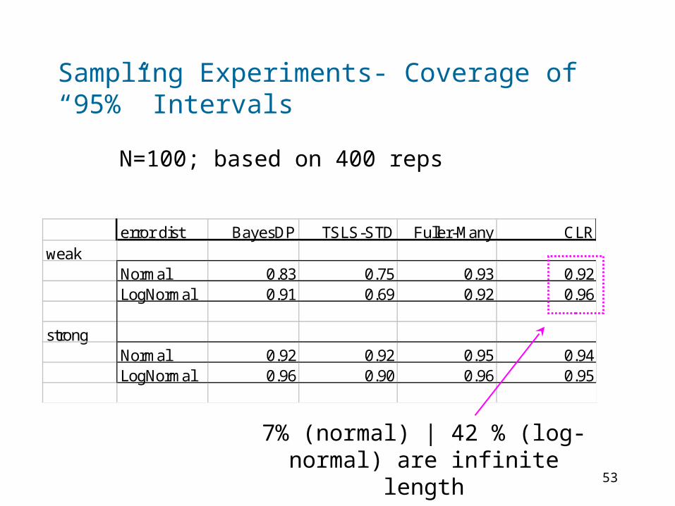
Sampling Experiments- Coverage of “95%” Intervals

error dist BayesDP TSLS-STD Fuller-Many CLRweak

Normal 0.83 0.75 0.93 0.92LogNormal 0.91 0.69 0.92 0.96

strongNormal 0.92 0.92 0.95 0.94LogNormal 0.96 0.90 0.96 0.95

7% (normal) | 42 % (log-normal) are infinite length

N=100; based on 400 reps

54

Bayes Vs. CLR (Andrews 06)

-4 -2 0 2 4

010

2030

4050

interval

sim

#

Weak Instrument

s Log-Normal Errors

55

Bayes Vs. Fuller-Many

Weak Instrument

s Log-Normal Errors

-4 -2 0 2 4

010

2030

4050

interval

sim

#

56

Infinite Intervals vs. First Stage F-test

Weak Instruments | Log-Normal Errors Case

Significant

Insignificant

Finite190 42

Infinite10 158

57

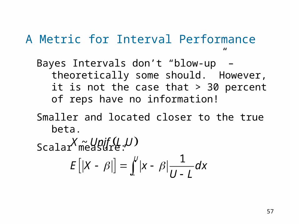
A Metric for Interval Performance

Bayes Intervals don’t “blow-up” – theoretically some should. However, it is not the case that > 30 percent of reps have no information!

Smaller and located closer to the true beta.

Scalar measure:

~ ,

1U

L

X Unif L U

E X x dxU L

58

Interval Performance

error dist BayesDP TSLS-STD Fuller-Many CLR-Weakweak



59

Estimation Performance - RMSE

Error DistBayesNP BayesDP TSLS F1

weakNormal 0.24 0.24 0.26 0.29LogNormal 0.35 0.16 0.37 0.43


Estimator

60

Estimation Performance - Bias

BayesNP BayesDP TSLS F1weak



61

An Example: Card Data

y is log wage.

x education (yrs)

z is proximity to 2 and 4 year colleges

N=3010.

Evidence from standard models is a negative correlation between errors (contrary to the old ability omitted variable interpretation).

62

An Example: Card Data Norm Errors

posterior mean = 0.185beta

0.0 0.1 0.2 0.3 0.4 0.5

050

010

0015

0020

0025

00

[ ]

DP Errors

posterior mean = 0.105beta

0.0 0.1 0.2 0.3 0.4 0.5

050

010

0015

0020

00

[ ]

63


-2 -1 0 1 2

-2-1

01

2

e1

e2

Error Density

Non-normal and low dependence.

Implies “normal” error model results may be driven by small fraction of data.

64


One-component model is “fooled” into believing there is a lot “endogeneity”

-2 -1 0 1 2

-2-1

01

2

e1

e2

One Component Normal

65

Conclusions

BayesDP IV works well under the rules of the classical instruments literature game.

BayesDP strictly dominates BayesNP

Do you want much shorter intervals (more efficient use of sample information) at the expense of somewhat lower coverage in very weak instrument case?

General approach extends trivially to allow for nonlinear structural and reduced form equations via the same device of allowing clustering of parameter values.

Bayesian Instruments Via Dirichlet Process Priors Peter Rossi GSB/U of Chicago joint with Rob...

Documents

Transcript of Bayesian Instruments Via Dirichlet Process Priors Peter Rossi GSB/U of Chicago joint with Rob...