BAYESIAN INFERENCE IN DECOMPOSABLE GRAPHICAL MODELS …1141468/FULLTEXT01.pdf · MODELS USING...

BAYESIAN INFERENCE IN DECOMPOSABLE GRAPHICAL

MODELS USING SEQUENTIAL MONTE CARLO METHODS

JIMMY OLSSON, TATJANA PAVLENKO AND FELIX L. RIOS

Abstract. In this study we present a sequential sampling methodology for Bayesianinference in decomposable graphical models. We recast the problem of graph esti-mation, which in general lacks natural sequential interpretation, into a sequentialsetting. Specifically, we propose a recursive Feynman-Kac model which generatesa flow of junction tree distributions over a space of increasing dimensions anddevelop an efficient sequential Monte Carlo sampler. As a key ingredient of theproposal kernel in our sampler we use the Christmas tree algorithm developed inthe companion paper Olsson et al. [2017]. We focus on particle MCMC methods,in particular particle Gibbs (PG) as it allows for generating MCMC chains withglobal moves on an underlying space of decomposable graphs. To further improvethe algorithm mixing properties of this PG, we incorporate a systematic refresh-ment step implemented through direct sampling from a backward kernel. Thetheoretical properties of the algorithm are investigated, showing in particular thatthe refreshment step improves the algorithm performance in terms of asymptoticvariance of the estimated distribution. Performance accuracy of the graph esti-mators are illustrated through a collection of numerical examples demonstratingthe feasibility of the suggested approach in both discrete and continuous graphicalmodels.

1. Introduction

Graphical models provide a convenient framework for representing conditional in-dependencies of a multivariate distribution which allows for efficient computationalmethods of for example conditional and marginal distributions. In this paper we focuson inferring the graph distribution purely from the data in a Bayesian perspective,a process referred to as Bayesian graph structure learning. We consider the classof decomposable graphical models which have benefited from a great deal of interestdue to their distributional properties. Specifically the factorisation of the distributionover cliques and separators make these models especially attractive for approximateBayesian inference, see e.g. Dawid and Lauritzen [1993], Rajaratnam et al. [2008].

The common strategy to approximate the graph posterior comprises the class ofMCMC methods such as the Metropolis-Hastings sampling scheme. These methods,by local moves on the edge set, generate MCMC chains by either operating directly onthe space of decomposable graph or their corresponding junction trees, see for exampleGreen and Thomas [2013], Giudici and Green [1999], Dellaportas and Forster [1999].

1

2 JIMMY OLSSON, TATJANA PAVLENKO AND FELIX L. RIOS

However, these samplers as well as other MCMC strategies based on local movesoften suffer from bad mobility. To tackle this issue, we recast the problem of graphestimation, which in general lacks natural sequential interpretation, into a sequentialsetting by an auxiliary construction which we will refer to as temporalisation relyingpartly on the methodology of SMC samplers Del Moral et al. [2006]. Specifically,we suggest a recursive Feynman-Kac model which generates a flow of junction treedistributions over a space of increasing dimensions and develop an efficient sequentialMonte Carlo (SMC) sampler. The corner stone in the proposal kernel of the SMCalgorithm is the Christmas tree algorithm (CTA) presented in the companion paperOlsson et al. [2017]. The CTA, is based on a Markovian transition kernel definedon the space of junction tress which dominates the Feynman-Kac transition kernelconstructed by the temporalisation. The motivation of operating over the space ofjunction trees is the tractability of the proposal probability that is guaranteed by theCTA; this property seems to be hard to obtain by operating directly on the space ofdecomposable graphs.

Our SMC algorithm is then incorporated as an inner loop in a particle Gibbs (PG)sampler. In order to reduce the variance of and improve the mobility of the standardPG sampler, we further introduce a step of systematic refreshment step in terms ofbackwards sampling.

The rest of the paper is structured as follows. In Section 2 we introduce somenotation and present some standard theoretical results for decomposable graphs andtheir junction tree representations. In Section 3 we specify the family of distributionsover decomposable graphical models suitable for Bayesian structural inference andpresent a number of motivating examples. Section 4 presents a four stage strategyfor the temporalisation of decomposable models. The SMC sampler is designed inSection 5 along with the standard PG and its systematic refreshment extension. InSection 6 we investigate numerically the performance of the suggested PG samplerfor three examples of Bayesian structure learning in decomposable graphical models.

2. Preliminaries

2.1. Some notation. We will always assume that all random variables are well de-fined on a common probability space (Ω,F ,P). We denote by N∗ the positive nat-ural numbers, and for any (m,n) ∈ N2 we use Jm,nK to denote the unordered setm, . . . , n. By R∗+ we denote the positive real numbers.

Measurable spaces. Given some measurable space (X,X ), we denote by M(X ) andM1(X ) the sets of measures and probability measures on (X,X ), respectively. In thecase where X is a finite set, X is always assumed to be the power set ℘(X) of X, andwe simply write M(X) and M1(X) instead of M(℘(X)) and M1(℘(X)), respectively.In the finite case, counting measures will be denoted by |dx|. We let F(X ) the set ofmeasurable functions on (X,X ).

BAYESIAN INFERENCE IN DECOMPOSABLE MODELS USING SMC METHODS 3

Kernel notation. Let µ be a measure on some measurable space (X,X ). Then for anyµ-integrable function h, we use the standard notation

µh :=

∫h(x)µ(dx)

to denote the Lebesgue integral of h w.r.t. µ.In addition, let (Y,Y) be some other measurable space and K some possibly un-

normalised transition kernel K : X × Y → R+. The kernel K induces two integraloperators, one acting on functions and the other on measures. More specifically, givena measure ν on (X,X ) and a measurable function h on (Y,Y), we define the measure

νK : Y 3 A 7→∫

K(x,A) ν(dx)

and the function

Kh : X 3 x 7→∫h(y) K(x, dy)

whenever these quantities are well-defined.Finally, given a third measurable space (Z,Z) and a second kernel L : Y×Z → R+

we define, with K as above, the product kernel

KL : X×Z 3 (x,B) 7→∫

L(y,B) K(x, dy),

whenever this is well-defined.

2.2. Decomposable graphs. Given a set V = a1, . . . , ap of p ∈ N∗ distinct ele-ments, an undirected graph G with vertices V is specified by a set of edges E ⊆ V ×V ,and we write G = (V,E). In addition, we say that G′ = (V ′, E′) is a subgraph of G ifV ′ ⊆ V and E′ ⊂ E. For any pair (a, b) of vertices in G, a path from a to b, denoted

by a ∼ b, is a sequence ank`+1k=1, with ` ∈ J1, p − 1K, of distinct vertices such that

an1 = a, an`+1= b, and (ank

, ank+1) ∈ E for all k ∈ J1, `K. Here ` is called the length

of the path. A graph is called a tree if there is a unique path between any pair ofvertices. A graph is connected when there is a path between every pair of vertices,and a subtree is a connected subgraph of a tree. Let G = (V,E) be a graph and A,B, and S subsets of V ; then S is said to separate A from B if for all a ∈ A andb ∈ B, every path a ∼ b intersects S. This is denoted by A ⊥G B | S. A graph iscomplete if E = V × V . Let V ′ ⊆ V ; then the induced subgraph G[V ′] = (V ′, E′)is the subgraph of G with nodes V ′ and edges E′ given by the subset of edges in Ehaving both endpoints in V ′. We write G′ = (V ′, E′) ≤ G = (V,E) to indicate thatG′ = G[V ′]. A subset W ⊆ V is a complete set if it induces a complete subgraph.A complete subgraph is called a clique if it is not an induced subgraph of any othercomplete subgraph. We denote by Q(G) the family of cliques formed by a graph


G.1 A triple (A,B, S) of disjoint subsets of V is a decomposition of G = (V,E) ifA ∪B ∪ S = V , A 6= ∅, B 6= ∅, S is complete, and it holds that A ⊥G B | S.

The primer interest in this paper regards decomposable graphs and junction treesdefined next.

Definition 1 (decomposable graph). A graph G is decomposable if it is complete orif there exists a decomposition (A,B, S) of G such that G[A ∪ S] and G[B ∪ S] aredecomposable.

Decomposable graphs are sometimes alternatively termed chordal or triangulated,as Definition 1 is equivalent to the requirement that every cycle of length 4 or moreis chorded, see e.g Diestel [1997].

Definition 2 (junction tree property). A tree T = (V,E), where V = Q1, . . . , Qkwith each Qi being a subset of some finite set W , satisfies the junction tree propertyif for all (Q,Q′) ∈ V 2, the path Q ∼ Q′ = Qij`+1

j=1 satisfies

Q ∩Q′ ⊂`+1⋂j=1

Qij .

The next theorem connects the two concepts above.

Theorem 3 ([Cowell et al., 2003, Theorem 4.6]). A graph G is decomposable if andonly if there exists a tree T of cliques that satisfies the junction tree property.

A tree satisfying the junction tree property and with vertices formed by the cliquesof a decomposable graph is called a junction tree (of cliques). Each edge (Q,Q′) insuch a junction tree is associated with the intersection S = Q ∩Q′, which is referredto as a separator. Since all junction tree representations of a specific decomposablegraph G has the same separators, it makes sense to speak about “the separators ofa decomposable graph”. We denote by S(G) the multiset of separators formed by agraph G, where each separator has a multiplicity. The set of equivalent junction treerepresentations of a decomposable graph G is denoted by T (G), and µ(G) := |T (G)|denotes the number of such representations. The unique graph underlying a specificjunction tree T is denoted by g(T ).

3. Problem statement and motivating examples

3.1. Problem statement. From now on, let V be a fixed set of p ∈ N∗ distinctvertices. Without loss of generality, we let V = J1, pK. For U ⊆ V , we denote byGU the space of decomposable graphs with vertices U , i.e., GU := (U,E) : E ⊆U ×U. In particular, set G := GV . In addition, let G := ∪U⊆V GU be the space of alldecomposable graphs with vertices given by V or some subset of the same.

1In the following, we use calligraphy uppercase to denote families of graphs, or, more generally,families of sets (as a graph is, given the vertices, specified through the edge set). Consequently,calligraphy uppercase will also used to denote σ-fields.


Definition 4. A positive function γ on G is said to satisfy the clique-separator fac-torisation (CSF) if for all G ∈ G,

γ(G) =

∏Q∈Q(G) γ(Q)∏S∈S(G) γ(S)

.

For some given function γ satisfying the CSF, the aim of this paper is to developa strategy for sampling from the probability distribution

(1) η?(dG) =γ?(dG)

γ?1G

on M1(G), where

γ?(dG) := γ|G(G) |dG|,with γ|G denoting the restriction of γ to G and |dG| the counting measure on G.The normalising constant γ?1G =

∑G∈G γ

?(G) will be considered as intractable, ascomputing the same requires the summation of over the whole space G, which isimpractical as the cardinality of G is immense already for moderate p.

3.2. Application to decomposable graphical models. As we will see in thefollowing, distributions of form (1) appear frequently in Bayesian analysis of graphicalmodels. Let (Ym,Ym)pm=1, p ∈ N∗, be a sequence of measurable spaces and defineY :=

∏pm=1 Ym and Y :=

⊗pm=1 Ym. Let Y = (Y1, . . . , Yp) : Ω → Y be a random

element. We consider a fully dominated model where the distribution of Y has adensity f on Y with respect to some reference measure ν :=

⊗pm=1 νm on (Y,Y), where

each νm belongs to M(Ym). For some subset a1, . . . , am ⊆ J1, pK with a1 ≤ . . . ≤ am,we let YA := (Ya1 , . . . , Yam) and define YA =

∏m`=1 Ya` and YA =

⊗m`=1 Ya` . By slight

abuse of notation, we denote by f(yA) the marginal density of YA with respect toνA :=

⊗m`=1 νa` . For disjoint subsets A, B, and S of J1, pK, we say, following Lauritzen

[1996], that YA and YB are conditionally independent given YS , denoted YA ⊥ YB |YS ,if it holds that

(2) f(yA∪B | yS) = f(yA | yS)f(yB | yS), for all yA ∈ YA, yB ∈ YB, yS ∈ YS ,

where the conditional densities are defined as f(yA | yS) := f(yA∪S)/f(yS). Thedistribution of Y is said to be globally Markov w.r.t. the undirected graph G = (V,E),with V = J1, pK and E ⊆ V ×V , if for disjoint subsets A, B, and S of V it holds that

A ⊥G B |S ⇒ YA ⊥ YB | YS .

We call the distribution governed by f a decomposable model if it is globally Markovw.r.t. a decomposable graph. Then, by repeated use of (2), it is easily shown thatthe density of a decomposable model satisfies the CSF-type identity

(3) f(y) =

∏Q∈Q(G) f(yQ)∏S∈S(G) f(yS)

,


where we, in order to justify the notation yQ and yS , by slight abuse of notationidentify the cliques Q and the separators S (which are complete graphs) with thecorresponding subsets of V .

In the following we consider the dependence structure G as unknown, and take aBayesian approach to the estimation of the same on the basis of a given, fixed datarecord y ∈ Y. For this purpose, we assign a prior distribution

(4) π(dG) :=$?(dG)

$?1G

in M1(G) to G, where

$?(dG) := $|G(G) |dG|

and $ : G → R∗+ is a function satisfying the CSF in Definition 4. For instance,in the completely uninformative case, $ ≡ 1; in the presence of prior informationconcerning the maximal clique size of the underlying graph, one may let $(G) =1 ∨Q∈Q(G) |Q| ≤M for some M ∈ N controlling the sizes of the cliques. (In bothcases, the CSF is immediately checked, see e.g Byrne and Dawid [2015]). We let thesame symbol π denote also the corresponding probability function.

In this Bayesian setting, focus is set on the posterior distribution η? of the graphG given the available data y, which is, by Bayes’ formula, obtained via (1) with γ?

induced by

γ(G) =

∏Q∈Q(G) f(yQ)$(Q)∏S∈S(G) f(yS)$(S)

, G ∈ G.

The problem of computing the posterior may consequently be perfectly cast into thesetting of Section 3.1.

The model will in general comprise additional unknown parameters collected in avector θ, which is assumed to belong to some measurable parameter space (ΘG,PG)depending on the graph G. We add θ and G to the notation of the likelihood, whichis assumed to be of form

(5) f(y | θ,G) =

∏Q∈Q(G) f(yQ | θQ)∏S∈S(G) f(yS | θS)

.

Our Bayesian approach calls for a prior also on θ = θQ, θS : Q ∈ Q(G), S ∈ S(G),and we will always assume that this is hyper Markov w.r.t. the underlying graphG. More specifically, we assume that the conditional distribution of θ given G hasa density w.r.t. some reference measure, denoted dθ for simplicity, on (Θ,P). Thisdensity is assumed to be of form

(6) π(θ |G;ϑ) =

∏Q∈Q(G) π(θQ;ϑQ)∏S∈S(G) π(ϑS ;ϑS)

,


where ϑ = ϑQ, ϑS : Q ∈ Q(G), S ∈ S(G) is a set of hyperparameters and each factorπ(θQ;ϑQ) (and π(ϑS ;ϑS)) is a probability density π(θQ;ϑQ) = z(θQ;ϑQ)/I(ϑQ) withI(ϑQ) =

∫z(θQ;ϑQ) dθQ being a normalising constant.

In the case where each π(θQ;ϑQ) is a conjugate prior for the corresponding likeli-hood factor f(yQ | θQ) it holds that

(7) f(yQ | θQ)z(θQ;ϑQ) = c|Q|z(θQ;ϑ′Q(yQ)),

for some updated hyperparameter ϑ′Q(yQ) and some constant c > 0. If the normalising

constants I(ϑQ) are tractable, we may marginalise out the parameter and considerdirectly the posterior of G given data y. Indeed, since for all hyperparameters,∫ ∏

Q∈Q(G) z(θQ;ϑQ)∏S∈S(G) z(ϑS ;ϑS)

dθ =

∏Q∈Q(G) I(ϑQ)∏S∈S(G) I(ϑS)

,

the marginalised likelihood is obtained as

f(y |G) =

∫ ∏Q∈Q(G) f(yQ | θQ)π(θQ;ϑQ)∏S∈S(G) f(yS | θS)π(θS ;ϑS)

dθ

= cp∫ ∏

Q∈Q(G) z(θQ;ϑ′Q(yQ))/I(ϑQ)∏S∈S(G) z(θS ;ϑ′S(yS))/I(ϑS)

dθ

= cp∏Q∈Q(G) I(ϑ′Q(yQ))/I(ϑQ)∏S∈S(G) I(ϑ′S(yS))/I(ϑS)

,

Thus, by Bayes’ formula, the marginal posterior η? of G given the available data ycan be expressed by (1) with γ? induced by

(8) γ(G) =

∏Q∈Q(G)$(Q)I(ϑ′Q(yQ))/I(ϑQ)∏S∈S(G)$(S)I(ϑ′S(yS))/I(ϑS)

, G ∈ G.

Example 3.1 (discrete log-linear models). Let V be a set of p criteria defining acontingency table. Without loss of generality, we let V = J1, pK and denote the tableby I = I1×· · ·×Ip, where each Im is a finite set. An element i ∈ I is referred to as a cell.In this setting, I = (I1, . . . , Ip) is a discrete-valued random vector whose distributionθ is assumed to be globally Markov w.r.t. some decomposable graph G = (V,E) withE ⊆ V × V , i.e.,

θ(i) = P (I = i) =

∏Q∈Q(G) θ(iQ)∏S∈S(G) θ(iS)

, i ∈ I.(9)

The vector I may, e.g., characterise a randomly selected individual w.r.t. the table I.Given G, the parameter space of the model is determined by the clique and separator


marginal probability tables θ(iQ) and θ(iS); more specifically,

ΘG =

θ(iQ) ∈ (0, 1), θ(iS) ∈ (0, 1) : i ∈ I,Q ∈ Q(G), S ∈ S(G), and

∑i∈I

θ(i) = 1

.

Let Y be a collection of n ∈ N i.i.d. observations from the model; e.g., Y is ann× p matrix where each row corresponds to an observation of I. Then also Y formsa decomposable graphical model with state space Y = In1 × · · · × Inp and probabilityfunction f(y | θ,G) given by (5) with

f(yQ | θQ) =∏iQ∈IQ

θ(iQ)n(iQ)

(and similarly for f(yS | θS)), where IQ =∏m∈Q Im, θQ := θ(iQ)iQ∈IQ , and n(iQ)

counts the number of elements of yQ belonging to the marginal cell iQ.The problem of estimating the dependence structure G is complicated further by

the fact that also the probabilities θ are unknown in general. When assigning a priorπ(θ |G;ϑ) to the latter conditionally on the former, we follow Dawid and Lauritzen[1993] and let the prior π(θQ;ϑQ) of each θQ be a standard Dirichlet distribution,Dir(ϑQ), where ϑQ = ϑQ(iQ)iQ∈IQ are hyper parameters often referred to as pseudocounts. Under the assumption that the collection π(θQ;ϑQ)Q∈Q(G) is pairwise hyper

consistent in the sense that for all (Q,Q′) ∈ Q(G)2 such that Q ∩Q′ 6= ∅, π(θQ;ϑQ)and π(θQ′ ;ϑQ′) induce the same law on θQ∩Q′ , which in this case is implied by thecondition

ϑQ(iQ∩Q′) :=∑

jQ∈IQ:jQ∩Q′=iQ∩Q′

ϑQ(jQ) =∑

jQ′∈IQ′ :jQ∩Q′=iQ∩Q′ϑQ′(jQ′) = ϑQ′(iQ∩Q′),

[Dawid and Lauritzen, 1993, Theorem 3.9] implies the existence of a unique hy-

per Dirichlet law of the form (6). Thus, z(θQ;ϑQ) =∏iQ∈IQ θ(iQ)ϑQ(iQ), I(ϑQ) =

B(ϑQ) :=∏iQ∈IQ Γ(ϑQ(iQ))/Γ(

∑iQ∈IQ ϑQ(iQ)) (the beta function), and the conju-

gacy (7) holds with c = 1 and ϑ′Q(yQ) = ϑ′Q(iQ)(yQ)iQ∈IQ , where ϑ′Q(iQ)(yQ) =

ϑQ(iQ) + n(iQ). Then, putting a prior of form (4) on the graph, (8) implies that themarginal posterior of G given data y is obtained through (1) with γ? induced by

γ(G) =

∏Q∈Q(G)$(Q)B(ϑ′Q(yQ))/B(ϑQ)∏S∈S(G)$(S)B(ϑ′S(yS))/B(ϑS)

, G ∈ G.

Example 3.2 (Gaussian graphical models). A p-dimensional Gaussian random vectorforms a Gaussian graphical model if it is globally Markov w.r.t. some graph G =(V,E) with V = J1, pK and E ⊆ V × V . In the following we assume that the modelhas zero mean (for simplicity) and is, given G, parameterised by its precision (inversecovariance) matrix belonging to the set

ΘG = θ ∈ M+p : θij = 0 for all (i, j) /∈ E,


where M+p denotes the space of p× p positive definite matrices. It is well known that

in this model, a zero in the precision matrix, θij = 0, is equivalent to conditionalindependence of the ith and jth variables given the rest of the variables, see Speedand Kiiveri [1986]. In addition, when G is decomposable, a model with θ ∈ ΘG isglobally Markov w.r.t. G. In the following, for any matrix p × p matrix M andA ⊆ J1, pK, denote by MA the |A| × |A| matrix obtained by extracting the elements(Mij)(i,j)∈A2 from M . Suppose that G is decomposable and that are we have accessto n independent observations from the model. The observations are stored in ann × p data matrix Y , whose likelihood f(y | θ,G) is, as a consequence of the globalMarkov property, given by (5) with

f(yQ | θQ) =1

(2π)|Q||θQ|n/2 exp (−tr(θQsQ)/2) ,

(and similarly for f(yS | θS)) where s = yᵀy, |Q| is the cardinality of Q, and |θQ| isthe determinant of θQ.

In order to perform a Bayesian analysis of the problem, we follow Dawid andLauritzen [1993] and furnish, given G, θ with a hyper Wishart prior π(θ |G) of form(6), with each π(θQ;ϑQ) being proportional to

z(θQ;ϑQ) = |θQ|βQ exp (−tr(θQvQ)/2) ,

where βQ := (δ + |Q| − 1)/2, ϑQ = (δ, vQ) with v ∈ M+p being a scale matrix and

δ > ∨Q∈Q(G)|Q| − 1 the number of degrees of freedom, and normalising constant

I(ϑQ) = 2δ|Q|/2Γ|Q|(βQ)

|vQ|βQ,

where Γp denotes the multivariate gamma function. Since all hyperparameters ϑQare extracted from the same scale matrix v, the prior collection π(θQ;ϑQ)Q∈Q(G)

is automatically pairwise hyper consistent, and the existence of the (unique) hyperWishart prior is guaranteed by [Dawid and Lauritzen, 1993, Theorem 3.9]. As

f(yQ | θQ)z(θQ;ϑQ) =1

(2π)|Q||θQ|αQ exp (−trθQ(sQ + vQ)/2) ,

where αQ := (δ+n+|Q|−1)/2, we conclude that the conjugacy condition (7) holds forc = 1/(2π) and ϑ′Q(yQ) = (δ′Q, v

′Q) with δ′Q = δ + n and v′Q = sQ + vQ (and similarly

for factors corresponding to separators). Consequently, assigning also a prior of form(4) to the graph, (8) implies that the marginal posterior of G given data y is, in thiscase, obtained through (1) with γ? induced by

γ(G) =

∏Q∈Q(G)$(Q)ρ(Q)∏S∈S(G)$(S)ρ(S)

, G ∈ G,


with

ρ(Q) :=|vQ|αQ

|vQ + sQ|βQΓ|Q|(αQ)

Γ|Q|(βQ)

(and ρ(S) defined analogously).

The previous two examples will be discussed further in Section 6.

4. Temporalisation of graphical models

In the light of the previous section, our goal is now to develop an efficient strategyfor sampling from distributions of form (1). As mentioned in the introduction, parti-cle MCMC methods are appealing as these allow MCMC chains with “global” movesto be defined also on large spaces. However, unlike our setting, SMC methods samplefrom sequences of distributions, and a key ingredient of our developments is hence toprovide an auxiliary, sequential reformulation of the sampling problem under consid-eration. This construction, which we will refer to as temporalisation, comprise foursteps described in the following, where the last step relies partly on the methodologyof SMC samplers Del Moral et al. [2006].

Step I. In the setting of Section 3, the first step of the temporalisation procedure isto define a family of distributions defined on the spaces Gv : v ⊆ V . Using thefunction γ inducing the target (1) of interest, we define, for each v ⊆ V , the measure

η?〈v〉(dG) =γ?〈v〉(dG)

γ?〈v〉1Gvin M1(Gv), where

γ?〈v〉(dG) := γ|Gv(G) |dG|,with γ|Gv denoting the restriction of γ to Gv and |dG| the counting measure on Gv.Note that η?〈V 〉 coincides with η?, the target of interest. As usual, we will let thesame symbols γ?〈v〉 and η?〈v〉 denote the probability functions of these measures.

Step II. The second step is to extend each distribution η?〈v〉 to a distribution η∗〈v〉on Tv := ∪G∈GvT (G), the space of junction tree representations of graphs in Gv.Following Green and Thomas [2013], one way of carrying through this extension is todefine, for each v ⊆ V , the measure

(10) η∗〈v〉(dT ) :=γ∗〈v〉(dT )

γ∗〈v〉1Tvin M1(Tv), where

γ∗〈v〉(dT ) :=γ?〈v〉 g(T )

µ g(T )|dT |,

with |dT | denoting the counting measure on Tv. In particular, we set γ∗ = γ∗〈V 〉 andη∗ = η∗〈V 〉.


The following lemma establishes that each extension (10) has the correct marginalw.r.t. the graph, i.e., that η?〈v〉 is the distribution of g(τ) when τ ∼ η∗〈v〉.

Lemma 5. For all v ⊆ V and h ∈ F(G),

Eη∗〈v〉 [h g(τ)] = η?〈v〉h,

where η∗〈v〉 is defined in (10).

Proof. Since

γ∗〈v〉1Tv =∑T∈Tv

γ∗〈v〉(T ) =∑G∈Gv

∑T∈T (G)

γ?〈v〉 g(T )

µ g(T )

=∑G∈Gv

µ(G)γ?〈v〉(G)

µ(G)= γ?〈v〉1Gv ,

it holds that

(11) η∗〈v〉(dT ) =η?〈v〉 g(T )

µ g(T )|dT |.

Now, let h ∈ F(Gv); then by a similar computation,

Eη∗〈v〉 [h g(T )] =∑G∈Gv

∑T∈T (G)

h g(T )η?〈v〉 g(T )

µ g(T )

=∑G∈Gv

µ(G)h(G)η?〈v〉(G)

µ(G)= η?〈v〉h,

which completes the proof.

Note that by Lemma 5, for G ∈ Gv,

(12) Pη∗〈v〉 (τ = T | g(τ) = G) =Pη∗〈v〉 (τ = T, g(τ) = G)

Pη∗〈v〉 (g(τ) = G)=η∗〈v〉(T )

η?〈v〉(G)1G=g(T ).

Moreover, using (11), the right hand side of (12) can be expressed as

η∗〈v〉(T )

η?〈v〉(G)1G=g(T ) =

η?〈v〉 g(T )

η?〈v〉(G)µ g(T )1G=g(T ) =

1

µ(G)1T (G)(T ),

i.e., under η∗〈v〉, conditionally on the event g(τ) = G, the tree τ is uniformlydistributed over the set T (G) (recall that µ(G) is the cardinality of T (G)). In otherwords, a draw from η∗〈v〉 can be generated by drawing a graph according to η?〈v〉 andthen drawing a tree uniformly over all junction tree representations of that graph.


Step III. A sequential formulation of the problem calls for additional augmenta-tion of the distribution of interest, and this is the third step of the temporalisationprocedure. In this step we design, using the construction in Step II, a sequenceη∗〈U1〉, η∗〈U2〉, . . . , η∗〈Up〉 = η? of distributions “growing” towards the target η? ofinterest by forming increasing vertex sets U1 ⊂ U2 ⊂ . . . ⊂ Up−1 ⊂ Up = V , with|Um| = m for all m ∈ J1, pK, through sequential addition of vertices to a set contain-ing initially a single vertex. However, in the context of Bayesian structure learning,the user may, by always processing the vertices in some given order, run the risk ofoverlooking dependence relations running counter to this specific order. It is hencedesirable to allow the vertex processing order to be randomised. For this purpose,let, for all m ∈ J1, pK, Sm be the space of all m-combinations of elements in J1, pK.In particular, Sp = J1, pK. An element sm ∈ Sm is of form sm = (s1|m, . . . , sm|m)

where s`|mm`=1 ⊆ J1, pK are distinct. For (`, `′) ∈ J1,mK2 such that ` ≤ `′, we denotes`:`′|m := (s`|m, . . . , s`′|m). In addition, we define, for all m ∈ J1, pK, the extendedstate spaces

Xm :=⋃

sm∈Sm(sm × Tsm) ,

and, for some given discrete probability distribution σm on Sm, extended target dis-tributions

ηm(dxm) =γm(dxm)

γm1Xm

,

in M1(Xm), where

γm(dxm) = γm(dsm, dTm) := γ∗〈sm〉(dTm)σm(dsm).

Here we have chosen to write Tm instead of Tsm in order to avoid double subscript no-tation. Note that each measure γm(dxm) has a density γm(xm) = γ∗〈sm〉(Tm)σm(sm)(by abuse of notation, we reuse the same symbol) w.r.t. |dxm|, the counting measureon Xm. Moreover, since σp = δJ1,pK, η

∗ is the marginal of ηp with respect to the Tpcomponent. The measures σmpm=1 are supposed to satisfy the recursion

σm+1 = σmΣm,

where

(13) Σm(sm, dsm+1) := δsm(ds1:m|m+1) Σm(s1:m|m+1, dsm+1|m+1)

with Σm being a Markov transition kernel from Sm to J1, pK such that Σm(sm, j) = 0for all j ∈ sm. Consequently, Σm is a Markov transition kernel from Sm to Sm+1. Inother words, Σm transforms a given m-combination sm into an (m+ 1)-combinationsm+1 by selecting randomly an element s∗ from the (non-empty) set J1, pK \ sm ac-cording to Σm(sm, ·) and adding the same to sm. When selecting s∗, several ap-proaches are possible; s∗ can, e.g., be selected randomly from the set s ∈ J1, pK :mins′∈sm |s − s′| ≤ δ for some prespecified distance δ ∈ J1, pK. Also the initialdistribution σ1 can be designed freely, e.g., as the uniform distribution over J1, pK.


Step IV. As mention above, SMC methods are, in their basic form, designed forapproximating distribution flows defined over sequences of spaces of increasing di-mension, and to construct such a flow is the last step of the temporalisation. Forthis purpose, we let Rmp−1m=1 be some sequence of Markov transition kernels actingin the reversed direction, i.e., for each m, Rm : Xm+1 × ℘(Xm) → [0, 1], and define,following Del Moral et al. [2006], for all m ∈ J1, pK,

(14) γm(dx1:m) := γm(dxm)m−1∏`=1

R`(x`+1, dx`)

and

ηm(dx1:m) :=γm(dx1:m)

γm1X1:m

=γm(dx1:m)

γm1Xm

,

where X1:m :=∏m`=1X`.

2 Trivially, ηm allows ηm as a marginal distribution withrespect to the last component xm. We will in the following use the same symbol R` todenote the transition probabilities induced by each (discrete) transition kernel R`, or,in other words, the transition density of R` w.r.t. the counting measure |dx`| on X`.Moreover, we suppose that Supp(R`(x`+1, ·)) ⊆ Supp(γ`) for all x`+1 ∈ Supp(γ`+1).As the reversed kernels are assumed to be Markovian and known to the user, eachextended target distribution ηm is known up to the same normalising constant γm1Xm

as its marginal ηm. The algorithm that we propose is based on the observation thatthe distribution flow ηmpm=1 satisfies the recursive Feynman-Kac model

(15) ηm+1(dxm+1) =ηmQm(dxm+1)

ηmQm1Xm+1

(m ∈ J1, p− 1K),

where we have defined the un-normalised transition kernel

Qm(xm, dxm+1) :=

γm+1(dxm+1) Rm(xm+1, xm)

γm(xm), xm ∈ Supp(γm),

0, otherwise.

Remark 6. In the SMC sampler framework of Del Moral et al. [2006], focus is seton sampling from a sequence of probability densities known up to normalising con-stants and defined on the same state space. In this context, the authors propose totransform the given distribution sequence into a sequence of distributions over statespaces of increasing dimension (given by powers of the original space) by means anauxiliary Markovian transition kernel. In this construction, each extended distribu-tion is of form (14), with Xm ≡ X for all m, and allows the original density ofinterest as a marginal with respect to the last component xm. Having access to sucha flow of distributions over spaces of increasing dimensions, standard SMC methods

2Here and in the following, we put a bar on top of a measure, kernel, function, etc., in order toindicate that the quantity is defined on a path space.


provide numerically stable online approximation of the marginals, the latter satisfyinga Feynman-Kac recursion of form (15).

In our case, we arrive at the recursion (15) from an entirely different direction, i.e.,by starting off with a single distribution defined on a possibly high-dimensional spaceand constructing an auxiliary sequence of increasingly complex distributions used fordirecting an SMC particle sample towards the distribution of interest (see the nextsection).

5. Particle approximation of temporalised graphical models

In the following we discuss how to obtain a particle interpretation of the recursion(15). Assume for the moment that we have at hand a sequence Kmp−1m=1 of proposalkernels such that Qm(xm, ·) Km(xm, ·) for all m ∈ J1, p − 1K and all xm ∈ Xm.In our applications, we will let these proposal kernels correspond to the so-calledChristmas tree algorithm (CTA) proposed in the companion paper Olsson et al. [2017]and overviewed in Section 5.0.1. We proceed recursively and assume that we are givena sample (ξim, ωim)Ni=1 of particles, each particle ξim = (ς im, τ

im) being a random draw

in Xm (more specifically, ς im is a random m-combination in J1, pK and τ im a randomdraw in Zςim), with associated importance weights (the ωim’s) approximating ηm in

the sense that for all h ∈ F(Xm),

ηNmh ' ηmh as N →∞,

where

ηNm(dxm) :=N∑i=1

ωimΩNm

δξim(dxm),

with ΩNm :=

∑Ni=1 ω

im, denotes the weighted empirical measure associated with the

particle sample. In order to produce an updated particle sample (ξim+1, ωim+1)Ni=1

approximating ηNm+1, we plug ηNm into the recursion (15) and sample from the resultingdistribution

ηNmQm(dxm+1)

ηNmQm1Xm+1

=

N∑i=1

ωimQm(ξim, dxm+1)∑N`=1 ω

`mQm1Xm+1(ξ`m)

by means of importance sampling. For this purpose we first extend the previousmeasure to the index component, yielding the mixture

ηNm+1(di, dxm+1) :=ωimQm(ξim, dxm+1)∑N`=1 ω

`mQm1Xm+1(ξ`m)

|di|

on the product space J1, NK × Xm+1, and sample from the latter by drawing i.i.d.samples (Iim+1, ξ

im+1)Ni=1 from the proposal distribution

ρNm+1(di, dxm+1) :=ωimΩNm

Km(ξim, dxm+1) |di|.


Each draw (Iim+1, ξim+1) is assigned an importance weight

ωim+1 := wm(ξIim+1m , ξim+1) ∝

dηNm+1

dρNm+1

(Iim+1, ξim+1),

where we have defined the importance weight function

(16) wm(xm, xm+1) :=dQm(xm, ·)dKm(xm, ·)

(xm+1) =γm+1(xm+1)Rm(xm+1, xm)

γm(xm)Km(xm, xm+1).

Finally, the weighted empirical measure

ηNm+1(dxm+1) :=N∑i=1

ωim+1

ΩNm+1

δξim+1(dxm+1)

is returned as an approximation of ηm+1.In the following, let Pr(a`N`=1) denote the categorical probability distribution

induced by a set a`N`=1 of positive (possibly unnormalised) numbers; thus, writ-

ing W ∼ Pr(a`N`=1) means that the variable W takes the value ` ∈ J1, NK with

probability a`/∑N

`′=1 a`′ . We will always assume that the proposal kernel Km is ofform

(17) Km(xm, dxm+1) = Σm(sm, dsm+1) K∗m〈sm, sm+1〉(Tm, dTm+1),

where Σm is defined in (13) and for all (sm, sm+1) ∈ Sm × Sm+1, K∗m〈sm, sm+1〉 is aMarkov transition kernel from Xsm to Xsm+1 . Each discrete law K∗m〈sm, sm+1〉(Tm, ·),Tm ∈ Tsm , has a probability function, which we denote by the same symbol. Notethat the assumption (17) implies that for all i ∈ J1, NK,

ς i1:m|m+1 = ςIim+1m ,

and, consequently, by (13),

σm+1(ςim+1) = σmΣm(ς im+1) = σm(ς

Iim+1m )Σm(ς

Iim+1m , ς im+1).

Thus, the importance weight (16) simplifies according to

wm(ξIim+1m , ξim+1)

=γ∗〈ς im+1〉(τ im+1)σm+1(ς

im+1)Rm(ξ

Iim+1m , ξim+1)

γ∗〈ςIim+1m 〉(τ I

im+1m )σm(ς

Iim+1m )Σm(ς

Iim+1m , ς im+1)K

∗m〈ς

Iim+1m , ς im+1〉(τ

Iim+1m , τ im+1)

=γ∗〈ς im+1〉(τ im+1)Rm(ξ

Iim+1m , ξim+1)


im+1m )K∗m〈ς


Iim+1m , τ im+1)

.


Further, we have the identity

γ∗〈ς im+1〉(τ im+1)


im+1m )

=µ g(τ

Iim+1m )

µ g(τ im+1)×

∏Q∈Q(g(τ im+1))

γ(Q)∏Q∈Q(g(τ

Iim+1m ))

γ(Q)−1∏S∈S(g(τ im+1))

γ(S)∏S∈S(g(τ

Iim+1m ))

γ(S)−1

=µ g(τ

Iim+1m )

µ g(τ im+1)×

∏Q∈Q(g(τ im+1))4Q(g(τ

Iim+1m ))

γ(Q)1〈τim+1〉(Q)

∏S∈S(g(τ im+1))4S(g(τ

Iim+1m ))

γ(S)1〈τim+1〉(S)

,(18)

where 4 denotes symmetric difference and

1〈τ im+1〉(Q) := 21Q(g(τ im+1))(Q)− 1

(1〈τ im+1〉(S) is defined similarly). The first factor in (18) can be further factorizedaccording to the result stated in Theorem 9 of Olsson et al. [2017]. Let Gm+1 ∈ Gm+1

be a graph expanded from a graph Gm ∈ Gm in the sense that Gm+1[1, . . . ,m] =Gm, then we can define the set S? ⊂ S(Gm+1) consisting of the separators createdby the expansion. The factorisation is then given as

µ(Gm)

µ(Gm+1)=

∏s∈U1

νG(s)∏s∈U2

νGm+1(s)

,

where U1 = s ∈ S(Gm) : ∃s′ ∈ S?, such that s ⊂ s′ and U2 = s ∈ S(Gm+1) : ∃s′ ∈S?, such that s ⊂ s′ are the set of separators inGm andGm+1 respectively, containedin some separator in S?. The function νG(s) denotes the number of equivalent junctiontrees that can be obtained by randomizing a junction tree for the graph G at theseparator s. For for a more detailed presentation see Olsson et al. [2017]. The sets

Q(g(τ im+1))4Q(g(τIim+1m )) and S(g(τ im+1))4S(g(τ

Iim+1m )) in the second factor might

be composed by only a few cliques and separators, respectively, and computing theproducts in the numerator and denominator of (18) will in that case be an easyoperation. This is the case for the CTA described in Section 5.0.1 below.

In summary the identity (18) suggests that the first part of the importance weightsmay, in principle, be computed with a complexity that does not increase with theiteration index m as long as the proposal kernel K∗m only modifies and extends locallythe junction tree (and, consequently, the underlying graph).

The SMC update described above is summarised in Algorithm 1.


Data: (ξim, ωim)Ni=1

Result: (ξim+1, ωim+1)Ni=1

1 for i← 1, . . . , N do2 draw Iim+1 ∼ Pr(ω`mN`=1);

3 draw ς im+1 ∼ Σm(ςIim+1m , dsm+1);

4 draw τ im+1 ∼ K∗m〈ςIim+1m , ς im+1〉(τ

Iim+1m , dTm+1);

5 set ξim+1 ← (ς im+1, τim+1);

6 set ωim+1 ←γ∗〈ς im+1〉(τ im+1)Rm(ξ

Iim+1m , ξim+1)


im+1m )K∗m〈ς


Iim+1m , τ im+1)

;

Algorithm 1: SMC update

Naturally, the SMC algorithm is initialised by drawing i.i.d. draws (ξi1)Ni=1 from

some initial distribution κ ∈ M1(X1) and letting ωi1 = γ1(ξi1)/κ(ξi1) for all i, where

the density (with respect to dx1) of κ is denoted by the same symbol. In addition,letting κ be of form

κ(dx1) = σ1(ds1)κ∗〈s1〉(dT1)

yields the weights ωi1 = γ∗〈ς i1〉(τ i1)/κ∗〈ς i1〉(τ i1).As a by-product, Algorithm 1 provides, for all m ∈ J1, pK and h ∈ F(Xp), unbiased

estimators

γNmh :=1

Nm

(m−1∏`=1

ΩN`

)N∑i=1

ωimh(ξim)

of γmh. In particular,

γNp 1Xp =1

Np

p∏`=1

ΩN`

is an unbiased estimator of the normalising constant γp1Xp = γ∗1Tp of the distributionof interest.

Remark 7 (design of retrospective dynamics). As we will se, the reversed ker-

nels Rmp−1m=1 will typically be designed on the basis of the forward proposal kernels

Kmp−1m=1. It is clear that for all m ∈ J1, p − 1K, the constraint that Qm(xm, ·) Km(xm, ·) for all xm ∈ Xm is satisfied as soon as the retrospective kernel Rm is suchthat Supp(Rm(xm+1, ·)) ⊆ Supp(Km(·, xm+1)) for all xm+1 ∈ Supp(γm+1). Conse-quently, if for all m ∈ J1, p− 1K,

(19) Supp(η1K1 · · ·Km) = Supp(γm+1),


one may, e.g., construct each retrospective kernel Rm by identifying, for all xm+1 ∈Supp(γm+1), a nonempty set Sm(xm+1) ⊆ Supp(Km(·, xm+1))∩Supp(γm), and letting

Rm(xm+1, xm) := |Sm(xm+1)|−11Sm(xm+1)(xm) (xm+1 ∈ Supp(γm+1)),(20)

i.e., Rm(xm+1, dxm) is the uniform distribution over Sm(xm+1). The existence ofsuch a nonempty set is guaranteed by (19). Indeed, let xm+1 ∈ Supp(γm+1); then, by(19), ∑

xm∈Xm

η1K1 · · ·Km(xm)Km(xm, xm+1) > 0,

i.e., there exists some x∗m ∈ Xm such that η1K1 · · ·Km(x∗m) > 0 and Km(x∗m, xm+1) >0. Thus, again by (19), x∗m ∈ Supp(Km(·, xm+1)) ∩ Supp(γm), which is hencenonempty. For xm+1 /∈ Supp(γm+1), Rm(xm+1, dxm) may be defined arbitrarily.As we will see next, the property (19) is satisfied by the junction tree expanders usedby us.

5.0.1. The Christmas tree algorithm. In this section we follow the presentation ofOlsson et al. [2017] and without loss of generality disregard the permutations of thenodes for the underlying graphs specified by Xm. This implies that we consider afixed set of ordered nodes s = [1, . . . ,m] ∈ Sm and by Tm we mean Ts.

As previously mentioned Kmp−1m=1 and Rmp−1m=1 will here correspond to the ker-nels induced by the CTA and its reversed version, respectively. The CTA kernel takesas input a junction tree Tm ∈ Tm and expands it to a new junction tree Tm+1 ∈ Tm+1

according to Km(Tm, dTm+1) by adding the internal node m + 1 to the underlyinggraph of Tm so that g(Tm+1)[1, . . . ,m] = g(Tm). It requires two input parame-ters α, β ∈ (0, 1) jointly controlling the sparsity of the produced underlying graph.Specifically, at the initial step of the algorithm, a Bernoulli trial with parameter 1−βis performed in order to determine whether or not the internal node m + 1 is beingisolated in the underlying graph of the produced tree. If m+ 1 is not isolated, a highvalue of the parameter α controls the number of cliques in Tm+1 that will containm+ 1. In this sense, Km(Tm, dTm+1) can be regarded as a mixture distribution withweight parameter β.

5.1. Particle Gibbs sampling. In the following, we discuss how to sample from theextended target η1:p, having the distribution η∗ of interest as a marginal distribution,using Markov chain Monte Carlo (MCMC) methods. A particle Gibbs (PG) samplerconstructs, using SMC, a Markov kernel PN

p leaving η1:p invariant. Algorithmically,the more or less only difference between the PG kernel and the standard SMC al-gorithm is that the PG kernel, which is described in detail in Algorithm 2, evolvesthe particle cloud conditionally on a fixed reference trajectory specified a priori ; thisconditional SMC algorithm is constituted by Lines 1–16 in Algorithm 2. After hav-ing evolved, for p time steps, the particles of the conditional SMC algorithm, the PGkernel draws randomly a particle from the last generation (Lines 17–19), traces the


genealogical history of the selected particle back to the first generation (Lines 20–22),and returns the traced path (Line 23).


Data: a reference trajectory x1:p ∈ X1:p

Result: a draw X1:p from PNp (x1:p, dx

′1:p)

1 for i← 1, . . . , N − 1 do2 draw ς i1 ∼ σ1(ds1);3 draw τ i1 ∼ κ∗〈ς i1〉(dT1);4 set ξi1 ← (ς i1, τ

i1);

5 set ξN1 ← x1;

6 for i← 1, . . . , N do7 set ωi1 ← γ∗〈ς i1〉(τ i1)/κ∗〈ς i1〉(τ i1);8 for m← 1, . . . , p− 1 do9 for i← 1, . . . , N − 1 do

10 draw Iim+1 ∼ Pr(ω`mN`=1);

11 draw ς im+1 ∼ Σm(ςIim+1m , dsm+1);

12 draw τ im+1 ∼ K∗m〈ςIim+1m , ς im+1〉(τ

Iim+1m , dTm+1);

13 set ξim+1 ← (ς im+1, τim+1);

14 set ξNm+1 ← xm+1;

15 for i← 1, . . . , N do

16 set ωim+1 ←γ∗〈ς im+1〉(τ im+1)Rm(ξ

Iim+1m , ξim+1)


im+1m )K∗m〈ς


Iim+1m , τ im+1)

;

17 draw Jp ∼ Pr(ω`pN`=1);

18 set Zp ← τJpp ;

19 set Xp ← (J1, pK, Zp);20 for m← p− 1, . . . , 1 do

21 set Jm ← IJm+1m ;

22 set Xm ← ξJm+1m ;

23 set X1:p ← (X1, . . . , Xp);

24 return X1:p

Algorithm 2: One transition of PG.

As as established in [Chopin and Singh, 2015, Proposition 8], PNp is η1:p-reversible

and thus leaves η1:p invariant. Interestingly, reversibility holds true for any particlesample size N ∈ N∗ \ 1. Thus, on the basis of PN

p , the PG sampler generates (after

possible burn-in) a Markov chain X`1:p`∈N∗ according to

X11:p

PNp−→ X2

1:p

PNp−→ X3

1:p

PNp−→ X4

1:p → · · ·


and returns∑M

`=1 h(X`1:p)/M as an estimate of η1:ph for any η1:p-integrable objective

function h ∈ F(X1:p). Here M ∈ N∗ denotes the MCMC sample size. In particular, inthe case where the objective function h depends on the argument Tp only, we obtainthe estimator

M∑`=1

h(Z`p)/M(21)

of η∗h, where each Z`p variable is extracted, on Line 18, at iteration ` − 1 of Algo-rithm 2.

5.2. PG with systematic refreshment. For the graph-oriented applications ofinterest in the present paper, the naive implementation of the PG sampler will sufferfrom bad mixing, even though the distribution of interest, η∗, is defined only on themarginal space Tp. Thus, we will modify slightly the standard PG sampler by insertingan intermediate refreshment step in between the PG iterations. More specifically,define

Gp(x1:p, dx′1:p) = δxp(dx′p)

p−1∏m=1

Rm(x′m+1, dx′m) (x1:p ∈ X1:p).

Given x1:p, drawing X1:p ∼ Gp(x1:p, dx′1:p) amounts to setting, deterministically,

Xp = xp and simulating X1:p−1 according to the Markovian retrospective dynam-

ics induced by the kernels Rmp−1m=1. Note that each distribution Gp(x1:p, dx′1:p)

depends exclusively on xp. Describing a standard Gibbs substep for sampling fromη1:p, Gp is η1:p-reversible; see, e.g., [O. et al., 2005, Proposition 6.2.14]. Consequently,also the product kernel PN

p Gp is η1:p-invariant. Unlike standard PG, the MCMC sam-pling scheme that we propose, which is summarised in Algorithm 3, generates (afterpossible burn-in) a Markov chain X`

1:p`∈N∗ according to

X11:p

PNp Gp−→ X2

1:p

PNp Gp−→ X3

1:p

PNp Gp−→ X4

1:p → · · ·and returns

ηN,M1:p h :=1

M

M∑`=1

h(X`1:p)

as an estimator of η1:ph for any η1:p-integrable function h. In addition, as previously,in the case where the objective functions h depends on the argument Tp only, weobtain the estimator

η∗N,Mh :=1

M

M∑`=1

h(Z`p)(22)

of η∗h, where each Z`p variable is extracted, on Line 2, at iteration `−1 of Algorithm 3.


Data: a reference trajectory x1:p ∈ X1:p

Result: a draw X1:p from PNp Gp(x1:p, dx

′1:p)

1 draw, using Algorithm 2, X ′1:p ∼ PNp (x1:p, dx

′1:p);

2 set Xp = (J1, pK, Zp)← X ′p;3 for m← p− 1, . . . , 1 do4 draw Xm ∼ Rm(Xm+1, dxm);

5 set X1:p ← (X1, . . . , Xp);

6 return X1:p

Algorithm 3: One transition of PG with systematic refreshment.

5.2.1. PG with systematic refreshment vs. standard PG. As established by the fol-lowing theorem, the systematic refreshment step improves indeed the mixing ofthe algorithm. For any functions g and h in L2(η1:p) we define the scalar product〈g, h〉 := η1:p(gh). Moreover, for all η1:p-invariant Markov kernels M on (X1:p,X1:p)and functions h ∈ L2(η1:p) such that

(23)

∞∑`=1

|〈h,M`h〉| <∞,

we define the asymptotic variance

(24) v(h,M) := limM→∞

1

MVar

(M∑`=1

h(X`1:p)

),

where X`1:p∞`=1 is a Markov chain with initial distribution η1:p and transition kernel

M. (The assumption (23) can be shown to imply the existence of the limit (24)).In the case where the latter Markov chain satisfies a central limit theorem for theobjective function h, the corresponding asymptotic variance is given by (24). Asestablished by the following result, whose proof relies on asymptotic theory for in-homogeneous Markov chains developed in Maire et al. [2014], the improved mixingimplied by systematic refreshment of the trajectories implies a decrease of asymptoticvariance w.r.t. standard PG.

Theorem 8. For all N ∈ N∗ and all functions h∗ ∈ L2(η∗) such that both PN

p Gp and

PNp satisfy the summation condition (23) with h := 1X1:p−1 h∗, it holds that

v(h,PNp Gp) ≤ v(h,PN

p ).

Proof. First, as established in [Chopin and Singh, 2015, Proposition 8], the standardPG kernel PN

p is η1:p-reversible. As mentioned above, the kernel Gp is straightfor-wardly η1:p-reversible as a standard Gibbs substep. Moreover, for all x1:p ∈ X1:p,Gp(x1:p,X1:p−1 × xp) = 1 and Gp dominates trivially the Dirac mass on the off-diagonal, in the sense that for all A ∈ X1:p and x1:p ∈ X1:p, Gp(x1:p, A \ x1:p) ≥


δx1:p(A \ x1:p) = 0. The assumptions of [Maire et al., 2014, Lemma 18] are thusfulfilled, and the proof is concluded through application of the latter.

6. Structure learning in graphical models

In this section we investigate numerically the performance of the suggested PGalgorithm for three examples of Bayesian structure learning in decomposable graphicalmodels. The first two examples focus discrete data. Specifically, the first one treatsthe classical Czech Autoworkers dataset found in e.g. David Edwards [1985]. Thesecond one considers simulated data generated from the discrete p = 15 nodes examplepresented in Jones et al. [2005]. The third example focus on continuous models andpresent Bayesian structure learning in decomposable GGM of dimensionality p = 50with a time-varying dependence.

Here, the the proposal kernel Kmp−1m=1 and backward kernel Rmp−1m=1 are de-signed according to the CTA and its reversed version respectively, provided by ex-pressions (2) and (3) in the companion paper Olsson et al. [2017]. For each examplewe investigate properties of the graph posterior and the produced Markov chains.

For the transition of m-combinations, from sm to sm+1, a new nodes is selected atrandom from the set s ∈ J1, pK : mins′∈sm |s − s′| ≤ δ as suggested in step IV ofthe temporalisation procedure in Section 4. A practical situation where this selectionprocedure is expected to be particularly valuable is when the variables under studyhas a time interpretation. In such examples, it might be reasonable to believe thateach variable is only directly dependent of those closest in time. Thus, by selecting δproperly we use it as a the neighborhood parameter that can control the PG algorithmto sample from the most probable graphs, which also most often coincide with thegraph of most interest. In the first two examples, due to the absence of a timedependent dynamic, we set δ = p. In the third example we investigate the effect of δin capturing the time varying dependence structure.

The estimated graph posteriors are summarize in terms of marginal edge distribu-tion presented as a heatmap where the probability of an edge (a, b) is estimated by

1M

M∑=1

1(a,b)∈g(Z`p)

according to (22). In order to evaluate the mixing property of the

sampler we consider the estimated autocorrelation function for the number of edgesin the sampled graph trajectory. Since in many practical situations the aim is toselect one particular model that best represents the underlying dependencies, we alsopresent the maximum aposteriori (MAP) graph for each of the examples.

6.1. Czech Autoworkers data. This dataset, previously analyzed many times inthe literature comprises 1841 men cross classified with respect to six potential riskfactors for coronary trombosis randomly selected from a population of Czech au-toworkers; (Y1) smoking, (Y2) strenuous mental work, (Y3) strenuous physical work,(Y4) systolic blood pressure, (Y5) ratio of beta and alpha lipoproteins and (Y6) family


1 2 3 4 5 6

6

5

4

3

2

1

0.024 0.15 0.015 0.025 0.063

0.8 0.13 0.74 0.71

0.39 0.0012 0.001

1 1

0.005

1 2 3 4 5 6

6

5

4

3

2

1

0.02 0.15 0.0096 0.025 0.067

0.81 0.13 0.76 0.73

0.41 0.0012 0.0004

1 1

0.0039

0 2000 4000 6000 8000 10000Lag

−1.0

−0.5

0.0

0.5

1.0

Autoc

orrelatio

n

Figure 1. True edge heatmap (left), estimated heatmap (middle)and auto-correlation of the number of edges in the trajectory of graph(right).

anamnesis of coronary heart disease. In absence of any prior information we assumethat the data are generated from the decomposable graphical model presented inSection 5. Each of the 64 cells in the contingency table is assigned a pseudo countof 1/64, which in turn induces hyper parameters in the conjugate prior Hyp-Dir(ϑ)defined by π(θQ;ϑQ)Q∈Q(G) where ϑQ = ϑQ(iQ)i∈IQ and ϑQ(iQ) = |IV \Q|/64. Thistype of low dimensional model is suitable for evaluation purpose since it is possibleto exactly specify the posterior distribution. Specifically, the total number of decom-posable graphs with six nodes is equal to 18154, making a full specification of theposterior distribution tractable.

All the estimators are based on N = 100 particles and averaging is performed overM = 10000 PG-runs according to equation (22). The heatmaps for the exact andestimated posterior distributions are displayed in Figure 1 along with a plot of theestimated autocorrelation. A visual inspection of the marginal edge probabilities inthe heatmaps indicates a good agreements between the distributions. From the auto-correlation plot we deduce that the PG sampler exhibit very good mixing propertiesfor this type of small scale problem.

Table 1 summarizes the edge sets for the top five graphs on both the exact andestimated posterior distribution along with their corresponding probabilities. It isimportant to note that the top five graphs are exactly the same for these two distri-butions and the estimated probabilities are in a good agreement with the exact ones.Our findings are also consistent with the results obtained by Massam et al. [2009]and Madigan and Raftery [1994]. Specifically, our top highest posterior probabilitydecomposable models are the same as those identified by Massam et al. [2009], seeTable 2, case α = 1.0 in that paper.

Finally we remark that our results obtained in this example appear to be insensitiveto the choice of CTA parameters α and β.


Edge set Exact Estimated(1, 3), (1, 5), (2, 3), (3, 5), (4, 5) 0.248 0.263

(1, 3), (1, 4), (1, 5), (2, 3), (3, 5), (4, 5) 0.104 0.115(1, 3), (1, 4), (1, 5), (2, 3), (3, 5) 0.101 0.103

(1, 3), (2, 3), (2, 5), (4, 5) 0.059 0.062(1, 3), (1, 5), (2, 3), (2, 6), (3, 5), (4, 5) 0.051 0.051

Table 1. The estimated graph probabilities are compared to the trueposterior probabilities for the five graph with the highest posteriorprobabilities.

1

8

12

2

7

9

10

11

3

5

4

6

13

14

15

1 2 3 4 5 6 7 8 9 10 11 12 13 14 15

15

14

13

12

11

10

9

8

7

6

5

4

3

2

1

Figure 2. The true underlying decomposable graph on p = 15 nodesalong with its adjacency matrix.

6.2. Discrete log-linear model with 15 nodes. We study another discrete de-composable model, here with p = 15 nodes and the dependence structure displayedin Figure 2, presented in [Jones et al., 2005, Figure 1]. The parameters were selectedto satisfy (9) thereby ensuring that the distribution ΘG specified in Example 3.1 willbe Markov with respect to G. Analogously to the previous example, the we use theHyp-Dir(ϑ) prior and assign to each cells in the contingency table a pseudo count of1/215. Also, due to the absence of any time interpretation of the model, δ is selectedas 15. We used the CTA parameters α = 0.2 and β = 0.8, obtained as the parametersetting giving best mixing properties within all the possible combination on the gridα, β = 0.2, 0.5, 0.8.

To evaluate the effect of the number of particles on performance accuracy wesampled n = 100 data vectors and estimated both the graph posterior and the auto-correlation function using N = 20 and N = 100. By comparing the true underlying


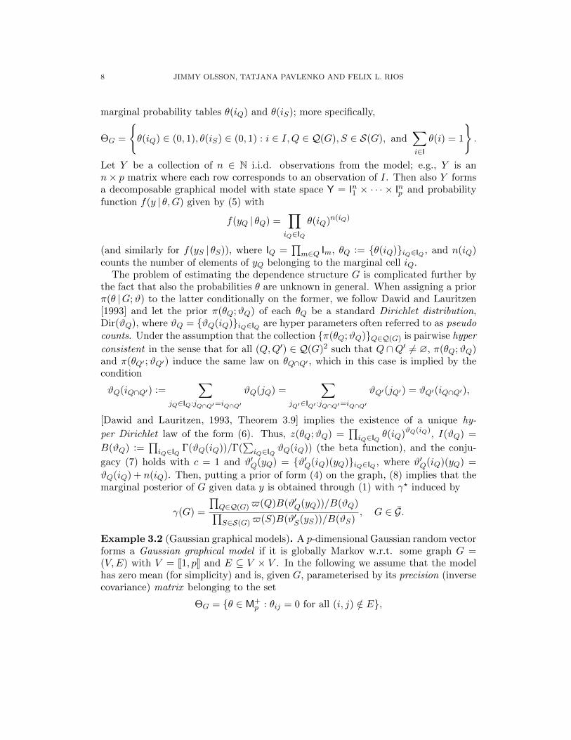
graph in Figure 2 with the estimated models in Figure 3, we observe that increasingN from 20 to 100 gives a slightly better agreement with the true adjacency matrix.This effect further can be explained by the behavior of the estimated autocorrelationfunction; by increasing N we observe a clear reduction of the autocorrelation. Quali-tatively we conclude that the mobility of the PG sampler is improved when increasingN .

6.3. Decomposable GGM with temporal dependence. In this example westudy a decomposable GGM where a temporal interpretation of the underlying de-pendence structure is sensible. The graph structure along with its adjacency matrixare displayed in Figure 4 and can be interpreted as an AR-process with lag vary-ing between 1 and 5. Regarding the parameterization, we consider the Gaussiandistribution with zero mean and covariance matrix θ−1 defined as

(θ−1)ij =

σ2, if i = j

ρσ2, if (i, j) ∈ G

and θij = 0 if (i, j) /∈ G. This is a modification of to the second order intra-classstructure considered in Thomas and Green [2009], but with varying band width. Weset σ = 1.0 and ρ = 0.9 and sampled n = 100 data vectors from this model. We usethe Hyper-Wishart prior for θ as described in Example 3.2 where for each clique Qthe shape parameter is set to be equal to p and the scale matrix v is set to be theidentity matrix of dimension |Q|.

The temporal interpretation of the dependence structure in the current exampleis as mentioned above particularly appealing for investigating the role of the neigh-borhood parameter δ. Estimation results are presented in Figure 5 and Figure 6.By comparing the two heatmaps one can see that the dependence structure can beefficiently captured by the proper choice of δ. Indeed, by selecting δ to be close to themaximal band size of 5 for the true graph and letting α = 0.8 and β = 0.5 reflectinga priority for connected graphs, we obtain a dependence pattern more similar to thetrue one. This is also reflected by the log-likelihood in the bottom row of Figure 6.On the other hand, in view of auto-correlation (after burn-in) shown in the middlerow of Figure 6, the mixing properties of the PG sampler seem to be improved byincreasing δ.

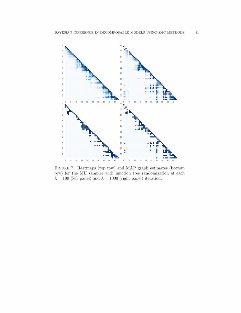
6.4. Comparison to Metropolis-Hasting sampler. As a reference, we compareour results from Section 6.3 to a Python implementation of the Metropolis-Hastings(MH) algorithm proposed in Thomas and Green [2009], where the model parametershave been marginalized out. The output is summarized in Figure 7 and Figure 8.In order to the mixing properties of the MH sampler we follow the suggestions ofThomas and Green [2009] and randomize the junction tree every λ iteration. Here,we show results for λ = 100 and λ = 1000 in the left and right columns of the figures,respectively.


1 2 3 4 5 6 7 8 9 10 11 12 13 14 15

15

14

13

12

11

10

9

8

7

6

5

4

3

2

1

1 2 3 4 5 6 7 8 9 10 11 12 13 14 15

15

14

13

12

11

10

9

8

7

6

5

4

3

2

1

0.0

0.2

0.4

0.6

0.8

1.0

1 2 3 4 5 6 7 8 9 10 11 12 13 14 15

15

14

13

12

11

10

9

8

7

6

5

4

3

2

1

1 2 3 4 5 6 7 8 9 10 11 12 13 14 15

15

14

13

12

11

10

9

8

7

6

5

4

3

2

1

0.0

0.2

0.4

0.6

0.8

1.0

0 2000 4000 6000 8000 10000Lag

−1.0

−0.5

0.0

0.5

1.0

Autoc

orrelatio

n

0 2000 4000 6000 8000 10000Lag

−1.0

−0.5

0.0

0.5

1.0

Autoc

orrelatio

n

Figure 3. Estimation of the graph posterior for the log-linear modelwith p = 15 and n = 100. The CTA parameters are α = 0.2, β = 0.8and δ = 15. The number of MCMC sweeps, M is set to 10000. Theleft and right panel correspond to N = 20 and N = 100 respec-tively. For both panels from top to bottom, the first figure presentsthe estimated edge heatmap, the estimated MAP graph and estimatedauto-correlation of the number of edges in the graph.


Firstly, we note that the estimated auto-correlation of the MH sampler shown inthe middle row of Figure 8, is substantially stronger than that for the PG samplerin both cases, being about 500 for δ = 50 compared to about 20000 for λ = 100.Also, from the size and the log-likelihood trajectory of the MH sampler presentedat the upper and lower row of Figure 8, respectively, the time to reach what seemslike a stationary distribution requires fewer steps in the PG sampler than for the MHsamples, being about 2000 for δ = 5 compared to about 350000 with λ = 100.

Both the heatmaps and MAP graphs for the MH sampler presented in Figure 7,confirm the suggestion of Thomas and Green [2009] that a more frequent junctiontree randomization in the MH sampler seems to have good effect on recovering theunderlying model.

6.5. Computational aspects. The main advantage for the MH sampler is the supe-rior speed, since it compensates for the inferior mixing properties seemingly inheritedby the local move approach. In this implementation, the 500000 iterations in the MHtook about 3 hours to generate, the acceptance rate were estimate to approximately0.03. For our non-optimized implementation of the PG sampler, each sample tookabout 7 seconds. However, we expect that the speed of the PG sampler could be im-proved by, for example employing more efficient data structures for the junction treerepresentation and by improved caching strategies. Note that in our implementation,no further advantage of the AR model has been taken when calculating the graphlikelihoods.

The Python program underlying this numerical study was executed on an iMaclate 2012 with 2.7 GHz Intel Core i5 processor. The code and evaluation datasetscan be obtained from the third author.

1

2

3

4

5

6

7

8

9

10

11

12

13

14

15

16

17

18

19

20

21

22

23

24

25

26

27

28

29

30

31

32

33

34

35

36

37

38

39

40

41

42

43

44

45

4647

48

49

50

1 2 3 4 5 6 7 8 910

11

12

13

14

15

16

17

18

19

20

21

22

23

24

25

26

27

28

29

30

31

32

33

34

35

36

37

38

39

40

41

42

43

44

45

46

47

48

49

50

5049484746454443424140393837363534333231302928272625242322212019181716151413121110987654321

Figure 4. The true underlying decomposable graph on p = 50 nodesalong with its adjacency matrix.


1 2 3 4 5 6 7 8 910

11

12

13

14

15

16

17

18

19

20

21

22

23

24

25

26

27

28

29

30

31

32

33

34

35

36

37

38

39

40

41

42

43

44

45

46

47

48

49

50

5049484746454443424140393837363534333231302928272625242322212019181716151413121110987654321

1 2 3 4 5 6 7 8 910

11

12

13

14

15

16

17

18

19

20

21

22

23

24

25

26

27

28

29

30

31

32

33

34

35

36

37

38

39

40

41

42

43

44

45

46

47

48

49

50

5049484746454443424140393837363534333231302928272625242322212019181716151413121110987654321

0.0

0.2

0.4

0.6

0.8

1.0

1 2 3 4 5 6 7 8 910

11

12

13

14

15

16

17

18

19

20

21

22

23

24

25

26

27

28

29

30

31

32

33

34

35

36

37

38

39

40

41

42

43

44

45

46

47

48

49

50

5049484746454443424140393837363534333231302928272625242322212019181716151413121110987654321

1 2 3 4 5 6 7 8 910

11

12

13

14

15

16

17

18

19

20

21

22

23

24

25

26

27

28

29

30

31

32

33

34

35

36

37

38

39

40

41

42

43

44

45

46

47

48

49

50

5049484746454443424140393837363534333231302928272625242322212019181716151413121110987654321

0.0

0.2

0.4

0.6

0.8

1.0

Figure 5. Heatmaps (top row) and MAP graph estimates (bottomrow) for the PG sampler with δ = 5 (left panel) and δ = 50 (rightpanel).


0 1000 2000 3000 4000 5000

150

200

250

300

350

400

0 1000 2000 3000 4000 5000

150

200

250

300

350

400

450

0 500 1000 1500 2000 2500 3000

Lag

−1.00

−0.75

−0.50

−0.25

0.00

0.25

0.50

0.75

1.00

Autocorrelation

0 500 1000 1500 2000 2500 3000

Lag

−1.00

−0.75

−0.50

−0.25

0.00

0.25

0.50

0.75

1.00

Autocorrelation

0 1000 2000 3000 4000 5000

1150

1200

1250

1300

1350

1400

1450

1500

0 1000 2000 3000 4000 5000

1000

1100

1200

1300

1400

1500

Figure 6. Size trajectory (top row), estimated size autocorrelation(middle row) and the graph log-likelihood (bottom row) for the PGsampler with δ = 5 (left panel) and δ = 50 (right panel).


0 5 10 15 20 25 30 35 40 45

4540

3530

2520

1510

50

0 5 10 15 20 25 30 35 40 45

4540

3530

2520

1510

50

0 5 10 15 20 25 30 35 40 45

4540

3530

2520

1510

50

0 5 10 15 20 25 30 35 40 45

4540

3530

2520

1510

50

Figure 7. Heatmaps (top row) and MAP graph estimates (bottomrow) for the MH sampler with junction tree randomization at eachλ = 100 (left panel) and λ = 1000 (right panel) iteration.


0 100000 200000 300000 400000 500000

0

50

100

150

200

250

0 100000 200000 300000 400000 500000

0

50

100

150

200

250

300

0 20000 40000 60000 80000 100000 120000 140000Lag

−1.00

−0.75

−0.50

−0.25

0.00

0.25

0.50

0.75

1.00

Autoc

orrelatio

n

0 20000 40000 60000 80000 100000 120000 140000Lag

−1.00

−0.75

−0.50

−0.25

0.00

0.25

0.50

0.75

1.00

Autoc

orrelatio

n

0 100000 200000 300000 400000 500000

−2000

−1000

0

1000

0 100000 200000 300000 400000 500000

−2500

−2000

−1500

−1000

−500

0

500

1000

1500

Figure 8. Size trajectories (top row), estimated size autocorrelations(middle row) and the graph log-likelihoods (bottom row) for the MHsampler with junction tree randomization at each λ = 100 (left panel)and λ = 1000 (right panel) iteration.


References

S. Byrne and A. P. Dawid. Structural Markov graph laws for Bayesian model uncer-tainty. Annals of Statistics, 43(4):1647–1681, 2015.

N. Chopin and S. S. Singh. On particle Gibbs sampling. Bernoulli, 21(3):1855–1883,08 2015.

R. Cowell, P. Dawid, S. Lauritzen, and D. Spiegelhalter. Probabilistic Networks andExpert Systems: Exact Computational Methods for Bayesian Networks. Informa-tion Science and Statistics. Springer New York, 2003.

T. H. David Edwards. A fast procedure for model search in multidimensional contin-gency tables. Biometrika, 72(2):339–351, 1985.

A. P. Dawid and S. L. Lauritzen. Hyper Markov laws in the statistical analysis ofdecomposable graphical models. The Annals of Statistics, 21(3):1272–1317, 1993.

P. Del Moral, A. Doucet, and A. Jasra. Sequential Monte Carlo samplers. Journalof the Royal Statistical Society. Series B (Statistical Methodology), 68(3):411–436,2006.

P. Dellaportas and J. J. Forster. Markov chain Monte Carlo model determination forhierarchical and graphical log-linear models. Biometrika, 86(3):615–633, 1999.

R. Diestel. Graph Theory. Number 173 in Graduate Texts in Mathematics. Springer,1997.

P. Giudici and P. J. Green. Decomposable graphical Gaussian model determination.Biometrika, 86(4):785–801, 1999.

P. J. Green and A. Thomas. Sampling decomposable graphs using a Markov chainon junction trees. Biometrika, 100(1):91–110, 2013.

B. Jones, C. Carvalho, A. Dobra, C. Hans, C. Carter, and M. West. Experiments instochastic computation for high-dimensional graphical models. Statistical Science,20(4):pp. 388–400, 2005.

S. L. Lauritzen. Graphical Models. Oxford University Press, 1996.D. Madigan and A. E. Raftery. Model selection and accounting for model uncertainty

in graphical models using Occam’s window. Journal of the American StatisticalAssociation, 89(428):1535–1546, 1994.

F. Maire, R. Douc, and J. Olsson. Comparison of asymptotic variances of inhomo-geneous Markov chains with application to Markov chain Monte Carlo methods.Ann. Statist., 42(4):1483–1510, 2014.

H. Massam, J. Liu, and A. Dobra. A conjugate prior for discrete hierarchical log-linearmodels. The Annals of Statistics, 37(6A):3431–3467, 2009.

C. O., E. Moulines, and T. Ryden. Inference in hidden Markov models. Springer NewYork, 2005.

J. Olsson, T. Pavlenko, and F. L. Rios. Generating junction trees of decomposablegraphs with the Christmas tree algorithm. ArXiv e-prints, 2017.

B. Rajaratnam, H. Massam, and C. M. Carvalho. Flexible covariance estimation ingraphical Gaussian models. The Annals of Statistics, 36(6):2818–2849, 2008.


T. P. Speed and H. T. Kiiveri. Gaussian Markov distributions over finite graphs. TheAnnals of Statistics, 14(1):138–150, 1986.

A. Thomas and P. J. Green. Enumerating the junction trees of a decomposable graph.Journal of Computational and Graphical Statistics, 18(4):930–940, 2009.

BAYESIAN INFERENCE IN DECOMPOSABLE GRAPHICAL MODELS …1141468/FULLTEXT01.pdf · MODELS USING...

Documents

Transcript of BAYESIAN INFERENCE IN DECOMPOSABLE GRAPHICAL MODELS …1141468/FULLTEXT01.pdf · MODELS USING...