Bayesian Graphical Models for Adaptive Filtering...Bayesian Graphical Models for Adaptive Filtering...
155
Bayesian Graphical Models for Adaptive Filtering Yi Zhang September 9, 2005 Language Technologies Institute School of Computer Science Carnegie Mellon University Pittsburgh, PA 15213 Thesis Committee: Jamie Callan, Chair (Carnegie Mellon University) Jaime Carbonell (Carnegie Mellon University) Thomas Minka (Microsoft Research Cambridge) Stephen Robertson (Microsoft Research Cambridge) Yiming Yang (Carnegie Mellon University) Copyright c 2004 Yi Zhang
Transcript of Bayesian Graphical Models for Adaptive Filtering...Bayesian Graphical Models for Adaptive Filtering...

Bayesian Graphical Models for Adaptive Filtering
Yi Zhang
September 9, 2005
Language Technologies Institute
School of Computer Science
Carnegie Mellon University
Pittsburgh, PA 15213
Thesis Committee:
Jamie Callan, Chair (Carnegie Mellon University)
Jaime Carbonell (Carnegie Mellon University)
Thomas Minka (Microsoft Research Cambridge)
Stephen Robertson (Microsoft Research Cambridge)
Yiming Yang (Carnegie Mellon University)
Copyright c© 2004 Yi Zhang

Abstract
A personal information filtering system monitors an incoming document stream to find the documents that
match information needs specified by user profiles. The most challenging aspect in adaptive filtering is to
develop a system to learn user profiles efficiently and effectively from very limited user supervision.
In order to overcome this challenge, the system needs to do the following: use a robust learning algorithm
that can work reasonably well when the amount of training data is small and be more effective with more
training data; explore what a user likes while satisfying the user’s immediate information need and trade
off exploration and exploitation; consider many aspects of a document besides relevance, such as novelty,
readability and authority; use multiple forms of evidence, such as user context and implicit feedback from
the user, while interacting with a user; and handle various scenarios, such as missing data, in an operational
environment robustly.
This dissertation uses the Bayesian graphical modelling approach as a unified framework for filtering.
We customize the framework to the filtering domain and develop a set of solutions that enable us to build a
filtering system with the desired characteristics in a principled way. We evaluate and justify these solutions
on a large and diverse set of standard and new adaptive filtering test collections. Firstly, we develop
a novel technique to incorporate an IR expert’s heuristic algorithm as a Bayesian prior into a machine
learning classifier to improve the robustness of a filtering system. Secondly, we derive a novel model quality
measure based on the uncertainty of model parameters to trade off exploration and exploitation and do
active learning. Thirdly, we carry out a user study with a real web-based personal news filtering system and
more than 20 users. With the data collected in the user study, we explore how to use existing graphical
modeling algorithms to learn the causal relationships between multiple forms of evidence and improve the
filtering system’s performance using this evidence.
i

Acknowledgements
First and foremost, I would like to thank my advisor, Jamie Callan, for all the support over the last six years.
Jamie is a great advisor who has given me the perfect combination of technical advice and research freedom.
From him, I have learned how to conduct serious research to provide realistic solutions to real problems, I
have learned how to collaborate with other people and share the success, I have learned how to improve my
technical speaking and writing, and much more. Jamie, thank you for your guidance on this research topic,
on research methodology and life in general.
I am grateful to the other members of my committee, Yiming Yang, Jaime Carbonell, Thomas Minka and
Stephen Robertson. They proved to be the most thorough reviewers, as I expected. They have helped me
better focus my dissertation and have kept me accurate about all the details. Yiming has been very helpful
ever since the time I started my life in CMU. She has provided very useful general advise on how to conduct
research, detailed support on TDT evaluation, and much useful feedback on the LR Rocchio algorithm.
Jaime has provided many concrete suggestions on how to improve the presentation of the dissertation as
well as numerous valuable comments on the technical details. I appreciate Thomas Minka for his ability to
understand several important issues in this dissertation (even when I didn’t really understand them myself).
I am grateful to Steve for helping me design the user study, for better positioning the contribution of the
dissertation for the information retrieval community, and for identifying several important issues I would
have missed.
I am very glad that I have had the chance to study at the Language Technology Institute in School
of Computer Science, Carnegie Mellon University. The open and friendly environment in CMU make it a
wonderful place for research. I have benefit tremendously from interactions with faculty, friends, and fellow
students. I am grateful to all them. I especially would like to mention Kevyn Collins-Thompson, Peter
Spirtes, Jian Zhang, John Lafferty, Zoubin Ghahramani, Roni Rosenfeld, Chengxiang Zhai, Fan Li, Shinjae
Yoo, Bryan Kisiel, Nianli Ma, Si Luo, Jerry Zhu, Thi Nhu Truong, Ricardo Silva, Scott Fahlman, Jiji Zhang,
Paul Bennett, Isa Verdinelli, Rong Yan, Yan Liu, Weng-Keen Wong, Andrew Moore, and Paul Komarek. I
especially would like to thank Paul Ogilvie for being a wonderful officemate. Paul has carefully proofread
my papers, including the last version of my dissertation, which helped to improve the presentations a lot.
Thanks to many people from outside CMU with whom I have had valuable discussions of ideas related to
ii

Acknowledgements iii
this dissertation. Thanks to Joemon Jose and Susan Dumais for valuable discussions. Thank to Diane Kelly
for suggestions on how to run the user study. Thank to David Hull, Jimi Shanahan, David Evans for the
comments on the thesis proposal. Thank to James Allan for supporting my trip to TDT workshop. Thank
to Wensi Xi for working with me on developing another news filtering system. I would also like to thank
Byron Dom, Shivakumar Vaithyanathan, and other researchers I collaborated with at IBM Almaden research
center - Iris Eiron, Ashutosh Garg, Huayu Zhu, Alex Cozzi, Hongxia Jin, Philip Beineke and William Cody
- for the fun and valuable intern experience. I am also grateful for the IBM fellowship I received in the last
two years, which allowed me to focus on my research.
I am grateful to all my friends with whom I have spent the six years in Pittsburgh. In particular, I
want to thank my roommates Qin Jin, Tao Chen, Yan Lu, Lv Yong and Peng Chang for providing the fun
distractions from the school.
I owe a great deal to my parents who gave a life and endless love to me. They have worked very hard to
provide me the opportunity to receive the best possible education in China. They have influenced me with
their desire to learn, love for sharing and the optimistic attitude, which I will benefit from forever.
I am deeply indebted to my dear husband Wei for his love, encouragement and tremendous support for
my graduate study. Without him, it is impossible for me to finish this six years of long journey. Wei, you
gave me the motivation to finish this thesis and it is dedicated to you.

To Wei
&
my parents
iv

Contents
1 Introduction 1
1.1 What is filtering . . . . . . . . . . . . . . . . . . . . . . . . . . . . . . . . . . . . . . . . . . . 1
1.2 Bayesian graphical models for adaptive filtering . . . . . . . . . . . . . . . . . . . . . . . . . . 2
1.3 The goal of this dissertation and overview of the solutions . . . . . . . . . . . . . . . . . . . . 5
1.4 Contributions of the dissertation . . . . . . . . . . . . . . . . . . . . . . . . . . . . . . . . . . 6
1.5 Outline . . . . . . . . . . . . . . . . . . . . . . . . . . . . . . . . . . . . . . . . . . . . . . . . 8
2 Literature Review and Background Knowledge 9
2.1 Adaptive filtering standards . . . . . . . . . . . . . . . . . . . . . . . . . . . . . . . . . . . . . 9
2.1.1 Evaluation measures . . . . . . . . . . . . . . . . . . . . . . . . . . . . . . . . . . . . . 10
2.1.2 Evaluation data sets . . . . . . . . . . . . . . . . . . . . . . . . . . . . . . . . . . . . . 13
2.2 Existing retrieval models and filtering approaches . . . . . . . . . . . . . . . . . . . . . . . . . 16
2.2.1 Existing retrieval models . . . . . . . . . . . . . . . . . . . . . . . . . . . . . . . . . . 16
2.2.2 Existing adaptive filtering approaches . . . . . . . . . . . . . . . . . . . . . . . . . . . 19
2.3 Bayesian Graphical Models . . . . . . . . . . . . . . . . . . . . . . . . . . . . . . . . . . . . . 20
2.3.1 Bayes’ theorem . . . . . . . . . . . . . . . . . . . . . . . . . . . . . . . . . . . . . . . . 21
2.3.2 Graphical models . . . . . . . . . . . . . . . . . . . . . . . . . . . . . . . . . . . . . . . 22
2.3.3 Algorithms for structure learning . . . . . . . . . . . . . . . . . . . . . . . . . . . . . . 25
2.3.4 Algorithms for probabilistic inference . . . . . . . . . . . . . . . . . . . . . . . . . . . . 27
2.3.5 Bayesian experimental design and sequential decision problem . . . . . . . . . . . . . . 29
3 Integrating Expert’s Heuristics using Bayesian Priors 32
3.1 Existing algorithms . . . . . . . . . . . . . . . . . . . . . . . . . . . . . . . . . . . . . . . . . . 33
3.1.1 Rocchio algorithm . . . . . . . . . . . . . . . . . . . . . . . . . . . . . . . . . . . . . . 34
3.1.2 Logistic regression . . . . . . . . . . . . . . . . . . . . . . . . . . . . . . . . . . . . . . 35
3.2 New algorithm: LR Rocchio . . . . . . . . . . . . . . . . . . . . . . . . . . . . . . . . . . . . . 37
3.3 Experimental methodology . . . . . . . . . . . . . . . . . . . . . . . . . . . . . . . . . . . . . 39
v

vi CONTENTS
3.4 Experimental results . . . . . . . . . . . . . . . . . . . . . . . . . . . . . . . . . . . . . . . . . 40
3.5 Related work and further discussion . . . . . . . . . . . . . . . . . . . . . . . . . . . . . . . . 46
3.6 Summary . . . . . . . . . . . . . . . . . . . . . . . . . . . . . . . . . . . . . . . . . . . . . . . 48
4 Exploration and Exploitation Trade-off using Bayesian Active Learning 50
4.1 Algorithm . . . . . . . . . . . . . . . . . . . . . . . . . . . . . . . . . . . . . . . . . . . . . . . 51
4.1.1 Exploitation using Bayesian inference . . . . . . . . . . . . . . . . . . . . . . . . . . . 53
4.1.2 Exploration using Bayesian active learning . . . . . . . . . . . . . . . . . . . . . . . . 53
4.1.3 Determining the dissemination threshold based on logistic regression . . . . . . . . . . 56
4.1.4 Computational issues . . . . . . . . . . . . . . . . . . . . . . . . . . . . . . . . . . . . 57
4.2 Experimental methodology . . . . . . . . . . . . . . . . . . . . . . . . . . . . . . . . . . . . . 59
4.3 Experimental results . . . . . . . . . . . . . . . . . . . . . . . . . . . . . . . . . . . . . . . . . 60
4.4 Related work and our contributions . . . . . . . . . . . . . . . . . . . . . . . . . . . . . . . . . 62
4.5 Summary . . . . . . . . . . . . . . . . . . . . . . . . . . . . . . . . . . . . . . . . . . . . . . . 64
5 User Study 66
5.1 System description . . . . . . . . . . . . . . . . . . . . . . . . . . . . . . . . . . . . . . . . . . 66
5.2 Subjects . . . . . . . . . . . . . . . . . . . . . . . . . . . . . . . . . . . . . . . . . . . . . . . . 69
5.3 Data collected . . . . . . . . . . . . . . . . . . . . . . . . . . . . . . . . . . . . . . . . . . . . . 70
5.3.1 Explicit user feedbacks . . . . . . . . . . . . . . . . . . . . . . . . . . . . . . . . . . . . 70
5.3.2 User actions (Implicit feedback) . . . . . . . . . . . . . . . . . . . . . . . . . . . . . . . 71
5.3.3 Topic information . . . . . . . . . . . . . . . . . . . . . . . . . . . . . . . . . . . . . . 71
5.3.4 News Source Information . . . . . . . . . . . . . . . . . . . . . . . . . . . . . . . . . . 72
5.3.5 Content of each document . . . . . . . . . . . . . . . . . . . . . . . . . . . . . . . . . . 72
5.4 Preliminary data analysis . . . . . . . . . . . . . . . . . . . . . . . . . . . . . . . . . . . . . . 73
5.4.1 Basic statistics . . . . . . . . . . . . . . . . . . . . . . . . . . . . . . . . . . . . . . . . 73
5.4.2 Correlation analysis . . . . . . . . . . . . . . . . . . . . . . . . . . . . . . . . . . . . . 77
5.4.3 User specific analysis . . . . . . . . . . . . . . . . . . . . . . . . . . . . . . . . . . . . . 78
5.4.4 Comparison with Claypool’s user study . . . . . . . . . . . . . . . . . . . . . . . . . . 78
5.5 Summary . . . . . . . . . . . . . . . . . . . . . . . . . . . . . . . . . . . . . . . . . . . . . . . 83
6 Combining Multiple Forms of Evidence Using Graphical Models 85
6.1 Understanding the domain using causal structure learning . . . . . . . . . . . . . . . . . . . . 86

CONTENTS vii
6.2 Improving system performance using inference algorithms . . . . . . . . . . . . . . . . . . . . 94
6.2.1 Experimental Design . . . . . . . . . . . . . . . . . . . . . . . . . . . . . . . . . . . . . 94
6.2.2 Experimental results and discussions . . . . . . . . . . . . . . . . . . . . . . . . . . . . 99
6.3 Related work and further discussion . . . . . . . . . . . . . . . . . . . . . . . . . . . . . . . . 106
6.4 Future work . . . . . . . . . . . . . . . . . . . . . . . . . . . . . . . . . . . . . . . . . . . . . . 109
6.4.1 User specific models for inference . . . . . . . . . . . . . . . . . . . . . . . . . . . . . . 109
6.4.2 Better models for inference . . . . . . . . . . . . . . . . . . . . . . . . . . . . . . . . . 110
6.4.3 Integrating novelty/redundancy and authority estimations into graphical models . . . 111
6.5 Summary . . . . . . . . . . . . . . . . . . . . . . . . . . . . . . . . . . . . . . . . . . . . . . . 112
7 Conclusion and future work 115
7.1 Contributions . . . . . . . . . . . . . . . . . . . . . . . . . . . . . . . . . . . . . . . . . . . . . 115
7.1.1 General contribution: A theoretical framework . . . . . . . . . . . . . . . . . . . . . . 116
7.1.2 Specific contributions . . . . . . . . . . . . . . . . . . . . . . . . . . . . . . . . . . . . 117
7.1.3 Contribution beyond filtering . . . . . . . . . . . . . . . . . . . . . . . . . . . . . . . . 119
7.2 Limitation and future directions . . . . . . . . . . . . . . . . . . . . . . . . . . . . . . . . . . 119
7.2.1 Computationally efficient techniques . . . . . . . . . . . . . . . . . . . . . . . . . . . . 120
7.2.2 User independent, user specific, and cluster specific models . . . . . . . . . . . . . . . 120
7.2.3 Temporal property of adaptive filtering . . . . . . . . . . . . . . . . . . . . . . . . . . 121
7.2.4 Automatically testing of assumptions . . . . . . . . . . . . . . . . . . . . . . . . . . . . 122
8 Appendix 124
8.1 Appendix 1: Terminologies . . . . . . . . . . . . . . . . . . . . . . . . . . . . . . . . . . . . . 124
8.2 Appendix 2: Exit Questionnaire . . . . . . . . . . . . . . . . . . . . . . . . . . . . . . . . . . . 125

List of Figures
1.1 A typical filtering system. . . . . . . . . . . . . . . . . . . . . . . . . . . . . . . . . . . . . . 3
2.1 A graphical model for relevance filtering. . . . . . . . . . . . . . . . . . . . . . . . . . . . . . . 21
2.2 The representation of plate. The diagram on the left is a different representation for the
graphical model on the right. The shorthand representation on the left means variables Xt
are conditionally independent and identically distributed given φ. . . . . . . . . . . . . . . . . 24
2.3 A graphical model representation for logistic regression or linear regression. . . . . . . . . . . 24
2.4 An example of directed acyclic graph with five nodes. . . . . . . . . . . . . . . . . . . . . . . 24
2.5 An undirected graph: (A,D,C), (C,B), and (D,E,C) are cliques. . . . . . . . . . . . . . . . . . 24
3.1 Comparison of the performance on individual profile: T11U of Logistic Rocchio - T11U of
LogisticRegression. . . . . . . . . . . . . . . . . . . . . . . . . . . . . . . . . . . . . . . . . . . 42
3.2 Comparison of the performance on individual profile: T11U of Logistic Rocchio - T11U of
Rocchio. . . . . . . . . . . . . . . . . . . . . . . . . . . . . . . . . . . . . . . . . . . . . . . . . 42
3.3 Comparison with other TREC participants. The T11SU values of different runs on the TREC-
11 adaptive filtering task are reported in this figure. Systems in the legend from top to bottom
correspond to bars from left to right. Our results and the results of TREC-11 participants
are not directly comparable, because we have had greater experience with the dataset. The
figure is provided only to give context for the results reported in this dissertation. . . . . . . . 43
3.4 A comparison of the performance of different profile learning algorithms over time on the
TREC-11 adaptive filtering task. This figure is the average of 50 user profiles. . . . . . . . . . 44
4.1 Exploitation and exploration for relevance filtering. Step 1: Messages are passed from known
nodes “θ” and “dt” to “relevant” to estimate the probabilistic distribution of “relevant”. Then
we can estimate the immediate utility. Step 2: Messages are passed from known nodes “dt”
and “relevant” to unknown node “θ” to estimate the probabilistic distribution of “θ”, assuming
we know the relevance feedback about document “dt”. Then we estimate the future utility
gain if dt is delivered, based on the probabilistic distribution of parameter “θ”. . . . . . . . . 52
viii

LIST OF FIGURES ix
4.2 Comparison of the performance of threshold-learning algorithms over time on the TREC-10
filtering data. . . . . . . . . . . . . . . . . . . . . . . . . . . . . . . . . . . . . . . . . . . . . . 60
5.1 The user study system structure. The structured information, such as user feedback and
crawler statistics, is kept in the database. The content of each web page crawled is saved in
the news repository. . . . . . . . . . . . . . . . . . . . . . . . . . . . . . . . . . . . . . . . . . 67
5.2 Web interface after a user logs in. . . . . . . . . . . . . . . . . . . . . . . . . . . . . . . . . . . 68
5.3 The interface for users to provide explicit feedback on the current news story. . . . . . . . . . 69
5.4 The number of classes each user has created. . . . . . . . . . . . . . . . . . . . . . . . . . . . 74
5.5 The histogram of the number of documents the 28 users clicked and evaluated for each class. 75
5.6 The histogram of the number of documents user clicked and evaluated for each class: X
truncated to 25. . . . . . . . . . . . . . . . . . . . . . . . . . . . . . . . . . . . . . . . . . . . . 75
5.7 The histogram of four different explicit user feedback. -1 means the user didn’t provide the
feedback. relevant and novel are recorded as integers ranging from 1 (least) to 5 (most).
readable and authoritative are recorded as 0(negative) or 1(positive). . . . . . . . . . . . . . . 80
5.8 The histogram of milliseconds spent on a page. . . . . . . . . . . . . . . . . . . . . . . . . . . 81
5.9 The histogram of more variables: user likes, and topic like. . . . . . . . . . . . . . . . . . . . 81
5.10 Multiple comparison of the average time (in milliseconds) spent on a page for different users.
Only 17 users with more than 200 feedback entries are included. Most of the users spent less
than 100 seconds/page on average. . . . . . . . . . . . . . . . . . . . . . . . . . . . . . . . . . 82
5.11 Multiple comparison of the average number of up arrow (↑) usage on a page for different users.
Only 17 users with more than 200 feedback entries are included. . . . . . . . . . . . . . . . . 82
5.12 Multiple comparison of the average number of down arrow (↓) on a page for different users.
Only 17 users with more than 200 feedback entries are included. . . . . . . . . . . . . . . . . 82
5.13 Multiple comparison of the average user likes rating for different users. Only 17 users with
more than 200 feedback entries are included. . . . . . . . . . . . . . . . . . . . . . . . . . . . 82
6.1 Prior knowledge as temporal tier of variables before automatic structure learning. This prior
knowledge informs the learning algorithm that a causation (indicated by→) from a higher level
to lower level, such as relevant is a direct or indirect cause of RSS info (relevant→ RSSInfo),
is prohibited. . . . . . . . . . . . . . . . . . . . . . . . . . . . . . . . . . . . . . . . . . . . . . 88

x LIST OF FIGURES
6.2 A user independent causal graphical structure learned using PC algorithm. The learning
algorithm begins with the 5 tier prior knowledge. In the causal graph, X − Y means the
algorithm cannot tell if X causes Y or if Y causes X. X ←→ Y means the algorithm found
some problem. The problem may happen because of a latent common cause of X and Y, a
chance pattern in a sample, or other violations of assumptions. . . . . . . . . . . . . . . . . . 89
6.3 A user independent causal graphical structure learned using PC algorithm. The learning
algorithm begins with the 2 tier prior knowledge. . . . . . . . . . . . . . . . . . . . . . . . . . 90
6.4 A user independent causal graphical structure learned using FCI algorithm. The learning
algorithm begins with the 5 tier prior knowledge. X → Y means X is a direct or indirect
cause of Y. X ↔ Y means there is an unrecorded common cause of X and Y. “o” means the
algorithm cannot determine whether there should or should not be an arrowhead at that edge
end. An edge from X to Y that has an arrowhead directed into Y means Y is not a direct or
undirect cause of X. . . . . . . . . . . . . . . . . . . . . . . . . . . . . . . . . . . . . . . . . . 91
6.5 Graph structure for GM complete. In these graphs, RSS info={RSS link, host link} and Topic
info={familiar topic before, topic like} are 2 dimensional vectors representing the information
about the news source and the topic in Table 5.5 and Table 5.4. actions=<TimeOnPage,...>
is a 12 dimensional vector representing the user actions in Table 5.2. user likes is the target
variable the system predicts. . . . . . . . . . . . . . . . . . . . . . . . . . . . . . . . . . . . . 95
6.6 Graph structure for GM causal. . . . . . . . . . . . . . . . . . . . . . . . . . . . . . . . . . . . 96
6.7 Graph structure for GM inference. . . . . . . . . . . . . . . . . . . . . . . . . . . . . . . . . . 96
6.8 Comparison of the prediction power of different models: forms of evidence ordered by corre-
lation coefficient. From left to right, additional sources of evidence are given when testing.
“+RSS info” means the values of news source information (RSS info) are given besides the
value of relevance score, Topic Info, and readability score. . . . . . . . . . . . . . . . . . . . . 100
6.9 Comparison of the prediction power of GM complete at different missing evidence conditions:
forms of evidence ordered by user effort involved. . . . . . . . . . . . . . . . . . . . . . . . . . 100
6.10 Comparison of the prediction power of different graphical models: forms of evidence ordered
by correlation coefficient. . . . . . . . . . . . . . . . . . . . . . . . . . . . . . . . . . . . . . . 103
7.1 User specific and user independent models . . . . . . . . . . . . . . . . . . . . . . . . . . . . . 121
7.2 Cluster based user models. . . . . . . . . . . . . . . . . . . . . . . . . . . . . . . . . . . . . . . 122
List of Tables
2.1 The values assigned to relevant and non-relevant documents that the filtering system did and
did not deliver. R−, R+, N+ and N− correspond to the number of documents that fall into
the corresponding category. AR, AN , BR and BN correspond to the credit/penalty for each
element in the category. . . . . . . . . . . . . . . . . . . . . . . . . . . . . . . . . . . . . . . . 11
2.2 PC algorithm. . . . . . . . . . . . . . . . . . . . . . . . . . . . . . . . . . . . . . . . . . . . . . 26
3.1 A comparison of different algorithms on the TREC-9 OHSUMED data set. . . . . . . . . . . 40
3.2 A comparison of different algorithms on the TREC-11 Reuter’s data set. . . . . . . . . . . . 41
3.3 A comparison of different algorithms on the TREC-11 Reuter’s data set using the old relevance
judgments. . . . . . . . . . . . . . . . . . . . . . . . . . . . . . . . . . . . . . . . . . . . . . . 41
3.4 The utilities of submitted supervised adaptation topic tracking results reported by NIST.
CMU7 and CMU8 are our runs. Besides us, three other teams submitted their results of
several runs. . . . . . . . . . . . . . . . . . . . . . . . . . . . . . . . . . . . . . . . . . . . . . 45
3.5 A comparison of logistic regression (LR) with Logistic Rocchio on the TDT5 Multilingual
data set. . . . . . . . . . . . . . . . . . . . . . . . . . . . . . . . . . . . . . . . . . . . . . . . . 46
4.1 Pseudo code for determining a threshold. . . . . . . . . . . . . . . . . . . . . . . . . . . . . . 58
4.2 Comparison of four threshold-learning algorithms on the TREC-10 filtering data (Reuter’s
data set). . . . . . . . . . . . . . . . . . . . . . . . . . . . . . . . . . . . . . . . . . . . . . . . 60
4.3 Comparison of Bayesian active learning and Bayesian immediate learning on one user profile. 61
4.4 Comparison of the threshold learning algorithms on the TREC-9 filtering data set (OHSUMED
data, OHSU topics). . . . . . . . . . . . . . . . . . . . . . . . . . . . . . . . . . . . . . . . . . 61
5.1 Samples of class labels provided by the users and the number of documents put in each class. 76
5.2 Basic descriptive statistics about explicit feedbacks. RLO and RUP are the lower and upper
bounds for a 95% confidence interval for each coefficient. . . . . . . . . . . . . . . . . . . . . . 79
5.3 Basic descriptive statistics about user actions. The unit for TimeOnPage and TimeOnMouse
is millisecond. . . . . . . . . . . . . . . . . . . . . . . . . . . . . . . . . . . . . . . . . . . . . . 79
xi

xii LIST OF TABLES
5.4 Basic descriptive statistics about topics. . . . . . . . . . . . . . . . . . . . . . . . . . . . . . . 79
5.5 Basic descriptive statistics about news sources. RSS LINK is the number of web pages that
link to the RSS source. HOST LINK is the number of pages that link to the server of the
RSS source. . . . . . . . . . . . . . . . . . . . . . . . . . . . . . . . . . . . . . . . . . . . . . . 79
5.6 Basic descriptive statistics about documents. The length of the document does not include
HTML tags. . . . . . . . . . . . . . . . . . . . . . . . . . . . . . . . . . . . . . . . . . . . . . . 79
5.7 Basic descriptive statistics about user actions collected by the system used in [37]. corr is the
correlation coefficient between each form of evidence and the explicit feedback on [37]’s data.
corrYow is the correlation coefficient between each form of evidence and the explicit feedback
user likes on our user study data. . . . . . . . . . . . . . . . . . . . . . . . . . . . . . . . . . . 83
6.1 The correlation coefficient between explicit feedback. . . . . . . . . . . . . . . . . . . . . . . . 93
6.2 The values assigned to documents with different user likes ratings. A1, A2, A3, A4, and A5 cor-
respond to the number of documents that fall into the corresponding category. C1, C2, C3, C4
and C5 correspond to the credit/penalty for each element in the category. . . . . . . . . . . . 101
6.3 A comparison of effect of adding user actions. “relevance score”, “readability score”, “RSS
info” and “topic info” are given before actions where added. The data entries with missing
value are also used for training and testing. corr is the correlation coefficient between the
predicted value of user likes using the model and the true explicit feedback provided by the
users. RLO and RUP are the lower and upper bounds for a 95% confidence interval for each
coefficient. . . . . . . . . . . . . . . . . . . . . . . . . . . . . . . . . . . . . . . . . . . . . . . . 103
6.4 A comparison of different models: no missing value cases, coefficient measure. RLO and RUP
are the lower and upper bounds for a 95% confidence interval for each coefficient. . . . . . . . 105
6.5 A comparison of different models: all cases, utility measure. If we deliver all documents in
the testing data to the user, the utility is 2881.5. The highest possible utility on the testing
data is 3300. . . . . . . . . . . . . . . . . . . . . . . . . . . . . . . . . . . . . . . . . . . . . . 106
6.6 Comparing user specific models with user independent model for some users. “corr” is the
correlation coefficient between the predicted value of user likes using the model and the true
explicit feedback provided by the users. “Train No.” is the number of training documents
used to learn each model. RLO and RUP are the lower and upper bounds for a 95% confidence
interval for each coefficient. . . . . . . . . . . . . . . . . . . . . . . . . . . . . . . . . . . . . . 110

Chapter 1
Introduction
1.1 What is filtering
An agent working in the Homeland Security Department wants to be alerted of any information related to
potential terror attacks; a customer call center representative wants the phone routing system to route a
customer call reporting a specific product problem to him if the problem matches his expertise; a student
wants to be alerted of fellowship or financial aid opportunities appropriate for her/his circumstances; and a
financial analyst wants to be alerted of any information that may affect the price of the stock he is tracking.
In these examples, the user preferences are comparatively stable and represent a long term information
need, the information source is dynamic, information arrives sequentially over time, and the information
needs to be delivered to the user as soon as possible. Traditional ad hoc search engines, which are designed
to help the users to pull out information from a comparatively static information source, are inadequate to
fulfill the requirements of these tasks. Instead, a filtering system can serve the user better. A filtering system
is an autonomous agent that delivers good information to the user in a dynamic environment. As opposed
to forming a ranked list, it estimates whether a piece of information matches the user needs as soon as the
information arrives and pushes the information to the user if the answer is “yes”. So a user can be alerted
of any important information on time.
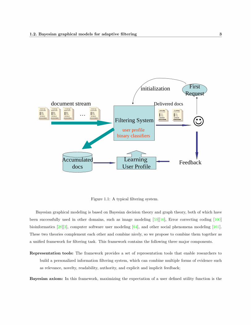
A typical information filtering system is shown in Figure 1.1.∗ In this figure, a piece of information is a
document.† A user’s information needs are represented in a user profile. The profile contains one or more
classes, such as “stock” or “music”, and each class corresponds to one information need. When a user has
a new information need, he/she sends to the system an initial request, such as a query or some sample
documents of what he/she wants. Then the system initializes and creates a new online classifier in the user’s
profile to serve this information need. As more future documents arrive, the system delivers documents the
classifier considered good to the user. The user may read delivered documents and provide explicit feedback,
∗A filtering system can serve many users, although only one user is shown in the figure.†Information can be documents, images, or videos. This dissertation focuses on documents.
1

2 Chapter 1. Introduction
such as identifying a document as “good” or “bad”. The user also provides some implicit feedback, such as
deleting a document without reading it or saving a document. The filtering system uses the user feedback
accumulated over time to update the user profile and classifiers frequently.
Standard ad hoc retrieval systems, such as search engines, let user use short queries to pull out information
and treat users the same given the query words. However, users are different and are not good at describing
their information needs using ad hoc queries. If the information need of a user is more or less stable over a
long period of time, a filtering system has a good environment to learn user profiles (also called user models)
from a fair amount of user feedback that can be accumulated over time. In other words, the system can
serve the user better by learning user profiles while interacting with the user, thus information delivered to
the user can be personalized and catered to individual user’s information needs automatically. Even if the
user’s interest drifts or changes, the system can still adapt to the user’s new interest by constantly updating
the user profile from training data, creating new classes automatically [50], or letting the user create/delete
classes.
While learning user profiles is an advantage of a filtering system, it is also a major research challenge
in the adaptive filtering research community. Common learning algorithms require a significant amount of
training data. However, a real-world filtering system must work as soon as the user uses the system, when
the amount of training is extremely small or zero. ‡ How should a good filtering system learn user profiles
efficiently and effectively with limited user supervision while filtering? In order to solve this problem, the
system needs to do the following efficiently: use a robust learning algorithm that can work reasonably well
when the amount of training data is small and more effective with more training data; explore what the user
likes while satisfying a user immediate information need and trade off exploration and exploitation; consider
many aspects of a document besides relevance, such as novelty, readability and authority; use multiple forms
of evidence, such as user context and implicit feedback from the user, while interacting with a user; and
handle various scenarios, such as missing data, robustly.
1.2 Bayesian graphical models for adaptive filtering
We hypothesize that Bayesian graphical modelling (BGM) is a useful and unified framework to guide us
building a filtering system with the above desired characteristics in a principled way. This dissertation tests
the hypothesis and studies how to customize the Bayesian graphical modelling approach into the filtering
domain to build filtering systems with the desired characteristics.
‡It is possible the system needs to begin working given a short user query and no positive instance.
1.2. Bayesian graphical models for adaptive filtering 3
Filtering System…
Accumulateddocs
document stream Delivered docs
FeedbackLearning
User Profile
☺
FirstRequest
initialization
user profile binary classifiers
Figure 1.1: A typical filtering system.
Bayesian graphical modeling is based on Bayesian decision theory and graph theory, both of which have
been successfully used in other domains, such as image modeling [59][16], Error correcting coding [100]
bioinformatics [28][3], computer software user modeling [64], and other social phenomena modeling [101].
These two theories complement each other and combine nicely, so we propose to combine them together as
a unified framework for filtering task. This framework contains the following three major components.
Representation tools: The framework provides a set of representation tools that enable researchers to
build a personalized information filtering system, which can combine multiple forms of evidence such
as relevance, novelty, readability, authority, and explicit and implicit feedback;
Bayesian axiom: In this framework, maximizing the expectation of a user defined utility function is the

4 Chapter 1. Introduction
only decision criterion;
Inference tools: Statistical inference algorithms introduced in Section 2.3.4 are the tools that enable us to
estimate probability distributions that can be used to achieve the goal of maximizing the utility.
Compared with other commonly used text classification algorithms, the proposed framework has five
major advantages.
First, the goal of a system is clearly defined in a broader way. Most filtering systems only optimize for
a very narrow definition of topical relevance, while we want to optimize for a broader, more realistic set of
criteria that can be expressed as a utility function. This utility function is defined based on whether the
user likes a document or not, and can be influenced by relevance,§ novelty, authority and readability of a
document. It is very natural to understand and optimize this utility function according to the Bayesian
axiom.
Second, the filtering system models the uncertainty explicitly using probabilities. Researchers in the
information retrieval community often estimate the uncertainty of relevance, and talk about the uncertainty
about a user profiles. However, the uncertainty about a user profile is not modeled explicitly. Existing
filtering systems usually use a point estimator of the parameter, such as maximum likelihood estimation or
max posterior estimation, to make predictions and decisions. In the Bayesian framework, the uncertainty
about a user profile is modeled explicitly as a probabilistic distribution of model parameters, and the filtering
system can estimate a user profile quality and do active learning based on the distribution.
Third, the framework helps us to understand the causal relationships in the domain and further improve
the design of the filtering system. For example, knowing whether a user likes a document may cause the user
to spend more time reading the document can help the system designer decide whether to collect the time
spent on a page as an implicit feedback. Understanding the causal relationships can also help us to predict
the consequences of intervention. For example, we may want to know if system gives a document a high
score, whether the user’s rating of the document will be influenced. The representation tools, especially the
causal structure learning algorithm, can help us to answer these questions.
Fourth, the framework enables us to combine prior domain knowledge or heuristics with training data.
Prior domain knowledge or heuristics are very important when the training data is scarce or expensive to
get. Bayes’ theorem makes it natural to encode this information as a prior distribution of the parameter
§The word “relevant” was used ambiguously, either as a narrow definition of “related to the matter at hand (aboutness)” ora broader definition of “having the ability to satisfy the needs of the user”. When it is used by the second definition, researcherswere usually studying what this dissertation refers to as user likes. In this dissertation, we use “relevant” as is defined in thefirst definition and use the phrase “user likes” for the second definition.

1.3. The goal of this dissertation and overview of the solutions 5
to be estimated, and graph structure learning algorithms also provide the mechanism to encode the prior
knowledge for the task of causal discovery (Section 2.3.3).
Fifth, the framework handles situations of missing data naturally based on the conditional dependencies
encoded in the graph structure. The unpredictability of user behaviors and system glitches make it difficult
to collect all the information one intends to collect. Training data with missing entries is very common in the
real world, and a robust system needs to learn and make predictions with partial observations. In the BGM
framework, missing data means some nodes are hidden. The inference tools discussed in detail in Section
2.3.4 can estimate the conditional probability of unknown nodes given whatever known.
With the above five advantages, we hypothesize Bayesian graphical modelling is a good unified framework
to guide us developing a filtering system with the desired characteristics and solve the limited training data
problem.
1.3 The goal of this dissertation and overview of the solutions
The Bayesian graphical modeling framework is not a universal solution to all filtering problems. Instead, it
is a set of general tools and design principles. Knowing the functionalities provided by the tools and a good
understanding of the filtering problem domain are both important in order to build a good filtering system
under the framework.
The goal of this dissertation is to explore how to customize Bayesian graphical models to the task of
filtering and help solve the limited user supervision problem (limited training data).
The approach we take is considering what humans may do to solve the same filtering problem, identifying
desirable characteristics of a filtering system motivated from humans, and then developing solutions that
enable the system to behave as desired using tools or principles provided by the Bayesian graphical modeling
framework.
First, humans may solve the problem by consulting with domain experts and using heuristics. Motivated
by this, we use simple heuristic models developed by an IR expert to influence the learning of statistical
models using a Bayesian prior.
Second, humans may do active learning by carefully picking the right document to ask the user for
feedback so that the answer can provide the most valuable information. Motivated by this, we measure the
utility gain of delivering a document (asking the user for feedback) explicitly based on Bayesian decision
theory. Using this measure, exploitation (making the user happy right now) and exploration (asking the user
for feedback) can be combined in a unified framework to optimize a user utility function.

6 Chapter 1. Introduction
Third, humans may use multiple forms of evidence, such as the user’s context and implicit user feedback,
to learn about the user’s information needs. Motivated by this, we use Bayesian graphical models to combine
whatever information available to learn detailed data driven probabilistic user models while filtering.
1.4 Contributions of the dissertation
Up to the time of this dissertation, most of the existing filtering works haven’t tried to build a filtering
system with desired characteristics using a general theoretical paradigm. The notion of uncertainty about
user was mentioned but never explicitly modelled in filtering task.
This thesis is the most comprehensive study of the filtering problem to date. The solutions developed
in this thesis are both theoretical and practical. The most important contribution is providing a unified
framework to build a filtering system in a principled way. The framework is general and powerful.
To demonstrate the power of the proposed framework, the dissertation presents examples of how to
develop novel techniques as well as how to use existing techniques to build a filtering system with the desired
characteristics. This leads to the following three specific filtering solutions, which we evaluate on several
large and diverse standard and new data sets.
• The thesis develops a constrained maximum likelihood estimation technique to integrate an expert’s
heuristic algorithm into machine learning algorithms. Based on the assumption that Rocchio works
better than norm-2 regularized logistic regression when the number of training data is small, ¶ we use
the technique to integrate IR expert Rocchio’s algorithm as a Bayesian prior of the logistic regression
algorithm. The new algorithm works like a human being in the sense that it uses the IR expert’s
heuristic algorithm to learn user interests when the amount of training data is small, and gradually
shifts to a more complex learning algorithm to update its believes about user interests as more training
data are available. The new algorithm automatically controls its model complexity based on the amount
of training data. This leads to a filtering system that works robustly with limited training data and
learns efficiently as more training data are available. When there is an initial query, the new algorithm
is much better than both Rocchio algorithm and logistic regression algorithm, comparable to the best
official result in the TREC-9 adaptive filtering task, and much better than the best official result in
the TREC-11 adaptive filtering task. When there is no initial query, it is similar to logistic regression
and among the best on TDT 2005 supervised tracking task.
¶which is likely to be true when an initial user query is provided by the user.

1.4. Contributions of the dissertation 7
• The thesis derives utility divergence as a model quality measure for exploration and exploitation based
on Bayesian decision theory. This leads to a filtering learning system with an active learning capacity
that can choose to deliver a document the user may not like but the system believes it can learn a lot
from the users’ feedback and work better in the long run. Most importantly, exploitation (making the
user happy right now) and exploration (asking for user feedback) are combined in a unified framework
to optimize a user utility function. The experimental results demonstrate the algorithm can improve
results on favorable data set (TREC-10) and has little effect on unfavorable data set (TREC-9).
• The thesis explores how to integrate multiple forms of evidence using existing graphical modeling
algorithms while filtering. More importantly, the research goes beyond relevance filtering, considers
other criteria, such as novelty, authority and implicit feedback of a documents, and models these
criteria explicitly as hidden variables. We find the system can predict user preference better with
more evidence than using relevance information alone. Furthermore, the graphical modelling approach
handles the problem of missing data naturally and efficiently. The more information a system tries
to collect, the more likely the system will fail to collect all the information for each individual case.
Humans usually try to guess the missing information, and graphical models solve the problem in a
similar way by estimating the probabilistic distribution of the missing values from the known using
inference algorithms.
The first two are novel techniques in the context of information filtering arising from Bayesian theory
and the representation power of the graphical models. Although they are developed for filtering, they can
also be applied to solve similar problems in other domains. The third demonstrates how to customize the
existing graphical modeling algorithms to the domain of filtering, and it leads to some new findings about
the filtering problem.
With the first technique, a filtering system now can work robustly initially with heuristics, and continue
to improve over time with training data. With the second technique, a filtering system now won’t be too
aggressive while exploring user characteristics or too conservative because of the fear of exploitation. With
the third technique, a filtering system now goes beyond relevance and develop more interesting and detailed
data driven user models and handles various problems like missing data in an operational environment
robustly. The dissertation changes the view of filtering by going beyond relevance, includes active learning,
novelty, authority, readability, implicit user feedback and other user context.
The dissertation also changes the way of designing filtering solutions from ad hoc or inflexible methods
to a principled way under a unified framework. Although the framework does not give “always better”

8 Chapter 1. Introduction
algorithms, it provides guidance on a wide ranges of problems. This is a more general and scientific way
to develop filtering solutions with desired characteristics. There are some prior work on developing filtering
systems with one or two of the desired characteristics. However, early research was not under a unified
theoretical framework and the solutions were rather ad hoc. We are not aware of any work that considers
all of these problems under a unified framework.
1.5 Outline
The dissertation is organized as follows. Chapter 2 gives a literature review, including the general evaluation
schema for the adaptive filtering task, several standard evaluation data sets, traditional IR models, and
Bayesian graphical models. This knowledge helps the user to understand the remaining of the dissertation.
Chapter 3 describes how we integrate an IR expert’s heuristic algorithm into model building as a Bayesian
prior, Chapter 4 describes how we trade off exploration and exploitation to optimize a utility while active
learning based on Bayesian decision theory. Chapter 6 describes how we combine multiple forms of evidence,
including a user study we carried to collect a new evaluation data set, and data analysis using graphical
models. Chapter 7 summarizes the contributions of the thesis, discusses the limitation of the work, and
proposes some future directions.
Each chapter is relatively self-contained. Readers familiar with information filtering and Bayesian graph-
ical models can skip Chapter 2. Readers interested in the general idea can read Chapter 7 only. Readers
interested in specific filtering techniques developed can read Chapter 3, Chapter 4 and Chapter 6 respectively.
Parts of the thesis have been published in conferences. Chapter 3 is based on a paper published in
the International ACM SIGIR Conference on Research and Development in Information Retrieval in 2004,
Chapter 4 is based on a paper published in the International Conference on Machine Learning 2003.
The author also researched several other important filtering issues during her graduate study. The filtering
system only receives user feedback for documents delivered to the user, which causes a sampling bias problem
while learning. We studied how to correct this sampling bias while learning a user profile threshold [164].
We identified the importance of novelty/redunancy detection while filtering, proposed several measures to
estimate the redundancy/novelty, collected an evaluation data set, and evaluated the proposed measures
[166]. We also found an exact and efficient solution to a class of commonly used language models [167] and
evaluated the language models for the filtering task [165]. These works are not included in this dissertation,
because they were done before the proposal of the thesis and are beyond the scope of this dissertation.
Readers interested in these works are referred to the author’s other papers for more information.

Chapter 2
Literature Review and BackgroundKnowledge
In order to help the readers better understand the discussions in the later chapters, this chapter provides
necessary background knowledge. We first introduce some standard evaluation measures and several eval-
uation data sets to be used to evaluate the proposed solutions (Section 2.1). Then we introduce existing
information retrieval models to provide the theoretical motivation for the thesis work in the context of prior
works (Section 2.2). Finally, the Bayesian graphical modelling approach is introduced to help the readers
understand the principles and tools provided by the proposed framework, which is used to solve the filtering
problems later(Section 2.3).
2.1 Adaptive filtering standards
An information filtering system monitors a document stream to find the documents that satisfy users’
information needs. As the system filters, an adaptive filtering system also updates its knowledge about
the user’s information needs frequently based on observations of the document stream and periodic explicit
or implicit user feedback from the user. One major focus of adaptive information filtering is to learn user
profile.
There is much prior work in the area of adaptive filtering [51]. The Filtering Track [121][120][124] at the
Text REtrieval Conference (TREC) is the best known forum for this study, and the adaptive filtering task
is the most important task evaluated in the Filtering Track [149].
This chapter first introduces some standard evaluation measures and evaluation data sets used in the
TREC adaptive filtering task [121]. These were selected by researchers working in adaptive filtering area
over the last several years, and the benchmark performance of different systems on these standard data
sets are publicly available at http://trec.nist.gov. The reported benchmark performance will be used in our
experiments as baselines to evaluate the empirical performance of the filtering system built based on the
Bayesian graphical models.
9

10 Chapter 2. Literature Review and Background Knowledge
The supervised tracking task at the Topic Detection and Tracking (TDT) workshop is a forum closely
related to information filtering [7][151]. TDT research focuses on discovering topically related material
in streams of data. TDT is different from adaptive filtering in several aspects. In TDT, a topic is user
independent and defined as an event or activity, along with all directly related events and activities. In
TREC-style adaptive filtering, an information need is user specific and has a broader definition. A user
information needs may be a topic about a specific subject, such as “2004 presidential election”, or not, such
as “weird stories”.
However, TDT-style topic tracking and TREC-style adaptive filtering have much in common, especially
if we treat a topic as a form of user information need. To study the effectiveness of the filtering solutions we
developed for a different but similar task, we will also use the TDT data for evaluation in this thesis. The
most recent TDT data set is introduced in this section.
2.1.1 Evaluation measures
The Text REtrieval Conference (TREC), co-sponsored by the National Institute of Standards and Technology
(NIST) and the Defense Advanced Research Projects Agency (DARPA), was started in 1992 and held
annually to support research within the information retrieval community by “providing the infrastructure
necessary for large-scale evaluation of text retrieval methodologies”.
A TREC conference consists of a set of tracks. Each track is an area of focus in which particular retrieval
tasks are defined. The Filtering Track∗ is one of them. In the Filtering Track, the most important research
task is the adaptive filtering task, which is designed to model the text filtering process from the moment of
profile construction. In this task, the user’s information need is stable while the incoming new document
stream is dynamic. For each user profile, a random sample of a small amount (2 or 3) of known relevant
documents were given to the participating systems, and no relevance judgments for other documents in the
training set were available. When a new document arrives, the system needs to decide whether to deliver
it to the user or not. If the document is delivered, the user’s relevance judgment for it will be released to
the system immediately to simulate the scenario that an explicit user feedback is provided to the filtering
system by the user. If the document is not delivered, the relevance judgment will never be released to the
system. Once the system makes the decision of whether to deliver the document or not, the decision is final
[121]. This is strict and not always necessary in a real filtering system, however it is a simple, reasonable
and implementable scenario where comparison of the performance between laboratory systems is possible.
In each Filtering Track, NIST provides a test set of documents and relevance judgments. The judgement
∗The Filtering Track was last run in TREC 2002

2.1. Adaptive filtering standards 11
Table 2.1: The values assigned to relevant and non-relevant documents that the filtering system did and didnot deliver. R−, R+, N+ and N− correspond to the number of documents that fall into the correspondingcategory. AR, AN , BR and BN correspond to the credit/penalty for each element in the category.
Relevant Non-RelevantDelivered R+, AR N+, AN
Not Delivered R−, BR N−, BN
of relevance is based on topical relevance only. Participants run their own filtering systems on the data, and
return to NIST their results. Thus different systems’ performance on the set of standard Filtering Track
evaluation data sets are publicly available for cross system comparison.
In the information retrieval community, the performance of an ad hoc retrieval system is typically eval-
uated using relevance-based recall, precision at a certain cut-off of the ranked result. Taking a 20-document
cut-off as an example:
precision =the number of relevant documents among the top 20
20(2.1)
recall =the number of relevant documents in the top 20
all relevant documents in the corpus(2.2)
What is a good cut off number is unknown. In order to compare different algorithms without specify a cut
off, mean average precision (MAP) at different cut off number is often used (Appendix).
However, the above evaluation measures are not appropriate for filtering. Instead of a ranking list, a
filtering system makes an explicit binary decision of whether accept or reject a document for each profile.
So a utility function is usually used to model user satisfaction and evaluate a system. A general form of the
linear utility function used in the recent TREC Filtering Track is shown below [119].
Utilityrelevant = AR ·R+ +AN ·N+ +BR ·R− +BN ·N− (2.3)
This model corresponds to assigning a positive or negative value to each element in the categories of Table
2.1, where R−, R+, N+ and N− correspond to the number of documents that fall into the corresponding
category, AR, AN , BR and BN correspond to the credit/penalty for each element in the category. Usually,
AR is positive, and AN is negative. Assigning a negative weight for a non-relevant document delivered is
reasonable considering the fact that retrieving non-relevant documents have a much worse impact than not
retrieving relevant ones [19]. BN and BR are set to zero in TREC to avoid the dominance of undelivered

12 Chapter 2. Literature Review and Background Knowledge
documents on the final evaluation results, because the number of undelivered documents is usually extremely
large and a user satisfaction is mostly influenced by what the user has seen. The total number of relevant
documents R+ +R− is a constant for a user profile. Thus a non-zero AR ·R+ already implicitly encodes the
influence of R− undelivered relevant documents in the final evaluation measure. †
In the TREC-9, TREC-10 and TREC-11 Filtering Tracks, the following utility function was used:
T9U = T10U = T11U = 2R+ −N+ (2.4)
In the supervised tracking task at the Topic Detection and Tracking (TDT5), another utility function
that emphasizes recall was used:
TDT5U = 10R+ −N+ (2.5)
If we use the T9U utility measure directly and average over the utilities across user profiles to evaluate a
filtering system, profiles with many documents delivered to the user will dominate the result. So a normalized
version T11SU was also used in TREC-11:
T11SU =max( T11U
MaxU ,MinNU)−MinNU
1−MinNU(2.6)
where MaxU = 2 ∗ (R+ +R−) is the maximum possible utility, ‡ and MinNU = −0.5. If the score is below
MinNU , the MinNU is used, which simulates the scenario that the users stop using the system when the
performance is too bad. §
Similarly, the TDT track also used a normalized version of the TDT5U utility measure. Two normalized
versions were used:
TDT5NU =TDT5UMaxU
(2.7)
TDT5SU =max(TDT5U
MaxU ,MinNU)−MinNU
1−MinNU(2.8)
where the definitions of MaxU and MinNU are the same as used in TREC. The definition of TDT5SU is very
†Some other evaluation measure, such as the normalized utility measure described in the following paragraphs, also considersN+ implicitly.
‡Notice the normalized version does take into consideration relevant documents not delivered. Thus it also provides someinformation about the recall of the system implicitly.
§It’s not exactly the same, since in TREC and also in the thesis, we only evaluate the system at the very end of filteringprocess.

2.1. Adaptive filtering standards 13
similar to T11SU. The major difference between TDT5NU and TDT5SU is: profiles with many non-relevant
documents delivered to the user may dominate the final results if using TDT5NU measure, but not if using
TDT5SU measure.
In general, when we average across user profiles to evaluate a filtering system, we can view T11U and
TDT5U as micro average measures, while the normalized utility T11SU, TDT5NU and TDT5SU as macro
average measures.
Notice that in a real scenario, the choice of AR, AN , BR and BN depends on the user and/or the task.
For example, when a user is reading news using a wireless phone, he may have less tolerance for non-relevant
documents delivered and prefer higher precision, and thus use a utility function with larger penalty for non-
relevant documents delivered, such as TUWireless = R+−3N+. When a user is doing research about a certain
topic, he may have a high tolerance for non-relevant documents delivered and prefer high recall, and thus use
a utility function with less penalty for non-relevant documents delivered, such as TUResearch = R+−0.5N+.
When monitoring potential terrorist activities, missing information might be crucial and BR may be a
big non-zero negative value. We could define user-specific utility functions to model user satisfaction and
evaluate filtering systems. Because most of the TREC and TDT benchmark results were produced by systems
optimized for different variations of the linear utility measures, the TREC linear utility measure is used to
evaluate our solutions in this dissertation. The specific utility measures are different for different data sets,
and the standard measure for each data set will be used in our evaluation. Which one is used depends on
the context.
The choice of evaluation measure influences the decision of the filtering system a lot, since optimizing
the measure is the goal of a good system. In addition to the linear utility measure, other measures such as
F-beta [121] defined by van Rijsbergen and DET curves [96], are also used in the research community.
2.1.2 Evaluation data sets
In this dissertation, several standard and new data sets are used to test the effectiveness of the Bayesian
graphical modeling approach for information filtering and study some of the important aspects of the filtering
solutions we developed. The standard data sets include three latest TREC adaptive filtering data sets and
one latest TDT data set. The basic information about these data sets are provided in this section. We also
created a new data set through a user study. More details about it will be provided in Section 5.

14 Chapter 2. Literature Review and Background Knowledge
TREC9 OHSUMED Data
The OHSUMED data set is a collection from the US National Library of Medicine’s bibliographic database
[63]. It was used by the TREC-9 Filtering Track [119]. It consists of 348,566 references derived from a subset
of 270 journals covering the years 1987 to 1991. Sixty three OHSUMED queries were used to simulate user
profiles. The following is an example of a user profile specification:
Number OHSU1
Title 60 year old menopausal woman without hormone replacement therapy
Description Are there adverse effects on lipids when progesterone is given with estrogen replacement
therapy
The relevance judgments for the OHSUMED queries were made by medical librarians and physicians
based on the results of interactive searches. In the TREC-9 adaptive filtering task, it is assumed that the
user profile specifications arrive at the beginning of 1988, so the 54,709 articles from 1987 can be used to
learn word occurrence statistics (e.g., idf) and corpus statistics (e.g., average document length). However,
each participating filtering system only begins with a profile description, two relevant documents, and zero
non-relevant document for each profile. In the OHSUMED profiles, the average number of relevant articles
per profile in the testing data is about 51.
TREC10 Reuter’s Data The Reuter’s 2001 corpus (also called the RCV1 corpus) provided by Reuter’s is
a collection of about 806,791 news stories from August 1996 to 1997. This corpus was used by the TREC-10
and TREC-11 Filtering Tracks [120][121].
In the TREC-10 adaptive filtering task, 84 Reuter’s categories were used to simulate user profiles. The
documents in the first 12 days from 20 August through 31 August 1996 are used as training data. However,
each participating filtering system only begins with a category name, 2 relevant documents, and zero non-
relevant document for each profile. The initial training data is very limited and not particularly representative
of the variety of the large number of relevant documents in the test data. Thus this is considered a very
difficult data set.
The average number of relevant articles in the testing data is about 9,795 documents per profile, which
is much larger than other standard filtering data set.
TREC-11 Reuter’s Data The Reuter’s 2001 corpus was also used in TREC11. Compared to TREC10,
a different set of 100 topics was used to simulate user profiles.

2.1. Adaptive filtering standards 15
The first fifty profiles were constructed in the traditional TREC fashion by assessors at NIST. The
following is an example of a profile specification:
Number 101
Title Economic espionage
Description What is being done to counter economic espionage internationally?
The relevance judgments were created based on extensive searches using multiple rounds of multiple retrieval
classification systems after an initial definition of the profiles [121]. For these 50 profiles, the documents
from 20 August through 20 September 1996 are used as training data. However, only 3 relevant documents
per user profile are provided for the filtering system to begin with, while other documents in the training set
are unlabeled. The documents after 20 September 1996 are the testing set. The overall number of relevant
articles in the testing data is about 9 to 599 documents per profile.
The remaining fifty profiles were constructed as intersections of pairs of Reuter’s categories. Creation
of these 50 profiles was for the experiment on the intersection method of building profiles, which would be
considerably cheaper than the usual assessor method. The experimental results from participants indicates
that the intersection method is not useful, as the performance of the filtering systems differed significantly
on the two sets of user profiles. Researchers think the first human created 50 profiles simulate the real user
scenario in a more realistic way. Although intersection categories represent a task that is similar to the
traditional text classification task, only the first 50 profiles will be used in this dissertation since we are
focusing on the filtering task.
TDT5 Multi-lingual Data
Topic Detection and Tracking (TDT) under the DARPA Translingual Information Detection, Extraction,
and Summarization (TIDES) program try to automatically organize news stories by the events that they
discuss. TDT includes several tasks. In the TDT supervised tracking task, each participating system was
given one on topic story, and must process the incoming document stream in chronological order. For each
<story, topic> test pair, if the system decision on the story is on topic, the relevance feedback information
of the story may be used for adaptation, otherwise not. If we consider each topic as a user profile, the
supervised tracking task is very similar to adaptive filtering task. So the data set namely “TDT5” used in
TDT 2004 is also an interesting data set for evaluation.
This corpus contains English, Mandarin and Arabic news from April 2003 to September 2003 [2]. For
Arabic and Mandarin sources, we have both the original language character stream and an English translation

16 Chapter 2. Literature Review and Background Knowledge
produced automatically. The English translations will be used by the filtering system in our experiments.
126 topics are used to simulate user profiles. The filtering system begins with one labeled on topic document.
Compared with TREC adaptive filtering data sets, TDT5 is different in two aspects: 1) A TDT system has
no initial description of each topic to begin with; 2) TDT5 data annotation is far from complete. ¶ On
average, there are 71 relevant documents per profile.
A formal description about the TDT task contains much jargon. However, we use simpler terminology
in this section to make it easier for readers to understand in the filtering context. Readers interested in the
exact definition of TDT data set, such as the exact definition of “topic” in TDT, are referred to official TDT
publications [7][2][1].
2.2 Existing retrieval models and filtering approaches
In this section, we first review some existing information retrieval models since most of them are also used,
or will be used, in information filtering. Then we review two common filtering approaches for learning user
profiles from explicit user feedback.
We introduce these existing approaches and their drawbacks here, so that the readers can get a better
understanding of the theoretical motivation of the thesis work. As there is a large amount of literature about
these in early work, we will only review them concisely. For more detail about these models, the readers are
referred to [71, 128][122][147][17][146][44][8][29][91][10][40][139][51][86][30][15][121][139][102][154][85].
2.2.1 Existing retrieval models
Information filtering has a long history dating back to the 1970s. It was created as a subfield of the more
general Information Retrieval (IR) field, which was originally established to solve the ad hoc retrieval task.‖ For this reason, early work tended to view filtering and retrieval as “two sides of the same coin” [20].
The duality argument is based on the assumptions that documents and queries are interchangeable. This
dual view has been questioned [117][29] by challenging the interchangeability of documents and queries due
to their asymmetries of representation, ranking, evaluation, iteration, history and statistics. However, the
influence of retrieval models on filtering is still large, because the retrieval models were comparatively well
studied and the two tasks share many common issues, such as how to handle words and tokens, how to
¶This is because annotators have a fixed time allocated for each topic in TDT5. TREC annotation is not complete either,however the chance of a missing annotation on TREC data is much smaller because of the way annotation was gathered.
‖Historically, information retrieval was first used to refer to the ad hoc retrieval task, and then was expanded to refer to thebroader information seeking scenario that includes filtering, text classification, question answering and more.

2.2. Existing retrieval models and filtering approaches 17
represent a document, how to represent a user query, how to understand relevance, and how to use relevance
feedback. So it is worthwhile to look at various models used in IR and how relevance feedback is used in
these models.
In the last several decades, many different retrieval models have been developed to solve the ad hoc
retrieval task. In general, there are three major classes of IR models:
Boolean models The Boolean model is the simplest retrieval model and the concept is very intuitive. The
drawbacks of the Boolean model are in three aspects: 1) the users may have difficulty to express their
information needs using Boolean expressions; 2) the retrieval system can hardly rank documents that
matches the Boolean query. Nevertheless, the Boolean model is widely used in commercial search
engines because of its simplicity and efficiency. How to use relevance feedback from the user to refine
a Boolean query is not straightforward, so the Boolean model was extended for this purposes [90].
Vector space models The vector space model is a well implemented IR model, most famously built in the
SMART system [128]. It represents documents and user queries in a high dimensional space indexed
by “indexing terms”, and assumes that the relevance of a document can be measured by the similarity
between it and the query in the high dimensional space [127]. In the vector space framework, relevance
feedback is used to reformulate query vector so that it is closer to the relevant documents, or for
query expansion so that additional terms from the relevant documents are added to the original query.
The most famous algorithm is the Rocchio algorithm [125], which represents a user query using a
linear combination of the original query vector, the relevant documents centroid, and the non-relevant
documents centroid.
A major criticism for the vector space model is that its performance highly depends on the represen-
tation, while the choice of representation is heuristic because the vector space model itself does not
provide a theoretical framework on how to select key terms and how to set weights of terms.
Probabilistic models Traditional probabilistic models, such as the Binary Independence Model (BIM)
([122]), provide direct guidance on term weighting and term selection based on probability theory.
In these probabilistic models the retrieval task is treated as a two-category (relevant vs. non-relevant)
classification problem, and the probability of relevance is modelled explicitly [116][122][55]. Using rel-
evance feedback to improve parameter estimation in probabilistic models is straightforward according
to the definition of the models, because they presuppose relevance information.
In the last decades many researchers proposed IR models that are more general, while also explaining
already existing IR models. Inference networks have been successfully implemented in the INQUERY

18 Chapter 2. Literature Review and Background Knowledge
retrieval system [146], and Bayesian networks extend the view of inference networks. Both models
represent documents and queries using acyclic graphs. Unfortunately, both models do not provide a
sound theoretical framework to learn the structure of the graph or estimate the conditional probabilities
defined on the graphs, and thus the model structure and parameter estimations are rather ad hoc [57].
A common drawback of the above models is that most of them are focused on “relevance” based retrieval.
This is probably due to the task at focus when these models were proposed (ad hoc retrieval), the nature of
evaluation data sets, and the limitation of computational power. It is hard to extend the already existing
models to model more complex user scenario where relevance is not the only aspect of documents we need to
consider, or if we have explicit and implicit relevance feedback. Another common drawback is that although
most of them estimate the uncertainty of relevance, they do not estimate the uncertainty of the model
itself. So these models do not provide guidance on how to solve problems, such as exploration, where the
uncertainty of the model is the key. The third drawback is that they do not provide a convenient way to
integrate domain knowledge, which is very important while building a practical system.
Inference networks and Bayesian networks have the potential to be extended to avoid these drawbacks
to model more complex problems such as going beyond relevance, integrating domain knowledge, and active
learning. Unfortunately, researchers were more focused on efficient algorithms that work in simple scenarios
such as the ad hoc retrieval task, perhaps due to the limitation of the computation power of machines and
the IR task in hand. When researchers first introduced these improved models, they steered their direction
away from modeling complex scenarios, and usually limited their methods to associating random variables
with user query, terms, and documents. Later researchers also followed the same direction, thus expansion
beyond relevance based retrieval is not well studied, empirically or theoretically.
Although simplification of IR models was reasonable in early years, the IR community now has a broader
definition of information seeking tasks. More complex IR scenarios are becoming interesting topics, and
different training and testing data sets are available for the IR community. In addition, the computational
power of machines is much stronger than before. Some researchers have tried to handle complex scenarios that
need to consider multiple forms of evidence during retrieval. For example, [137] proposes using Bayesian
network to combine information extracted from the content of the documents (terms) with information
derived from the cross-references among the documents. However, neither the parameters nor the structure
of their network are learned using Bayesian inference, and the combination function is manually set to a
disjoint operation between the two pieces of evidence. Their approach is reasonable in the ad hoc scenario
where no training data is available, however, it is not appropriate for filtering task where the system has
some training data. Another example is using the linear or polynomial regression models to combine multiple

2.2. Existing retrieval models and filtering approaches 19
document features, such as term frequency, authorship and co-citations [56][52]. All these approaches can
be viewed as special cases of the Bayesian graphical modeling approach. Unfortunately, some of the models
are simplified so much that some of the powerful tools provided by BGM, which is discussed in Section 2.3,
are ignored by IR researchers.
Language modeling, a statistical approach that models the document generation process, becomes a very
active research area in the IR community since late 90s [44]. Some researchers have tried to extend this
model for more complex scenarios [45]. Because language modeling itself is more focused on the text of the
document, it does not provide formal guidance on how to model user scenarios with non textual information,
such as implicit user feedback. So researchers need to introduce new techniques and go beyond the language
modeling approach itself in order to handle more complex scenarios.
To summarize, existing IR models are inadequate for modeling adaptive information filtering, which is
more complex than the traditional ad hoc retrieval task.
2.2.2 Existing adaptive filtering approaches
In the early research work as well as some recent commercial filtering systems, a user profile is represented
as a Boolean logic [65]. With the growing computation power and the advance of research in the information
retrieval community in the last 20 years, filtering systems have gone beyond simple Boolean queries and
represent a profile as a vector, a statistical distribution of words or something else. Much of the research on
filtering is focused on learning a user profile from explicit user feedback on whether he/she likes a document
or not while interacting with the user. In general, there are two major approaches:
Retrieval + thresholding Ad hoc Information Retrieval is an extensively studied information seeking
task. A typical retrieval system has a static information source, and the task is to return a ranking
of documents for a short-term user request. Commonly used web search engines, such as Google.com,
Lycos.com and Altavista.com, are examples of ad hoc information retrieval systems. Because of the
influence of the retrieval models, some existing filtering systems use “retrieval scoring+thresholding”
approach for filtering and build adaptive filtering based on algorithms originally designed for the
retrieval task. Some examples are Rocchio, language models, Okapi, and pseudo relevance feedback
[8][29][91][10][40][139]. A filtering system uses a retrieval algorithm to score each incoming document
and delivers the document to the user if and only if the score is higher than a threshold. Because setting
thresholds is not a problem in the retrieval task, where the system only needs to return a ranked list of
documents, a major research topic in the adaptive filtering community is on how to set dissemination
thresholds [123][12][157][11][164][15][25][161].

20 Chapter 2. Literature Review and Background Knowledge
Text classification Text classification is another well studied area similar to filtering. A typical classifi-
cation system learns a classifier from a labeled training data set, and then classifies unlabeled testing
documents into different classes. Another popular approach is to treat filtering as a text classification
task by defining two classes: relevant vs. non-relevant. The filtering system learns a user profile as
a classifier and delivers a document to the user if the classifier thinks it is relevant or the probability
of relevance is high. The state of the art text classification algorithms, such as Support Vector Ma-
chine (SVM), K nearest neighbors (K-NN), neural network, logistic regression and Winnow, have been
used to solve this binary classification task [86][30][15][121][158] [163][139][102][154][85][140]. Some ap-
proaches, such as logistic regression or neural network, estimate the probability of relevance directly,
which makes the task of setting dissemination threshold easier.
Both of the above approaches are focused on identifying relevant documents using distance measures
defined in a document space indexed by text features such as keywords. This is a very simple and limited
view of user modeling, without considering user context or other property of a document, such as whether
a document is authoritative or whether it is novel to the user. However, even this simplest filtering task is
still very hard, and existing filtering systems can’t work effectively.
2.3 Bayesian Graphical Models
This section is a tutorial about Bayesian graphical models. Most of the content covered here is based on
[72][142][34] and [22]. Readers familiar with Bayesian theory and graphical modelling theory can skip the
rest of this chapter.
In the Bayesian graphical models framework, the Bayesian axiom of “maximizing the utility” together
with the probabilistic inference tools provide the general guidance on what is the goal of a filtering system
and how to make decisions to achieve this goal. This enables the system to choose the right action under
uncertain situations.
The basic methodology underlying graphical models is to represent related knowledge about the task as a
graph that summarizes the conditional independence relationships between different variables. Finite mixture
models, Factor Analysis, Hidden Markov models, Kalman filters, and Hierarchical models are commonly-
used examples of specific graphical models. Once a specific graphical model is created, most of the tasks
are recast as probabilistic inference: Computing a conditional probability distribution over the values of
the unobserved hidden nodes given the values of observed evidence nodes. What is hidden or observed
depends. For example, when we train the relevance model in Figure 2.1, the node θ (the model parameters)

2.3. Bayesian Graphical Models 21
Figure 2.1: A graphical model for relevance filtering.
is hidden while the nodes Relevant (the user assessment) and di (the document) are observed. While testing
(predicting whether a document is relevant or not), the node Relevant is hidden while the nodes θ (or the
distribution of θ) and di are observed. Thus a system based on this framework can do learning and inference
in a unified framework. ∗∗
Besides learning (representing beliefs) and doing inference, the main goal of a system is to choose actions
in situations of uncertainty. For example, a filtering system should choose whether it should deliver a
document to the user or not. Bayesian theory says that the criterion of maximizing expected utility is
the only decision criterion that a system should use to decide which action to take. We can estimate the
probability distribution of each variable, and then optimize the utility accordingly.
Bayesian theory and graph theory are two well studied areas. They have been applied and investigated in
many fields, such as computer science, engineering, physics, neuroscience, cognitive science. There are many
published papers about related work, and this section only summarizes Bayes’ theorem, graph structure
learning, inference, and Bayesian experimental design, since these techniques will be used throughout the
dissertation. Other important work in the graphical field, such as the triangulation of a graph, will not be
covered here because they are not used in the dissertation. Readers interested in these areas are referred to
[68][110][42][68][73].
2.3.1 Bayes’ theorem
Bayes’ theorem can be summarized with a simple mathematical form shown below:
P (A|B) =P (B|A)P (A)
P (B)(2.9)
The most important application of Bayes’ theorem is to update the beliefs about the unobservable based
on new information. This could be prediction or parametric inference. Let y = y1, y2, .., ym denote future
∗∗Some people also refer to learning and inference as training and testing.

22 Chapter 2. Literature Review and Background Knowledge
or unobserved quantities, and x = x1, x2, ..., xn denote the observed quantities, and let θ the denote model
parameter. We have:
P (x) =∫
θ
P (x|θ)P (θ)dθ (2.10)
P (y|x) =∫
θ
P (y|θ)P (θ|x)dθ (2.11)
P (θ|x) =P (x|θ)P (θ)
P (x)(2.12)
In above equations, the distribution of θ explicitly models our uncertainty of the model. To learn from the
data, a learning system usually begins with a prior P (θ). We can view P (θ) as our prior belief about the
parameters before we see the data x. The prior benefits us in two aspects: 1) it provides a tool for introducing
human knowledge into model building; and 2) it acts as a regularizer to control the model complexity and
avoid overfitting. Equation 2.12 shows how to estimate P (θ|x), the posterior belief about the parameters,
after seeing the data x.
In many cases, estimating P (x) can be computationally expensive because of the integration over θ in
Equation 2.10. Fortunately, it is not always necessary to do that. Given a set of training data x, P (x) is the
same for all models. If the goal is to compare different values of θ to maximize P (θ|x), we can drop P (x) in
Equation 2.12 without affecting the final result:
P (θ|x) ∝ P (x|θ)P (θ) (2.13)
This means the posterior distribution of the model θ is proportional to the prior distribution of θ mul-
tiplied by the data likelihood given the θ. It can be more computationally efficient if we use Equation 2.13
instead of Equation 2.12. For example, the following formula derived from Equation 2.13 is often used to
estimate the maximum a posteriori (MAP) estimation of θ without estimating P (x).
θMAP = argmaxθP (x|θ)P (θ) (2.14)
2.3.2 Graphical models
The basic methodology behind graphical modeling is to represent related knowledge about the task as a
graph that summarizes the conditional independence relationships between different variables. The nodes
in the graph are random variables, such as parameter, document and relevant in Figure 2.1. The missing

2.3. Bayesian Graphical Models 23
arcs in the graph represent conditional independence between variables. A graphical model includes the
definition of the graph structure and a collection of local distributions. The graph can be either directed,
such as Bayesian Networks, or undirected, such as Markov Random Fields.
Let’s first begin with the DAG (directed acyclic graph). We will focus on the most widely used DAG: The
Bayesian network. A DAG is represented by G(V,E), where V is a set of nodes and E is a set of edges of the
graph. We use V to represent the set of nodes, or the set of random variables indexed by the nodes of the
graph. Which one it refers to depends on the context. Similarly, each X ∈ V corresponds to a node in the
graph, or the random variable indexed by that node. Each node is associated with a conditional probability
distribution P (X|pa(X)), where pa(X) denotes the parents of node X. The structure of the graph defines
conditional independence relationships between random variables. We can use graphical manipulation to
find such independence relationships [110]. Generally speaking, each variable is independent of its non-
descendants given its parents. A plate can be used to represent the replication in graphical models (Figure
2.2).
One simple graphical model is illustrated in Figure 2.3 where each xi is independent of all xj 6=i. This
graph can be used to represent a logistic regression model
P (Y |X1, X2, ..XN ) =1
1 + exp∑N
i=1 wiXi
where wi : i = 1...N is the logistic regression weight of Xi.
The same graph can also represent a linear regression model:
P (Y |X1, X2, ..XN ) = AX =N∑
i=1
aiXi
where ai : i = 1...N is the linear regression weight of Xi.
The joint probability over the set of all variables V can be calculated by the product of the probability
of each variable conditioned on its parents over all nodes:
P (V ) =∏
X∈V
P (X|pa(X)) (2.15)
For example, for the graphical model in Figure 2.4, the joint probability is:
P (A,B,C,D,E) = P (A)P (B)P (C|A,B)P (D|A)P (E|D,C)

24 Chapter 2. Literature Review and Background Knowledge
Figure 2.2: The representation of plate. The diagram on the left is a different representation for thegraphical model on the right. The shorthand representation on the left means variables Xt are conditionallyindependent and identically distributed given φ.
Figure 2.3: A graphical model representation for logistic regression or linear regression.
Figure 2.4: An example of directed acyclic graph with five nodes.
Figure 2.5: An undirected graph: (A,D,C), (C,B), and (D,E,C) are cliques.

2.3. Bayesian Graphical Models 25
Now let us consider the undirected graph. We will still use G(V,E) to represent the graph and corre-
sponding random variables, except the edges do not have directions now.
Clique A fully connected subset of nodes, usually denoted using C. We use C to represent a collection of
cliques of the graph. For example in Figure 2.5, C=(A,D,C),(C,B),(D,C,E).
In an undirected graph we usually use nonnegative potential functions instead of conditional probability
functions P (X|pa(X)) to represent the relationships between random variables [73]. Let ψC(XC) be a
nonnegative potential function associated with each maximal clique C. Then the joint probability of the
variables represented in the graph is the normalized product over all potential functions:
P (V ) =1Z
∏C∈C
ψC(XC) (2.16)
where Z is the normalization factor:
Z =∫
X
∏C∈C
ψC(XC)
.
We can always convert a DAG to an undirected graph by treating Equation 2.15 as a special case of
Equation 2.16. In order to do that, we need to force pa(X)⋃X to be a clique by adding undirected edges
between all of the parents of node X [72].
2.3.3 Algorithms for structure learning
A graphical model is a combination of its graph structure and a set of local conditional probability functions
or potential functions. Structure learning and probabilistic inference are the two key techniques. We will use
both of them later in this dissertation to learn graphical models from the data and make predictions about
unknowns. This section and the following section briefly cover these two topics.
[42] gives a good introduction for Bayesian network structure learning algorithms, and [138]. In general,
there are two major approaches to learn graph structure from the data:
Scoring based structure learning In this approach, the algorithm assigns a score, such as the likelihood
of the training data given the structure, to each candidate graph. Usually a structure with the best
score is selected.
Constraint based structure learning In this approach, the algorithm finds some constraints, and usu-
ally the structure(s) consistent with these constraints are kept as valid. Besides the constraints au-

26 Chapter 2. Literature Review and Background Knowledge
Table 2.2: PC algorithm.
FUNCTION : Derive a model structure consistent with the dataINPUT : A set of data; V: the set of nodes in the graphOUTPUT : A graphical model structureNOTES: ADJX is the set of adjacent nodes of node X;|S| is the number of nodes in set S;I(X,Y |S) is the independence relationships between node X and Y condition on a set of nodes S.ALGORITHM:Start with a complete undirected graph gp(or a less than complete graph with unlikely links removed by domain experts):i=0Repeat
For each X ∈ VFor each Y ∈ ADJX
Determine if there is S ⊆ ADJX − Y with |S| = i and I(X,Y |S)If this set exists: Make SXY = S, Remove link X − Y from the graph
i=i+1;Until |ADJX | ≤ i for ∀XFor each uncoupled meeting X-Z-Y, if Z /∈∈ SXY , Orient X − Z − Y as X → Z ← YRepeat
For each X ← Y − Z, if X and Z are not adjacent, orient Z − Y as Y ← ZFor each X − Y , if there is a directed path from X to Y, orient X − Y as X ← Y .
Until no edges can be oriented
tomatically generated by the algorithm, a person can also specify prior constraints based on domain
knowledge.
In a graph, if there is an arc from node X to node Y if and only if X is a direct cause of Y, we call
the graph a causal graph. One of the major goals and advantages of structure learning is the ability to
automatically learn the causal graph that encodes the causal relationships between variables. This will help
us to understand the problem domain and answer questions, such as whether a user liking a document causes
increased reading time, or whether the authority of a page is important to the user. Some structure learning
algorithms try to achieve the goal of causal discovery directly. They are new and subject to criticisms.
However, because of the potential of these algorithms, their success in some domains [101][111][138], and
the lack of causality based analysis in the information retrieval community, we decided to introduce this
important technique to the IR community and apply it to the task of filtering in this thesis.
As an example, let’s look at a simple constraint based causal learning algorithm that will be used later
in Section 6.1: PC algorithm (Table 2.2).
To learn the causal structure, the PC algorithm begins with a complete graph, then removes edges

2.3. Bayesian Graphical Models 27
that contradict zero order conditional independence relations, then remove edges that contradict first order
conditional independence relations, and so on. Finally, the algorithm finds some head to head links and
orient the links without producing cycles. The algorithm finds a set of models that can’t be rejected on the
basis of the data. A major step in this algorithm is to do statistical tests about independence relationships
of the form I(X,Y |S) using the data, and thus the final results are subject to the error of the statistical test.
This algorithm is computationally efficient with polynomial time complexity. It assumes no hidden
common causes, the causal relationships are acyclic, the direct causal effect of a variable into another is
linear and the distribution is normal. These assumptions, especially the assumption of no hidden variables,
may not hold in the real scenario. Some algorithms make fewer assumptions. For example, the Fast Causal
Inference algorithm (FCI [138]) handles unmeasured hidden variables. [111] and [138] provide extensive
detailed descriptions about learning structures with causal meanings, including hidden variables, circles, and
undirected graphs. More details of causal structure discovery are beyond the scope of this dissertation, we
refer the reader to these books for more information on this topic.
2.3.4 Algorithms for probabilistic inference
A system based on graphical modelling treats training and testing in a unified framework, both as prob-
abilistic inference problems. Thus the most important computation problem for graphical modelling is
probabilistic inference: computing the conditional probabilities P (xF |xE), where E are observable variables,
and F are unobservable variables we need to estimate. Usually the set of variables represented by the graph
are V = E⋃F
⋃H, where H are other variables.
There are several different algorithms for probabilistic inference, such as exact algorithms ([110]), sam-
pling based algorithms ([142][143][92]), variational algorithms ([67][74]), most likely configuration, parametric
approximations ([105][159]), and heuristic methods ([61]). These algorithms were developed by researchers
working in Bayesian theory and graph theory. Different algorithms have different trade-offs between compu-
tational speed, implementation complexity, generality and accuracy. In order to do statistical inference on
a graphical model, we can combine different algorithms together. For example, we can do exact inference
algorithms locally in addition to an overall sampling framework [108].
This section discusses the exact inference algorithms, the sampling based algorithms and the most likely
configuration approach, since they will be used later in the dissertation. As there is a large amount of
literature about these algorithms, we will only review them concisely. For more detail about these models,
the readers are refereed to [110][73].
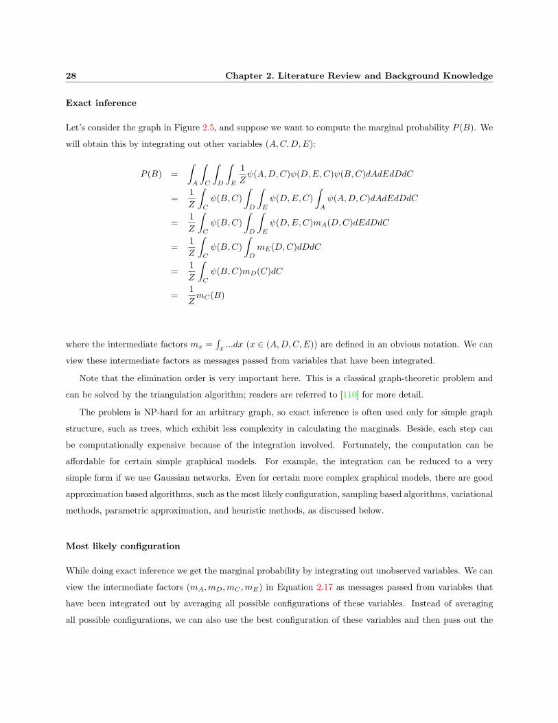
28 Chapter 2. Literature Review and Background Knowledge
Exact inference
Let’s consider the graph in Figure 2.5, and suppose we want to compute the marginal probability P (B). We
will obtain this by integrating out other variables (A,C,D,E):
P (B) =∫
A
∫C
∫D
∫E
1Zψ(A,D,C)ψ(D,E,C)ψ(B,C)dAdEdDdC
=1Z
∫C
ψ(B,C)∫
D
∫E
ψ(D,E,C)∫
A
ψ(A,D,C)dAdEdDdC
=1Z
∫C
ψ(B,C)∫
D
∫E
ψ(D,E,C)mA(D,C)dEdDdC
=1Z
∫C
ψ(B,C)∫
D
mE(D,C)dDdC
=1Z
∫C
ψ(B,C)mD(C)dC
=1ZmC(B)
where the intermediate factors mx =∫
x...dx (x ∈ (A,D,C,E)) are defined in an obvious notation. We can
view these intermediate factors as messages passed from variables that have been integrated.
Note that the elimination order is very important here. This is a classical graph-theoretic problem and
can be solved by the triangulation algorithm; readers are referred to [110] for more detail.
The problem is NP-hard for an arbitrary graph, so exact inference is often used only for simple graph
structure, such as trees, which exhibit less complexity in calculating the marginals. Beside, each step can
be computationally expensive because of the integration involved. Fortunately, the computation can be
affordable for certain simple graphical models. For example, the integration can be reduced to a very
simple form if we use Gaussian networks. Even for certain more complex graphical models, there are good
approximation based algorithms, such as the most likely configuration, sampling based algorithms, variational
methods, parametric approximation, and heuristic methods, as discussed below.
Most likely configuration
While doing exact inference we get the marginal probability by integrating out unobserved variables. We can
view the intermediate factors (mA,mD,mC ,mE) in Equation 2.17 as messages passed from variables that
have been integrated out by averaging all possible configurations of these variables. Instead of averaging
all possible configurations, we can also use the best configuration of these variables and then pass out the

2.3. Bayesian Graphical Models 29
message. This approach is called most likely configuration.
The most likely configuration approach has been widely used. Maximum likelihood estimation (MLE) and
maximum a posteriori (MAP) are special cases of using the most likely configuration approach to estimate
the parameters while learning. The Viterbi algorithm used for Hidden Markov Model decoding is a special
case of using the most likely configuration approach to find the best label of data while testing.
Monte Carlo methods
Given a set of known variables XE , Monte Carlo methods use samples of one or more values of the unobserved
variables XF . In these methods messages passed from a set of nodes are in the form of samples.
Commonly used Monte Carlo methods, such as importance sampling, rejection sampling, the Metropolis
method and Gibbs sampling, can be used to obtain a sample of values, (x1, x2, .., xN ), from the probability
distribution P (x). †† Then, these samples can be used to answer virtually any question φ about the
distribution P(x) by formulating the question in the form:
∫φ(x)P (x)dx ' 1
N
N∑i=1
φ(xi) (2.17)
For example, we can estimate some function of the posterior probability distribution, such as mean, variance,
divergence using Equation 2.17.
Among these Monte Carlo methods, the Metropolis method and Gibbs sampling can be practical in high
dimensional spaces. For more detail of Monte Carlo methods, please refer to [142][143][92].
2.3.5 Bayesian experimental design and sequential decision problem
For most tasks, model estimation is only an intermediate step in the whole process, and the task of a system
is usually to make a decision on which action to take. A good system chooses the best action (such as
delivering or not delivering a document to the user) to maximize some expected utility function, such as the
linear utility function defined in Equation 2.4. A decision is usually made based on the current belief about
the parameters. A comparatively formal description about how to make the decision is:
Let A = ai, i ∈ I be the set of alternative actions available to the system. For each ai, based
on the initial belief about the parameter P (θ) and additional information obtained after
observing data X, we can estimate the possible consequences Cij that may occur after action
††In Bayesian graphical modeling framework P (x) could be the posterior distribution P (XF |XE). Here we use P (x) forrepresentational convenience.

30 Chapter 2. Literature Review and Background Knowledge
ai. Let U(Cij) be the utility corresponding to the consequences if action ai (such as delivering
a document) is taken and we get a consequence Cij (such as the user likes the document).
Then, action a1 is to be preferred over action a2 if and only if:
E(U(a1|X)) > E(U(a2|X)) (2.18)
where
E(U(ai|X)) =∑
j
U(Cij)P (Cij |ai, P (θ), X)
.
So, in order to decide which action to take, one very important part is to specify a utility function that
reflects accurately the purpose of the system.
For example, if the filtering system’s objective is to maximize the immediate T9U utility, system needs to
decide whether to deliver a document or not, and the possible consequences are either the document is relevant
or not, then we have: A = a1, a2, a1 = deliver, a2 = notdeliver, C1,1 = relevant, C1,2 = non− relevant,
C2,1 = relevant, C2,2 = non− relevant, UC1,1 = 2, UC1,2 = −1, and UC2,1 = UC2, 2 = 0.
According to Equation 2.18, the action a1 = deliver is preferred over action a2 =“not deliver” if and
only if:
0 < E(U(a1|X))− E(U(a2|X))
= U(C1,1)P (C1,1,|a1, P (θ), X) + U(C1,2)P (C1,2,|a1, P (θ), X)
+U(C2,1)P (C2,1,|a2, P (θ), X) + U(C2,2)P (C2,2,|a2, P (θ), X)
= 2 ∗ P (relevant|delivered, P (θ), X)− P (non-relevant|delivered, P (θ), X)
= 2 ∗ P (relevant|P (θ), X)− P (non-relevant|P (θ), X)
The last step is based on the assumption that whether to deliver or not to deliver a document does not
affect the relevance of a document. So the system should deliver a document to the user if and only if the
probability of relevance is higher than 1/3 based on current belief about θ.
However, an online system, such as a filtering system, needs to make sequential decisions to optimize a
long term objective function instead of the immediate utility in the previous simple example. To do that,
the system first takes an action based on information learned from the old data, and gets the consequence

2.3. Bayesian Graphical Models 31
together with more information after the action. Then the system revises its belief and chooses another
action, and gets a consequence with further information. The whole online process keeps on until the end
when the final evaluation is made. This is a sequential decision problem where successive interdependent
decisions are to be made. An important area, Bayesian Experimental Design, is devoted to solving such
problems.
A Bayesian decision theory approach to this problem can be summarized as follows [88][34].
Bayesian Experimental Design: An experiment/action a must be chosen from some set A = ai, i ∈ I
after which a data y (∈ Y ) will be observed. The unknown parameter are θ and the parameter space is
Θ. P (y|a) can usually be estimated based on an initial belief about the parameter P (θ) and additional
information X obtained before the action a is taken. There are two decision problems: The selection
of action a and the selection of terminal decision d(∈ D). A general utility function is of the form
U(d, θ, a, y). For any action a, the expected utility of the best decision function is given by
U(a) =∫
y
maxd∈D
∫Θ
U(d, θ, a, y)P (θ|y, a)P (y|a)dθdy (2.19)
The utility function defined here is not necessarily to be the same as defined in Equation 6.1, even if
the global objective function is Equation 6.1. There are many alternative utility functions used by other
researchers for sequential decision problems. Detailed discussion about these various utility functions is
available in [34]. In Section 4.1.2, we will derive a utility function to maximize the global objective function.
In finite states finite horizon sequential decision problem, if the number of possible scenarios (states) at
any given time is finite and if the number of decision nodes to be considered is finite, backward induction can
be used to find the global optimal action [23]. This means that if we know when the user will stop using the
filtering system, theoretically we can find the optimal active learning strategy. Unfortunately, usually this
condition does not hold for the adaptive filtering task. Even if it holds, an exact optimal solution may not be
practical because the computation is usually very expensive. Filtering can be modeled as a continuous multi-
bandits problem [93], a branch of a more general optimal stopping problem. Although the solution described
in [93] probably can’t be applied to the adaptive filtering task because of its computational complexity, it
does provide some useful guidance for us to solve the adaptive filtering task. For example, the exploration
and exploitation we will discuss in Section 4.1.2 can be viewed as one special approximate solution in this
framework.

Chapter 3
Integrating Expert’s Heuristics usingBayesian Priors
As mentioned before, the filtering task shares some common problems, such as document representation and
query representation, with the text classification task and the ad hoc retrieval task. Thus algorithms used for
text classification tasks or the ad hoc retrieval relevant feedback task such as SVMs, logistic regression models,
Naive Bayes, decision trees, language modeling, or Rocchio can be used for profile updating (Section 2.2.2).
Although a large literature about these algorithms exists, there is no conclusion about which algorithm works
best. The purpose of profile learning is to find a classifier with the least generalization error on future data
using the training data available, thus the answer usually depends on the data set. In order to understand
which algorithm works better under what kinds of situations, we can decompose the generalization error of
a learning algorithm into 3 parts:
• Bias: Measure of how closely the learning algorithm is able to approximate the best solution.
• Variance: Measure of how sensitive the learning algorithm is to the training sample.
• Noise: Measure of the inherently irreducible uncertainty of the problem. For example, for a given x
there are more than one possible y.
A high variance means the learning algorithm converges to its asymptotical classifier very slowly. A high bias
means the asymptotical classifier is far from the theoretically optimal classifier. For problems with many
training samples, the bias can be the dominant contributor to the generalization error, while for problems
with very few training samples, the variance may be a dominant contributor. One may want to use a learning
algorithm with both low bias and low variance. However, there is a natural “bias-variance trade-off” for any
learning algorithm [58].
Bias-Variance Dilemma As the complexity of the learning algorithm increases, the bias goes down, but
the variance goes up.
32

3.1. Existing algorithms 33
Because of this dilemma, some complex learning algorithms, such as SVM or logistic regression, may work
well when the amount of training data is large, but some simple algorithms, such as naive Bayesian or
Rocchio, may work better when the amount of training data is very small.
At the early stage of filtering, we have very few training data, thus a low variance learning algorithm
could be a better choice. When we have enough training data later based on long term interaction with the
user, a low bias learning algorithm may work better. However, an adaptive filtering system needs to work
consistently well in the whole filtering process.
We hypothesize that using a Bayesian prior to combine two different algorithms may solve this problem.
In this chapter, we develop a new technique to use the decision boundary of the low variance algorithm as
prior knowledge to set the prior distribution of a low bias model, and then use the data to learn the posterior
distribution of the low bias model. The combined algorithm may get a good bias-variance trade-off based
on the size of the training set, thus achieving a consistent good performance at different stages of filtering.
We apply the proposed technique to combine Rocchio, a heuristic algorithm proposed by an IR expert, with
logistic regression, a widely used statistical machine learning algorithm. An adaptive filtering system using
the new algorithm behaves similar to Rocchio at the early stage of filtering, and becomes more similar to
logistic regression as more user feedback is available. When a user profile contains an initial query, the
proposed algorithm is significantly better than both Rocchio and logistic regression, and compares favorably
with the best methods in the TREC-9 and TREC-11 adaptive filtering tasks. On the TDT5 data set where
no initial query is available, the new algorithm is similar to logistic regression and among the best on TDT
2005 supervised tracking task.
This chapter describes how we develop and evaluate the proposed solution. It is organized as follows:
Section 3.1 introduces the definition of the Rocchio algorithm, logistic regression algorithm. A new algorithm
Logistic Rocchio that combines the Rocchio algorithm and logistic regression is introduced in Section 3.2.
Section 3.3 and Section 3.4 describes our experimental methodology and results. Further discussion and
some related works are provided in Section 3.5. Section 3.6 concludes.
3.1 Existing algorithms
At a certain point in the adaptive filtering process, suppose we have t training documents with user feedback
Dt = (X,Y )t = [(x1, y1), (x2, y2), ..., (xt, yt)], where xi (i = 1 to t) is a vector that represents the document
di in a K dimensional space indexed by K keywords∗. y=1 if the document x is relevant, otherwise y=-1.
∗Any weighting schema, such as TF · IDF , can be used to convert a document di into its vector representation xi.

34 Chapter 3. Integrating Expert’s Heuristics using Bayesian Priors
The core problem in relevance filtering is estimating the posterior probability of relevance of document x
based on the training data: P (y = 1|x, Dt). †
As mentioned before, many algorithms can be used for profile learning. This section introduces two very
representative algorithms: the Rocchio algorithm and logistic regression.
3.1.1 Rocchio algorithm
A widely used profile updating methods in the information retrieval community are different variations of
the incremental Rocchio algorithm [6][29][132][15], which can be generalized as:
Q′= α ·Q + β
∑xi∈R xi
|R|− γ
∑xi∈NR xi
|NR|(3.1)
where Q is the initial profile vector, Q′= (wr1, .., wrK) is the new profile vector, R is the set of relevant doc-
uments, and NR is the set of non-relevant documents. When there is no relevant or non-relevant documents,
the corresponding component in Equation 3.1 is deleted. The Rocchio algorithm also works reasonably under
such kind of conditions.
When a document arrives, the Rocchio algorithm only provides a score indicating how well the document
matches each user profile. ‡ The score is calculated by measuring the distance between the document vector
and the user profileQ′. Since an adaptive system needs to make a binary decision for each incoming document
(e.g., choose from action “deliver” or “not deliver”), researchers usually have to use another module to learn
the dissemination thresholds [155][164]. The filtering system will deliver document x to the user if and only
if its score is above the dissemination threshold. The corresponding decision rule is:
deliver if and only if (wr1, .., wrK)T x >= threshold (3.2)
Let wr0 = −threshold, wTR = (wr0, wr1, .., wrK). If we make x a K+1 dimension vector with the first
dimension corresponding to a pseudo-feature which is always equal to 1, the above equation can be rewritten
†Through out this dissertation, we use a symbol in bold font to represent a vector.‡The same is true for many other statistical retrieval algorithms that were originally designed for ad hoc retrieval, where a
ranking of documents is sufficient.

3.1. Existing algorithms 35
as: §
deliver iff wTRx >= 0 (3.3)
The Rocchio algorithm is popular for two reasons. First, it is computationally efficient for online learning
[6]. Second, compared to many other algorithms, it works well empirically [15][164]. However, the Rocchio
algorithm is not based on a strong probabilistic framework and there is no guarantee about whether it will
provide the optimal decision boundary in the high dimensional document space asymptotically, with infinite
training data. In other words, the Rocchio algorithm is a simple heuristic algorithm that works empirically
well.
3.1.2 Logistic regression
Logistic regression is one widely used statistical algorithm that can provide an estimation of the posterior
probability P (y|x) of an unobserved variable y given an observed variable x. It has been widely used in the
statistical and machine learning community.
A logistic regression model estimates the posterior probability of y via a log linear function of observed
document x.
P (y = ±1|x,w) = σ(ywT x) =1
1 + exp(−ywT x)
where w is the K dimensional logistic regression model parameter learned from the training data.
Before filtering, the Bayesian based learning system usually begins with a certain prior belief p(w) about
the distribution of the logistic regression parameter w (Section 2.3.1).
A Gaussian distribution p(w) = N(w;mw, vw) is often used as the prior distribution for logistic regression
weights, where mw is the mean of the Gaussian distribution in the K dimensional parameter space and v−1w
is a (K + 1) · (K + 1) covariance matrix of the Gaussian distribution.
If there is no obvious correlation between the different dimensions of w, or if we can’t tell what the
correlations are, the off-diagonal values in the matrix v−1w are usually set to zero. If we are not very
confident about whether the true value of w is mw, the diagonal variables of the matrix v−1w are usually
set to a small number. If all items in matrix v−1w are zero, p(w) is a non-informative prior: all values of w
have the same probability. A non-informative prior may seem objective as it represents the idea of letting
the data speak for themselves. However, a classifier learned using a non-informative prior usually over fits
§For convenience, depending on the context, we use x to represent K dimensional vector or K+1 dimensional vector in thedissertation.

36 Chapter 3. Integrating Expert’s Heuristics using Bayesian Priors
the data. So, v−1w is usually set to a diagonal matrix with a small non-zero positive number on the diagonal
to act as a regularizer. The effect is the same as smoothing techniques used while building language models
[162]. [162] presents smoothing with priors for generative models, while we are regularizing with priors for
discriminative models.
At a certain point in the adaptive filtering process, we can update our belief about the logistic regression
parameter w conditional on the training data Dt using Bayesian theorem.
P (w|Dt) =P (Dt|w)P (w)∫wP (Dt|w)P (w)
=∏t
i=1 P (yi|w,xi)P (w)∫w
∏ti=1 P (yi|w,xi)P (w)
With a Gaussian prior N(w;mw, vw)), the maximum a posteriori MAP estimation of w is:
wMAPt= argmaxwP (w|Dt)
= argmaxw
t∏i=1
P (yi|w,xi)P (w)
= argmaxw
t∑i=1
log(1 + exp(−yiwT xi))− vw(w −mw)2
Equation 3.4 can be viewed as a special form of regularized logistic regression, where vw controls the
strength of the regularizer. There is no closed form solution for wMAPt , so greedy search algorithms, such
as conjugate gradient descent, are often used to find the wMAPt . In most of the cases where we have no
prior knowledge about what the logistic regression parameter is, we usually set w = (0, ..., 0) and v−1w to a
very small value. Then, we get a norm-2 regularized logistic regression model:
wMAPt= argmaxw
t∑i
log(1 + exp(−yiwT xi))− vww2 (3.4)
When a new document x arrives, we can estimate the probability of relevance for this document:
P (y = 1|x) = P (y = 1|x,wMAPt) (3.5)

3.2. New algorithm: LR Rocchio 37
3.2 New algorithm: LR Rocchio
At the early stage of filtering when the system has very few training data, a simple profile learning algorithm
with low variance, such as the Rocchio algorithm with a good thresholding method, is likely to be a good
choice. At the later stage of filtering when the system has enough training data, a complex profile learning
algorithm with low bias, such as logistic regression, may be better. How do we get an algorithm that works
well consistently over the whole filtering process? One possible approach is to use the Rocchio algorithm
first, then switch to logistic regression later when the amount of training data is enough. Another approach
is to combine the Rocchio algorithm and logistic regression together to get a natural and smooth trade-off
between variance and bias. The second approach, which will be explored further in this section, is the
motivation for the new algorithm, a combination of Rocchio and logistic regression based on a Bayesian
prior.
As mentioned before, Bayesian priors are a widely used tool for introducing human knowledge into model
building; and it is also a regularizing tool for controlling the model complexity and avoiding overfitting. An
adaptive filtering task begins with a very small amount of training data, thus a stable prior that works well
with little training data is very important for building a good filtering system. Since the Rocchio algorithm
is designed by researchers in IR community and works well empirically in the adaptive filtering task, using it
to set a Bayesian prior of the logistic regression model parameter may help us to achieve stable performance
at the early stage of filtering.
Usually, a logistic regression prior is a Gaussian distribution N(mw, vw). How does one find the prior
mean mw from Rocchio? A new technique is proposed here to solve this problem.
Let wR = (wr0, wr1, wr2, wr3..., wrK) be the profile vector calculated based on the Rocchio algorithm
(Equation 3.3).
For logistic regression, we use the same representation as Rocchio for documents: the same set of keywords
with the same weighting schema, plus a pseudo-dimension, which is always 1, as features. The probability
of relevance of a given document x based on logistic regression model w is:
P (y = 1|x,w) =1
1 + exp(−wT x)
If the goal is to minimize classification error, a filtering system using the logistic regression model will:
deliver if and only if wT x >= 0 (3.6)

38 Chapter 3. Integrating Expert’s Heuristics using Bayesian Priors
Equation 3.3 and Equation 3.6 are very similar. If the threshold of a Rocchio learner is set to minimize
classification error too, both algorithms are trying to find a linear decision boundary in the high dimensional
space indexed by the set of keywords for the same objective. A Gaussian prior N(w;mw, vw) for logistic
regression encodes the belief that the true decision boundary is around the one defined by mw. Instead of
setting mw = (0, ..., 0), if we set mw so that the decision boundary of it is the same as the one found by
Rocchio, N(w;mw, vw) may be better than the commonly used non-informative prior or zero mean Gaussian
prior.
A prior mw that encodes Rocchio’s suggestion about decision boundary can be learned via constrained
maximum likelihood estimation:
mw = argmaxw
t∑i=1
log(1
1 + exp(−yiwTxi)) (3.7)
under the constraint: cos(w,wR) = 0 (3.8)
The resulting logistic regression parameter mw maximizes the likelihood of the data (Equation 3.7) under
the constraint that it corresponds to the same decision boundary as the Rocchio algorithm (Equation 3.8).
This is an optimization problem, and the solution is in a simple form that can be calculated efficiently:
mw = α∗ ·wR (3.9)
where α is a scalar:
α∗ = argmaxα
t∑i=1
11 + exp(−yiαwT
Rxi)
This is a one dimensional optimization problem, and the solution can be found quickly using gradient descent
algorithms.
The Rocchio algorithm tends to be more stable at the early stage of filtering, especially given an initial
query. The decision boundary found by Rocchio is likely to be better than the one found by logistic regression.
As an extreme example, if the system has only an initial query without training data, Rocchio can still provide
reasonable performance, while we can’t learn a logistic regression model. At the early stage of filtering when
the amount of training data is small, the prior is very important, thus the influence of the Rocchio algorithm
on the logistic regression model is strong. When the system gets more and more training data, the prior is less
important, and logistic regression dominates. This technique automatically manages the trade-off between
bias and variance based on the amount of training data available. With the Bayesian prior estimated using
Rocchio, the logistic regression parameter estimated has a higher bias but lower variance than without a

3.3. Experimental methodology 39
prior. As more and more training data are available, the bias decreases. Asymptotically, the learned classifier
converges to the optimal linear decision boundary in the high dimensional document space.
3.3 Experimental methodology
Some experiments are carried out to understand the proposed new algorithm and compare it with the
Rocchio algorithm (Equation 3.1), Norm 2 regularized logistic regression algorithm 3.4, logistic regression
with unscaled Rocchio weights wr as the prior mean, and the best methods in TREC-9 and TREC-11
adaptive filtering tasks. We set the variance of the prior according to our confidence about the prior
distribution. For example, we feel more confident about the prior mean set by the scaled Rocchio weight
α∗wR, thus we set the variance of the prior mean to a comparatively smaller number, 10I, where I is an
identity matrix (also known as unit matrix). While using other prior means, such as zero used in the Norm
2 regularized logistic regression model, we are less confident about whether they are close to the optimal or
not, thus we set the variance of the prior mean to a larger number, 100I. The Rocchio weights (α, γ, λ) is
set to (1, 3.5, 2) as [164].
The experiments follow the requirements specified by TREC adaptive filtering tasks [119][121]. The whole
task models the text filtering process from the moment user arrives with a small amount of identified relevant
documents and a natural language description of the information need. Documents arrive before user profile
construction, among which only 2 or 3 are labeled, can be used as training data to learn word occurrence
(e.g., idf) statistics, corpus statistics (e.g., average document length), and the initial profile representation.
Remaining documents in the incoming documents stream are testing data. As soon as a new document
arrives, the system makes a binary decision about whether or not deliver it to the user. If it is delivered,
the relevance judgment for that document is released to the system and added to the training data set for
profile updating.
The system treats the initial user profile description, which includes the title and description fields of
the corresponding topic provided by NIST, as a relevant document while training logistic regression models.
As a TREC adaptive filtering run begins with no non-relevant documents, our system randomly samples a
small number (<= 3) documents and uses them as non-relevant documents to train logistic regression and
Logistic Rocchio models. Documents are represented as vectors using a variation of INQUERY’s TF · IDF
weighting [6]. ¶
¶We set xi,d = tfbeli,d · idfi, where tfbeli,d =tfi,d
tfi,d+0.5+1.5lend
avgDocLen
, idfi = log(N+0.5dfi
/ log(N + 1)), tfi,d is the number of
times term i occurs in document d, lend is the length of document d, avgDocLen is the average length of documents processed,N is the number of documents processed, and dfi is the number of documents that contain term i.

40 Chapter 3. Integrating Expert’s Heuristics using Bayesian Priors
Table 3.1: A comparison of different algorithms on the TREC-9 OHSUMED data set.Rocchio LR1 LR2 LR Rocchio
Prior Mean NA 0 wR α∗wR
T11SU 0.37 0.36 0.12 0.39T9U 11.38 10.43 -24.54 15.03
Precision 0.37 0.30 0.10 0.37Recall 0.19 0.21 0.20 0.23
Doc/Profile 20.10 24.67 62.87 23.78
Three different text corpora are used to evaluated the proposed algorithms in our experiments: the
OHSUMED data set used in the TREC-9 Filtering Track (Section 2.1.2), the Reuter’s 2001 data set used in
the TREC-11 Filtering Track (Section 2.1.2), and the multi lingual data set used in the TDT5 supervised
tracking task (Section 2.1.2).
3.4 Experimental results
The experimental results on the OHSUMED data set are in Table 3.1. The Rocchio algorithm has reasonable
performance, among the best compared to other filtering systems that participated in the TREC-9 adaptive
filtering task [119]. ‖ Logistic regression with a prior N(w; 0, 100I) (LR1) is a little worse, but still good.
Logistic regression using the prior N(w;wR, 10I) (LR2) is bad. This indicates using wR directly estimated
by the Rocchio algorithm as the prior mean is very misleading. However, after scaling using Equation 3.9
and setting the prior to N(w;α∗wR, 10I) (LR Rocchio), we get a significant improvement. This confirms
our hypothesis that combining Rocchio with logistic regression will work well. This is not surprising since
using a low variance classifier to set the prior for a low bias classifier may provide a nice trade-off between
variance and bias.
The experimental results on Reuter’s data set are in Table 3.2 and Table 3.3. ∗∗ The Rocchio algorithm
gets reasonable performance. Logistic regression with the prior with zero mean is a little better. Logistic
regression using the Gaussian prior with wR as the mean performs poorly. Using the scaled Rocchio weight
(Equation 3.9) as the prior performs the best.
Figures 3.1 and Figure 3.2 compare the performance of the new algorithm with the Rocchio and logistic
regression algorithms on each individual profile using T11U measure to get an idea of how significant the
improvement is on a query by query basis. We can see that for most of the profiles, the new algorithm works
‖The T9U values of the top 3 TREC participants on this data set are: 17.3, 10.7 and 10.1.∗∗The final relevance judgments used in Table 3.2 are a little better than the old relevance judgments used in Table 3.3
(Section 2.1.2.).

3.4. Experimental results 41
Table 3.2: A comparison of different algorithms on the TREC-11 Reuter’s data set.Rocchio LR1 LR2 LR Rocchio
Prior Mean NA 0 wR α∗wR
T11SU 0.46 0.49 0.16 0.52T11U 63.06 76.60 -25.86 83.10
Precision 0.53 0.48 0.20 0.56Recall 0.33 0.41 0.46 0.41
Doc/Profile 69.36 88.28 223.32 84.12
Table 3.3: A comparison of different algorithms on the TREC-11 Reuter’s data set using the old relevancejudgments.
Rocchio LR1 LR2 LR RocchioPrior Mean NA 0 wR α∗wR
T11SU 0.46 0.49 0.11 0.54T11U 40.20 54.66 -32.38 61.68
Precision 0.51 0.46 0.18 0.54Recall 0.35 0.49 0.50 0.50
Doc/Profile 47.22 69.96 165.04 66.18
better (above the horizontal line). A statistical test (sign test) indicates that the new algorithm is significant
better than the Rocchio algorithm and logistic algorithm.
Figure 3.3 compares the performance of our system with other systems that participated in the TREC11
adaptive filtering task. In TREC11, each participant submitted 1-4 runs to NIST, and the best run of each
individual participant is reported here. A system that delivers nothing will get T11SU=0.33, and some
TREC-11 participating systems are lower than that. The logistic regression and the Rocchio algorithm are
among the best of TREC participants, while the proposed algorithm (Logistic Rocchio) is much better than
the best runs submitted by the TREC-11 adaptive filtering task participants. In Section 2.3.1, we mentioned
that a prior helps us to control model complexity as well as introduce prior knowledge into model building.
Both LR Rocchio and logistic regression models benefit from the use of prior to control model complexity,
thus work well. LR Rocchio also benefits from the prior knowledge/heuristics, thus works the best.
We also compare the accumulated performance of different profile learning algorithms over time on the
TREC-11 adaptive filtering task (Figure 3.4). Rocchio works better than logistic regression at the early stage
of filtering, but worse at later stages. Logistic regression with a Rocchio prior is the best at any time. This
is not surprising based on the bias-variance analysis. The new algorithm Logistic Rocchio, is consistently
much better than the other two.
To study the effectiveness of the proposed algorithm filtering solution to a similar but different task where

42 Chapter 3. Integrating Expert’s Heuristics using Bayesian Priors
0 10 20 30 40 50
−4
0−
20
02
04
06
0
Difference of Utility between logistic regression Rocchio with logistic regression
topics
Utilit
yL
RR
− U
tilit
yL
R
Figure 3.1: Comparison of the performance on individual pro-file: T11U of Logistic Rocchio - T11U of LogisticRegression.
0 10 20 30 40 50
−5
00
50
10
01
50
20
02
50
Difference of Utility between logistic regression Rocchio with Rocchio
topics
Utilit
yL
RR
− U
tilit
yR
occh
io
Figure 3.2: Comparison of the performance on individual pro-file: T11U of Logistic Rocchio - T11U of Rocchio.

3.4. Experimental results 43
Figure 3.3: Comparison with other TREC participants. The T11SU values of different runs on the TREC-11adaptive filtering task are reported in this figure. Systems in the legend from top to bottom correspond tobars from left to right. Our results and the results of TREC-11 participants are not directly comparable,because we have had greater experience with the dataset. The figure is provided only to give context for theresults reported in this dissertation.

44 Chapter 3. Integrating Expert’s Heuristics using Bayesian Priors
3 4 5 6 7 8 9
x 105
0.4
0.42
0.44
0.46
0.48
0.5
0.52
Documents Passed
T11S
U
T11SU over time on TREC11 Filtering Track Data
Logistic Regression + Rocchio PriorLogistic RegressionRocchio
Figure 3.4: A comparison of the performance of different profile learning algorithms over time on the TREC-11 adaptive filtering task. This figure is the average of 50 user profiles.
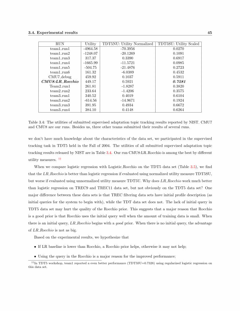
3.4. Experimental results 45
RUN Utility TDT5NU: Utility Normalized TDT5SU: Utility Scaledteam1 run1 -4964.58 -70.3956 0.0270team1 run2 -1248.07 -20.1269 0.1091team1 run3 317.37 0.3390 0.6917team1 run4 -1665.99 -11.5721 0.0985team1 run5 -504.75 -21.4876 0.2723team1 run6 161.32 -6.0389 0.4532
CMU7 debug 459.92 0.1037 0.5911CMU8:LR Rocchio 449.17 0.5921 0.7281
Team2 run1 261.81 -1.8287 0.3820team2 run2 233.64 -1.4206 0.3575team3 run1 340.52 0.4019 0.6104team3 run2 -614.56 -14.9671 0.1924team3 run3 391.95 0.4934 0.6672team3 run4 384.10 0.4148 0.6264
Table 3.4: The utilities of submitted supervised adaptation topic tracking results reported by NIST. CMU7and CMU8 are our runs. Besides us, three other teams submitted their results of several runs.
we don’t have much knowledge about the characteristics of the data set, we participated in the supervised
tracking task in TDT5 held in the Fall of 2004. The utilities of all submitted supervised adaptation topic
tracking results released by NIST are in Table 3.4. Our run CMU8:LR Rocchio is among the best by different
utility measures. ††
When we compare logistic regression with Logistic Rocchio on the TDT5 data set (Table 3.5), we find
that the LR Rocchio is better than logistic regression if evaluated using normalized utility measure TDT5SU,
but worse if evaluated using unnormalized utility measure TDT5U. Why does LR Rocchio work much better
than logistic regression on TREC9 and TREC11 data set, but not obviously on the TDT5 data set? One
major difference between these data sets is that TREC filtering data sets have initial profile description (as
initial queries for the system to begin with), while the TDT data set does not. The lack of initial query in
TDT5 data set may hurt the quality of the Rocchio prior. This suggests that a major reason that Rocchio
is a good prior is that Rocchio uses the initial query well when the amount of training data is small. When
there is an initial query, LR Rocchio begins with a good prior. When there is no initial query, the advantage
of LR Rocchio is not as big.
Based on the experimental results, we hypothesize that
• If LR baseline is lower than Rocchio, a Rocchio prior helps, otherwise it may not help;
• Using the query in the Rocchio is a major reason for the improved performance;††In TDT5 workshop, team1 reported a even better performance (TDT5SU=0.7328) using regularized logistic regression on
this data set.

46 Chapter 3. Integrating Expert’s Heuristics using Bayesian Priors
Table 3.5: A comparison of logistic regression (LR) with Logistic Rocchio on the TDT5 Multilingual dataset.
LR1 LR RocchioPrior Mean 0 α∗wR
TDT5SU 0.687 0.72TDT5U 435 399Precision 0.19 0.32Recall 0.92 0.77
Doc/Profile 162.3 99.7
• Using the query in other ways may also help. However, one needs to be careful about how to use the
query, since using it as one training example as in logistic regression (LR1) or using it in as in unscaled
Rocchio prior (LR2) have not help as much as in LR Rocchio.
It’s worth mentioning that the Rocchio algorithm itself is rather heuristic. Different implementations of the
algorithm may perform differently. Because the Rocchio algorithm does not provide the guidance on other
components, such how to set dissemination threshold or how to set term weights and do feature selection,
while these compenents also influence the final result. In TREC adaptive filtering track, Rocchio is used for
profile learning by some of the top ranking systems, as well as some lower ranking systems [119]. Similarly,
the logistic regression algorithm may perform differently. So one may want to test whether the assumptions
hold before using LR Rocchio.
3.5 Related work and further discussion
Although our detailed analysis is focused on combining Rocchio and logistic regression, the proposed tech-
nique can also be applied to combining other learning algorithms. One may ask, how can we tell which
algorithms we should combine? In other words, how can we tell which algorithm has a lower bias, and which
algorithm has a lower variance?
We do not have a good answer to this question. The Bias-Variance Dilemma tells us that the complexity of
the learning algorithm grows, the bias goes down, while the variance goes up. Unfortunately the complexity
of classification algorithms are difficulty to measure, thus it is hard to use this dilemma empirically. In
order to get a better answer to this question, we can compare the following two more general probabilistic
approaches.
Discriminant approach: The posterior distribution P (y|x) is modeled directly. For example, SVM [70]

3.5. Related work and further discussion 47
and logistic regression are popular discriminative models. In this approach, systems directly model the
boundary between classes.
Generative approach: The distributions P (x|y) and P (y) are modeled, and the posterior distribution
P (y|x) is derived using the Bayes rule:
P (y = 1|x) =P (y = 1,x)
P (x)=P (y = 1,x)∑
y P (x|y)
For example, language models [83], Naive Bayes [98], and BIM [122] are popular generative models
used in IR. In this approach, systems first model the characteristics of each classes, and then derive the
boundary between classes. The non-probabilistic Rocchio algorithm has some generative model flavor
in the sense that the centroid of relevant and non-relevant documents are estimated [69, 125].
Some early work suggests that the generative models may have a low variance and work well with
few training data, and comparable discriminative models may have a low bias and work better when the
amount of training data is large [109][126]. Although there is no strong theoretical justification on which
discriminative-generative pairs are low bias/low variance pairs, and the answer may also depend on the
empirical task, combining comparable generative-discriminative models using the technique proposed in this
chapter is likely to give a good performance in adaptive filtering system.
Besides statistical models, systems sometimes also use heuristic approaches or domain knowledge to make
decisions. If we view the Rocchio classifier’s decision boundary or the initial query from the user as domain
knowledge, the proposed solution is a mechanism to integrate the domain knowledge into learning algorithms.
Other domain knowledge can also be integrated into a machine learning algorithm in a similar way by first
converting the domain knowledge into a decision boundary, then converting the decision boundary into a
prior distribution of the model parameters. If the decision boundary derived from the domain knowledge
works well, the final classifier will work well with little training data.
The technique proposed in this chapter has the flavor of a Bayesian analysis. However it is not a strict
Bayesian approach, because the prior is estimated using the data. This is similar to Empirical Bayes methods
[95].
There has been much research on combining different text classification algorithms or retrieval algorithms
in the IR community [80][156][66][18][82]. [80] picks up different classifiers for different categories using
categorical features; [66] [156] and [18] combine the output or transformation of the output of different

48 Chapter 3. Integrating Expert’s Heuristics using Bayesian Priors
classifiers using linear combinations; [21] combines out put of classifiers with probabilistic learning based on
some reliability indicators.
In contrast to the previous research on text classification or retrieval task, our work is different in three
aspects:
• The focus of our work is adaptive filtering task, where the amount of training data changes over time.
• The previous work combines the output of various text classifiers, while the proposed techniques
combines the classifiers based on better understanding of the variance, bias properties of the classifiers
to be combined.
• By using a low variance classifier to set the prior for a low bias classifier, the proposed technique
automatically gets a nice trade-off between variance and bias based on the size of the training data
set. The combined classifier has a low variance when the amount of training data is small, and has a
low bias when the amount of training data is large.
We also noticed a recent independent work that combines generative/discriminative models [115] and they
found the hybrid model is significantly better than either the generative model or the discriminative coun-
terparts. However, they focused on text classification instead of the adaptive filtering task. The combination
technique and the effects of their algorithm are very different from ours. For example, their classifier does
not converge to logistic regression’s optimal estimation when the amount of training data goes to infinity.
Besides the Bayesian’s way of using domain expert’s knowledge or heuristics as a prior distribution of
the parameters to be learned, there are alternative approaches to encode the prior. We can introduce the
prior as constraints for learning a classifier under the maximum entropy or minimum divergence framework.
For example, we can use a regularized logistic regression, with regularizer derived from initial user query,
to achieve similar effect. This alternative approach can be explained under the Bayesian framework as in
Equation 3.4, and different regularizer usually can be converted to different prior distribution.
3.6 Summary
An empirical filtering system needs to works well consistently at all stages of filtering process. Motivated by
Bayes’ theorem, we have developed a new technique to combine two classifiers, using a constrained maximum
likelihood approach to learn a Bayesian prior for one classifier from another classifier. If the classifier used
to learn the prior should have less variance, and if the classifier that uses the prior should have less bias,
the proposed approach provides a reasonable trade-off between variance and bias based on the amount of
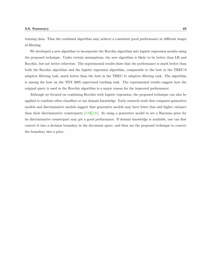
3.6. Summary 49
training data. Thus the combined algorithm may achieve a consistent good performance at different stages
of filtering.
We developed a new algorithm to incorporate the Rocchio algorithm into logistic regression models using
the proposed technique. Under certain assumptions, the new algorithm is likely to be better than LR and
Rocchio, but not better otherwise. The experimental results show that the performance is much better than
both the Rocchio algorithm and the logistic regression algorithm, comparable to the best in the TREC-9
adaptive filtering task, much better than the best in the TREC-11 adaptive filtering task. The algorithm
is among the best on the TDT 2005 supervised tracking task. The experimental results suggest how the
original query is used in the Rocchio algorithm is a major reason for the improved performance.
Although we focused on combining Rocchio with logistic regression, the proposed technique can also be
applied to combine other classifiers or use domain knowledge. Early research work that compares generative
models and discriminative models suggest that generative models may have lower bias and higher variance
than their discriminative counterparts [109][126]. So using a generative model to set a Bayesian prior for
its discriminative counterpart may get a good performance. If domain knowledge is available, one can first
convert it into a decision boundary in the document space, and then use the proposed technique to convert
the boundary into a prior.

Chapter 4
Exploration and Exploitation Trade-off usingBayesian Active Learning
As a system filters, it also refines its knowledge about the user’s information need based on relevance feedback
from the user. Delivering a document has two effects: 1) it satisfies the user’s information need immediately,
and 2) it helps the system better satisfy the user in the future by learning from the relevance feedback about
this document provided by the user. Traditional approaches for adaptive information filtering, including the
filtering experiments we did in the previous chapter, fail to recognize and model this second effect.
The goal of a filtering system is to maximize the utility in the long run. In order to do that, traditional
approaches deliver a document if and only if the expected immediate utility of delivering it is greater
than the expected utility of not delivering it. The expected immediate utility can be calculated from the
probability that the document is relevant. For example, for the utility function used by the TREC-9, TREC-
10 and TREC-11 Filtering Tracks (Equation 2.4), TREC participants usually set the threshold at t where
P (relevant|document score = t) = 1/3 because the expected utility at that point is 0 [12, 164, 118]. In
fact, delivering a document if and only if P (relevant|document score) ≥ 1/3 was written explicitly in the
guidelines of some TREC adaptive filtering tasks [119].
The work in the previous section is also an example of the traditional method that only focuses on
the immediate utility. The system first estimates the uncertainty of the relevant node in Figure 2.1: the
probability of relevance of a document. Then the system estimates the utility (credit or penalty) it can get
immediately after delivering this document. Existing filtering approaches, including what we have done in
previous chapter, do not consider the possibility that the system can improve its knowledge about the user’s
information need based on the feedback from the user so that it can better serve the user in the future.
Especially in the early stage of filtering, when the system’s knowledge about the user’s information need is
very limited, the potential gain from improving the user model can be substantial.
In this section, we go further to study the second aspect and model the long term benefit of delivering a
document. The Bayesian graphical modeling approach provides a principled way to do that because of the
explicit modeling of uncertainty. In Figure 2.1, uncertainty is not only related to the “relevant” node, but
50

4.1. Algorithm 51
also associated with other nodes, such as the “parameter θ” node. So we can also estimate the uncertainty
of the “θ” node: the probability distribution of the model parameter. The notion of uncertainty of θ enables
us to measure the improvement of the user profiles after learning from the user feedback on the delivered
documents.
Maximizing the accumulated utility over a period of time is the objective of a filtering system. To
achieve this goal, we derived a new model quality measure, utility divergence (Section 4.1.2), to help the
filtering measure the quality of a user profile. Unlike measures of model quality used in most active learning
methods, utility divergence has the advantage of having the same scale as the traditional utility model
adaptive filtering systems try to optimize. Thus we can combine the expected immediate utility with the
expected improvement on model quality to get a single quantity that measures the short-term and long-term
value of a document in the document stream. This combined measure is the basis for deciding whether to
deliver the document.
The following subsections describe our research on exploration and exploitation while filtering based on
uncertainty of the model parameters. Section 4.1 describes the general theoretical framework of optimizing
the utility based on the trade-off between exploration and exploitation using Bayesian theory. Sections 4.2
and Section 4.3 describe our experimental methodology and results. Section 4.4 discusses related work and
Section 4.5 concludes this chapter.
4.1 Algorithm
In order to maximize the overall utility of a system, we propose to have two modules for the system: The
exploitation module and the exploration module. The exploitation module estimates the immediate utility of
delivering a new document based on the model parameter learned, while the exploration module estimates
the future utility of delivering a new document by considering the improvement of the model parameter
estimation if we get the user feedback about the document. To trade off exploitation and exploration, the
filtering system delivers a document if the combined utility is above zero.
For simplicity, we use Bayesian logistic regression as our learner. We assume the form of the utility
function to maximize is:
Utility = AR ·R+ +AN ·N+ (4.1)

52 Chapter 4. Exploration and Exploitation Trade-off using Bayesian Active Learning
dtq~P(q|Dt-1)
Relevant
Step 1:
Step 2:
Figure 4.1: Exploitation and exploration for relevance filtering. Step 1: Messages are passed from knownnodes “θ” and “dt” to “relevant” to estimate the probabilistic distribution of “relevant”. Then we canestimate the immediate utility. Step 2: Messages are passed from known nodes “dt” and “relevant” tounknown node “θ” to estimate the probabilistic distribution of “θ”, assuming we know the relevance feedbackabout document “dt”. Then we estimate the future utility gain if dt is delivered, based on the probabilisticdistribution of parameter “θ”.

4.1. Algorithm 53
4.1.1 Exploitation using Bayesian inference
As mentioned before, the direct utility gain/loss due to delivering a document can be calculated once we
know the probability of relevance of that document. Estimating the probability of relevance of a document
based on the model parameter learned corresponds to the first step in Figure 4.1.
In Chapter 3, when a new document arrives, we use the maximum a posteriori MAP estimation of the
model parameter θMAP to estimate the probability of relevance. We can also use the exact inference algorithm
as described in Section 2.3.4. Suppose we have a model parameterized as θ to estimate the probability of
the relevance of a given document. The prior distribution of the model parameters is p(θ). After seeing data
D = {(x1, y1), · · · , (xk, yk)}, the posterior distribution p(θ|D) is:
p(θ|D) =P (D|θ)p(θ)∫P (D|θ)p(θ)dθ
(4.2)
where P (D|θ) is the likelihood of the user feedback given delivered documents and θ.
P (D|θ) =∏
i
P (yi|xi, θ) (4.3)
The exact Bayesian average of the immediate utility gain of delivering a document is:
U1(x|D) =∫
θ
∑y
AyP (y|x, θ)P (θ|D)dθ (4.4)
where Ay is the utility of delivering a document x if the true label of x is y. According to Table 2.1, Ay = AR
if the true label is “relevant”, and Ay = AN if the true label is “non-relevant”.
4.1.2 Exploration using Bayesian active learning
For exploration, we need to measure the improvement on the learned model if we deliver the document. This
corresponds to the second step in Figure 4.1. ∗
In order to quantify the improvement, a measure of the quality of the learned model is needed. It will
enable us to estimate the improvement of a model once we know the label of a document compared to the
model learned before delivering the document. The goal of estimating a model is to help the system make
future decisions, and the object of the system is the utility function. Thus a reasonable measure for the
model quality should be based on the utility function.∗We assume the “relevant” node is known in Step 2 because we have an estimate of the distribution of this node as a result
of step 1.

54 Chapter 4. Exploration and Exploitation Trade-off using Bayesian Active Learning
In the active learning framework proposed by [145], if we choose to use model θ and the true model is θ,
we incur some loss Loss(θ||θ). Although we do not know the exact value of θ, p(θ|D) represents our beliefs
about the distribution of θ given the evidence. Thus the expected loss of using model θ is given by:
Loss(D, θ) = ED(Loss(θ, θ))
=∫
θ
p(θ|D)Loss(θ||θ)dθ (4.5)
where p(θ|D) is the posterior distribution of different model parameters. The quality of a model after we
have seen data set D is:
Loss(D) = Loss(D, θ∗D) (4.6)
where θ∗D = argminθ Loss(D, θ) if the system makes decisions using the model that minimizes the lose. †
Smaller Loss(D) means a better model. For active learning, Loss(θ, θ∗D) needs to capture the notion
of uncertainty of the model parameters. One commonly chosen metric is Kullback-Leibler divergence (KL-
divergence) [145]:
KL(θ||θ∗D) =∫p(x)
∑y
p(y|x, θ) logP (y|x, θ)P (y|x, θ∗D)
dx
where p(x) is the distribution of input x, which is independent of θ and is usually given or learned from
unlabeled data.
The usefulness of knowing the label of a document is measured by its potential to lower Loss(D). However,
in information filtering the ultimate goal is to optimize some utility function in the long run. It is unclear
how a smaller KL-divergence relates to higher utility. It is also unnatural to combine KL-divergence with the
expected immediate utility credit/loss to get a single quantity on which the decision of whether to deliver
a document can be made. So, instead of using KL-divergence, we propose to use the difference between
the best possible utility and the actual utility, which we call utility divergence, as the function Loss(θ, θ) to
measure the model quality:
UD(θ||θ) = U(θ, θ)− U(θ, θ) (4.7)
where U(θ′, θ′′) is the expected utility if we choose to use model θ′′ and the true model is θ′. A well-defined
U(θ′, θ′′) should have the following property
∀θ′, θ′′, U(θ′, θ′) ≥ U(θ′, θ′′) (4.8)†If the system makes decisions differently, we need to change it accordingly.

4.1. Algorithm 55
which essentially says that the expected utility of an incorrect model cannot exceed the expected utility
of the correct model. It is worth noting that KL-divergence proposed by [144] is a special case of utility
divergence. If we choose to use log-likelihood as utility, then U(θ′, θ′′) is:
U(θ′, θ′′) =∫p(x)
∑y
p(y|x, θ′) logP (y|x, θ′′)dx
which shows that when using log-likelihood as utility, UD(θ||θ) = KL(θ||θ).
Using utility divergence as the loss function, Loss(D) can be rewritten as shown below.
Loss(D)= Loss(D, θ∗D)
=∫p(θ|D)(U(θ, θ)− U(θ, θ∗D))dθ (4.9)
For information filtering, the goal is to maximize the utility (Equation 4.1), so we define:
U(θ′, θ′′) =∫
S(θ′′)
p(x)∑
AyP (y|x, θ′)dx (4.10)
where S(θ′′) = {x|∑
y AyP (y|x, θ′′) > 0} is the space of x where model θ′′ “thinks” delivering x has
immediate positive utility.
The expected reduction of utility divergence due to knowing the label of a document x for the next
immediate future (the document right after the current one) is:
U2(x|D) =∑
y
P (y|x,D)Loss(D ∪ (x, y))− Loss(D) (4.11)
If there are Nfuture (discounted) future documents, then the expected utility of delivering document x is: ‡:
U(x|D) = U1(x|D) +NfutureU2(x|D) (4.12)
We deliver a document x if and only if U(x|D) ≥ 0.
The whole process from a Bayesian graphical modeling point of view is summarized in Figure 4.1. The
system first treats node “relevant” as unknown, and estimates its distribution based on the known nodes
“document” and “θ”. This estimation is used to calculate the immediate utility gain of delivering the
document (Equation 4.4. Then, the system treats the nodes “relevant” and “document” as known, and‡This assumes that the system does not change its model while filtering the following Nfuture documents, and the assumption
makes the computation less complex.

56 Chapter 4. Exploration and Exploitation Trade-off using Bayesian Active Learning
estimates the probability distribution of the parameter node “θ”. The Utility Divergence derived based on
the probability distribution of value of the parameter node is then used to measure the quality of the new
model if we know the label of “relevant” node. The quality of the new model minus the quality of the old
model is the expected reduction of the expected loss of utility, and this is used as the measure of the future
utility gain of delivering the document. When it is combined with the immediate utility, we get a complete
estimation of the utility gain (Equation 4.12).
4.1.3 Determining the dissemination threshold based on logistic regression
The proposed algorithm can be applied to a high dimensional space for learning term weights with statistical
based profile learning methods, such as the LR Rocchio algorithm we proposed before. However, the com-
putational complexity of using the proposed algorithm with LR Rocchio can be very expensive, considering
the integration in Equation 4.4 and 4.11. It may takes months to process the standard evaluation data, such
as 4 years of US National Library of Medicine’s bibliographic database 2.1.2, using a single PC. Although
this may be practical in real scenario, we choose not to design an evaluation experiment that takes so long.
Instead, we demonstrate the effect of the proposed algorithm with a smaller problem in one dimensional
space: to learn the dissemination threshold while filtering. This is an very important problem in the informa-
tion filtering community because the threshold affects the filtering system’s performance a lot, and much of
the filtering research in the last few years were focused on solving the threshold problem [155][123][12][164].
We work with the traditional “retrieval + thresholding” approach described in Section 2.2.2 and assume we
already have a separate module that can compute the score of a document. The Rocchio algorithm is used
for learning the term weights and query expansion in our experiments [125]. Documents with scores above
a profile-specific dissemination threshold are delivered the corresponding user. The input to the algorithm
is the score x of a document; the problem is to determine whether to deliver the document given its score.
We choose the Rocchio algorithm because 1) it is simple; 2) it is widely used in the TREC adaptive filtering
community; 3) the distribution of the Rocchio score can be modeled using simple distributions, which makes
it easy to specify the functional form of P (x) to be used Equation 4.7.
We use logistic regression to model the conditional probability of user feedback y given the document
score x:
P (y = 1|x, θ) =1
1 + exp(−w0 − w1x)(4.13)
where the prior distribution p(w) equals a Gaussian distribution N(w;m0, v0). m0 is the mean of the
Gaussian and v−10 is the covariance of the Gaussian.

4.1. Algorithm 57
Our task is to find a decision boundary, the dissemination threshold t, to optimize the linear utility
function. t corresponds to the boundary of S(θ′′) in Equation 4.10. Thus the quality of the model should be
quantified by the expected utility of using tθ∗D as the decision boundary that defines S(θ′′) in Equation 4.10:
S(θ′′) = [tθ′′ ,∞) (4.14)
where tθ′′ is the threshold that θ′′ “thinks” is the best.
U(θ′, θ′′) = U(θ′, tθ′′)
=∫ ∞
tθ′′
(AN +
AR −AN
1 + exp(−w′0 − w′
1x)
)p(x)dx
Loss(D, θ) = Loss(D, tθ)
=∫p(θ|D)(U(θ, tθ)− U(θ, tθ))dθ
To calculate Loss(D), we can find tθ∗D by solving
dLoss(D, tθ∗D )dtθ∗D
= 0 (4.15)
4.1.4 Computational issues
Computation of U1 in Equation 4.4 and Loss(D) in Equation 4.9 involve integrating over the posterior
distribution of θ. However, the posterior distribution p(w|D) for logistic regression is not simple and the
integration cannot be calculated in closed form. Our strategy is to use a Monte Carlo method to get an
approximate solution (Section 2.3.4).
We generate K random samples θi using the Metropolis-Hastings algorithm [142]. Then U1 and Loss(D)
can be approximated as shown below.
U1(x|D) ≈ 1K
K∑i=1
∑y
AyP (y|x, θi) (4.16)
Loss(D, tθ) ≈ 1K
K∑i=1
(U(θi, tθ)− U(θi, tθ)) (4.17)
In order to generate the random samples from the posterior p(θ|D) efficiently, we apply Laplace’s method
to use a Gaussian distribution N(w; θMAP , v) to approximate the posterior, where θMAP is the maximum a
posteriori estimation of θ and v is the Hessian matrix of the loglikelihood of training data log(P (D|θ)p(θ)) at

58 Chapter 4. Exploration and Exploitation Trade-off using Bayesian Active Learning
Table 4.1: Pseudo code for determining a threshold.
FUNCTION : Calculate dissemination thresholdINPUT : D = (x1, x2), · · · , (xk, yk)OUTPUT : Dissemination thresholdLOOP binary search for x such that :U(x|D) = U1(x|D) + nfuture · U2(x|D) ≈ 0whereU1 is computed using Equation 4.16U2 is computed using Equation 4.11
return threshold=x
FUNCTION : Calculate Loss(D)INPUT : D = (x1, x2), · · · , (xk, yk)OUTPUT : Loss(D)Calculate the MAP estimation θMP
Calculate the Gaussian approximation of P (θ|D)Generate K samples using Metropolis AlgorithmCalculate tθ∗D using Equation 4.15 and Equation 4.17Return Loss(D) = Loss(D, tθ∗D )Computational Complexity: O(K)
θMAP . Then we use this Gaussian approximation to generate candidate values for the Metropolis-Hastings
method.
We summarize the computational procedures for determining the dissemination threshold in Table 4.1. A
document is delivered when its score is above the threshold. When a document is delivered, the dissemination
threshold is recomputed based on the scores and labels of all of the delivered documents.
Note that in the previous section, we used the most likely configuration for inference, which is more
computationally efficient. In this section, we are using a sampling based algorithm for inference, which is
computationally expensive but more appropriate for exploration. The computational complexity of using
this active learning based algorithm to determine threshold is O(K ∗s), where K is the number of Metropolis
samples and s is the number of loops while searching for the threshold. K and s can be preset as constant
to give a guaranteed response time, which is often preferable in filtering system. §
§If we use do exploration with LR Rocchio algorithm in high dimensional space, the computational complexity becomesO(K*s*N), which N is the number of dimensions. Additionally, K needs to be extremely large in order to approximate a highdimension integration well. Thus the computation of exploration with LR Rocchio in high dimensional space will be much morecomplex.

4.2. Experimental methodology 59
4.2 Experimental methodology
The algorithm described in Table 4.1 is evaluated on two text corpora were used in the experiments: the
OHSUMED data set used in the TREC-9 Filtering Track (Section 2.1.2) and the Reuter’s 2001 data set
used in the TREC-10 Filtering Track (Section 2.1.2). The two data sets have rather different properties, as
described in Section 2.1.2 and Section 2.1.2.
Utility is measured by the macro average of T11U = 2 · R+ − N+ and the normalized version T11SU
(Section 2.1.1, Equation 2.4 and Equation 2.6).
The “Normal-Exponential” threshold setting algorithm described in [12] is used as a baseline. It uses
a normal distribution to fit the relevant documents’ scores and an exponential distribution to fit the non-
relevant documents. This algorithm was a component of the most effective system tested in the TREC-9
Filtering Track [119]. ¶ One problem with using generative models such as the Normal-Exponential model for
learning adaptive filtering thresholds is that although the training data is assumed to be representative, it is
in fact biased because the system only gets relevance feedback for documents it delivers (i.e., documents with
scores above the dissemination threshold). In [164], we proposed a maximum likelihood normal-exponential
(ML N-E) algorithm to explicitly compensate for this sampling bias. This algorithm is used as a second
experimental baseline. A straightforward Bayesian approach without active learning (“Bayesian Immediate
Learning”), which corresponds to Nfuture = 0, is also implemented as a third experimental baseline.
The algorithms cannot learn when the threshold is too high to let any documents be delivered, so the
filtering system gradually decreases the threshold in such cases.
The filtering system creates initial profiles using terms from the TREC topic title and description fields
(Section 2.1.2). Because the first two relevant documents are sampled according to P (x|y = 1) instead of
P (x), we cannot use them for training the discriminative model. So we set the initial threshold to allow the
highest-scoring documents (top 1%) in the training data to pass. Once the system has at least 1 positive
and 1 negative feedback in the testing document stream, the proposed algorithm is used to set dissemination
thresholds.
Our algorithm also needs to model P (x), the distribution of document scores. We use a simple exponential
model to fit P (x) in our experiments. We set the number of documents in the future Nfuture = α · R+·Nnew
Nold,
where R+ is the number of relevant documents delivered, Nnew is the number of expected documents in
the future, Nold is the number of filtered documents, and α · R+
Noldcontrols the exploration rate. α is set
arbitrarily to 200 in our experiments and is much lower that R+
Nold. This is a conservative estimate, and is
¶Experimental results for the Normal-Exponential algorithm are not directly comparable to the prior results, because theprofile-learning (term and term weight) algorithms are different.
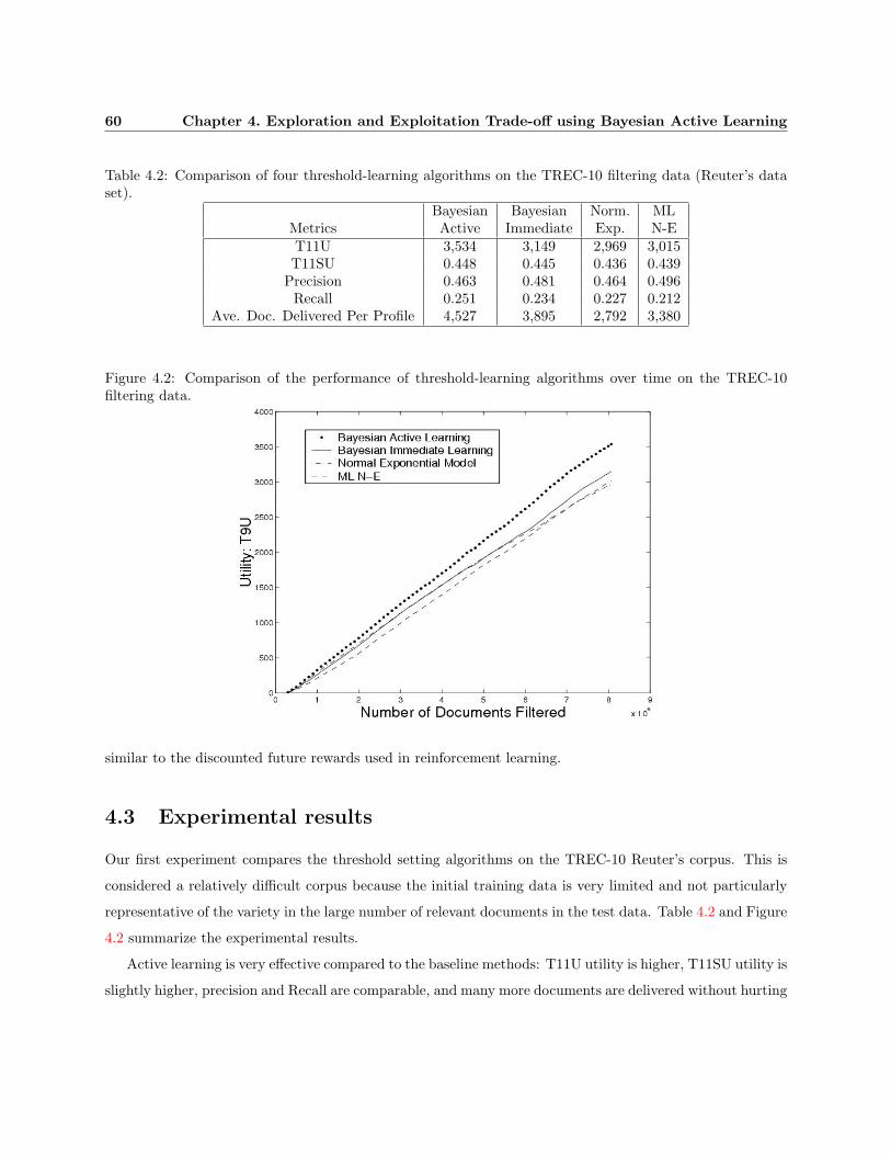
60 Chapter 4. Exploration and Exploitation Trade-off using Bayesian Active Learning
Table 4.2: Comparison of four threshold-learning algorithms on the TREC-10 filtering data (Reuter’s dataset).
Bayesian Bayesian Norm. MLMetrics Active Immediate Exp. N-ET11U 3,534 3,149 2,969 3,015T11SU 0.448 0.445 0.436 0.439
Precision 0.463 0.481 0.464 0.496Recall 0.251 0.234 0.227 0.212
Ave. Doc. Delivered Per Profile 4,527 3,895 2,792 3,380
Figure 4.2: Comparison of the performance of threshold-learning algorithms over time on the TREC-10filtering data.
similar to the discounted future rewards used in reinforcement learning.
4.3 Experimental results
Our first experiment compares the threshold setting algorithms on the TREC-10 Reuter’s corpus. This is
considered a relatively difficult corpus because the initial training data is very limited and not particularly
representative of the variety in the large number of relevant documents in the test data. Table 4.2 and Figure
4.2 summarize the experimental results.
Active learning is very effective compared to the baseline methods: T11U utility is higher, T11SU utility is
slightly higher, precision and Recall are comparable, and many more documents are delivered without hurting

4.3. Experimental results 61
Table 4.3: Comparison of Bayesian active learning and Bayesian immediate learning on one user profile.Bayesian Bayesian
Metrics Active ImmediateT11U 10,488 8,712T11SU 0.296 0.246
Precision 0.682 0.644Recall 0.578 0.509
Ave. Doc. Delivered Per Profile 10,017 9,342
Table 4.4: Comparison of the threshold learning algorithms on the TREC-9 filtering data set (OHSUMEDdata, OHSU topics).
Bayesian Bayesian Norm. MLMetrics Active Immediate Exp. NET11U 11.32 11.54 6.59 11.79T11SU 0.353 0.360 0.329 0.362
Precision 0.300 0.325 0.256 0.339Recall 0.231 0.203 0.264 0.177
Ave. Doc. Delivered Per Profile 31 25 46 20
utility. As expected, the maximum likelihood normal-exponential method, which compensates for sampling
bias, outperforms the basic Normal-Exponential method. Sampling bias is not a problem for discriminative
models, such as the Bayesian active and Bayesian immediate methods. Bayesian active learning outperforms
the other models at all times during the experiment (Figure 4.2).
Comparing the performance of Bayesian active and immediate learning on profiles where active learning
significantly improved performance, we find that active learning increases both recall and precision (e.g.,
Table 4.3). This improvement is partly due to the profile (term and term weight) learning algorithm, which
also benefits from the additional training data generated by the active learner. Our thresholding algorithm
does not consider the benefit of an improving profile, so it is suboptimal (although effective). For simplicity
we have focused only on threshold learning in this section, however the active learning algorithm (Section
4.1) is not restricted to problems of low dimensionality; a higher dimensionality version of the algorithm
could also incorporate profile learning.
The threshold-setting algorithms are also tested on the TREC-9 data set, which contains a relatively small
percentage of relevant documents (0.016%); the test data consists of more than 300,000 documents, but only
an average of 51 documents per profile are relevant. The OHSUMED topic descriptions are well-written,
which provides relatively accurate initial profiles. One might expect that on this data set exploitation would
be much more important than exploration, thus active learning might be detrimental. If the threshold is set

62 Chapter 4. Exploration and Exploitation Trade-off using Bayesian Active Learning
too low, the system delivers thousands of non-relevant documents, hurting utility. In the TREC-9 Filtering
Track evaluations some participants reported negative T11U utility on this data set [119].
The experimental results are summarized in Table 4.4. As expected, active learning does not improve
utility on this data set. More importantly, it does not hurt the utility. Consequently these results rank in
the top 2 when compared with results from the 9 systems that participated in the TREC-9 adaptive filtering
task. ‖
Bayesian immediate learning can be viewed as an active learner that only selects documents on the positive
side of the decision boundary for exploration; Bayesian active learning also samples on the negative side of
the decision boundary. The comparable performance of the Bayesian active and Bayesian immediate learners
indicates that the active learner recognized that the relatively good initial profiles, the limited number of
relevant documents in the stream, and the penalty for delivering non-relevant documents collectively made
exploring the negative side of the decision boundary a poor choice. Active learning does not hurt accuracy,
even in a test where exploration is a risky choice.
4.4 Related work and our contributions
There has been much work on active learning in the machine learning and IR research communities [70, 87,
54, 99]. An active learner selects data to add to its training set so as to learn more about the world with
small amounts of training data. The following three major approaches have used by previous researchers
related to active learning.
Uncertainty of data The uncertainty of the data label(P (relevant|D)), is the focus in this approach. A
filtering systems tends to deliver the documents whose labels the system is most uncertain about. For
example, the “Query by Committee” algorithm selects the next query according to the principle of
maximal disagreement between a committee of classifiers [54]. [99] modified the “Query by Committee”
algorithm with a Naive Bayes model, together with unlabeled data for active learning. [87] introduced
“uncertainty sampling” to choose the instance that current classifiers are most uncertain about. The
underlying assumption of this approach is that the user feedback about the data that the existing
model is most uncertain about can usually help to reduce the uncertainty of the model parameters.
Uncertainty of model The uncertainty of the parameter distribution P (θ|D) is used to measure the qual-
ity of a model, either explicitly or implicitly. A model with less uncertainty is usually better, and
‖This comparison is intended to be descriptive only, because the research community now has greater experience with thisdata set than TREC-9 participants had.

4.4. Related work and our contributions 63
the system usually delivers the document that will produce the best model. [145] provided a theo-
retical framework that uses KL divergence to measure the uncertainty of the model parameters for
active learning and applied it to Support Vector Machine classifiers. [38] used variance of the model
parameters to estimate the uncertainty of the statistical model parameters.
Utility of a model The average utility based on the model parameter distribution (E(U(P (θ|D)))) is used
to measure the quality of a model. A model with a larger expected utility is usually better, and the
system usually delivers the documents that will result the best model. Most of the work in Bayesian
experimental design falls into this category. How to define the utility function is a major research topic
in this area [34], and it is not necessarily the same as the global utility the system wants to optimize.
Unfortunately, most of the prior active learning research, especially that of the first two categories,
focused on interactive retrieval tasks. Thus it often only considered the exploration aspect of the problem,
and did not address the trade-off between exploitation and exploration. These algorithms cannot be applied
easily to adaptive filtering, where the system is evaluated based on utilities such as T11U , and the direct
cost/reward of delivering the document (exploitation) is as important as the improvement in model estimation
(exploration). Especially in the early stage of filtering, if a lot of non-relevant documents are delivered to
the user because the system wants to explore, the user may feel unsatisfied and stop using the system.
There is also much prior research on adaptive filtering and recommender systems. In order to succeed
in practice, most of the prior work focused on exploitation, and little of it addressed the trade-off between
exploration and exploitation. The adaptive filtering community has developed various algorithms for setting
dissemination thresholds, which is vital for the system’s performance. Some researchers also consider the
long term effect of each recommendation. [134] and [26] proposed to use Markov Decision Processes to model
the sequential decision problem in a recommendation system for e-commerce sites. However, a lot of training
is needed to learn their model, thus the approach is more appropriate for collaborative filtering. [33] used
the information gain between a document and the model to select documents, however the task was batch
filtering instead of adaptive filtering, and their approach for combining information gain with the immediate
cost/reward is very heuristic.
Prior research in related areas influenced our work. The Bayesian framework, on which our algorithm
is based, was widely used by Bayesian statisticians [34]. It has been used by computer scientists for active
learning in text classification [145][99]. Our approach falls into the third category listed above, and the main
focus of our work is to derive a utility function: Utility Divergence. Our approach also matches the Risk
Minimization framework described in [78]. The work described in this dissertation differs from prior work
in two major aspects.

64 Chapter 4. Exploration and Exploitation Trade-off using Bayesian Active Learning
• This research uses utility divergence to measure the quality of the model for exploration. Utility
divergence generalizes some already existing measures used for active learning. For example, if the
objective function for a classification system is to maximize the likelihood of the data, utility divergence
becomes KL divergence, which is used to measure the quality of a model in [144]. However, in adaptive
filtering user satisfaction is usually modeled by utility (e.g., Table 2.1), and the system is evaluated
using linear utility. Our algorithm uses utility divergence to measure the quality of the model, thus it
optimizes utility directly, based on the Bayesian framework.
• This research considers the direct and indirect cost/reward for delivering a document. An adaptive
filtering system must consider the immediate cost/credit for a request, that is, it gets credit AR for
delivering a relevant document and penalty AN for delivering a non-relevant document. Previous work
in active learning did not consider this cost/credit, which affects the system performance significantly.
Most of the previous work in adaptive filtering were focused entirely on this cost/credit, disregarding
the future benefit.
To summarize, exploitation and exploration are combined in a single, unified framework based on utility
divergence.
4.5 Summary
A filtering system that tries to explore what users like may be too aggressive and deliver too many non-
relevant documents to the user, while a system that does not explore may be too conservative and perform
poorly in the long run. The filtering solution described in this chapter is developed to avoid both problem.
Based on Bayesian theory, we model the trade-off between exploitation and exploration in adaptive informa-
tion filtering. We view it as a two step message passing process in Figure 4.1. In order to optimize a global
utility function, we have derived a quantitative measure of the immediate cost/reward and future reward of
delivering a document. We believe that this is the first work to study the trade-off between exploration and
exploitation in adaptive information filtering.
The experimental results have demonstrated that Bayesian active learning by combination of exploration
and exploitation can improve results on favorable data set, for example, when the initial profiles are poor
and the document stream contains many relevant documents. The results have also demonstrated that it can
have little effect on unfavorable data set, for example, when the initial profiles are good and the document
stream contains few relevant documents. Bayesian active learning handles both of these situations well,

4.5. Summary 65
exploring only when it is useful to do so. When the algorithm does not explore, it is as good as three
competing methods.
This chapter also answers a common question when people use the Bayesian approach: is it worth mod-
eling the uncertainty of the parameters? Since integration as in Equation 2.12 can be computationally
expensive, maximum a posteriori MAP estimation (MAP) or maximum likelihood estimation (ML) algo-
rithms (Section 2.3.4) are probably preferable to Bayesian averaging if their performance is comparable. In
fact some researchers do think ML or MAP is enough, considering that in some classification tasks, people
do observe comparable performance between these approaches. This chapter has demonstrated that active
learning is one of the problem where modeling the uncertainty of parameters explicitly is necessary for a
principled solution. Existing algorithms that consider exploration benefit while filtering without explicitly
modeling the model uncertainty are heuristic and have to do exploration and exploitation trade-off in an ad
hoc way [33].
There are several directions for further research following the work described in this chapter. The utility
used in this chapter is based on TREC relevancy linear utility evaluation measure, and one future direction
is to use different utility functions, such as a utility measure with discounted future relevant documents
or other criteria beyond relevancy. The research reported here only applied the new framework to setting
dissemination thresholds, however the basic principle of combining expected immediate utility and utility
divergence gain is also applicable to problems of higher dimensionality, for example learning the importance of
features such as words or phrases. The computational method used in this chapter (i.e. approximation based
on sampling using Metropolis algorithm) is tailored for low dimensionality problems. For high dimensionality
problems, approximation based algorithms might be necessary for efficiency concerns. Our model of P (x)
and how the expected number of future documents is estimated are far from optimal, and additional research
in this direction is needed. Utility divergence, the model quality measure derived in this chapter, is very
general and can also be used in many other active learning tasks besides filtering, such as the interactive
retrieval task [136].

Chapter 5
User Study
Traditional adaptive filtering data sets consist of documents, user queries, and assessments of whether a
document is relevant to a user query or not. On the other hand, some prior research work suggests that
more forms of evidence, such as novelty or readability, about the user’s interests and the document content
may be useful [166][39][60][131]. However, the traditional datasets introduced in Section 2.1.2 and used in
the previous chapters don’t support such research. This chapter investigates how to acquire a more detailed
adaptive filtering dataset with multiple forms of evidence. The next chapter explores how Bayesian graphical
models can be used for adaptive filtering research when rich user information is available.
The following sections describe our efforts towards collecting the new adaptive filtering data set. Section
5.1 describes the adaptive filtering system we developed for the user study and Section 5.2 introduces the
subjects participated the study. Section 5.3 describes the data collected, followed by basic statistical analysis
of the data in Section 5.4. Section 5.5 summarizes.
5.1 System description
There were two major goals of the user study. The first goal was to collect an adaptive filtering data set from
a variety of users with explicit feedback, implicit feedback, a wider range of information about documents
and topics, and a heterogeneous set of documents. The second goal was to explore a realistic and relatively
low-cost method of collecting detailed data for adaptive filtering research.
To achieve these goals, we developed a web based news story filtering system (Figure 5.1) located at
www.yow-now.com. This system constantly gathers and recommends information to the users. The system
has six major components: a news crawler, a text indexer, a database server, an adaptive filtering system,
a web server, and a browser. The crawler has about 8000 candidate RSS news feeds to crawl frequently.
RSS is a format for syndicating news and the content of news-like sites [113]. The adaptive filtering system
learns from users’ explicit feedback and recommends documents to the users. An indexer [43] parses each
incoming news story and incrementally builds a text index of documents to facilitate the computation of
66
5.1. System description 67
Figure 5.1: The user study system structure. The structured information, such as userfeedback and crawler statistics, is kept in the database. The content of each web pagecrawled is saved in the news repository.
the filtering system. Users use a special browser modified based on the Curious Browser [37] and log into
the system daily to read and evaluate what the system has delivered to them. The special browser captures
the implicit and explicit user feedback from a user and sends the information to the web server at real time.
The information is saved in a central database and used by the filtering system to learn user preferences.
An example of the web interface after a user logs in is in Figure 5.2. The news on the left column are
the same for all users, while the news on the right column are user specific. The user specific news the
system recommends usually have a long delay, and the user independent news are almost real time with a
few minutes delay. The delay of recommendation may be an issue in a real news filtering system if the goal
is to evaluate the recommendation accuracy of the filtering system, because the value of information drops
quickly over time. However, it is not a serious problem for our task, because the major goal of the study is
to collect data.
The interface also provides some simple search functionalities so that the users can search the articles in
Yow-now’s news archive using keywords and get a list of news, or search the news sources using keywords
and get a list of RSS feeds.

68 Chapter 5. User Study
Figure 5.2: Web interface after a user logs in.

5.2. Subjects 69
Figure 5.3: The interface for users to provide explicit feedback on the current newsstory.
5.2 Subjects
We posted several advertisements about the paid study on the campus of Carnegie Mellon University, and
subjects were chosen based on first come first serve criteria. They are from a variety of programs at Carnegie
Mellon University: Information Systems Management, Business, Electrical and Computer Engineering, Psy-
chology, Art, Mathematics, Professional Writing, Ethics, History and Public Policy, Management, Civil
Engineering, Biological Science, Economics, MBA, Clinical Psychology, Industrial Design, Chemical Engi-
neering, Business and Social History, Computational Finance, and Communication Design. The subjects are
not affiliated with our research otherwise.
A four week time period was selected for this study since it fit the schedule and funding constraints of
the author and also fit the schedule of the participants, who would leave for summer vacation right after the
study. We expected to collect enough data for evaluation over this period of time.
The subjects were required to read the news for about 1 hour on www.yow-now.com web site every day
and provide explicit feedback for each page they visited. In the last week of the study, some subjects read
2 hours per day, although they were encouraged but not required to do so. Subjects were informed during
the recruitment and at the beginning of the study that 1) the study would last for 1 month; 2) they were
required to provide user feedback during the study and the feedback would be logged and made publicly

70 Chapter 5. User Study
available for the research community after anonymizing their identity; 3) each of them would be paid on
hourly basis; and 4) subjects who were unable to finish the first 2 weeks of the study would be paid with state
minimum salary. We considered 15 a reasonable subject number that would generate a significant amount
of data over 4 weeks. We accepted more than 20 subjects initially, considering the possibility of dropout
and our budget constraint. Several subjects dropped out at the first 2 to 3 days without requesting for any
salary, one subject dropped out right after the second week, and 20 subjects finished the study in 4 weeks.
In general, 28 users, including the author and some other researchers interested in the research, tried this
system. However, only 21 users were paid subjects in the user study, including the one who worked only for
2 weeks.
5.3 Data collected
We collected 7881 feedback entries from all 28 users, among which 7839 were from the 21 official participants.
Each entry contains several different forms of evidence about a news story a user clicked and assigned to a
specific topic. ∗
Our intention to collect these forms of evidence is not to be exhaustive, but representative. These forms
of evidence were saved in several tables inside a database or in text files on the server. They can be roughly
classified into the following five categories listed in Table 5.2 to 5.6.
5.3.1 Explicit user feedbacks
The users were required to use a special browser we modified. The browser is based on the CuriousBrowser
developed by [37]. After finishing reading a news story, a user was required to click a button on the toolbar
of the browser to bring up an evaluation interface as shown in Figure 5.3. † Through this interface, the
user provided the explicit feedback about the current story, including the topics the news story belongs to
(classes), how the user likes this news story (user likes), how relevant the news is related to the class(es)
(relevant), how novel the news story is (novel), whether the news story matches the readability level of the
user (readable), and whether the news story is authoritative (authoritative).
The questions were designed to keep the feedback interface easy to understand and reasonably small. We
chose to ask about user likes because it is the most important reason for why a filtering system should or
∗Each entry is for a <document, user topic, time> tuple. Topic usually refers to a class about a specific subject, howeverwe use topic interchangeably with “class” in this chapter.
†The lists of candidate classes on the interface varies for different users. Because users use the system at their own place,we didn’t get a snapshot of their remote machine or regenerate the exact interface. This is a snapshot of the author’s interface.

5.3. Data collected 71
shouldn’t deliver a document to the user. We chose to ask about relevant, novel, readable, and authoritative
because them are possible factor that may influence a user’s rating of the document according to our previous
experience and existing literature ([166][39][76]). The user likes, relevant and novel are recorded as integers
ranging from 1 (least) to 5 (most). readable and authoritative are recorded as 0 or 1. The candidate answers
are more detailed for relevant and novel because of the author’s research focus.
A user has the option to provide partial instead of all explicit feedback because the system is designed
to give them the flexibility, although formal participants were asked to provide all explicit feedback for the
user study. A user can create new classes, and choose multiple classes for one documents. We encouraged
the users to create classes about topics they are interested in, however we also let the users put non-topic
tags, such as “weird story”, using the evaluation interface.
5.3.2 User actions (Implicit feedback)
The browser used was originally designed by [37]. It records some user actions, such as a user’s mouse
activities, scroll bar activities, and keyboard activities (Table 5.3). It sends a record of these actions in
addition to the explicit user feedback to the web server as soon as a user finishes rating a piece of news. The
definition of some of the actions are:
TimeOnMouse how many milliseconds the user spent on moving the mouse
TimeOnPage how many milliseconds the user spent on a page
EventOnScroll the number of clicks on the vertical and horizontal scroll bars
ClickOnWindow the number of clicks inside the browser window but not on the scroll bars
If the left mouse button is pressed down, the browser counts that as one click. When the mouse is out of
the browser window or when the browser window is not focused, the browser does not capture any activities.
More details about the actions are in [84]. These actions are easy to get as implicit feedback from the user.
5.3.3 Topic information
Each participant filled out an exit questionnaire at the end of the user study and answered several topic
specific questions for each of his/her most popular 10 topics and topics with more than 20 evaluated doc-
uments each (Table 5.4, Section 8.2). The questions include how familiar the user is with the topic before
participating in the study (familiar topic before), how much the user likes this topic (topic like), and how

72 Chapter 5. User Study
confident the user is with respect to the answers he/she provided (topic confidence). We include these topic
specific information as evidence, because they may be collected when a topic is created and used while
filtering. Whether collecting them in exit questionnaire affects the answer needs further investigation. More
information about the exit questionnaire is in Section 8.2.
5.3.4 News Source Information
The news stories were crawled from news sources through the RSS. For each RSS feed, we also collected
the number of web pages that link to it (RSS LINK ), the number of pages that link to the server of it
(HOST LINK ), and the speed of the server that hosts it. We collected this information because we felt it
may be related to the authority of a news story.
5.3.5 Content of each document
One very important information source for the filtering system is the content of each document. Our approach
to use the text content is to calculate some representative numbers that characterize the document and use
these numbers as evidence while filtering. For example, the relevance score,‡ readability score, authority
score, and novelty score of a document can be estimated based on user history and the content of the
document. The scores are very different from the explicit feedback (relevant, novel, authoritative, readable),
because the scores can be estimated before delivering a document to a user, while explicit feedback can only
be collected after a user reads a document.
We collected three pieces of evidence to represent the content of each document: the relevance score, the
readability score and the number of words in the document (doc len) (Table 5.6). To estimate the relevance
score of the documents, the system processes all of the documents a user put into a class. These documents
were ordered by the feedback time. The system adaptively learns a LR Rocchio relevance model for each
class using the relevance feedback each user provided §. The relevance score of a document is estimated
using the LR Rocchio model learned from all feedback before the document. The LR Rocchio algorithm
requires Boolean user feedback, while the value of the explicit feedback for the relevance in the user study
ranges from 1 to 5. To train the model, we consider a rating higher than 2.5 as positive, otherwise negative.
A document rated x is considered to be β = |x− 2.5| document(s) during learning. Thus a document with
a extreme rating, such as 5, has a bigger influence on the relevance model.
‡In this user study, this score is intended to be a measure of the topical relevance instead of a more general relevance, whichwe refer to as “user likes”.
§User also put non-relevant documents in a class and gave them low relevance score.

5.4. Preliminary data analysis 73
To estimate the readability score of a document, the system process all of the documents in all users’
classes ordered by the feedback time and adaptively learns a user independent readability model using a
logistic regression algorithm. The readability model is a high dimensional vector of term weights. The
readability score of each <document, user class, time> is estimated using the readability model learned
from all users’ readability feedback before it. It’s worth mentioning that the readability model can be user
dependent in a filtering system. For example, the system may build different readability model for kids in
grade one and college students, because their vocabulary differs a lot [39]. We learned a user independent
readability model in this dissertation because all users were undergraduate or graduate students.
5.4 Preliminary data analysis
This section reports some preliminary statistical analysis on the data collected. The analysis is designed to
address the following questions.
What are the basic characteristics of each variable? We calculate the mean, standard deviation, max
and min, percentage of missing data of each variable. We also plot the histogram and exact value of
some variables.
How informative is one type of evidence if other forms of evidence are not available? We calcu-
late the correlation coefficient between each form of evidence and the user likes feedback.
Is the evidence person/class specific? We compare person/class specific measures of some variables.
Are the data collected reasonable? We compare the measures of some forms of evidence with those
reported by other researchers.
5.4.1 Basic statistics
The basic descriptive statistics of all variables collected are in Tables 5.2 to Table 5.6. The statistics
are calculated over 7881 feedback entries from all 28 users, among which 7839 were from the 21 official
participants. The minimum values, maximum values, means and variances of the different variables are
very different. For example, the mean and variance of TimeOnPages are very large (7.2× 10⁴, 1.3× 10⁵, in
milliseconds), while the means and variances of explicit feedback are much smaller, ranging from 0 to 5.
The values of some evidence may be missing, except for the user actions and news source information that
the system can always collect. Out of the 7991 entries, only 4522 (57%) entries contain no missing value. The

74 Chapter 5. User Study
Figure 5.4: The number of classes each user has created.
missing rate of each form of evidence is also reported in the tables. There are several reasons why the evidence
is missing. For example, the explicit feedback may be missing because users didn’t always follow instructions,
a relevance score may be missing for the first several stories in a class, or the topic familiar before value
for a topic may be missing because of the experimental design (Section 8.2). We think it is common to have
missing data in an operational environment.
More than 700 classes were created by all 28 users. The 21 official participants, one of which quit after 2
weeks, created 680+ classes during the study. Figure 5.4 shows the number of classes created by each user.
On average, each user created 32.5 classes (standard deviation ≈ 26 ). Some users created a large number
of classes. Further investigation of user profiles shows that a single user may have created duplicate classes
such as “Carnegie Mellon Univ” and “Carnegie Mellon University”. There are three possible reasons for
this:
1. The data used to generate candidate classes in user feedback interface in Figure 5.3 were saved on user’s
local machine.¶ A user didn’t follow the instruction to migrate class information from one machine to
another when he/she changed machines;
¶The server also keeps a copy of the classes created by the user, but the browser uses local data to generate the user interface.

5.4. Preliminary data analysis 75
Figure 5.5: The histogram of the number of documents the28 users clicked and evaluated for each class.
Figure 5.6: The histogram of the number of documentsuser clicked and evaluated for each class: X truncated to25.

76 Chapter 5. User Study
class label Count class label Count class label Countdefault 373 experiential 20 Charity 1
familiar topic 256 college 20 court 1U.S. 222 studies conducted 20 Hong Kong 1
world news 180 diet 20 stupid 1science 162 presidential 20 offended 1USA 156 ebay 20 Bangladesh 1
technology 154 SUBJECT Market 19 Food news 1business 150 entertainment 19 Odd stories 1politics 145 design 19 Not so interested 2
Table 5.1: Samples of class labels provided by the users and the number of documents put in each class.
2. When the number of classes is large, the class name list on the explicit feedback interface (Figure 5.3)
is long. Thus the user typed in a class name instead of taking time to find the existing class using the
scroll bar;
3. The user created a class with a typo and then recreated a new one.
Thus we have a comparatively large number of classes per user and a small number of documents per class.
Retrospective analysis suggests that GUI and system design changes could reduce the amount of cases, but
it is unlikely that they could be entirely eliminated from an operational system used by ordinary people.
Systems will always have errors, and people will always make mistakes.
The histogram of the number of documents user clicked and evaluated for each class is in Figure 5.5. To
get greater details on the majority of classes, we truncate the X axis to 25 in Figure 5.6. It shows that about
200 classes have only one document. For these classes, learning class specific models is almost impossible.
Some classes contain more documents. Class specific models, such as a relevance model, for these larger
classes will be more accurate.
Some samples of large, middle and small size classes are listed in Table 5.1. It shows that the classes
are very diverse and of very different granularity. Besides using class labels to represent topics, the users
also used the class labels as comments for documents, such as “not so interested” or “odd stories”. The set
of class is very different from one would normally seen in TREC data, because we have given users a great
deal of freedom to create classes they want to have in their profile online, and we didn’t given them a strict
definition of a class. This suggests that in a real scenario, users may not make interpretations and create
consistent classes on the fly. Although it poses a challenge to a filtering system to learn classifiers with such
diversity, this represents a realistic user scenario.
The label of a large class, such as “USA”, suggests a big universe of relevant documents. However, the
label may not be an accurate description of a user’s information need. As a user’s interest is related to the

5.4. Preliminary data analysis 77
user’s domain beliefs, context and goal, it is not easy for a user to describe what he or she wants exactly
using labels. For example “world news” does not mean that the user wants to read all off the world news,
since there are thousands documents exist on this topic. Users are rather selective and only read a very
small amount of stories every day. The histogram of the variable user likes (Figure 5.9) shows that even for
the stories a user has read, the user may not like it and rates it 1 or 2.
We plot the histogram of some other variables, such as relevant (Figure 5.7), novel (Figure 5.7), readable
(Figure 5.7), authoritative (Figure 5.7), the time spent on a page (Figure 5.8) and how much a user likes a
topic (topic like Figure 5.9). The figures show that the density distribution of these variables are very dif-
ferent. The distributions of the explicit feedback look like Gaussian distributions, while that of TimeOnpage
looks like an exponential function. This information may be useful for us to find a better functional forms
of the conditional probability or potential functions while developing a graphical models.
5.4.2 Correlation analysis
In order to understand how useful each individual form of evidence is if other forms of evidence are not
available, we calculate the correlation between each form of evidence and the explicit feedback user likes.
The correlations between user likes and other forms of explicit feedback are very high (Table 5.2). However,
we can only get implicit feedback after a user reads the document, thus the high correlations do not provide
much information for the system to make a decision before delivering a document.
The correlations between user likes and other forms of evidence are more interesting and useful. The
correlation coefficient between the system’s topical relevance score and user likes is 0.37, the highest among
all types of evidence that the system can get before delivering a document. This is not surprising since system
generated topical relevance score has been used by many filtering systems. However, 0.37 is much lower than
0.73, the correlation between relevant and user likes. Further analysis indicates that the correlation between
relevance score and relevant is 0.45.
The correlations between user likes and the topic information (Table 5.4) are relatively high. This
suggests collecting familiar topic before or topic like in a real filtering system, since they are informative
and collecting them requires little user effort (a user only needs to provide information on the class level
instead of document level). Section 6.2 will show how to use this information with other forms of evidence
in a filtering system.
The correlations between the news source information and user likes are weaker(Table 5.5). The success
of using link based algorithms for authority analysis in the web community ([76][27]) suggests the number
of in-links to a news source RSS LINK may be informative if one wants to predict the authority of a news

78 Chapter 5. User Study
story. However, the correlation coefficient between RSS LINK and authoritative is only 0.1589. We find that
a user may identify a page as not authoritative even when it is from a highly authoritative source, such as
from Yahoo News, although the user also identifies other pages from the same news source as authoritative.
This suggests that some successful web page authority algorithms using hyper links may not be as successful
or sufficient in the news domain.
The correlations between user likes and the user actions (Table 5.3) are even lower (Table 5.2). Some
actions, such as TimeOnPage, are more correlated with user likes than other refined actions, such as Nu-
mOfPageDown. This finding agrees with [37].
5.4.3 User specific analysis
So far, the basic statistics and correlation analysis are user independent. However, users are different. Do the
user actions and ratings differ significantly between different subjects? To answer this question, we carried
out a multiple comparison using one way ANOVA test for each variable to see whether the means of each
variable are the same for different users. Only 17 users with more than 200 feedback entries are included, and
other users are excluded. The visualized result for four representative variables are shown in Figure 5.10 to
Figure 5.13. In these figures, each line corresponds to the first 200 entries of the corresponding user. For any
two users, if their projections on the horizontal axis do not overlap, the means are statistically significantly
different. We can see that the means of the same type of evidence can be very different for different users.
However, the means are not randomly distributed, and some users have similar mean.
5.4.4 Comparison with Claypool’s user study
Did the design of the user study affect the user actions significantly? How would the results vary on
different experimental settings? Will other researchers get similar results in a similar experimental setting
with a different group of users? It is hard to give good answers to all these questions. Fortunately, the
data collected in the user study described in [37] is publicly available. That data set shares some forms of
evidence with our data set. We calculate the basic statistics of the shared evidence on their data set (Table
5.7). Comparing Table 5.7 with Table 5.3, we can see that the basic statistics of our data are not very
different from data set used in [37]. Comparing the “corr” column and “corrYow” column, we find that the
correlation coefficients between each individual action and users’ explicit rating are on similar scale for both
data sets. Other forms of evidence, such as relevant, novel, authoritative and readable were not collected by
[37], thus we can’t compare with.

5.4. Preliminary data analysis 79
Table 5.2: Basic descriptive statistics about explicit feedbacks. RLO and RUP are the lower and upperbounds for a 95% confidence interval for each coefficient.
Variable min max Mean variance corr RLO RUP missinguser likes 1 5 3.5 1.2 1 1 1 0.05relevant 1 5 3.5 1.3 0.73 0.72 0.74 0.005novel 1 5 3.6 1.33 0.70 0.68 0.70 0.008
authoritative 0 1 0.88 0.32 0.50 0.48 0.52 0.065readable 0 1 0.90 0.30 0.54 0.53 0.56 0.012
Table 5.3: Basic descriptive statistics about user actions. The unit for TimeOnPage and TimeOnMouse ismillisecond.
Variable min max Mean variance corr RLO RUPTimeOnPage 1× 10⁴ 56 7.2× 10⁴ 1.3× 10⁵ 0.14 0.11 0.16EventOnScroll 0 93 1 3.6 0.1 0.08 0.12
ClickOnWindow 0 81 0.93 2.5 0.05 0.03 0.07TimeOnMouse 0 3.2× 10⁵ 2× 10³ 5.8× 10³ 0.02 0.002 0.05
MSecForDownArrow 0 1.84 211 882 0.08 0.06 0.10NumOfDownArrow 0 91 1.1 4.7 0.09 0.06 0.10MSecForUpArrow 0 7× 10³ 29 240 0.03 0.004 0.05NumOfUpArrow 0 23 0.10 0.8 0.04 0.01 0.06NumOfPageUp 0 19 0.12 0.9 ' 0 ' 0 v
NumOfPageDown 0 19 0.14 1 ' 0 ' 0 ' 0MSecForPageUp 0 6× 10⁴ 22 202 ' 0 ' 0 ' 0
MSecForPageDown 0 7× 10³ 28 251 ' 0 ' 0 ' 0
Table 5.4: Basic descriptive statistics about topics.variable min max Mean variance corr RLO RUP missing
topic familiar before 0 7 3.6 1.9 0.30 0.28 0.32 0.27topic like 0 7 4.9 2.0 0.30 0.28 0.32 0.27
topic confidence 0 7 4.7 2.0 0.34 0.31 0.36 0.27
Table 5.5: Basic descriptive statistics about news sources. RSS LINK is the number of web pages that linkto the RSS source. HOST LINK is the number of pages that link to the server of the RSS source.
variable min max Mean variance corr RLO RUPRSS LINK 0 1350 90.35 4.89 0.14 0.12 0.17
HOST LINK 0 4.69× 10⁵ 4.41× 10⁴ 7.5× 10⁷ 0.08 0.06 0.10RSS SPEED 0 4.88× 10⁷ 3.92× 10⁵ 3.7× 10⁹ -0.08 -0.10 -0.06
Table 5.6: Basic descriptive statistics about documents. The length of the document does not include HTMLtags.
variable min max mean variance corr RLO RUP missingdoc length 1 44 837 1.2× 10³ 0.04 0.02 0.06 0.05
relevant score 0 1 0.49 0.42 0.37 0.34 0.39 0.18readability score 0.15 1 0.52 0.16 0.25 0.23 0.28 0.11

80 Chapter 5. User Study
Figure 5.7: The histogram of four different explicit user feedback. -1 means the user didn’t provide thefeedback. relevant and novel are recorded as integers ranging from 1 (least) to 5 (most). readable andauthoritative are recorded as 0(negative) or 1(positive).

5.4. Preliminary data analysis 81
Figure 5.8: The histogram of milliseconds spent on a page.
Figure 5.9: The histogram of more variables: user likes, and topic like.

82 Chapter 5. User Study
Figure 5.10: Multiple comparison of the averagetime (in milliseconds) spent on a page for differentusers. Only 17 users with more than 200 feedbackentries are included. Most of the users spent lessthan 100 seconds/page on average.
Figure 5.11: Multiple comparison of the averagenumber of up arrow (↑) usage on a page for dif-ferent users. Only 17 users with more than 200feedback entries are included.
Figure 5.12: Multiple comparison of the averagenumber of down arrow (↓) on a page for differentusers. Only 17 users with more than 200 feedbackentries are included.
Figure 5.13: Multiple comparison of the averageuser likes rating for different users. Only 17 userswith more than 200 feedback entries are included.

5.5. Summary 83
Table 5.7: Basic descriptive statistics about user actions collected by the system used in [37]. corr is thecorrelation coefficient between each form of evidence and the explicit feedback on [37]’s data. corrYow is thecorrelation coefficient between each form of evidence and the explicit feedback user likes on our user studydata.
Variable min max Mean variance corr corrYowTimeOnPage 0 9.6× 10⁶ 4.2× 10⁴ 2.1× 10⁵ 0.1025 0.136EventOnScroll 0 151 1.22 7.38 0.0800 0.103
ClickOnWindow 0 297 2.13 9.96 0.1082 0.054TimeOnMouse 0 7× 10⁵ 6.35× 10³ 2.5× 10⁴ 0.1098 0.024
MSecForDownArrow 0 9.4× 10⁴ 347.75 3.13 0.0645 0.080NumOfDownArrow 0 213 1.1337 8.18 0.0887 0.085MSecForUpArrow 0 4.4× 10⁴ 82.39 1.2× 10³ 0.0356 0.026NumOfUpArrow 0 72 0.17 1.8 0.074 0.037NumOnPageUp 0 12 0.045 0.51 0.05 ' 0
NumOfPageDown 0 15 0.06 0.67 0.045 ' 0MSecForPageUp 0 2.5× 10⁴ 143.72 1.0× 10³ 0.0873 ' 0
MSecForPageDown 0 4.0× 10⁴ 227.8 1.6× 10³ 0.0714 ' 0UserRating 0 5 2.29 1.85 1 1
5.5 Summary
This chapter describes a user study to collect an evaluation data for further research on combining multiple
forms of evidence. It demonstrates that we can build a longer-term learning environment and collect a
significant amount of data about a user’s interests with a reasonably small effort. ‖
We have collected a new evaluation data set that contains thousands of extensive implicit user feedback
(such as a user’s mouse usage, key board usage, document length), explicit user feedback (such as novel,
relevant, readable, authoritative, and whether a user likes a document or not), and other forms of evidence
(such as news source information). The basic characteristics, such as the means, for the multiple forms of
evidence collected are very diverse. Most forms of evidence are correlated with user likes. The correlation
between implicit feedback and user likes is much weaker than that between explicit feedback and user likes.
Compared with data collected by other researchers, this data set looks reasonable.
In general, the user study represents a real world task with a more realistic setting, where users choose
to create their own classes and read news using their own computers at the time and place they want. This
realistic setting enables us to collect a very detailed filtering data set with ordinary people and relatively
available tools. The data is very different and possibly more power than existing filtering data sets created
by NIST for TREC.
‖It used a small budget of about $6000, not including the author’s own stipend covered by a fellowship. The author spentabout 1 month on designing the user study, 1-2 months on implementing and testing the whole system, and 1 month on runningthe user study with the real users.

84 Chapter 5. User Study
The data set is noisy, with many missing entries, and without thorough evaluation for all <document,
user class, time> tuples. It would be relatively easy to create a cleaner data set later, but some of the
characteristics, such as missing entries and diversity of variables, are common in the real world and unlikely
to be eliminated entirely from operational system used by ordinary people.
Because we only collected data for documents a user clicked, the analysis in this section and later sections
only applies to such kind of data. The general statistics and correlation coefficients may be very different for
un-clicked documents. Further study, such as treating un-clicked data entries as entries with missing value
or forcing users to provide feedback for some un-clicked data, is needed to study this problem.
Chapter 6
Combining Multiple Forms of Evidence UsingGraphical Models
We have collected thousands of cases, each of which contains multiple forms of evidence for a <document,
user class, time> tuple. Combining the evidence while filtering is a challenging task, and we need to handle
the diversity of the evidence and various missing data situations.
Researchers have identified three major advantages of the graphical modeling approach: 1) it can naturally
handle situations of missing data based on the conditional dependencies encoded in the graph structure; 2)
it can learn causal relationships in the domain, thus help us to understand the problem and to predict the
consequences of intervention; and 3) it can easily combine prior knowledge, such as partial information about
the causal relationship, with data for learning.
Because of these advantages, we hypothesize: the Bayesian graphical modeling approach is a useful
framework to combine multiple forms of evidence for filtering.
One natural approach is representing the filtering system’s belief about the user based on multiple forms
of evidence as graphical models. The belief can be used in two ways: guiding the system designer’s future
actions (such as deciding whether to collect certain evidence), or directly used in the choice of a system
action (such as deciding whether to deliver a document to the user). To test the hypothesis and explore the
graphical models’ effectiveness in both directions, we carry out several experiments with the data collected
in the user study described in Chapter 5. The experiments were designed to answer the following two specific
questions.
• Can the graphical modeling approach help us to better understand the domain? For example, can the
algorithm tell us what the relationships are between user actions and relevance of a document, how
authority relates to the user preference for the page, whether the usage of a specific keyboard key is
informative, are users differ from each other, and so on. This information may guide us design a better
filtering system.
• Can the graphical modeling approach help us to improve the performance of an adaptive information
85

86 Chapter 6. Combining Multiple Forms of Evidence Using Graphical Models
filtering system? For example, when a document arrives, can we predict a user’s preference for the
document better than using only a topical relevance model? This prediction will be used directly in
deciding whether to deliver the document to the user.
To answer the above questions, we study the three advantages of graphical models in the experiments.
More specifically, to see whether the proposed solution can help us to understand the domain better, we
use the causal graph structure learning algorithms (GM advantage 2), together with some prior knowledge
of the domain (GM advantage 3), to derive the causal relationships between different user feedback, actions
and user context. To see whether the proposed solution can help us to improve an existing filtering system,
especially in the situation of missing data, we use statistical inference tools to predict how much a user likes
a document under different evidence missing conditions (GM advantage 1). Different graphical models are
developed and evaluated for different purposes, either to understand the domain or to improve the prediction
accuracy. Linear regression algorithm with two ways to handle the missing evidence situations are also tried
as alternative approaches to combine multiple forms of evidence.
The following sections describe our efforts toward evaluating graphical models for the task of combining
multiple forms of evidence for filtering. Section 6.1 describes how we use existing graphical structure learning
tools to understand the relationships between various forms of evidence from the data. Section 6.2 explores
how to improve the system performance using multiple forms evidence and various models. Section 6.3
discusses related work. Section 6.4 discusses the limitations of our work and proposes future work. Section
6.5 concludes this chapter.
6.1 Understanding the domain using causal structure learning
The correlation analysis in Section 5.4 is useful and has helped us to get a brief idea about the data collected.
However, in order to better understand the underlying truth of the domain, we need to go beyond correlation
and investigate the potential causal relationships between different variables.
To do that, we first specify N nodes, one for each kind of evidence. The graph structure learning
algorithms introduced in Section 2.3.3 are used to explore the causal relationships between multiple forms
of evidence from the data collected. Causal discovery is hard, or even impossible due to the possibility of
uncollected hidden variables or the inadequacy of the data. Some prior domain knowledge, such as forbidden
edges, required edges or temporal tiers, may help to find the causal structure. To demonstrate how to
use prior knowledge to help structure learning, we specify the prior knowledge developed by the author as
temporal-tier constraints of variables before automatic structure learning.

6.1. Understanding the domain using causal structure learning 87
To generate the temporal tier, we first organize the variables into six tiers manually.
Level 1 topic information (topic info =<familiar topic before>), news source information (RSS info =<RSS link,
host link>) and document length (doc len);
level 2 hidden variables, such as relevant novel authoritative and readable, that may affect a user’s prefer-
ence for a document;
Level 3 system generated scores, such as topical relevance score and readability score;
Level 4 user explicit feedback on relevant, novel, authoritative, and readable;
Level 5 user judgment of user likes;
Level 6 user actions, such as milliseconds spent on a page (TimeOnPage) or the number of clicks on the ↓
key (NumOfDownArrow).
We assume users provided accurate judgment about the hidden variables as explicit feedback, thus a
user explicit feedback is always the same as the corresponding hidden variable on level 2. Based on this
assumption, we merge the corresponding nodes on level 2 and level 4 to form a 5-tier as shown in Figure 6.1.
This informs the learning algorithm that a causation (indicated by →) from a higher level to lower level is
prohibited.∗ Although the prior knowledge is engineered by the author and is not guaranteed to be true, it
may help the structure learning algorithms by using the constraints to make the search space smaller.
We also tried a different prior by organizing the variables into 2 tiers, with user likes on level two, while
the other forms of evidence on level one. Moving from a 5-tier prior to a 2-tier prior, we are changing
our prior constraints and making different assumptions about the true causal relationships between these
variables. This helps us to see what the algorithm can learn from a different prior and what kind of causal
relationships are less sensitive to the choice of priors.
There are many graph structure learning packages to generate the graph topology from data [36][133]
[107] [46][4][112]. This section reports the results generated by the PC and FCI algorithms implemented in
Tetrad [133]. We chose these algorithms because they are basic algorithms for causal discovery that work
well with a comparatively small number of nodes and the Tetrad package provides the functionality that
enables us to specify prior knowledge/constraints as a temporal order.
It is very encouraging to see that the structure learned automatically using PC algorithm looks reasonable
(Figure 6.2). According to Figure 6.2, whether a document is novel, relevant, authoritative, readable and
∗X → Y means X is a direct cause of Y.

88 Chapter 6. Combining Multiple Forms of Evidence Using Graphical Models
Figure 6.1: Prior knowledge as temporal tier of variables before automatic structure learning. This priorknowledge informs the learning algorithm that a causation (indicated by →) from a higher level to lowerlevel, such as relevant is a direct or indirect cause of RSS info (relevant→ RSSInfo), is prohibited.

6.1. Understanding the domain using causal structure learning 89
Figure 6.2: A user independent causal graphical structure learned using PC algorithm. The learning algo-rithm begins with the 5 tier prior knowledge. In the causal graph, X − Y means the algorithm cannot tellif X causes Y or if Y causes X. X ←→ Y means the algorithm found some problem. The problem mayhappen because of a latent common cause of X and Y, a chance pattern in a sample, or other violations ofassumptions.

90 Chapter 6. Combining Multiple Forms of Evidence Using Graphical Models
Figure 6.3: A user independent causal graphical structure learned using PC algorithm. The learning algo-rithm begins with the 2 tier prior knowledge.

6.1. Understanding the domain using causal structure learning 91
Figure 6.4: A user independent causal graphical structure learned using FCI algorithm. The learningalgorithm begins with the 5 tier prior knowledge. X → Y means X is a direct or indirect cause of Y. X ↔ Ymeans there is an unrecorded common cause of X and Y. “o” means the algorithm cannot determine whetherthere should or should not be an arrowhead at that edge end. An edge from X to Y that has an arrowheaddirected into Y means Y is not a direct or undirect cause of X.

92 Chapter 6. Combining Multiple Forms of Evidence Using Graphical Models
whether a user is familiar with the topic before using the system (familiar topic before) are direct causes of
the user’s preference for a document (user likes). How familiar with this topic a user is before participating
the user study (familiar topic before) and the number of web links to the news source (RSS LINK ) or host
(host linke) indirectly affect the user’s preference for a page through relevant and authoritative. relevant,
authoritative, familiar topic before and host link influence a user’s actions, such as the number of events on
scroll bars (EventOnScroll).
Comparing Tables 5.3 to 5.6 with Figure 6.2, one may ask why some variables are correlated with user
likes although there are no direct links between them and user likes. For example, why is the correlation
between relevance score and user likes 0.39, while there is no direct link between them? Does Figure 6.2
contradict Table 5.6? The answer is “no”. As no direct link means relevance score is not a direct cause/result
of user likes. The subgraph user likes ← relevant → relevance score means relevance score and user likes
share a common cause of relevant. The correlation between relevance score and user likes is due to the
indirect causal relationship between them. Similarly, several variables are correlated with user likes but
have no direct link to the node user likes (Section 5.4.2).
Although we are using different structure learning algorithms (PC vs. FCI) and different priors (2-
tier vs. 5-tier), the structures learned share some common properties (Figure 6.2, Figure 6.3 and Figure
6.4). For most variables, except the refined actions about specific keys on the keyboard, the length of the
shortest path from the same variable to the user likes node in different structures are similar. For example,
on all figures, the node user likes is directly linked to or from authoritative, relevant, novel, readable and
familiar topic before.
Most of the refined actions, such as the number of times the page up key was pressed (NumOfPageUp),
are several steps away from user likes. In Figure 6.4, there is no path from some refined action nodes to
user likes. This implies that these refined actions are less informative if we want to use the learned model
to predict whether a user likes a document or not. This finding agrees with [37] and Table 5.3.
The node authoritative is directly linked to readability score and host link. The link between host link
and authoritative confirms the existing approaches that use the web link structure to estimate the authority
of a page [76]. The links between readability score, readable and authoritative are very interesting. They
suggest the difficulty to understand a page may make the user feel it is not authoritative. Further investigation
shows that although the percentage of un-authoritative news is less than 15% in general, among the 187
news stories some users identified as “difficult” using class labels, 73% were also rated not authoritative.
Besides some successful web page authority algorithms that only use hyperlinks, the estimation of authority
may be further improved using the content of a page.

6.1. Understanding the domain using causal structure learning 93
variable relevant novel authoritative readablerelevant 1 0.69 0.4328 0.48novel 0.69 1 0.4381 0.49
authoritative 0.43 0.44 1 0.61readable 0.48 0.49 0.61 1
Table 6.1: The correlation coefficient between explicit feedback.
All figures contain links among the four nodes relevant, novel, readable and authoritative. Further analysis
show that the correlation between each pair is high (Table 6.1). Although the algorithms failed to tell the
causal directions between some pairs of variables and disagree with each other about the directions of
certain links, they suggest that the four variables influence each other one way or another. For example,
the readability of a document may influence the user’s evaluation of authority, while whether a document is
relevant or not may influence a user’s evaluation of novelty. There are two possible explanations: 1) this is
an inherent property of the document; or 2) a user is likely to rate one aspect of the document higher than
he should if the other aspects are good.
One may ask why the structure in Figure 6.2 contains no link between readable and readability score,
since there is a causal relationship between the two intuitively. To answer this question, one needs to
understand that the causal relationships learned automatically are what the algorithm “believes” based on
the evidence of the data, the assumptions it makes, and the prior constraints we engineered. The relationships
learned may contain error, because the data are noisy, or the assumptions and the prior constraints may be
wrong. For example, the PC and FCI algorithms do statistical test about the independence relationships
among variables using the data and the final results are subject to the error of the statistical test. The PC
algorithm assumes no hidden variables. However, in additional to relevant, novel, authoritative, and readable,
other hidden variables, such as whether a document is up-to-date, interesting, misleading, etc. [131], may
exist and influence a user’s preference for a document. Thus it is not surprising that some of the causal
relationship, such as the link between readable and readability score is missed in the final graph because of
the limitation of the learning algorithms. The models learned merely shed some light on the relationships
between the variables instead of uncovering the whole truth. It only serves as a starting point for us. To
further understand the domain, we may want to break down some variables in the current graph further and
relate them to either the user or document properties. In general, causal discovery is inherently difficult and
far from solved.

94 Chapter 6. Combining Multiple Forms of Evidence Using Graphical Models
6.2 Improving system performance using inference algorithms
In the previous section, graphical model structure learning algorithms helped us to understand the relation-
ships between variables in the domain better. However, improving system performance to serve the user
better is the primary goal. This section explores how to do that using graphical models. More specifically,
we focus on addressing the following questions.
1. Can the graphical model combine multiple forms of evidence and handle missing data scenario?
2. How well does the graphical modeling approach work compared to some other straightforward ap-
proaches, such as linear regression?
3. Is going beyond topical relevance to combine multiple forms of evidence better than the traditional
relevance filtering?
4. Can we develop a filtering system that works reasonably well with limited user supervision?
5. Are user actions useful for the system given other information?
6.2.1 Experimental Design
Comparison of Graphical models
To answer these questions, several graphical models are created to combine multiple forms of evidence to
predict user preference (user likes). Each graphical model is uniquely defined by the graph structure and a
set of local conditional probability functions or potential functions, both of which can be specified manually
or learned from the data.
To derive the graph structure, we may want to use the causal structures learned in the previous section.
However, using these structures for inference directly is hard because of the circles and a mixture of directed
and undirected links on the graph. Instead, we tried the following directed acyclic graphical models:
GM complete, an almost complete Bayesian network: In this graph, we order the nodes from top to
bottom, and the parents of a node are all the nodes above it, such as in Figure 6.5. For this structure,
the order of the nodes is not very important when using Gaussian distributions.
GM causal, a graphical model inspired by causal models: We manually modify the causal structure
in Figure 6.2 to make it a directed acyclic graph. This gives us the causal graph structure in Figure
6.6.

6.2. Improving system performance using inference algorithms 95
Figure 6.5: Graph structure for GM complete. In these graphs, RSS info={RSS link, hostlink} and Topic info={familiar topic before, topic like} are 2 dimensional vectors repre-senting the information about the news source and the topic in Table 5.5 and Table 5.4.actions=<TimeOnPage,...> is a 12 dimensional vector representing the user actions in Table5.2. user likes is the target variable the system predicts.

96 Chapter 6. Combining Multiple Forms of Evidence Using Graphical Models
Figure 6.6: Graph structure for GM causal.
Figure 6.7: Graph structure for GM inference.

6.2. Improving system performance using inference algorithms 97
GM inference We manually modify the structure in Figure 6.3 to make it a directed acyclic graph, and
result in Figure 6.7. We call it GM inference because the structure looks like an inference graph.
To derive the local conditional probability functions, we need to choose a specific form of the conditional
probability function associated with each node. However, it is very difficult to find a good form that is close
to the real distribution and mathematically tractable while doing inference. For simplicity, we use Gaussian
distributions. If the parents of node X are nodes Y = (Y1, Y2, ...), then P (X|Y ) = N(m+W × Y,Σ), where
N(µ,Σ) is a gaussian distribution with mean µ and covariance Σ. This is a commonly used distribution for
continuous valued nodes. We choose it because of the mathematical convenience, the existence of efficient
learning and inference algorithms for Gaussian networks, and the availability of modeling tools.
Given a graph structure and a specific form for each conditional probability function, the learning algo-
rithm learn the parameters of the functions from the training data.
Baseline algorithms
To answer the second question and tell how well the graphical modeling approach works compared to some
straightforward approaches, we tried an alternative approach to combine multiple forms of evidence: using
linear regression. Linear regression models can’t handle missing values, so we tried two special methods
to solve this problem: 1) building a model that does not use the evidence that is missing for each missing
situation (LR different); or 2) mean substitution: replacing each missing value for an evidence with the
average of the observed evidence (LR mean). For K different forms of evidence, the system may need
to handle 2K different evidence missing situations. A large number of linear regression models need to
be learned if we use the first approach, considering that K is higher than 15 in some of our experiments.
Building 215 models is almost impossible for us, so a heuristic approach, which is discussed later, is used to
make the experiments possible.
We chose this algorithm because the linear regression assumes that the conditional probability distribution
P (y|X) is a Gaussian distribution, where y = user likes and X is a vector with each dimension for a form
of evidence. This assumption matches that of the Gaussian network. Thus the major difference between LR
models and graphical models is due to the structure instead of the functional form.
Different evidence missing situations for testing
Each algorithm is tested at various evidence missing situations. It is difficult to evaluate algorithms under
2K different evidence missing situations. Instead we design the experiments as follows to analyze several
situations of interest.

98 Chapter 6. Combining Multiple Forms of Evidence Using Graphical Models
Depending on the property of the multiple forms of evidence, we first manually grouped them into seven
sets: relevance score, readability score, topic info, RSS info, user actions, explicit feedback, and user likes.
The first four categories may be available before delivering a document to the user, thus can be used by the
system to predict user preference for a document while making filtering decisions.
To answer the third question and tell whether going beyond topical relevance to combine multiple forms
of evidence is better than the traditional relevance filtering, we rank the first 4 sets of evidence according to
the max correlation coefficient between the variables in a category and the user likes. The order is: relevance
score, readability score, topic info, RSS info. A model first predicts the value of user likes given only the
value of the first evidence (relevance score) at testing time. Then more forms of evidence are added in order
to see whether the prediction performance increases.
To answer the fourth question and tell whether we can develop a filtering system that works reasonably
well with limited user supervision, we manually rank the first 4 sets of evidence according to how easy it
is to collect the evidence. The order is: RSS info, readability score, topic info, relevance score. A model
first predicts the value of user likes given only the value of the first evidence (RSS info) at testing time.
Then more forms of evidence are added in order to see whether the prediction performance increases as more
“costly” evidence is available.
To answer the fifth question and tell whether user actions are useful for the system given other information,
we compare each model under two conditions:
without actions a model predicts the value of user likes given the values of the first four sets of evidence
with actions a model predicts the value of user like given the first five sets of evidence, including user
actions.
Implementation issues
We develop the experiments with the BNT Toolbox [107]. The maximum likelihood estimations of the
parameters (m,W,Σ) are learned from training data using EM algorithm and junction tree inference engine
[42] over the graphical models.
In this task, the value of each variable is continuous and normalized to variance one. Each model is
learned using all information available on the first 2/3 of the cases, and tested on the remaining 1/3 of the
cases.
Not all 7991 cases collected in the user study are used in the experiments. We conducted two sets of
experiments. For the first set of experiments, we use 7952 cases where the value of user likes is not missing.

6.2. Improving system performance using inference algorithms 99
For the other set of experiments, we only use 4522 cases where none of the evidence is missing. The results
on the first set of runs are analyzed first, followed by a briefly discuss of the results of the second set of runs.
All graphical models and LR mean model are trained with all types of evidence/features, and the learned
models are independent of the testing conditions. For LR different, we build one model per testing con-
dition and only use features available under the testing condition. However, on the first set of runs using
7952 cases, the training data and testing data contain cases where a piece of evidence that is supposed to
be available is missing. These cases in training data are ignored by LR different and not used to learn
the linear model. However, ignoring these cases in testing data makes cross comparison of testing conditions
difficult, because ignored cases depend on the testing condition. So we use mean substitution approach to
fill the required missing features in testing data while using LR different.
Evaluation measures
The correlation coefficient between the predicted value of user likes and the users’ explicit user likes feedback
is used as an evaluation measure. The baseline method is using relevance score alone.
A linear utility measure is also used. However, the commonly used TREC style linear utility measure
(Equation 2.3) can’t be used here directly, because it focuses only on topical relevance and is defined over
Boolean user feedback. We also consider other aspects of a document now, such as novelty, readability and
authority. The system should get a credit for delivering a document that the “user likes” a lot, and get
a penalty for delivering a document that the “user dislikes”, such as a relevant but redundant document.
Furthermore, how much a user likes a document is represented as a number from 1 to 5 instead of a binary
value. Thus we modify the TREC style linear utility to get a new evaluation measure for user satisfaction
as follows:
Utilityuser likes =5∑
i=1
AiCi (6.1)
This measure is very similar to the linear utility measure defined in Equation 2.3 . It corresponds to
assigning a positive or negative value to each element in the categories of Table 6.2. In our experiments, we
set (C1, C2, C3, C4, C5) = (−1.5,−0.5, 0.5, 1.5, 2.5). If a filtering system delivers a document to a user and
the user feedback of user likes is x, the system receives a value that equals to (x-2.5).
6.2.2 Experimental results and discussions
Figure 6.8 shows the performance of three algorithms on all 7952 cases. The horizontal axis indicates different
testing conditions. The vertical axis is the correlation coefficient between the predicted value of user likes

100 Chapter 6. Combining Multiple Forms of Evidence Using Graphical Models
Figure 6.8: Comparison of the prediction power of different models: forms of ev-idence ordered by correlation coefficient. From left to right, additional sources ofevidence are given when testing. “+RSS info” means the values of news sourceinformation (RSS info) are given besides the value of relevance score, Topic Info,and readability score.
Figure 6.9: Comparison of the prediction power of GM complete at different missingevidence conditions: forms of evidence ordered by user effort involved.

6.2. Improving system performance using inference algorithms 101
User like rating 1 2 3 4 5Delivered A1, C1 A2, C2 A3, C3 A4, C4 A5, C5
Not Delivered 0 0 0 0 0
Table 6.2: The values assigned to documents with different user likes ratings. A1, A2, A3, A4, and A5
correspond to the number of documents that fall into the corresponding category. C1, C2, C3, C4 and C5
correspond to the credit/penalty for each element in the category.
using the model and the users’ explicit feedback provided by the users.
The results show that GM complete performs similarly to LR different. This is not surprising. The-
oretically, if there is no missing entries in training data, GM complete’s estimation of the conditional dis-
tribution of P (user likes|available evidence) would be the same as that of LR different on a testing case
with missing evidence.
LR different and GM complete performs reasonably well given only relevance score. This is not sur-
prising, since it is well known in the filtering community that the system can improve its performance on
future documents with explicit feedback from users on old documents, and existing filtering systems usually
use some measure of topical relevance to make decision. It is encouraging to see that as we go beyond topical
relevance by adding topic info, and readability score, the system keeps improving, and the improvement is
statistically significant. However, there is no obvious improvement after adding RSS info.
One may feel surprised that the correlation coefficient is negative while using LR mean under the “rel-
evance score” condition. Further analysis shows that this evidence is considered unimportant given explicit
feedback, thus the learning algorithm assigns a near zero weight, which by chance is negative, to “relevance
score”. In other words, LR mean gave explicit feedback too much weight and overlooked other evidence. Let
user likes = a+ bX + e, where the X is other evidence except “relevance score”, a and b are the regression
weights, and e is the regression “residual”. Further investigation show that the 95% confidence interval of the
correlation coefficient between e and “relevance score” is [-0.045 0.008]. Thus it is not surprising that “rele-
vance score” has a small negative weight. At testing time, it did not handle the problem of missing explicit
feedback well and the negative weight of “relevance score” dominates. Although GM complete also gave
very high weights to explicit feedback, it could infer the missing values based on other available evidence at
testing time, and thus it performed better than LR mean. LR different does not consider explicit feedback
for training, thus it overlooks other evidence and suffered less from the problem. LR mean may improve if
explicit variables are not included, however it is not a good algorithm to combine multiple forms of evidence
if there is a large variance on how informative each evidence is, since it will suffer from a similar problem
if some strong evidence is missing due to the same reason. GM complete builds a single model to handle

102 Chapter 6. Combining Multiple Forms of Evidence Using Graphical Models
various evidence missing situations, while LR different builds several models, one for each situation. As
we mentioned before, there are 2K different possible evidence missing combinations, and 2K linear regression
models are needed in order to handle all these situations using LR different approach. When K is big,
GM complete may be preferable because it requires less computation and space while performs equally well.
When we order the evidence by the user efforts involved (Figure 6.9), we find that 1) adding “RSS info”,
“readability score” and topic info improves the performance of the system; and 2) the performance under
the “+topic info” condition in Figure 6.9 is close to the “relevance score” condition in Figure 6.8. This
experiment was conducted over documents that the user had clicked after seeing their titles. Because most
of the clicked documents were somewhat relevant (Figure 5.5), the effect of relevance score is not strong in
this experiment. However, this experiment demonstrates the impact and the relative impact of other forms of
evidence, such as “RSS info”. It’s interesting to see that topic familiarity is a factor that influences the user’s
rating of a document. The fact that adding “RSS info”, “readability score” and “topic info” improves the
performance may be extended to un-clicked documents and help the system make better recommendations
than without using the information. However, the degree of the improvement on un-clicked documents may
be different. This result demonstrates how “cheap” information can help to predict whether a user likes a
document he/she clicked. This will directly benefit systems for personal information retrieval and re-use[48],
since little user supervision is needed to train a model to work under the “+topic info” condition in Figure
6.9.
So far, the only graphical model that has been evaluated is GM complete. How about other graphical
models? Will a model with different structure perform differently? Figure 6.10 compares several graphical
models. GM causal and GM inference perform worse than the simple GM complete. Why do struc-
tures that look more causally reasonable not perform as well as the simple GM complete on this data set?
GM complete only assumes the joint distribution of all variables is multivariate Gaussian. GM causal and
GM inference make much stronger assumptions by removing some links between variables, thus putting
independence constraints while learning the models. As we discussed before, the causal relationships learned
automatically are not perfect, thus the constraints imposed by GM inference and GM causal may be
wrong. As a result, they performed worse than a GM complete.
Are user actions useful for the system given other information? We compared each model under two
conditions: with and without user actions (Table 6.3). For each model, there is no statistically significant
difference after actions are added. This means that given other forms of evidence (RSS info, topic info,
relevance score and readability score), the system didn’t improve its prediction much by observing actions
after a user reads the document. However, it does not mean the actions are useless if we learn user specific

6.2. Improving system performance using inference algorithms 103
Figure 6.10: Comparison of the prediction power of different graphical models: forms of evidence orderedby correlation coefficient.
Model Actions added corr RLow RUpLR mean no 0.278 0.243 0.313LR mean yes 0.265 0.229 0.300
LR different no 0.437 0.406 0.468LR different yes 0.438 0.406 0.468GM simple no 0.289 0.253 0.323GM simple yes 0.270 0.234 0.305
GM complete no 0.425 0.393 0.456GM complete yes 0.432 0.400 0.462GM causal no 0.308 0.273 0.342GM causal yes 0.309 0.274 0.343
GM inference no 0.343 0.309 0.376GM inference yes 0.343 0.308 0.376
Table 6.3: A comparison of effect of adding user actions. “relevance score”, “readability score”, “RSS info”and “topic info” are given before actions where added. The data entries with missing value are also used fortraining and testing. corr is the correlation coefficient between the predicted value of user likes using themodel and the true explicit feedback provided by the users. RLO and RUP are the lower and upper boundsfor a 95% confidence interval for each coefficient.

104 Chapter 6. Combining Multiple Forms of Evidence Using Graphical Models
model, or if other forms of evidence (such as relevance score) are not available.
So far, all results are based on 7952 cases where some evidence may be missing. Table 6.4 reports
the results on a second set of runs with 4522 cases where no evidence is missing. The results show the
performance of GM causal and GM inference changes a lot using this new evaluation data, significantly
better than before (Table 6.3). This suggests that we need to be very careful with the structures while
using the graphical modeling approach, since a structure that looks more reasonable may work poorly on
the inference task. However, we couldn’t draw any conclusion on whether GM complete is better in general,
because the answer may be different with different conditional probability distributions, different data sets,
or a better structure learning algorithm.
Will a filtering system that combines multiple forms of evidence using graphical models help us to build
a better practical filtering system that serves the user better? Does a higher correlation between the user’s
explicit feedback on “user likes” and the predicted values mean higher utility?
To answer these questions, we also use the linear utility measure (Equation 6.1) to evaluate the proposed
solution. Ideally, we need to have a thorough evaluation data similar to TREC filtering data, but with
multiple forms of evidence. Unfortunately, it is extremely hard to collect such kind of data. Instead, we use
all <document, user class, time> tuples with user feedback. The first 2/3 of the cases are used as training
data, and the remaining 1/3 of the cases are testing data. The system processes each tuple <document d,
class c, time t> in the testing set ordered by time, and decides whether the document d should be delivered
to the user class c at time t. Delivering all documents in the testing data to the user gives a utility of 2881.5,
which is very high. It is not surprising considering this is a very biased evaluation data set and all testing
data are documents already clicked by the user. The highest possible utility on the testing data is 3300.
We compare three approaches.
LR Rocchio The system delivers the documents to the user if and only if the estimated relevance score is
higher than 0.5. The relevance score is the same as used before (Section 5.3.5). For a <document, user
class, time> tuple missing relevance score, the system does not deliver it.
LR Rocchio + linear regression The system corrects the bias caused by the difference between “user
likes” and “relevance score”. It uses either linear regression to predict “user likes” using “relevance
score”, and delivers the documents to the user if and only if the estimated user likes is higher than 2.5.
GM complete + multiple forms of evidence For each incoming document in the test stream, the sys-
tem uses GM complete to predict user likes given RSS info, readability score, topic info and relevance
score. Then the system delivers the document to the user if and only if the estimated user likes value

6.2. Improving system performance using inference algorithms 105
Model Condition corr RLow RUpLR mean RSS info 0.0316 -0.0192 0.0822
LR different RSS info 0.0316 -0.0192 0.0822GM complete RSS info 0.0316 -0.0192 0.0822GM causal RSS info 0.0316 -0.0192 0.0822
GM inference RSS info 0.0316 -0.0192 0.0822LR mean +readability score 0.1467 0.0967 0.196
LR different +readability score 0.1365 0.0864 0.1859GM complete +readability score 0.1365 0.0864 0.1859GM causal +readability score 0.0648 0.0141 0.1151
GM inference +readability score 0.146 0.0959 0.1953LR mean +topic info 0.2435 0.1952 0.2906
LR different +topic info 0.2875 0.2402 0.3333GM complete +topic info 0.2875 0.2402 0.3333GM causal +topic info 0.2572 0.2092 0.304
GM inference +topic info 0.2303 0.1817 0.2778LR mean +relevance score 0.1284 0.0782 0.178
LR different +relevance score 0.4109 0.3679 0.4522GM complete +relevance score 0.4109 0.3679 0.4522GM causal +relevance score 0.4106 0.3675 0.4519
GM inference +relevance score 0.4189 0.3762 0.4599LR mean +actions 0.1075 0.0571 0.1574
LR different +actions 0.4184 0.3756 0.4594GM complete +actions 0.4184 0.3756 0.4594
GM causal +actions 0.3789 0.3346 0.4215GM inference +actions 0.4424 0.4006 0.4823
LR mean +explicit feedback 0.7396 0.7157 0.7617LR different +explicit feedback 0.7396 0.7157 0.7617GM complete +explicit feedback 0.7396 0.7157 0.7617GM causal +explicit feedback 0.7449 0.7214 0.7666
GM inference +explicit feedback 0.7449 0.7214 0.7666
Table 6.4: A comparison of different models: no missing value cases, coefficient measure. RLO and RUP arethe lower and upper bounds for a 95% confidence interval for each coefficient.

106 Chapter 6. Combining Multiple Forms of Evidence Using Graphical Models
Table 6.5: A comparison of different models: all cases, utility measure. If we deliver all documents in thetesting data to the user, the utility is 2881.5. The highest possible utility on the testing data is 3300.
model evidence utilityLR Rocchio relevance score 2036
LR Rocchio + linear regression relevance score 2750GM complete multiple forms of evidence 2953.5
is higher than 2.5.
Table 6.5 shows that combining multiple forms of evidence achieved a much higher utility using relevance
score only. Although the experimental setting is far from real because the evaluation data are biased,
the graphical model with multiple forms of evidence is more likely to perform better than using relevance
information alone in a real scenario.
It is encouraging to see that GM complete performs better than delivering all documents the users
clicked. One may feel a little surprised to see that the relevance model performs even worse than delivering all
documents to the user, considering relevance models usually perform much better than delivering everything
on TREC data. There are two reasons: 1) delivering everything is already a very high baseline because the
evaluation data only includes documents clicked by the users; 2) the system could not estimate the relevance
score for all <document, user class, time> tuples, especially for the first one or two documents in a user
profile .
It is worth mentioning that all the inference tasks only considered <document, user class, time> tuples
that corresponds to documents users clicked and assigned class labels. The performance may be different on
arbitrary tuples in a real system. A practical filtering system may ask users to create classes manually, or
automatically create user classes and assign documents to classes.
6.3 Related work and further discussion
There is much related work on using implicit feedback in the information retrieval community and user
modeling community. [75] provides a review and classification of works in these areas according to the
behavior category and minimum scope. The prior work suggested many possible behaviors (view, listen,
scroll, find, query, print, copy, paste, quote, mark up, type and edit) on different scope (segment, object and
class) for system designers to choose from. The user actions we collected are based on [37].
There is some early work on news filtering [81][13][47][62]. [32][79][104]. [24] build a personal news
agent that used time-coded feedback from the user to learn a user profile, however their way of integrating

6.3. Related work and further discussion 107
time as feedback is rather heuristic. [106] investigated implicit feedback for filtering news group articles.
They discovered that articles readers spent viewing more than 20 seconds as positive feedback can produce
better recall and precision in filtering than user’s explicit rating. [152] observed incompatible context, noisy
context and incomplete query problems in contextual retrieval applications and developed specific models
to solve these problems. The approach described in this chapter can handle these problems in a unified
framework. There is also much related work on using implicit feedback to improve web retrieval performance
[153][9][141]. We notice a recent independent work using a different kind of graphical modeling approach,
dependency networks, to discover the relationships between implicit measures and explicit satisfaction, and
using decision tree for prediction ([53]). They were focusing on predicting user satisfaction with web search
results based on implicit measures gathered while users were conducting their searches and viewing results.
Their findings justify the graphical modeling approach’s effectiveness in web search task, a task close to
filtering. Our work differs from the previous work in the goal of the task, the range of evidence considered,
the modeling approach we took, and the findings reached.
Different graphical models, such as Bayesian networks, dependency networks, inference networks, and
causal models, have been used to model computer software users [64], car drivers [114], students [41], and
other social phenomena [101]. Choosing graphical modeling as a unified framework to combine multiple
forms of evidence is motivated by these prior work. Our work differs from the previous work because we
are working on filtering, a different task. Moving to the specific domain of information filtering, we have
performed a detailed user study with human subjects at the early stage of the research. In the later stages of
this research, we have used basic statistical analysis techniques and existing graphical modeling algorithms
to understand the data collected and explore how to improve the system performance. More specifically, we
have focused on the missing data problem, which becomes more important as more forms of evidence are
added.
There is much work about how to handle missing data [89]. [129] gives an overview of the state of art.
The approaches to handle missing data can be classified into four categories:
case deletion This approach is the simplest approach and is used by default in many statistical programs.
It can be further divided into two categories: 1)complete case analysis that only uses cases that have
observed values; 2)available case analysis that estimates different parameters using different sets of
samples.
dummy variable coding When the variable is a categorical value, this algorithm creates a new class “not
available” and assign this class label to a missing entry. For a learning algorithm, missing data cases
no longer exist.

108 Chapter 6. Combining Multiple Forms of Evidence Using Graphical Models
maximum likelihood estimation The algorithm fills in the missing entry using the maximum likelihood
estimation of that value. Although the principle of this approach is very simple, but the actual solutions
can be very different and computationally expensive, depending on the models the system use to model
the variables. Except for some special models, there is no closed form solution for ML estimation and
EM algorithm is often used [49].
multiple imputation The algorithm generates multiple imputed values for a single missing entry on the
basis of existing data and using those “imputed” values in the solution [130].
In this dissertation, LR mean models the missing variable as a Gaussian distribution and uses the maximum
likelihood estimation, the unconditional mean of the variable, to replace the missing value. LR different
and GM complete model the joint distribution of all variables as Gaussian distribution and uses the maxi-
mum likelihood estimation, the conditional mean of the variable, to replace the missing value. Besides the
algorithms we tried in this dissertation, other approaches exist to handle the missing value. For example,
regression trees can use “surrogate splitters” to split data if a primary splitter is missing. This allows cases
with different data patterns, including missing pattern, be handled differently. GM complete may not be the
best approach for the task, but it is a rather natural solution under the Bayesian graphical modeling frame-
work and works reasonably well compared to LR different and LR mean. Although we have studied the
missing value problem, the solutions we tried assume the data are missing at random. We haven’t investigate
whether the distribution of missingness depends on the value missed, observed data, or any hidden variable.
Different missing data situations require different approaches to handle the problem. Further analysis about
why data become missing may help us to find a better solution and improve the system’s performance further.
One possible future direction is to model the missingness explicitly as a random variable in the graphical
model.
There exists some work studying criteria beyond topical relevance. [31] studied combining query-relevance
with information-novelty for retrieval and summarization and proposed Maximal Marginal Relevance (MMR)
criterion to reduce redundancy. [148] considered the incremental value of a piece of information and argued
that the standard “present documents in order of estimated relevance” is not appropriate. [166] proposed a
two stage filtering system to filter out relevant but redundant documents. [160] went beyond independent
relevance and models dependent relevance to retrieve documents that cover as many different subtopics
as possible. [150] asked users to read aloud and think aloud while doing hard copy documents selection,
audio-taped and analyzed the whole process, and proposed a relevance model based multiple criteria, such as
personal knowledge, topicality, quality, novelty, recency, authority and author qualitatively. [131] identified
criteria underlying users’ relevance judgments and explored how users employed the criteria in making

6.4. Future work 109
evaluations by asking users to interpret and sort criteria independent of document manually. In previous
work the word “relevant” was used ambiguously, either as a narrow definition of “related to the matter at
hand (aboutness)” or a broader definition of “having the ability to satisfy the needs of the user”. When it
is used by the second definition, such as in [131], researchers were usually studying what this dissertation
refers to as user likes. In this dissertation, we use “relevant” as is defined in the first definition and use the
phrase “user likes” for the second definition. Despite the vocabulary difference, the work in this chapter is
motivated by these early works focused on “user likes”. The major contributions of our work in this area are:
1) we model the user likes and other criteria as hidden variables; 2) we have demonstrated how to quantify
the importance of various criteria based on utility optimization and probabilistic reasoning; and 3) we have
explored the new methodology for combining these criteria with implicit and explicit user feedback.
6.4 Future work
This is the first step towards combining multiple forms of evidence for filtering using the graphical modeling
approach. The experiments are rather simple and further work is needed to fully explore the potential of
using graphical models to combine multiple forms of evidence. What follows are several future research
directions:
6.4.1 User specific models for inference
We only built user independent graphical models in this chapter. The preliminary data analysis in Section
5.4 shows that users are different. This suggests possible improvement if we build user specific graphical
models and possibly combine them with user independent models. We have carried out a preliminary study
to compare the user specific model with the user independent model of four arbitrarily selected users. In
this study, we deleted all information in the first 4000 entries of a user to simulate the scenario that the
user starts using the filtering system later than other users. The information in the first 4000 entries from
other users and the first 10% of the data for that user are used to learn a user independent GM complete
model for that user. The first 10% of the data from that user are used to learn a user specific GM complete
model. Then the learned models are used to predict user likes on the remaining 90% of the data on the user
given RSS info, relevance score, readability score, topic info and actions for each case. Compared with user
independent model, the user specific modeling approach has both negative and positive results: it works
better on users A and B, but worse on users C and D (Table 6.6).
The result does not tell us whether user specific model will help or not. Instead, it suggests much future

110 Chapter 6. Combining Multiple Forms of Evidence Using Graphical Models
userId user independent trainNum testNum corr RLO RUPA Yes 1839 55 0.18 -0.09 0.43A No 6 55 0.56 0.34 0.71B Yes 1969 523 0.28 0.20 0.36B No 58 523 0.39 0.32 0.46C Yes 2170 420 0.77 0.73 0.81C No 46 420 0.60 0.54 0.66D Yes 2545 278 0.28 0.17 0.39D No 30 278 0.14 0.03 0.25
Table 6.6: Comparing user specific models with user independent model for some users. “corr” is thecorrelation coefficient between the predicted value of user likes using the model and the true explicit feedbackprovided by the users. “Train No.” is the number of training documents used to learn each model. RLOand RUP are the lower and upper bounds for a 95% confidence interval for each coefficient.
work is needed to explore how to build a better user specific model and that results may be fruitful. In
general, a user specific model has its pros and cons. In the real world, users are different. However, a filtering
system has significantly more training data to learn a user independent model than a user specific model.
For a given amount of training data from a user, a user specific model learned only from these data has low
bias but high variance. User specific models may work better than a user independent model asymptotically
as the amount of training data goes to infinity, and a user independent model may work better initially.
Instead of choosing between a user specific model and a user independent model, an alternative approach is
to combine both models using Bayesian priors. Human learners do that implicitly by assuming an unfamiliar
person as similar to the “general public”. After interacting with the person and knowing more about
him/her, a human adapts the stereotypical image about the general public to this specific person. The whole
adaptation process can be modeled nicely using the Bayesian approach. We can use the Bayesian prior
to encode the user independent model about the general public, and use the posterior to encode the user
specific model adapted to the specific person. This is one possible direction for future work.
6.4.2 Better models for inference
Further research is needed to explore more structures and functional forms for inference.
How can we use the structure learned to improve the system’s inference accuracy? The poor prediction
power of GM causal does not mean the structured learned is not useful for inference task. In practical
settings, choosing the right feature set is very important for good performance. [5] suggests using causal
interpretation for feature selection, because there is a formal connection between causal graph and feature
selection: the Markov blanket of “user likes” may be a good feature set. The causal based feature selection

6.4. Future work 111
may help to improve the performance of classifier, or help us to decide which evidence should be collected. For
example, to predict user likes node, we only need to collect variables/features/nodes/evidence that are part
of the Markov blanket of the user likes node. According to Figure 6.2, MSecForPageDown, MSecForPageUp,
and NumOfPageUp are not useful since they are separated from the user likes node by NumOfPageDown.
In other words, the user likes variable is conditionally independent of these variables given the Markov
blanket of user likes. One future direction is to see whether we can improve the prediction accuracy or avoid
collecting useless information using causal based feature selection.
GM causal and GM inference performs worse than GM complete in our experiments, even though
GM complete is rather simple and may not be the best for the prediction task. There is much work on
alternative graph model structure learning algorithms, such as [35][77][94]. A Bayesian approach is to treat
the structure learning as a model selection problem and do model averaging. Alternatively, we can try
undirected graphs and graphs with parameter nodes (similar to what we did in the Section 4.1).
When we choose the structures and functional form in Section 6.2.1, the mathematical convenience is a
major concern. The conditional probability function Gaussian distribution by no means is the universally
best choice. It assumes the joint distribution of these variables is multivariate Gaussian. According to this
assumption, the marginal distribution of each variable should be Gaussian. The histograms of some variables
contradict the assumption (Figure 5.8), although the distributions of some other variables agree with the
assumption (Figure 5.7, Figure 5.9). So the assumption seems wrong. A future direction is to find better
structures and functional forms. This may lead to better inference performance.
6.4.3 Integrating novelty/redundancy and authority estimations into graphical
models
In this chapter, the system only estimated the relevance score and readability score of a document and
integrated them into the models. Other factors that may affect the user’s preference for a document, such
as a novelty score or authority score, could be estimated and integrated as well.
The decision about whether a document is novel depends on user’s prior knowledge and whether the rele-
vant information in a document is covered by information in the documents delivered previously. Compared
to the topical relevancy of a document, which is independent of where the document appears in the stream
of documents, the decisions about redundancy and novelty depend very much on when a document appears.
This makes novelty/redundancy score estimation a very interesting and challenging topic that we should
view from a very different perspective from relevance score estimation. We designed a task and created an
evaluation data set that contains known novel/redundant documents in another user study [166]. To make

112 Chapter 6. Combining Multiple Forms of Evidence Using Graphical Models
the user study feasible, we made the following assumptions:
• The user only reads related documents through the filtering system;
• The redundancy/novelty of a new document dt only depends on the documents the user saw before dt;
• The redundancy of a document dt only depends on all the relevant documents the user has seen when
dt arrives;
• For two documents set A and B, if B ⊆ A and B makes dt redundant, then A also makes dt redundant.
Based on these assumptions, we hired undergraduate assessors to read relevant documents in chronological
order and asked them to identify each document as redundant or not with respect to documents before
it. Under this well controlled user study, we collected a clean evaluation data set. We compared several
novelty/redundancy measures and found some effective measures for novelty/redundancy score estimation.
The above assumptions and the well controlled user study have made the study of novelty feasible.
However, in the loosely controlled user study described in this chapter, the assumptions do not hold because
the history of the user is incomplete. Before the users participated in the yow-now study and during the
user study, they read news elsewhere. If a document is redundant with respect to a document the user read
elsewhere, the current yow-now system may not give the document a low novelty score because the system
is not keeping track of the user’s other activities. Thus we didn’t estimate the novelty score of a document
in the study reported in this dissertation, although the approaches proposed in [166] can be used to do that.
However, this is not the fundamental problem of the proposed Bayesian graphical modeling approach.
Future work can be done to estimate the novelty score and combine it with other forms of evidence. Although
this score would be very unreliable under a loosely controlled experimental setting as described in this chapter,
it may be very informative under other environment where the assumptions are more likely to be true, such
as a filtering system that monitors all of a user’s information seeking activities. From the Bayesian Graphical
Modeling point of view, combining novelty score with other aspects while filtering is straightforward. We
would also need to compare the Bayesian graphical approach with an existing approach, such as the two
stage model [166] and MMR (Maximal Marginal Relevance) model [31].
6.5 Summary
We have explored how to combine different forms of evidence using the graphical modeling approach. We
have developed probabilistic user models with user likes and other criteria as hidden variables. We have

6.5. Summary 113
demonstrated how to quantify the importance of various criteria and combine these criteria with implicit
and explicit user feedback based on utility optimization and probabilistic reasoning. The work enables the
system to go beyond relevance and develop more interesting and detailed data driven user models than prior
research. This is partly because the framework has better theory, and partly because the advantages of the
proposed framework matches the task, where it is practical to collect enough training data to learn over a
period of time.
We have analyzed the user study data using graphical models, as well as linear regression algorithms.
The experimental results show that the graphical modeling approach can help us to understand the causal
relationships between multiple forms of evidence in the domain and explain the real world scenario better. It
can also help the filtering system to predict user preferences more accurately with multiple forms of evidence
than by a relevance model only.
Using more forms of evidence improves the system performance. However, as more forms of evidence are
added, missing data is a common problem because of system glitches or because users will not behave as
desired. A real system needs to handle various missing data by either ignoring it or by estimating it based on
what is known. The graphical modeling approach addresses this problem naturally. Simpler approaches, such
as linear regression, were not designed to handle missing values. In order to use them to combine multiple
forms of evidence, extra handling of missing data is needed. LR different handles the problem by building
many different models to be used at different data missing conditions. LR different and GM complete
perform similarly. When there are few types of evidence, LR different probably is preferable because of the
simplicity. However, as more forms of evidence are added, a more powerful model, such as GM complete,
may be preferable because of the computation and space efficiency.
If the system uses a user independent model to combine multiple forms of evidence and learns user
dependent models to calculate some types of evidence, such as relevance scores, the major computation
of the system is to learn user specific models, such as a relevance model. This means the computational
complexity of using graphical models can be similar to that of traditional filtering system. However, if we
need to learn a user specific graphical model for inference (Section 6.4.1), the complexity would be higher.
We only collected data for documents clicked. Further investigation is needed to look at un-clicked data,
which is a critical step to see whether the improvement on prediction accuracy of user preferences and utility
under the experimental setting described in this chapter will help the system serve the user better in a real
filtering environment.
This is the first step towards using graphical models to combine multiple forms of evidence while filtering.
The proposed solution, especially the data analyzing methodology used in this chapter, can also be used in

114 Chapter 6. Combining Multiple Forms of Evidence Using Graphical Models
other IR tasks besides filtering, such as context-based retrieval.

Chapter 7
Conclusion and future work
In this chapter, we conclude the dissertation by summarizing our contributions, clarifying the limitations of
our work, and proposing several directions for future work.
7.1 Contributions
Information filtering is an important research topic with ever increasing information available in electronic
form. Standard ad hoc retrieval systems, such as search engines, let a user use short queries to pull out
information. The standard retrieval systems also treat users the same given the query words. However,
users are different and are not good at describing their information needs using ad hoc queries. Traditional
adaptive information filtering systems try to solve this problem by letting the user tell the system whether a
document is relevant or not, and the system learns from this user feedback. This is very convenient for the
user since a user can tell whether a document is relevant or not more easily and accurately than describing
his/her information needs. It is also a good environment for the filtering system to learn a user profile, since
it can accumulate a fair amount of user feedback over time. However, a real user doesn’t want to provide a
large amount of feedback, especially at the initial stage of filtering. He/she would rather issue a short query
or identify a few (one or two) good documents initially, then begin using the system and provide feedback
over time. How to develop a filtering system that can work well with limited user supervision is a major
challenge for the filtering research community.
On the other hand, because of the possibility of large amount of user interactions over a long period
of time, the filtering environment offers rich opportunities for the research community. The interesting
and challenging research topics are: how to let systems learn sophisticated user models over time; how to
develop a robust learning algorithm that works reasonably well when the amount of training data is small
and become more effective with more training data; how to trade off immediate gain vs. long-term gain; how
to use multiple forms of evidence, such as user context and implicit feedback from the user, while interacting
with a user; and how to handle various problems like missing data in an operational environment robustly.
115

116 Chapter 7. Conclusion and future work
Solutions to these problems will also help us to solve the limited user supervision problem. Unfortunately,
existing filtering research has mostly stayed with simple bag-of-word models and has not studied these topics
adequately.
The major contributions of this dissertation are proposing and exploring Bayesian graphical models as a
unified framework for filtering and solving the limited training data problem based on utility optimization
and probabilistic reasoning. This work is significant because it addresses some long-standing issues in the
adaptive information filtering community: the combination of heuristics and statistical learning algorithms,
exploitation and exploration trade-offs while actively learning, the integration of a wider range of user-
specific and user-independent evidence, and handling situations like missing data that occur in operational
environments.
The contributions of the thesis can be summarized in the following three sections:
7.1.1 General contribution: A theoretical framework
The general contribution is introducing an existing general framework to guide the algorithm design of a
filtering system and demonstrating how to adapt it to the specific filtering problem. This framework contains
three major components:
Representation tools: The framework provides a set of representation tools that enable researchers to
build a personalized information filtering system that can combine many aspects such as topical rele-
vance, novelty, readability, authority, and explicit and implicit feedback;
Bayesian axiom: In this framework, maximizing the expectation of a user defined utility function, such as
Equation 6.1, is the only decision criterion; and
Inference tools: Statistical inference algorithms introduced in Section 2.3.4 are tools that enable us to
estimate probability distributions that can be used to achieve the goal of maximizing the utility.
The framework provides guidance about how to build the next generation of adaptive filtering systems,
which will consider a broader range of information and be more sophisticated than existing filtering systems.
Compared with other commonly used text classification algorithms, it has five major advantages. First, the
goal of the system is clearly stated in a broader way expressed as a utility function defined over whether a user
likes a document or not, which depends on several criteria such as the topical relevance, novelty, authority
and readability of a document. Second, the system models the uncertainty explicitly using probabilities,
which provides a principled way to do active learning. Third, the framework can help us to understand the

7.1. Contributions 117
causal relationships in the domain and combine multiple forms of evidence to further improve the design of
the system. Fourth, the framework enables us to combine prior domain knowledge or heuristics with the
training data. Fifth, the framework uses the conditional dependencies encoded in the graph structure to
handle things like missing data, which occur in operational environments.
Now researchers are better empowered with the set of modeling tools provide by BGM and a clear
goal expressed quantitatively as utility. Furthermore, they benefit from the five advantages of the BGM
framework.
7.1.2 Specific contributions
In particular, we have developed specific techniques arising from the Bayesian graphical modelling framework
to build a filtering system with desired characteristics. The second contribution of the dissertation is these
techniques.
We have implemented and evaluated these techniques on several standard and new data sets. The
dissertation has demonstrated that these techniques help filtering systems learn efficiently and work robustly
with limited user supervision. More specifically, the key techniques and findings can be summarized as
follows.
• We have developed a novel algorithm to combine simple models proposed by an IR expert with complex
models using a Bayesian prior. The new algorithm uses the IR expert’s heuristic algorithm to learn user
interests when the amount of training data is small, and later gradually switches to a more complex
learning algorithm to update its beliefs about user interests as more training data are available. This
work is important because it shows how to satisfy conflicting user requirements, i.e., work robustly with
initial heuristics, and continue to improve over time with training data. Previous solutions required
users to choose between heuristic approaches that work with little training data or probabilistic models
that offer longer-term accuracy; now they can have both. The filtering system using this algorithm
works well: comparable to the best in the TREC-9 adaptive filtering task, much better than the best
in the TREC-11 adaptive filtering task, and one of the best in the supervised tracking task at TDT5.
• We have derived a novel model quality measure, Utility Divergence, based on Bayesian decision theory.
This enables us to measure the utility gain of delivering a document to the user. Most of the previous
work in adaptive filtering focused entirely on the immediate cost/credit of delivering a document,
disregarding the future benefit. Some prior work considered the future benefit heuristically [33]. Now
exploitation (making the user happy right now) and exploration (asking for user feedback) are combined

118 Chapter 7. Conclusion and future work
in a unified framework to optimize a user utility function. This led to a filtering learning system with an
active learning capacity that can choose to deliver a document the user may not like because the system
believes it can learn a lot from the user feedback and work better in the long run. We believe this is
the first non-heuristic approach on the trade-off between exploration and exploitation in information
filtering. The experimental results demonstrate the technique works well on favorable data sets where
it worth exploring, and has little effect on unfavorable data sets.
• We have demonstrated how to use existing graphical modeling algorithms to combine multiple forms
of evidence in a filtering system. We have carried out a user study and collected an extensive data
set of various explicit feedback and implicit feedback from the users, together with other evidence.
We have shown that causal structure learning algorithm can help understanding the domain, although
the causal relationships learned automatically are not perfect. We have developed probabilistic user
models with user likes and other criteria as hidden variables. We have demonstrated that inference
algorithms can predict user preference better with multiple forms of evidence than with the topical
relevance information alone. While interacting with the user, the system may fail to collect all forms
of evidence for each individual case because of system glitches or because users will not behave as
desired. We have demonstrated that the graphical modeling algorithms handle the problem of missing
data naturally and efficiently.
Evaluation and explanations of existing techniques similar to ours, the difference between our techniques
and existing ones, and why our solutions are important, are discussed in more detail separately in each
chapter (Chapters 3 to 6). In general, existing filtering solutions were proposed separately and are ad hoc.
There was no principled way to model different aspects (active learning, using prior knowledge or heuristics,
combining multiple forms of evidence) and combine them together in the filtering literature. Now we are
empowered with BGM, and these specific techniques demonstrate the power of the proposed framework to
guide us building a filtering system with the desired characteristics.
It is worth mentioning that the Bayesian graphical modeling framework is a more general and scientific
way to develop filtering solutions with the desired characteristics. It provides guidance but does not give
“always better” algorithms, and each technique developed under the framework is not guaranteed to be the
best.

7.2. Limitation and future directions 119
7.1.3 Contribution beyond filtering
Although the solutions developed in this dissertation are motivated by the filtering problem, the contributions
and potential applications of the thesis work go beyond filtering. We summarizes these contributions in the
following aspects:
Contribution to user modeling First, we have built a longer-term learning environment for the study
and demonstrated that we can collect a significant amount of data about a user’s interests. Second, we
have built user independent and user specific models from the data. We have modeled the information
need of a user as a utility function based on a set of broader, realistic and more distinct criteria,
such as topical relevance, novelty, readability and authority. There is much prior work talking about
modeling users and going beyond topical relevance. However, the prior works usually come down to
a weighted bag of words. Explicitly modeling different criteria and learning the importance of each
criterion using probabilistic inference algorithm from the data, the filtering system goes beyond the
bag of words approach and combines multiple forms of evidence. This broader, sophisticated, realistic,
and data-driven user modeling approach may lead to a system that serves the user better.
Contribution to machine learning An online learning system usually needs to consider the immediate
cost/credit as well as longer term rewards. The utility divergence we derived in Chapter 4 is a new
model quality measure that generalizes some existing ones used for active learning. The exploration
and exploitation trade-off solution based on that measure combines the direct and indirect cost/reward
under a unified framework to optimizes for utility explicitly, thus enabling a learning algorithm to do
active learning without being too conservative or too aggressive.
The three specific techniques developed are not restricted to the filtering domain. In many other tasks,
where domain expert’s knowledge or heuristics are provided, active learning may help, or multiple forms of
evidence are available, these techniques can be applied.
7.2 Limitation and future directions
Although the dissertation has demonstrated the effectiveness of using Bayesian graphical models to building
an intelligent filtering system with some desired characteristics, the filtering problem is far from solved. We
have already discussed some open questions and future work of the specific techniques developed in relevant
chapters, and we highlight several important limitations and future directions below.

120 Chapter 7. Conclusion and future work
7.2.1 Computationally efficient techniques
We have demonstrated that the Bayesian graphical modelling approach enables us to go beyond relevance
and build more complex user models. However, more complex models may lead to higher computational
cost, and the computational complexity is a major limitation of the proposed framework. Not surprisingly,
this limitation is reflected in the solutions we developed.
For example, in Chapter 4, we only applied the active learning technique to solve the one dimensional
problem of setting dissemination thresholds, although it can also be used with LR Rocchio in high dimen-
sional space to learn the term weights of keywords or phrases. What stops us from going from low dimensional
active learning to high dimensional active learning is the computational complexity of estimating the inte-
gration in Equation 4.4 and 4.11. The Metropolis sampling algorithm used in Chapter 4 works fine in low
dimensional spaces, but it is not practical in high dimensional space.
In Section 6.2, we chose the directed acyclic graphs (DAG) as the structures and the Gaussian distri-
butions as the conditional probability functions associated with each node. However, the causal structure
(Figure 6.2) and the distributions of some variables (Figure 5.8) learned from the data show that the DAG
and Gaussian distributions are far from the optimal. The existence of efficient learning and inference algo-
rithms for Gaussian networks and the availability of modeling tools are the major reasons for our choice.
However, we believe the computational complexity of Bayesian graphical models is not an unsolvable
problem. Besides the exact algorithms (Section 6.2) and sampling based algorithms (Section 2.3.4) used in
this dissertation, researchers in Bayesian theory and graphical modeling area have developed other inference
algorithms, such as variational algorithms ([67][74]) and parametric approximations ([105][159]), that are
computationally efficient in certain situations. These inference algorithms have been used with more complex
models in other domains. One possible future direction is to use these algorithms for inference while filtering.
This will enable us to use more complex graph structure and more general conditional probability functional
forms for user modeling. It will also enable us to do active learning in high dimensional space.
7.2.2 User independent, user specific, and cluster specific models
To build a user model while filtering, the first problem that needs to be solved is to decide whether the
system should learn a user specific or user independent model. It was handled manually in this dissertation.
In Section 6.2, the system learned the user specific relevance models to estimate the relevance score of
each document, learned a user independent readability model to estimate the readability score of each
document, and learned user independent graphical models to combine multiple forms of evidence to predict

7.2. Limitation and future directions 121
Figure 7.1: User specific and user independent models
user preferences. These choices are far from optimal. Intuitively, the answer depends on the model type: a
relevance model is more likely to be user specific than the readability model. Our preliminary study also
suggests that the answer depends on the specific user (Table 6.6).
Although the problem has not been answered in this dissertation, it is an outstanding problem instead
of a fundamental limitation of the proposed framework. In fact the Bayesian graphical modeling approach
provides several possible solutions: to combine both models using the graphical models as shown in Figure
7.1, or to group similar users together and learn a general user model, several user cluster models and user
specific models together (Figure 7.2) from the data. When the system initially knows little about a specific
user, the user model for that user will be very similar to its parent model, thus system will treat it like a
general user. While interacting with the user, the system learns from user feedback and gradually the user
specific model is more personalized.
The challenge here is that each user model (a node in Figure 7.2) to be learned can be very complex,
including both structure and parameters. How to develop efficient and robust algorithm to learn such a
complex hierarchical user model is a future research direction.
7.2.3 Temporal property of adaptive filtering
We haven’t considered much of the temporal property of the filtering task, such as the drifting of user
interests, the change of how much a user likes a topic (topic like), the evolutionary pattern of the document
stream [103], or a utility function defined over time. For example, further analysis of the evidence indicates
that the distribution of the data changes over time: the means of some forms of evidence on the testing
data, such as RSS link and relevance score, are different from those of the training data. All models in this
dissertation assume the underlying statistical distributions do not change over time, thus may suffer from

122 Chapter 7. Conclusion and future work
Figure 7.2: Cluster based user models.
the problem of trying to learn a static model from data generated by a dynamic model. A future direction
is to explore whether dynamic graphical models can be used to solve this problem.
7.2.4 Automatically testing of assumptions
We have made several assumptions in this dissertation. A future direction is to test these assumptions
automatically and handle situations where the assumptions do not hold automatically or semi-automatically.
For example, we assume a Rocchio algorithm works better than logistic regression at the early stage
of filtering with limited training data when there is an initial query. However, this assumption may not
hold, because the Rocchio algorithm may be implemented and perform differently depending on how the
dissemination threshold is set, how the term weights are set, and other aspects of the filtering system. In
the TREC adaptive filtering tracks, the Rocchio algorithm has been implemented in the worst system as
well as among the best systems [119], because other components that would affect the final performance are
required while using Rocchio algorithm for filtering but the Rocchio algorithm itself does not tell how to do
that. Similarly, the logistic regression algorithm may perform differently depending on how the prior of the
algorithm is set and how the user query is used for logistic regression.
We have assumed all variables have a normal distribution, a form of a symmetric bell-shaped curve. One
future direction is to test the normality by measuring the skewness (tilt) and the kurtosis (peakedness) of
the distribution, or using statistical tests, such as Shapiro-Wilks W test [135] or Kolmogorov-Smirnov D test
[97], to test whether the assumption is true. If not, we can use various normalizing transformation to correct
the skew [14], or use other distributions when normalizing does not make theoretical sense, such as binary
variables. Under the Bayesian framework, a principled approach is to make a less strong assumption instead

7.2. Limitation and future directions 123
of the normality assumption. For example, we can assume the distribution falls into the exponential family,
and then let the system to learn the appropriate functional form from the data.

Chapter 8
Appendix
8.1 Appendix 1: Terminologies
1. Class is a group of documents sharing some common attributes. For example: a set of documents
about “presidential election”, or a set of documents a user considered “weird stories”.
2. Profile refers to 1) the systems’s current representation of a user’s information need or things related
to a user’s information needs (e.g., a query, a threshold, keywords vector); 2) all information the system
has acquired about the user’s information needs. A user’s information needs may be represented by
several classes, thus a user profile contains one or more classes. In TREC data set, a user profile
contains one class (Section 2.1.2). In the new Yow-now data set, a user profile contains several classes
(Chapter 6).
3. Topic is a class about a specific subject. For example, one topic may be about “presidential election”.
In the Topic Detection and Tracking task, a topic is defined as an event or activity, along with all
directly related events and activities. In the yow-now user study exit questionnaire, “topic” is used to
refer to a class a user created, since these questions were designed for classes with subjects.
4. Event is a specific thing that happens at a specific time and place along with all necessary preconditions
and unavoidable consequences.
5. Mean average precision (MAP) is a standard evaluation measure for ranked retrieval results
used in the information retrieval community. MAP = 1R
∑dipr(di) where dj is a retrieved relevant
document, pr(dj) =rnj
nj, nj is the rank of document dj , and rnj is the number of relevant documents
ranked higher than document dj .
6. Ad hoc retrieval is a retrieval process where a user inputs a query and receives a ranking list of
results. The query is usually formed for an immediate problem or information needs and won’t be
saved and reused.
124

8.2. Appendix 2: Exit Questionnaire 125
7. Prior refers to any information beyond the data. The prior information may be from domain experts,
knowledge about the data collection process, model developer’s intuition, or whatever heuristics. Priors
can be used together with data for parameter learning or structure learning in graphical models. In
Bayesian theory, a Bayesian prior is a way to express a modeler’s beliefs about a parameter before
seeing any data.
8. Relevant is used ambiguously in literature, either as a narrow definition of “related to the matter at
hand (aboutness)” or a broader definition of “has the ability to satisfy the needs of the user”. In this
dissertation, we use its first definition and use the term “user likes” to meaning described in the second
definition.
8.2 Appendix 2: Exit Questionnaire
When each subject applied for the work, he/she filled out an entry questionnaire on paper. When the study
finished, he/she filled out an exit questionnaire online. The entry questionnaire was designed based on TREC
interactive track. It collected some background information about each subject. It is only for documentation
purposes and were not analyzed in this dissertation.
The exit questionnaire was used to collect user topic specific information, as well as the users’ feedback
on the study. Users answered topic specific questions for his/her largest 10 topics or topics with more than
20 explicit feedbacks. The questions in the exit questionnaire are listed in this section.
The exit questionnaire includes several questions. Some questions were designed for other research related
to filtering and they are beyond the scope of this thesis, thus the answers of them won’t be analyzed later
in this dissertation. The questions analyzed in this dissertation and used by the filtering system are:
topic like How do you like this topic (whether you want to read news about this topic)?
familiar topic before How familiar you are with this topic before participating in the study?
topic confidence Your confidence with respect to the above questions related to this topic.
Class specific questions
The following questions were asked per topic. The user needs to choose an answer from 0 to 7, and the
default answer is 0. Depending on the question, the meanings of the answers are:
Type A: 0 Don’t want to answer 1 Not at all 2 3 4 Somewhat 5 6 7 Extremely

126 Chapter 8. Appendix
Type B: 0 Don’t want to answer 1 None 2 3 4 Some 5 6 7 A great deal
The questions and the corresponding answer types are listed here:∗
• How do you like this topic (whether you want to read news about this topic)? [Type A]
• How familiar you are with this topic before participating in the study? [Type A]
• How familiar you are with this topic after participating in the study? [Type A]
• How much good information you have read everyday on www.yow-now.com (on this topic)? [Type B]
• How much good information you have read everyday from other web sites (on this topic)? [Type B]
• How much information did you see every day on yow-now that you had read from yow-now before?
(on this topic)? [Type B]
• How much information did you see every day on yow-now that you had read somewhere else (not
including yow-now) before? (on this topic)? [Type B]
• How much information did you see every day on other web site(s) that you had read on that web site(s)
before? (on this topic)? [Type B]
• How much information did you see every day on other web site(s) that you had read somewhere else
before? (on this topic)? [Type B]
• You think(guess) how much good information is newly available somewhere on the web everyday (on
this topic)? [Type B]
• Your confidence with respect to your response to the above questions related to this topic? [Type A]
User specific questions
The following questions were answered by each user:
• Usually, you can decide whether a document is relevant or not: 0 Don’t want to answer
After reading the title
After following the link and read the whole article
∗Each question is listed as it is in the original questionnaire.

8.2. Appendix 2: Exit Questionnaire 127
• Usually, you can decide whether a document is redundant or not:
0 Don’t want to answer After reading the title
After following the link and read the whole article
• Usually, you can decide whether a document is readable:
0 Don’t want to answer
After reading the title and source
After following the link and read the whole article
• Usually, you can decide whether a document is authoritive:
0 Don’t want to answer
1 After reading the title and source
2 After following the link and read the whole article
• If the system could provide good documents for you every day, you would like to (press Ctrl key while
using mouse for multiple choices):
0 Use a special browser such as Yow-now
1 Install an internet tool bar
2 I don’t want to change my browser at all, even if changing browser will help
3 I am not sure.
• If your evaluations will help the system to find good documents for you every day, you would like to
(the more you provide, the better the system works)(press Ctrl key while using mouse for multiple
choices):
0 Provide 1-2 evaluations per day if useful;
1 Provide 3-4 evaluations per day if useful;
2 Provide 5-6 evaluations per day if useful;
3 Provide 7-8 evaluations per day if useful;
4 Provide 9-10 evaluations per day if useful;
5 Provide > 10 evaluations per day if useful;
6 Provide < 5 evaluations per week if useful;

128 Chapter 8. Appendix
7 Provide 5-10 evaluations per week if useful;
8 Provide > 10 evaluations per week if useful;
9 Provide ¡5 evaluations per month if useful;
10 Provide 5-10 evaluations per month if useful;
11 Provide > 10 evaluations per month if useful;
12 I don’t want to provide any evaluations, although I want the system to find good documents for me;
13 No, I hate personalization because of privacy concerns;
14 No, I hate personalization because of other reasons
• Please let us know whether you read news from other web sites besides Yow-now during the study:
0 Don’t want to answer;
1 Not at all 2 3 4 Some 5 6 7 A lot
• During the study, you usually first went to which web site for news every day (press Ctrl key while
using mouse for multiple choices):
Yow-now;
Yahoo news;
Google news;
WSJ;
CNN;
BBC;
USA Today;
Post Gazette;
New York Times;
News Straits;
Emails;
Other
• Tell us what do you like about the system?
• Tell us what do you not like about the system?
• Please tell us your overall comments:

Bibliography
[1] The 2001 topic detection and tracking (TDT2001) task definition and evaluation plan.
www.nist.gov/speech/tests/tdt/tdt2001/evalplan.htm, 2001.
[2] The 2004 topic detection and tracking(TDT2004) task definition and evaluation.
http://www.nist.gov/speech/tests/tdt/tdt2004/evalplan.htm, 2004.
[3] K. A, L. B, von Heijne G, and S. EL. Predicting transmembrane protein topology with a hidden
markov model: application to complete genomes. Journal of Molecular Biology, 305(3):567–580, 2001.
[4] C. Aliferis, I. Tsamardinos, and A. Statnikov. Causal explorer:causal probabilistic network learning
toolkit for biomedical discovery, 2003.
[5] C. F. Aliferis, I. Tsamardinos, and A. Statnikov. HITON, a novel Markov blanket algorithm for optimal
variable selection. In Proceedings of the 2003 American Medical Informatics Association (AMIA)
Annual Symposium, 2003.
[6] J. Allan. Incremental relevance feedback for information filtering. In Proceedings of the 19th Annual
International ACM SIGIR Conference on Research and Development in Information Retrieval, pages
270–278, 1996.
[7] J. Allan, J. Carbonell, G. Doddington, J. Yamron, and Y. Yang. Topic detection and tracking pilot
study. In Topic Detection and Tracking Workshop Report, 2001.
[8] J. Allan, R. Papka, and V. Lavrenko. On-line new event detection and tracking. In roceedings of 21th
Annual International ACM SIGIR Conference on Research and Development in Information Retrieval,
1998.
[9] C. R. Anderson and E. Horvitz. Sweb montage: A dynamic personalized start pags. In roceedings of
the 11th World Wide Web Conference, 2002.
[10] A. Anghelescu, E. Boros, D. Lewis, V. Menkov, D. Neu, and P. Kantor. Rutgers filtering work at TREC
2002: Adaptive and batch. In Proceeding of the Eleventh Text REtrieval Conference (TREC-11), 2002.
129

130 BIBLIOGRAPHY
[11] A. Arampatzis. Adaptive and temporally-dependant document filtering. PhD thesis, Katholieke Uni-
versiteit Nijmegen, Nijmegen, Netherland, 2001.
[12] A. Arampatzis and A. Hameren. The score-distribution threshold optimization for adaptive binary clas-
sification task. In Proceedings of the 24th Annual International ACM SIGIR Conference on Research
and Development in Information Retrieval, pages 285–293, 2001.
[13] L. Ardissono, L. Console, and I. Torre. An adaptive system for the personalized access to news. In AI
Communications, September 2001.
[14] V. Arnold. Geometrical methods in the theory of differential equations. Springer, 1988.
[15] T. Ault and Y. Yang. KNN, Rocchio and metrics for information filtering at TREC-10. In Proceeding
of the Tenth Text REtrieval Conference (TREC-10). National Institute of Standards and Technology,
special publication 500-225, 2001.
[16] N. I. Badler and R. Chellappa, editors. Graphical Model and Image Processing. Academic Press.
[17] R. Baeza-Yates and B. Ribeiro-Neto. Modern Information Retrieval. Addison Wesley, 1999.
[18] B. T. Bartell, G. W. Cottrell, and R. K. Belew. Automatic combination of multiple ranked retrieval
systems. In Research and Development in Information Retrieval, pages 173–181, 1994.
[19] S. M. Beitzel, E. C. Jensen, A. Chowdhury, D. Grossman, and O. Frieder. Evaluation of filtering
current news search results. In SIGIR ’04: Proceedings of the 27th annual international conference on
Research and development in information retrieval, pages 494–495. ACM Press, 2004.
[20] N. Belkin and B. Croft. Information filtering and information retrieval: two sides of the same coin?
In Communications of the ACM, 1992.
[21] P. N. Bennett, S. T. Dumais, and E. Horvitz. Probabilistic combination of text classifiers using
reliability indicators: models and results. In SIGIR-02, 2002.
[22] J. M. Bernardo and A. F. M. Smith. Bayesian Theory. John Wiley & SONS, LTD, 2001.
[23] J. M. Bernardo and A. F. M. Smith. Bayesian theory, chapter 2.6.2. John Wiley & SONS, LTD, 2001.
[24] D. Billsus and M. J. Pazzani. A personal news agent that talks, learns and explains. In AGENTS ’99:
Proceedings of the third annual conference on Autonomous Agents, pages 268–275. ACM Press, 1999.

BIBLIOGRAPHY 131
[25] M. Boughanem, H. Tebri, and M. Tmar. IRIT at TREC 2002: Filtering Track. In Proceeding of the
Eleventh Text REtrieval Conference (TREC-11), 2002.
[26] R. I. Brafman, D. Heckerman, and G. Shani. Recommendation as stochastic sequential decision prob-
lem. In Proceedings of ICAPS’03, 2003.
[27] S. Brin and L. Page. The anatomy of a large-scale hypertextual Web search engine. Computer Networks
and ISDN Systems, 30(1-7):107–117, 1998.
[28] B. C, T. V, and B. D. Hmmstr: a hidden markov model for local sequence-structure correlations in
proteins. Journal of Molecular Biology, Aug. 2000.
[29] J. Callan. Document filtering with inference networks. In Proceedings of the Nineteenth Annual
International ACM SIGIR Conference on Research and Development in Information Retrieval, pages
262–269, 1996.
[30] N. Cancedda, N. Cesa-Bianchi, A. Conconi, C. Gentile, C. Goutte, T. Graepel, Y. Li, J. M. Renders,
J. S. Taylor, and A. Vinokourov. Kernel method for document filtering. In The Eleventh Text REtrieval
Conference (TREC11). National Institute of Standards and Technology, special publication 500-249,
2003.
[31] J. Carbonell and J. Goldstein. The use of MMR, diversity-based reranking for reordering documents
and producing summaries. In Proceedings of the 21st annual international ACM SIGIR conference,
1998.
[32] R. Carreira, J. M. Crato, D. Gon?lves, and J. A. Jorge. Evaluating adaptive user profiles for news
classification. In IUI ’04: Proceedings of the 9th international conference on Intelligent user interface,
pages 206–212. ACM Press, 2004.
[33] K. M. A. Chai, H. L. Chieu, and H. T. Ng. Bayesian online classifiers for text classification and filtering.
In Proceedings of 25th Annual International ACM SIGIR Conference on Research and Development
in Information Retrieval. ACM, 2002.
[34] K. Chaloner and I. Verdinelli. Bayesian experimetnal design: A review. 1995.
[35] J. Cheng, R. Greiner, J. Kelly, D. Bell, and W. Liu. Learning bayesain netowrks from data: an
information-theory based approach. In The Artificial Intelligence Journal, volume 137, pages 43–90,
2002.

132 BIBLIOGRAPHY
[36] D. M. Chickering. The WinMine toolkit. Technical Report MSR-TR-2002-103, Microsoft, Redmond,
WA, 2002.
[37] M. Claypool, P. Le, M. Wased, and D. Brown. Implicit interest indicators. In Intelligent User Interfaces,
2001.
[38] D. A. Cohn, Z. Ghahramani, and M. I. Jordan. Active learning with statistical models. In Journal of
Artificial Intelligence Research, pages 129–145. AI Access Foundationa and Morgan Kaufmann, 1996.
[39] K. Collins-Thompson and J. Callan. A language modeling approach to predicting reading difficulty.
In Proceedings of the HLT/NAACL 2004 Conference, 2004.
[40] K. Collins-Thompson, P. Ogilvie, Y. Zhang, and J. Callan. Information filtering, novelty detection,
and named-page finding. In Proceeding of the Eleventh Text REtrieval Conference (TREC-11), 2002.
[41] C. Conati, A. S. Gertner, K. VanLehn, and M. J. Druzdzel. On-line student modeling for coached
problem solving using Bayesian networks. In Proceedings of the Sixth International Conference on
User Modeling, pages 231–242, 1997.
[42] R. G. Cowell, A. P. Dawid, S. L. Lauritzen, and D. J. Spiegelhalter. Probabilistic Networks and Expert
Systems. Springer, 1999.
[43] B. Croft, J. Allan, D. Fisher, T. Strohman, F. Feng, L. Larkey, J. Callan, J. Lafferty, T. T. Avrahami,
L. Yau, P. Ogilvie, L. Si, K. Collins-Thompson, H. Turtle, and C. Zhai. The Lemur toolkit for language
modeling and information retrieval. http://www-2.cs.cmu.edu/ lemur/, 2004.
[44] B. Croft and J. Lafferty, editors. Language Modeling for Information Retrieval. Kluwer, 2002.
[45] W. B. Croft, J. Allan, and N. J. Belkin. Collaborative research: Supporting effective access through
user- and topic-based language models. http://scils.rutgers.edu/etc/mongrel/proposal.htm.
[46] D. Dash and C. Yuan. GeNIe and SMILE: a development environment for building decision-theoretic
models. http://www.sis.pitt.edu/ genie.
[47] J. Domingue and P. Scott. KMi planet: A web based news server. In APCHI ’98: Proceedings of the
Third Asian Pacific Computer and Human Interaction, page 324. IEEE Computer Society, 1998.
[48] S. T. Dumais, E. C. E., J. J. Cadiz, G. Jancke, R. Sarin, and D. C. Robbins. Stuff I’ve seen: A
system for personal information retrieval and re-use. In Proceedings of the 26th annual international
conference on Research and development in information retrieval, 2003.

BIBLIOGRAPHY 133
[49] A. D. et. Maximum likelihood from incomplete data via the em algorithm. In J. Royal Statistical Soc.,
1977.
[50] U. etintemel, M. J. Franklin, and C. L. Giles. Self-adaptive user profiles for large-scale data deliv-
ery. In ICDE ’00: Proceedings of the 16th International Conference on Data Engineering, page 622,
Washington, DC, USA, 2000. IEEE Computer Society.
[51] C. Faloutsos and D. W. Oard. A survey of information retrieval and filtering methods. Technical
report, Univ. of Maryland, College Park, 1995.
[52] E. Fox. Expending the Boolean and Vector Space Models of Information Retrieval with P-Norm Queries
and Multiple Concept Types. PhD thesis, Cornell University, 1983.
[53] S. Fox, K. Karnawat, M. Mydland, S. Dumais, and T. White. Evaluating implicit measures to improve
web search. In ACM Trans. Information Systems, volume 23, pages 147–168, New York, NY, USA,
2005. ACM Press.
[54] Y. Freund, H. S. Seung, E. Shamir, and N. Tishby. Selective sampling using the query by committee
algorithm. In Machine Learning, pages 133–168, 1997.
[55] N. Fuhr. Probabilistic models in information retrieval. In The Computer Journal, volume 35(3), pages
243–255, 1992.
[56] N. Fuhr and C. Buckley. A probabilistic learning approach for document indexing. In ACM Transac-
tions on Information Systems, pages 223–248, 1991.
[57] R. Fung and B. D. Favero. Applying Bayesian networks to information retrieval. Communications of
the ACM, 38(3):42–ff., 1995.
[58] S. Geman, E. Bienenstock, and R. Doursat. Neural networks and the bias/variance dilemma. In
Proceedings of the Eighth Text REtrieval Conference (TREC-8), pages 1–58. Neural Computation 4,
1992.
[59] S. Geman and D. Geman. Stochastic relaxation, gibbs distributions and bayesian restoration of images.
In IEEE Trans. Pattern Anal. Machine Intell., 1984.
[60] D. Harman. Overview of the TREC 2002 novelty track. In The Eleventh Text REtrieval Conference
(TREC-11), pages 46–56. National Institute of Standards and Technology, special publication 500-251,
2003.

134 BIBLIOGRAPHY
[61] D. Heckerman, D. M. Chickering, C. Meek, R. Rounthwaite, and C. Kadie. Dependancy networks for
inference, collaborative filtering and data visualization. Journal of Machine Learning Research I, pages
49–75, 2000.
[62] M. Henzinger, B.-W. Chang, B. Milch, and S. Brin. Query-free news search. In WWW ’03: Proceedings
of the twelfth international conference on World Wide Web, pages 1–10. ACM Press, 2003.
[63] W. Hersh, C. Buckley, T. J.Leone, and D. Hickam. OHSUMED: An interactive retrieval evaluation and
new large test collection for research. In Proceedings of the Seventeenth Annual International ACM
SIGIR Conference on Research and Development in Information Retrieval, pages 192–201, 1994.
[64] E. Horvitz, J. Breese, D. Heckerman, D. Hovel, and K. Rommelse. The Lumiere project: Bayesian
user modeling for inferring the goals and needs of software users. In Proceedings of the Fourteenth
Conference on Uncertainty in Artificial Intelligence, July 1998.
[65] E. M. Housman. Selective dissemination of information. In C. A. Cuandra, editor, Annual Review of
Information Science and Technology. Vol. 8. American Socienty for Information Science, 1973.
[66] D. A. Hull, J. O. Pedersen, and H. Schutze. Method combination for document filtering. In SIGIR-96,
1996.
[67] T. S. Jaakkola and M. I. Jordan. Bayesian logistic regression: a variational approach. In Statistics and
Computing, pages 25–37, 2000.
[68] F. V. Jensen. Bayesian Networks and Decision Graphs. Springer, 2003.
[69] T. Joachims. A probabilistic analysis of the Rocchio algorithm with tfidf for text categorization. In
Proceedings of International Conference on Machine Learning (ICML), 1997.
[70] T. Joachims. Text categorization with support vector machine. In Proceedings of the European Con-
ference on Machine Learning. Springer-Verlag, 1998.
[71] K. S. Jones, S. Walker, and S. E. Robertson. A probabilistic model of information retrieval: develop-
ment and comparative experiments - part 2. Information Processing and Management, 36(6):809–840,
2000.
[72] M. I. Jordan, editor. Learning in Graphical Models. MIT Press, 1998.
[73] M. I. Jordan. Graphical models. Statistical Science, Special Issue on Bayesian Statistics, 2002.

BIBLIOGRAPHY 135
[74] M. I. Jordan, Z. Ghahramani, T. S. Jaakkola, and L. K. Saul. An introduction to variational methods
for graphical models, pages 105–161. MIT Press, Cambridge, MA, USA, 1999.
[75] D. Kelly and J. Teevan. Implicit feedback for inferring user preference: a bibliography. SIGIR Forum,
37(2):18–28, 2003.
[76] J. Kleinberg. Authoritative sources in a hyperlinked environment. In Proc. 9th ACM-SIAM Symposium
on Discrete Algorithms, 1998.
[77] D. Koller and M. Sahami. Toward optimal feature selection. In International Conference on Machine
Learning, pages 284–292, 1996.
[78] J. Lafferty and C. Zhai. Document language models, query models, and risk minimization for infor-
mation retrieval. In Proceedings of the 24th ACM SIGIR Conference, September 2001.
[79] H.-J. Lai, T.-P. Liang, and Y. C. Ku. Customized internet news services based on customer profiles.
In ICEC ’03: Proceedings of the 5th international conference on Electronic commerce, pages 225–229.
ACM Press, 2003.
[80] W. Lam and K.-Y. Lai. A meta-learning approach for text categorization. In SIGIR-01, 2001.
[81] K. Lang. Newsweeder: Learning to filter news. In Proceedings of the Twelfth International Conference
on Machine Learning, 1995.
[82] L. S. Larkey and W. B. Croft. Combining classifiers in text categorization. In H.-P. Frei, D. Harman,
P. Schauble, and R. Wilkinson, editors, Proceedings of SIGIR-96, 19th ACM International Conference
on Research and Development in Information Retrieval, pages 289–297, Zurich, CH, 1996. ACM Press,
New York, US.
[83] V. Lavrenko and W. B. Croft. Relevance-based language models. In Research and Development in
Information Retrieval, pages 120–127, 2001.
[84] P. Le and M. Waseda. A curious browser: Implicit ratings. http://www.cs.wpi.edu/ claypool/mqp/iii/,
2000.
[85] K.-S. Lee, K. Kageura, and A. Aizawa. TREC 11 experiments at NII: The effects of virtual relevant
documents in batch filtering. In Proceeding of the Eleventh Text REtrieval Conference (TREC-11),
2002.

136 BIBLIOGRAPHY
[86] D. Lewis. Applying support vector machines to the TREC-2001 batch filtering and routing tasks. In
Proceeding of the Eleventh Text REtrieval Conference (TREC-11), 2002.
[87] D. Lewis and J. Catlett. Heterogeneous uncertainty sampling for supervised learning. In Proceedings
of the Eleventh International Conference on Machine Learning. Morgan Kaufmann, 1998.
[88] D. Lindley. Bayesian Statistics, A Review. Society for Industrial and Applied Mathematics (SIAM),
1972.
[89] R. J. A. Little and D. B. Rubin. Statistical analysis with missing data. John Wiley & Sons, Inc., New
York, NY, USA, 1986.
[90] R. M. Losee and A. Bookstein. Integrating boolean queries in conjunctive normal form with proba-
bilistic retrieval models. In Information Processing and Management, 1988.
[91] L. Ma, Q. Chen, S. Ma, M. Zhang, and L. Cai. Incremental learning for profile training in adaptive
document filtering. In Proceeding of the Eleventh Text REtrieval Conference (TREC-11), 2002.
[92] D. Mackay. Learning in Graphical Models, chapter Introducion to Monte Carlo Methods, pages 175–
204. MIT Press, 1998.
[93] A. MandelBaum. Continuous multi-armed bandits and multiparameter processes. In Ann. Probab,
pages 1527–1556, 1987.
[94] D. Margaritis and S. Thrun. Bayesian network induction via local neighborhoods. In Advances in
Neural Information Processing Systems, 1999.
[95] J. Maritz and T. Lwin. Empirical Bayes Method. Chapman and Hall, 2 edition, 1989.
[96] A. Martin, G. Doddington, T. Kamm, and M. Ordowski. The DET curve in assessment of detection
task performance. In Proceedings of EuroSpeech, 1997.
[97] F. J. Massey. The kolmogorov-smirnov test of goodness of fit. In Journal of the American Statistical
Association, 1951.
[98] A. McCallum and K. Nigam. A comparison of event models for naive Bayes text classification. In
AAAI-98 Workshop on Learning for Text Categorization, 1998.
[99] A. McCallum and K. Nigam. Employing EM in pool-based active learning for text classification. In
Proceeding of the International Conference on Machine Learing, 1998.

BIBLIOGRAPHY 137
[100] R. J. McEliece, D. J. C. MacKay, and J. F. Cheng. Turbo decoding as an instance of Pearl’s ‘belief
propagation’ algorithm. In IEEE J. on Sel. Areas in Comm., number 2, 1998.
[101] V. R. McKim and S. Turner, editors. Causality in Crisis?: Statistical Methods and the Search for
Causal Knowledge in the Social Science. University of Notre Dame Press, 1997.
[102] P. McNamee, C. Piatko, and J. Mayfield. JHU/APL at TREC 2002: Experiments in filtering and
arabic retrieval. In Proceeding of the Eleventh Text REtrieval Conference (TREC-11), 2002.
[103] Q. Mei and C. Zhai. Discovering evolutionary theme patterns from text – an exploration of temporal
text mining.
[104] B. Merialdo, K. T. Lee, D. Luparello, and J. Roudaire. Automatic construction of personalized tv
news programs. In MULTIMEDIA ’99: Proceedings of the seventh ACM international conference on
Multimedia (Part 1), pages 323–331. ACM Press, 1999.
[105] T. P. Minka. A family of algorithms for approximate Bayesian inference. PhD thesis, Massachusetts
Institute of Technology, Jan. 2001.
[106] M. Morita and Y. Shinoda. Information filtering based on user behavior analysis and best match text
retrieval. In Proceedings of the 17th annual international ACM SIGIR conference on Research and
development in information retrieval, pages 272–281. Springer-Verlag New York, Inc., 1994.
[107] K. Murphy. The Bayes net toolbox for matlab. In Computing Science and Statistics, 2001.
[108] K. Murphy. Dynamic Bayesian networks: representation, inference and learning. PhD thesis, Univer-
sity of California, Berkeley, 2002.
[109] A. Y. Ng and M. Jordan. On discriminative vs. generative classifiers: A comparison of logistic regression
and naive Bayes. In Proceeding of Fourteenth Neural Information Processing Systems, 2002.
[110] J. Pearl. Probabilistic Reasoning in Intelligent Systems: Networks of Plausible Inference. Morgan
Kaufmann Publishers, Inc, 1988.
[111] J. Pearl. Causality: Models, Reasoning and Inference. Cambridge University Press, 2000.
[112] H. W. Petri Myllymaki, Petri Kontkanen. B-course, a web-based data analysis tool. http://b-
course.hiit.fi.
[113] M. Pilgrim. What is RSS. http://www.xml.com/pub/a/2002/12/18/dive-into-xml.html, 2002.

138 BIBLIOGRAPHY
[114] D. Pynadath and W. Wellman. Accounting for context in plan recognition, with application to traffic
monitoring. In Proceedings of the Eleventh Conference on Uncertainty in Artificial Intelligence, 1995.
[115] R. Raina, Y. Shen, A. Y. Ng, and A. McCallum. Classification with hybrid generative/discriminative
models. In NIPS, 2003.
[116] V. Rijbergen and J.C. A theoretical basis for the use of co-occurrence data in information retrieval.
In Journal of Documentation, pages 106–119, 1976.
[117] S. Robertson. On theoretical argument in information retrieval. Salton Award Lecture given at SIGIR
2000, July 2000.
[118] S. Robertson. Threshold setting in adaptive filtering. Journal of Documentation, 2000.
[119] S. Robertson and D. Hull. The TREC-9 filtering track report. In The Ninth Text REtrieval Conference
(TREC-9), pages 25–40. National Institute of Standards and Technology, special publication 500-249,
2001.
[120] S. Robertson and I. Soboroff. The TREC-10 filtering track final report. In Proceeding of the Tenth
Text REtrieval Conference (TREC-10), pages 26–37. National Institute of Standards and Technology,
special publication 500-250, 2002.
[121] S. Robertson and I. Soboroff. The TREC 2002 filtering track report. In Proceeding of the Eleventh
Text REtrieval Conference (TREC-11), 2002.
[122] S. Robertson and K. Sparck-Jones. Relevance weighting of search terms. In Journal of the American
Society for Information Science, volume 27, pages 129–146, 1976.
[123] S. Robertson and S. Walker. Threshold setting in adaptive filtering. Journal of Documentation, pages
312–331, 2000.
[124] S. Robertson and S. Walker. Microsoft Cambridge at TREC-9: Filtering track. In Proceeding of Ninth
Text REtrieval Conference (TREC-9), pages 361–368. National Institute of Standards and Technology,
special publication 500-249, 2001.
[125] J. J. Rocchio. Relevance feedback in information retrieval. In The SMART Retrieval System– Experi-
ments in Automatic Document Processing, pages 313–323. Prentice Hall, 1971.
[126] Y. D. Rubinstein and T. Hastie. Discriminative vs informative learning. In Proceedings of the Third
International Conference on Knowledge Discovery and Data Mining, pages 49–53, 1997.

BIBLIOGRAPHY 139
[127] G. Salton and C. Buckley. Term-weighting approaches in automatic text retrieval. In Information
Processing and Management, volume 24, 1988.
[128] G. Salton and M. McGill. Introduction to Modern Informatin Retrieval. McGraw-Hill, 1983.
[129] J. L. Schafer and J. W. Graham. Missing data: Our view of the state of art. In Psychological Methods,
volume 7, No 2, 2002.
[130] J. L. Schafer and M. K. Olsen. Multiple imputation for multivariate missing-data problems: a data
analyst’s perspective. In Multivariate Behavioral Research, 1998.
[131] L. Schamber and J. Bateman. User criteria in relevance evaluation: Toward development of a mea-
surement scale. In ASIS 1996 Annual Conference Proceedings, October 1996.
[132] R. Schapire, Y. Singer, and A. Singhal. Boosting and Rocchio applied to text filtering. In Proceedings of
the 21st Annual International ACM SIGIR Conference on Research and Development in Information
Retrieval, pages 215–213, 1998.
[133] R. Scheines, P. Spirtes, C. Glymour, and C. Meek. http://www.phil.cmu.edu/projects/tetrad/index.html.
[134] G. Shani, R. I. Brafman, and D. Heckerman. An MDP-based recommender system. In Proceedings of
UAI’02, 2002.
[135] S. S. Shapiro and M. B. Wilk. An analysis of variance test fornormality (concrete samples). In
Biometrika, 1965.
[136] X. Shen and C. Zhai. Active feedback - uiuc trec-2003 hard experiments. In Proceeding of the Tweleveth
Text REtrieval Conference (TREC-12). National Institute of Standards and Technology, special pub-
lication 500-250, 2003.
[137] I. Silva, B. Ribeiro-Neto, P. Calado, E. Moura, and N. Ziviani. Link-based and content-based evidential
information in a belief network model. In Proceedings of the 23rd annual international ACM SIGIR
conference on Research and development in information retrieval, pages 96–103. ACM Press, 2000.
[138] P. Spirtes, C. Glymour, and R. Scheines. Causation, Prediction, and Search. The MIT Press, 2000.
[139] M. Srikanth, X. Wu, and R. Srihari. UB at TREC 11: Batch and adaptive filtering. In Proceeding of
the Eleventh Text REtrieval Conference (TREC-11), 2002.

140 BIBLIOGRAPHY
[140] M. Stricker, F. Vichot, G. Dreyfus, and F. Wolinski. Training context-sensitive neural networks with
few relevant examples for the trec-9 routing. In The Ninth Text REtrieval Conference (TREC9).
National Institute of Standards and Technology, special publication 500-249, 2000.
[141] K. Sugiyama, K. Hatano, and M. Yoshikawa. Adaptive web search based on user profile constructed
without any effort from users. In WWW ’04: Proceedings of the 13th international conference on
World Wide Web, pages 675–684. ACM Press, 2004.
[142] M. A. Tanner. Tools for Statistical Inference. Springer, 3 edition, 1996.
[143] A. Thomas, D. Spiegelhalter, and W. Gilks. Bugs: A program to perform Bayesian inference using
gibbs sampling. In Bayesian Statistics 4, pages 837–842, 1992.
[144] S. Tong. Active Learning: Theory and Applications. PhD thesis, Stanford University, 2001.
[145] S. Tong and D. Koller. Active learning for parameter estimation in Bayesian network. In Neural
Information Processing Systems (NIPS), 2000.
[146] H. R. Turtle. Inference Networks for Document Retrieval. PhD thesis, University of Massachusetts,
October 1990.
[147] C. J. Van Rijsbergen. Information Retrieval, 2nd edition. Dept. of Computer Science, University of
Glasgow, 1979.
[148] H. R. Varian. Economics and search (invited talk at SIGIR 1999), 1999.
[149] E. M. Voorhees and L. P. Buckland, editors. NIST Special Publication 500-251: The Eleventh Text
REtrieval Conference (TREC 2002). Department of Commerce, National Institute of Standards and
Technology, 2002.
[150] P. Wang. A cognitive model of document selection of real users of IR Systems. PhD thesis, University
of Maryland, 1994.
[151] C. L. Wayne. Multilingual topic detection and tracking: Successful research enabled by corpora and
evaluation. In LREC, 2000.
[152] J. R. Wen, N. Lao, and W. Y. Ma. Probabilistic models for contextual retrieval. In Proceedings of
the Twenty Seventh Annual International ACM SIGIR Conference on Research and Development in
Information Retrieval, 2004.

BIBLIOGRAPHY 141
[153] R. W. White, J. M. Jose, and I. Ruthven. An implicit feedback approach for interactive information
retrieval. In Information Processing and Management, 2005.
[154] L. Wu, X. Huang, J. Niu, Y. Xia, Z. Feng, and Y. Zhou. FDU at TREC 2002: Filtering, Q&A, web
and video tasks. In Proceeding of the Eleventh Text REtrieval Conference (TREC-11), 2002.
[155] Y. Yang. A study on thresholding strategies for text categorization. In Proceedings of ACM SIGIR
Conference on Research and Development in Information Retrieval (SIGIR’01), pages 137–145, 2001.
[156] Y. Yang, T. Ault, and T. Pierce. Combining multiple learning strategies for effective cross-validation.
In P. Langley, editor, Proceedings of ICML-00, 17th International Conference on Machine Learning,
pages 1167–1182, Stanford, US, 2000. Morgan Kaufmann Publishers, San Francisco, US.
[157] Y. Yang and B. Kisiel. Margin-based local regression of adaptive filtering. In Proceedings of the Twelveth
International Conference on Information Knowledge Management (CIKM 2003). ACM Press, 2003.
[158] Y. Yang, S. Yoo, J. Zhang, and B. Kisiel. Robustness of adaptive filtering methods in a cross-benchmark
evaluation. In Proceedings of the 28th Annual International ACM SIGIR Conference on Research and
Development in Information Retrieval, 2005.
[159] J. Yedidia, W. Freeman, and Y. Weiss. Generalized belief propagation. In Advances in Neural Infor-
mation Processing Systems (NIPS), volume 13, pages 689–695. National Institute of Standards and
Technology, special publication 500-249, December 2000.
[160] C. Zhai, W. Cohen, and J. Lafferty. Beyond independent relevance: Methods and evaluation metrics
for subtopic retrieval, 2003.
[161] C. Zhai, P. Jansen, and E. Stoica. Threshold calibration in CLARIT adaptive filtering. In Proceeding
of Seventh Text REtrieval Conference (TREC-7), pages 149–157. National Institute of Standards and
Technology, special publication 500-242, 1999.
[162] C. Zhai and J. Lafferty. A study of smoothing methods for langauge models applied to ad hoc informa-
tion retrieval. In Proceedings of the 24th Annual International ACM SIGIR Conference on Research
and Development in Information Retrieval, pages 334–342, September 2001.
[163] Y. Zhang. Using Bayesian priors to combine classifiers for adaptive. In Proceedings of the 27th Annual
International ACM SIGIR Conference on Research and Development in Information Retrieval, 2004.

142 BIBLIOGRAPHY
[164] Y. Zhang and J. Callan. Maximum likelihood estimation for filtering thresholds. In Proceedings of
the 24th Annual International ACM SIGIR Conference on Research and Development in Information
Retrieval, pages 294–302, 2001.
[165] Y. Zhang and J. Callan. The bias problem and language models in adaptive filtering. In The Tenth
Text REtrieval Conference (TREC-10), pages 78–83. National Institute of Standards and Technology,
special publication 500-250, 2002.
[166] Y. Zhang, J. Callan, and T. Minka. Novelty and redundancy detection in adaptive filtering. In
Proceedings of the 25th Annual International ACM SIGIR Conference on Research and Development
in Information Retrieval, 2002.
[167] Y. Zhang, W. Xu, and J. Callan. Exploration and exploitation in adaptive filtering based on Bayesian
active learning. In Proceeding of the International Conference on Machine Learing (ICML), 2003.