Bayesian estimation of a DSGE model for the Portuguese...
165
Universidade T ´ ecnica de Lisboa Instituto Superior de Economia e Gest ˜ ao Mestrado em Econometria Aplicada e Previs˜ao Bayesian estimation of a DSGE model for the Portuguese economy Vanda Almeida Departamento de Estudos Econ´omicos, Banco de Portugal [email protected] Orientador: Maximiano Pinheiro Jur´ ı: Artur Silva Lopes (Presidente), Maximiano Pinheiro (Vogal), Lu´ ıs Catela Nunes (Vogal) Junho 2009 1
-
Upload
nguyenkiet -
Category
Documents
-
view
256 -
download
8
Transcript of Bayesian estimation of a DSGE model for the Portuguese...
Universidade Tecnica de Lisboa
Instituto Superior de Economia e Gestao
Mestrado em Econometria Aplicada e Previsao
Bayesian estimation of a DSGE model for
the Portuguese economy
Vanda Almeida
Departamento de Estudos Economicos, Banco de Portugal
Orientador: Maximiano Pinheiro
Jurı: Artur Silva Lopes (Presidente), Maximiano Pinheiro (Vogal), Luıs Catela Nunes (Vogal)
Junho 2009
1
Abstract
We present a New-Keynesian DSGE model for a small open economy integrated in a
monetary union and estimate it for the Portuguese economy, using a Bayesian approach.
We obtain estimates for some key structural parameters and perform a set of exercises that
explore the model’s empirical properties and the results’ robustness. A survey on the main
events and literature associated with DSGE models is also provided, as well as a comprehen-
sive discussion of Bayesian estimation and model comparison techniques. The model features
five types of economic agents namely households, firms, aggregators, the rest of the world
and the government, and includes a number of shocks and frictions, which have proven to
enable a closer matching of the short-run properties of the data and a more realistic short-
term adjustment to shocks. It is assumed from the outset that monetary policy is defined by
the union’s central bank and that the domestic economy’s size is negligible, relative to the
union’s one, and therefore its specific economic fluctuations have no influence on the union’s
macroeconomic aggregates and monetary policy. A risk-premium is considered, to allow for
deviations of the domestic economy’s interest rate from the union’s one. Furthermore it is
assumed that all trade and financial flows are performed with countries belonging to the
union, which implies that the nominal exchange rate is irrevocably set to unity.
Keywords: DSGE; econometric modelling; Bayesian; estimation; small-open economy.
JEL codes: C10, C11, C13, E10, E12, E17, E27, E30, E37.
1

Acknowledgements
I would like to thank my advisor Maximiano Pinheiro for his guidance and support throughout
the research and writing of this dissertation. I am also grateful to Jesper Linde, Malin Adolfson
and Rafael Wouters for providing me with valuable materials on their own research, and to
Wouter Den Haan whose clarifications on specific topics were of great use. Helpful insights
were also gained from the lectures given at the 2008 Dynare Summer School by Michel Juillard,
Stephane Adjemian, Wouter Den Haan and Sebastien Villemot and at the 7th EABCN by
Lawrence Christiano and Matthias Kehrig. Special thanks go to my fellow workers Ricardo
Felix, Gabriela Castro and Jose Maria for their important support and contribution to the
success of this research and to Banco de Portugal for providing financial support and access to
a world of data and materials. Finally, I wish to express my deep gratitude to my friends for
their patience and encouragement throughout this process and to my parents for giving me the
possibility of pursuing the best during my student career.
2

Measurement with theory appears to have its merits
DeJong, Ingram and Whiteman (2000)
3
Contents
1 Introduction 6
2 Motivation and background 8
3 On the construction, solution and Bayesian estimation of a DSGE model 16
3.1 Model construction and solution . . . . . . . . . . . . . . . . . . . . . . . . . . . 16
3.2 Likelihood function . . . . . . . . . . . . . . . . . . . . . . . . . . . . . . . . . . . 25
3.3 Prior distributions . . . . . . . . . . . . . . . . . . . . . . . . . . . . . . . . . . . 28
3.4 Posterior distributions . . . . . . . . . . . . . . . . . . . . . . . . . . . . . . . . . 29
3.5 Evaluation of the estimation results . . . . . . . . . . . . . . . . . . . . . . . . . 32
3.6 Main properties of Bayesian estimation and model comparison . . . . . . . . . . 39
4 A DSGE model for a small open economy in a monetary union 40
4.1 Households . . . . . . . . . . . . . . . . . . . . . . . . . . . . . . . . . . . . . . . 42
4.2 Firms . . . . . . . . . . . . . . . . . . . . . . . . . . . . . . . . . . . . . . . . . . 47
4.3 Aggregators . . . . . . . . . . . . . . . . . . . . . . . . . . . . . . . . . . . . . . . 53
4.4 Rest of the world . . . . . . . . . . . . . . . . . . . . . . . . . . . . . . . . . . . . 55
4.5 Government . . . . . . . . . . . . . . . . . . . . . . . . . . . . . . . . . . . . . . . 55
4.6 Aggregation . . . . . . . . . . . . . . . . . . . . . . . . . . . . . . . . . . . . . . . 56
4.7 Market clearing conditions and useful identities . . . . . . . . . . . . . . . . . . . 59
4.8 Shocks . . . . . . . . . . . . . . . . . . . . . . . . . . . . . . . . . . . . . . . . . . 60
5 Estimation of the model for the Portuguese economy 61
5.1 Data . . . . . . . . . . . . . . . . . . . . . . . . . . . . . . . . . . . . . . . . . . . 61
5.2 Calibration . . . . . . . . . . . . . . . . . . . . . . . . . . . . . . . . . . . . . . . 62
5.3 Priors . . . . . . . . . . . . . . . . . . . . . . . . . . . . . . . . . . . . . . . . . . 63
5.4 Estimation results and evaluation . . . . . . . . . . . . . . . . . . . . . . . . . . . 65
6 Conclusions and directions for further work 69
References 71
Tables 77
4
Figures 81
Appendices 88
A Derivation of the model’s equations 88
A.1 Households . . . . . . . . . . . . . . . . . . . . . . . . . . . . . . . . . . . . . . . 88
A.2 Firms . . . . . . . . . . . . . . . . . . . . . . . . . . . . . . . . . . . . . . . . . . 92
A.2.1 Intermediate good firms . . . . . . . . . . . . . . . . . . . . . . . . . . . . 92
A.2.2 Final good firms . . . . . . . . . . . . . . . . . . . . . . . . . . . . . . . . 97
A.3 Aggregators . . . . . . . . . . . . . . . . . . . . . . . . . . . . . . . . . . . . . . . 98
A.4 Rest of the world . . . . . . . . . . . . . . . . . . . . . . . . . . . . . . . . . . . . 99
A.5 Government . . . . . . . . . . . . . . . . . . . . . . . . . . . . . . . . . . . . . . . 100
A.6 Aggregation . . . . . . . . . . . . . . . . . . . . . . . . . . . . . . . . . . . . . . . 100
A.7 Market clearing conditions and useful identities . . . . . . . . . . . . . . . . . . . 105
A.8 Shocks . . . . . . . . . . . . . . . . . . . . . . . . . . . . . . . . . . . . . . . . . . 107
A.9 The model . . . . . . . . . . . . . . . . . . . . . . . . . . . . . . . . . . . . . . . . 107
A.10 The steady-state model . . . . . . . . . . . . . . . . . . . . . . . . . . . . . . . . 114
A.11 The log-linearised model . . . . . . . . . . . . . . . . . . . . . . . . . . . . . . . . 123
B Dynare code 145
C Additional figures 151
5
1 Introduction
The modelling of macroeconomic fluctuations has changed dramatically over the last thirty
years. When traditional large-scale macroeconometric models used in the 1960s and 1970s came
under severe critiques, the need for a new paradigm emerged and became the main concern of
macroeconomists. In their seminal paper, Kydland and Prescott (1982) provided an answer by
proposing a new type of model, where private agents had an optimising behaviour, benefiting
from rational expectations and acting in a Dynamic Stochastic General Equilibrium (DSGE)
framework. The article was in the genesis of a new way of studying macroeconomic fluctuations,
the so-called Real Business Cycle (RBC) approach to macroeconomic modelling, which became
one of the main toolboxes of macroeconomic research over the 1980s.
Although RBC models provided a fundamental methodological contribution, they soon
proved to be insufficient, especially for policy analysis in central banks and other policy in-
stitutions, giving rise to a new debate in the field of macroeconomics. A new school of thought
emerged from the debate, in the 1990s, the so-called New-Keynesian Macroeconomics. Although
sharing the basic RBC structure, this new approach viewed the sources and mechanisms of busi-
ness cycles in a very distinct way, introducing a wide set of new assumptions into DSGE models,
which proved to be extremely successful among both the academia and applied economists.
In parallel with developments on the theoretical ground, major advances were also accom-
plished with respect to the econometric apparatus associated with DSGE models. Bayesian
techniques emerged as the most promising tools to estimate and quantitatively evaluate these
models, bearing important advantages when compared to the other available methods both from
an economic and statistical point of view, especially for medium to large-scale models.
The development of a deeper econometric framework surrounding DSGE models has made
them attractive not only because of their theoretical consistency but also because of their data
explanatory power. Many studies have documented the empirical possibilities and usefulness of
these models, even when compared with more traditional econometric tools like Vector Autore-
gressions (VAR), Vector Error Correction Models (VECM), Bayesian Vector Autoregressions
(BVAR), among others. Some reference examples are Smets and Wouters (2003), Fernandez-
Villaverde and Rubio-Ramirez (2004), Del Negro, Schorfheide, Smets and Wouters (2005), Adolf-
son, Laseen, Linde and Villani (2005), Juillard, Kamenik, Kumhof and Laxton (2006) and
Adolfson, Linde and Villani (2007).
6

The combination of a strong theoretical framework with a good empirical fit has turned
New-Keynesian DSGE models into one of the most attractive tools for modern macroeconomic
modelling and has led to their widespread use. They are considered to be a privileged vehicle
for economists to structure their thinking and understand the functioning of the economy, being
used for a number of purposes, from policy analysis to welfare measurement, identification of
shocks, scenario analysis and forecasting exercises. They are the object of attention not only
in the academia but also in a number of policy-making institutions such as the International
Monetary Fund (IMF), the Bank of Sweden, the Bank of Finland, the European Central Bank
(ECB), the Federal Reserve (FED) or the European Commission.
New-Keynesian DSGE modelling and estimation is therefore one of the most interesting
and promising fields in modern macroeconometric research, from which no country should be
left out. In the case of Portugal, some exercises have already been performed using DSGE
models, namely: Pereira and Rodrigues (2000), where an analysis of the impact of a tax reform
package is performed, using a calibrated New-Keynesian model; Fagan, Gaspar and Pereira
(2004), where the macroeconomic effects of structural changes are investigated, using a calibrated
New-Keynesian model; Silvano (2006) where business cycle movements are studied using an
RBC model estimated with Generalised Method of Moments techniques; and Almeida, Castro
and Felix (2008), where the effects of increasing competition in the nontradable goods and
labour markets are inspectioned, using a calibrated large-scale New-Keynesian model. To our
knowledge, no attempt has however been made to estimate a New-Keynesian DSGE model for
the Portuguese economy.
In this article, we hope to contribute to fill this gap by developing a New-Keynesian DSGE
model, incorporating the main assumptions that have proven to be crucial to take these models
to the data, and estimating it with Portuguese data, using Bayesian techniques. We obtain
estimates for some key structural parameters of the Portuguese economy and perform a set of
exercises that explore the model’s empirical properties and the results’ robustness. A survey
on the main events and literature associated with DSGE models is also provided, as well as a
comprehensive discussion on the estimation and model comparison techniques used in the study.
The model is greatly inspired in the works of Smets and Wouters (2003), Adolfson, Laseen,
Linde and Villani (2007) and Almeida et al. (2008). It is a New-Keynesian DSGE model for
a small open economy, integrated in a monetary union, featuring five types of economic agents
namely households, firms, aggregators, the rest of the world and the government. It includes a
7

number of shocks and frictions, which have proven to enable a closer matching of the short-run
properties of the data and a more realistic short-term adjustment to shocks. It is assumed
from the outset that monetary policy is totally defined by the union’s central bank and that
the domestic economy’s size is negligible, relative to the union’s one, and therefore its specific
economic fluctuations have no influence on the union’s macroeconomic aggregates and monetary
policy. A risk-premium is considered to allow for deviations of the domestic economy’s interest
rate from the union’s one. Furthermore, for simplification, it is assumed that all trade and
financial flows are performed with countries belonging to the union, which implies that the
nominal exchange rate is irrevocably set to unity.
The remainder of the dissertation is organised as follows: in section 2 we motivate the
study and provide some references of background literature; in section 3 we explain the main
methodological aspects related to the study; in section 4 we present our model; in section 5,
we estimate the model for the Portuguese economy, presenting some data and methodological
considerations, and the estimation results and evaluation; and finally, in section 6, we wrap up
our main conclusions and discuss some possible extensions of our work.
2 Motivation and background
In this section, we provide a description of the main events and literature related to the de-
velopment and estimation of DSGE models, that inspired our study and legitimate our options
concerning both the model features and the methods used when taking it to the data.
The failure of traditional macroeconometric models
During the 1960s and 1970s, large-scale macroeconometric models in the tradition of the ”Cowles
Commission” were the main tool available for applied macroeconomic analysis1. These models
were composed by dozens or even hundreds of equations linking variables of interest to explana-
tory factors, such as economic policy variables, and while the choice of which variables to include
in each equation was guided by economic theory, the coefficients assigned to each variable were
mostly determined on purely empirical grounds, based on historical data.1The ”Cowles Commission for Research in Economics” is an economic research institute founded by the
businessman and economist Alfred Cowles in 1932. As its motto ”science is measurement” indicates, the CowlesCommission was dedicated to the pursuit of linking economic theory to mathematics and statistics, leading to anintense study and development of econometrics. Their work in this field became famous for its concentration onthe estimation of large simultaneous equations models, founded in a priori economic theory.
8
In the late 1970s and early 1980s, these models came under sharp criticism. On the empir-
ical side, they were confronted with the appearance of stagflation, i.e. the combination of high
unemployment with high inflation, which was incompatible with the traditional Phillips curve
included in these models, according to which unemployment and inflation were negatively corre-
lated. It was necessary to accept that this was not a stable relation, something that traditional
macroeconometric models were poorly equipped to deal with. Another strong criticism on the
empirical side came from Sims (1980), who questioned the usual practice of making some vari-
ables exogenous, i.e. determined ”outside” the model. This was an ad-hoc assumption, which
excluded meaningful feedback mechanisms between the variables included in the models.
But the main critique was on the theoretical side and came from Lucas (1976) when he
developed an argument that became known as the ”Lucas critique”. Lucas pointed out that the
empirical puzzle of stagflation was just a reflection of a more general theoretical problem. He
noted that agents behaved according to a dynamic optimisation approach and formed rational
expectations. This meant that they maximised welfare over their entire lifetime, taking into
account not only the past and present economic conditions but also their prospects about the
future, using all relevant available information, and that although they could not fully predict
the future, they were able to construct expectations that were not systematically biased. There-
fore, if agents anticipated any change in the economic environment, like a change in economic
policy, they would immediately incorporate those expectations in their decision problems, pos-
sibly changing both their current and future behaviours. Being exclusively based on the past,
traditional models could not account for the role of expectations on the behaviour of economic
agents and consequently they lacked an important piece of the functioning of the economy. They
simply assumed that the relationships between economic variables that were valid in a certain
context would be able to explain developments in the economy even if the underlying con-
text changed, without taking into account that the anticipation of those changes by the agents
could alter the way they reacted, and this way invalidate the previously estimated relationships.
Therefore, to correctly predict the effects of new policies, models would have to cope with the
role of expectations in economic agents’ decisions.
Rise and fall of RBC models
As a response to these critiques, economists of the 1980s departed from the old paradigm to
a different type of macroeconomic models, whose genesis can be found in the seminal work by
9
Kydland and Prescott (1982). In this article, decisions of economic agents were modelled in a
structural micro founded way, in a DSGE framework, taking into account their expectations on
all future developments. The model economy was perfectly competitive and frictionless, with
prices and quantities immediately adjusting to their long-run, optimal, levels after a shock had
hit the economy. Fluctuations were exclusively generated by the agents’ reactions to random
technology shocks continuously hitting the economy, which intended to describe business cycles
simply as the efficient response of rational optimising agents to a real exogenous shock.
Besides theoretically appealing by its consistency and microfoundations the model proved to
be able to replicate a number of stylised business cycle facts, being largely adopted by macroe-
conomists, who introduced several sophistications to the initial model over the years. This
became known as the RBC approach to macroeconomic modelling, and has been recognised as
one of the most important advances in modern macroeconomics, by firmly establishing DSGE
models as the new paradigm of macroeconomic theory.
Despite their important methodological contribution and initial empirical success, RBC mod-
els soon came under criticism. The main issue was that, with completely flexible prices, any
change in the nominal interest rate (whether chosen directly by the central bank or induced by
changes in the money supply) was always matched by one-for-one changes in inflation, leaving
the real interest rate unchanged. This meant that any action by the monetary authority would
have no impact on real variables and therefore there was no role for monetary policy, a result
that was at odds with the widely held belief (certainly among central bankers) in the power
of that policy to influence the real side of the economy in the short run. Furthermore, since
cyclical fluctuations were the optimal response of the economy to shocks, stabilisation policies
were not necessary and could even be counterproductive, as they would divert the economy from
its optimal response. This was in sharp contrast with the Keynesian view that the troughs of
the economic cycle were mainly due to an inefficiently low utilisation of resources, which could
be brought to an end by means of economic policies aimed at expanding aggregate demand. In
addition, the primary role attributed to technology shocks in explaining economic fluctuations
was at odds with the traditional view of technology shocks as a source of long-term growth, unre-
lated to business cycles, which were to a large extent considered a demand-driven phenomenon.
Finally, the ability of RBC models to match the empirical evidence began to be questioned, as
they were not able to reproduce some important stylised facts. All these issues determined that
although RBC models had a strong influence in the academia, they had a very limited impact
10
on central banks and other policy-making institutions, which continued to rely on large-scale
macroeconometric models despite their acknowledged shortcomings.
NKM as the new road ahead
The insufficiencies of RBC models began to be overcome in the 1990s when economists, while
keeping the RBC main structure, started to introduce some new assumptions in the models giving
birth to a new school of thought, the so-called New-Keynesian Macroeconomics (NKM). This
school shared the RBC approach belief that macroeconomics needed rigorous microfoundations,
also using DSGE models as their main instrument but rationalised the business cycle in a
substantially different way. They considered that the economy was not perfectly flexible nor
perfectly competitive and that instead it was subject to a variety of imperfections and rigidities,
with these being the key elements to understand the dynamics of the real world. Based on this
view, NKM economists introduced monopolistic competition and various types of nominal and
real rigidities, as well as a broader set of random disturbances. Some notable examples are:
the introduction of sticky prices, following previous studies like Calvo (1983), which allowed
for price inertia, breaking the strong RBC assumption of money neutrality; capital adjustment
costs following King (1991), which allowed models to capture the liquidity effect ; and demand
shocks as in Rotemberg and Woodford (1995).
These new assumptions, besides generating a meaningful role for monetary and other eco-
nomic policies, proved to be extremely successful in capturing some of the salient features of
macroeconomic time series that RBC models previously missed. A new window opened up for
DSGE models. They began to be used not only by academics but also by applied researchers
and central bankers. A vast range of literature was produced dedicated to the improvement
of DSGE models, with a wide set of new assumptions being put forward and capable of be-
ing introduced in a tractable way. Some recent developments were: the extension of nominal
stickiness to wages, following Erceg, Henderson and Levin (2000), which have been shown to
play an important role in explaining inflation and output dynamics; the introduction of con-
sumption habits in the utility function, following previous work by Abel (1990), which helped in
capturing consumption persistency; price and wage indexation and the inclusion of investment
adjustment costs, as in Christiano, Eichenbaum and Evans (2005), which have improved the
ability of the models to capture the inflation persistence present in the data and enhanced the
ability of models to capture investment dynamics.
11
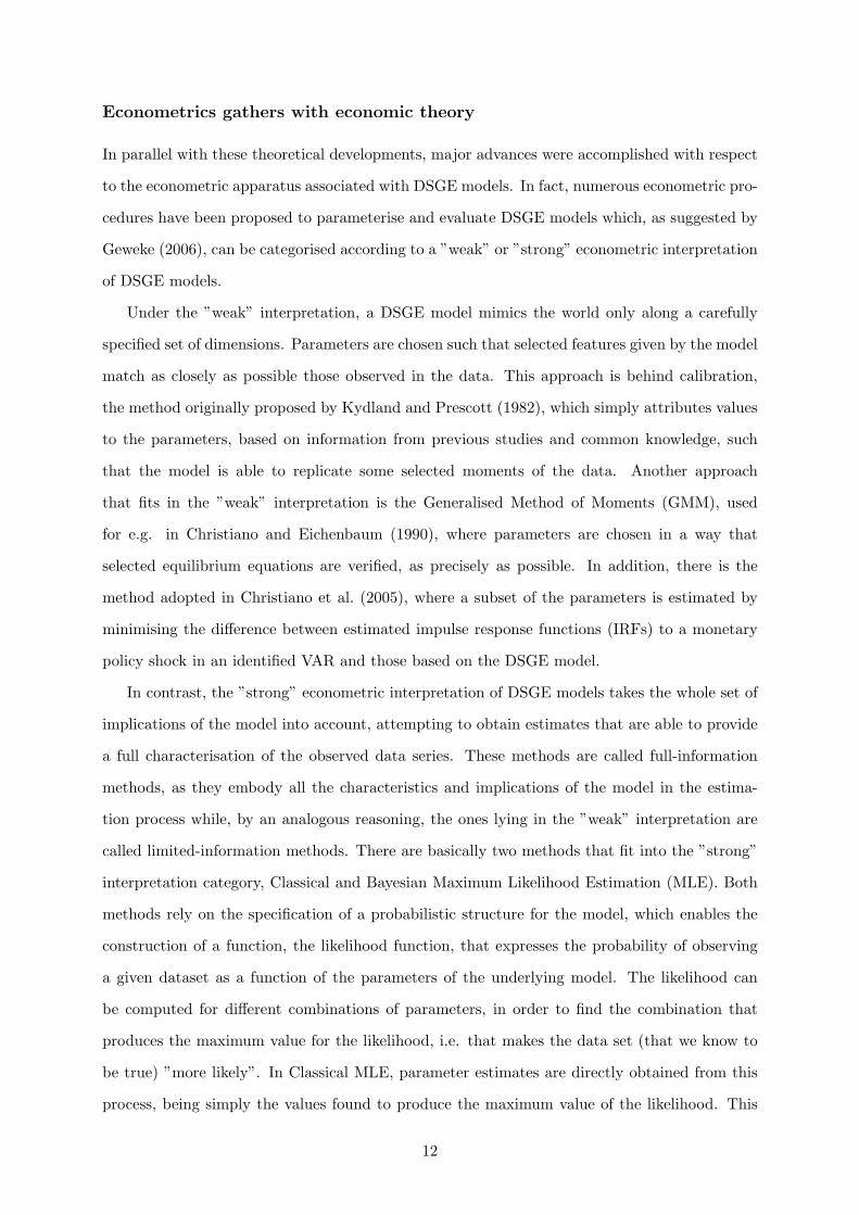
Econometrics gathers with economic theory
In parallel with these theoretical developments, major advances were accomplished with respect
to the econometric apparatus associated with DSGE models. In fact, numerous econometric pro-
cedures have been proposed to parameterise and evaluate DSGE models which, as suggested by
Geweke (2006), can be categorised according to a ”weak” or ”strong” econometric interpretation
of DSGE models.
Under the ”weak” interpretation, a DSGE model mimics the world only along a carefully
specified set of dimensions. Parameters are chosen such that selected features given by the model
match as closely as possible those observed in the data. This approach is behind calibration,
the method originally proposed by Kydland and Prescott (1982), which simply attributes values
to the parameters, based on information from previous studies and common knowledge, such
that the model is able to replicate some selected moments of the data. Another approach
that fits in the ”weak” interpretation is the Generalised Method of Moments (GMM), used
for e.g. in Christiano and Eichenbaum (1990), where parameters are chosen in a way that
selected equilibrium equations are verified, as precisely as possible. In addition, there is the
method adopted in Christiano et al. (2005), where a subset of the parameters is estimated by
minimising the difference between estimated impulse response functions (IRFs) to a monetary
policy shock in an identified VAR and those based on the DSGE model.
In contrast, the ”strong” econometric interpretation of DSGE models takes the whole set of
implications of the model into account, attempting to obtain estimates that are able to provide
a full characterisation of the observed data series. These methods are called full-information
methods, as they embody all the characteristics and implications of the model in the estima-
tion process while, by an analogous reasoning, the ones lying in the ”weak” interpretation are
called limited-information methods. There are basically two methods that fit into the ”strong”
interpretation category, Classical and Bayesian Maximum Likelihood Estimation (MLE). Both
methods rely on the specification of a probabilistic structure for the model, which enables the
construction of a function, the likelihood function, that expresses the probability of observing
a given dataset as a function of the parameters of the underlying model. The likelihood can
be computed for different combinations of parameters, in order to find the combination that
produces the maximum value for the likelihood, i.e. that makes the data set (that we know to
be true) ”more likely”. In Classical MLE, parameter estimates are directly obtained from this
process, being simply the values found to produce the maximum value of the likelihood. This
12

method has been applied by a number of authors to estimate the parameters of DSGE models,
such as Kim (2000) and Ireland (2001). In Bayesian MLE, an additional function is considered,
the prior, representing the a-priori probability that the researcher attributes to different possible
values of the parameters, before observing the data, based on previous studies or on his per-
sonal beliefs. The information from the prior is then combined with the information from the
likelihood and the resulting function can then be maximised, with respect to the parameters,
in a similar way as previously described, until the combination of parameters estimates that
produces the highest value for the objective function is found, i.e. the combination that makes
both the data set and the imposed a-priori beliefs to be ”more likely”. The application of these
techniques to the estimation of a DSGE model was firstly done by DeJong et al. (2000) and
has since then been adopted by several researchers as is the case of Smets and Wouters (2003),
Adolfson et al. (2005), Rabanal and Rubio-Ramırez (2005), Adolfson, Laseen, Linde and Villani
(2007), and Christoffel, Coenen and Warne (2008).
Bayesian techniques stand out
When comparing the two econometric interpretations of a DSGE model, although both have
advantages and disadvantages, the superiority of the ”strong” interpretation is clear, both from
an economic and statistical point of view. On the economic side, it is appealing since parameters
estimates are obtained employing all the restrictions implied by the model, allowing for a more
consistent characterisation of the data generation process. On the statistical side, efficiency is
enhanced by the use of all available information. Furthermore, while the computational burden
associated with full-information methods may have been a problem in the past, computational
methods have dramatically improved over the last years, so that even large-scale models can be
solved quite efficiently.
Within the two full-information methods we have referred, Bayesian estimation is clearly
the one that has gathered more supporters. Classical MLE has proven to be feasible only for
systems of relatively small size and not for the large-scale models that have been used recently.
The main issue has to do with identification problems. In the words of Canova (2007a) ”One
crucial but often neglected condition needed for any methodology to deliver sensible estimates
and meaningful inference is the one of identifiability: the objective function must have a unique
minimum and should display ”enough” curvature in all relevant dimensions”. In models with
a large amount of parameters to estimate it is hard to obtain correct information about all the
13
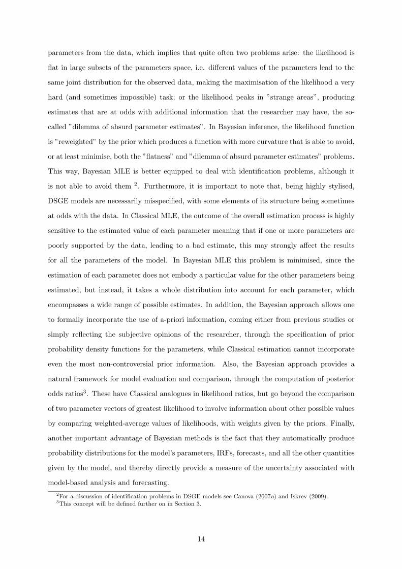
parameters from the data, which implies that quite often two problems arise: the likelihood is
flat in large subsets of the parameters space, i.e. different values of the parameters lead to the
same joint distribution for the observed data, making the maximisation of the likelihood a very
hard (and sometimes impossible) task; or the likelihood peaks in ”strange areas”, producing
estimates that are at odds with additional information that the researcher may have, the so-
called ”dilemma of absurd parameter estimates”. In Bayesian inference, the likelihood function
is ”reweighted” by the prior which produces a function with more curvature that is able to avoid,
or at least minimise, both the ”flatness” and ”dilemma of absurd parameter estimates” problems.
This way, Bayesian MLE is better equipped to deal with identification problems, although it
is not able to avoid them 2. Furthermore, it is important to note that, being highly stylised,
DSGE models are necessarily misspecified, with some elements of its structure being sometimes
at odds with the data. In Classical MLE, the outcome of the overall estimation process is highly
sensitive to the estimated value of each parameter meaning that if one or more parameters are
poorly supported by the data, leading to a bad estimate, this may strongly affect the results
for all the parameters of the model. In Bayesian MLE this problem is minimised, since the
estimation of each parameter does not embody a particular value for the other parameters being
estimated, but instead, it takes a whole distribution into account for each parameter, which
encompasses a wide range of possible estimates. In addition, the Bayesian approach allows one
to formally incorporate the use of a-priori information, coming either from previous studies or
simply reflecting the subjective opinions of the researcher, through the specification of prior
probability density functions for the parameters, while Classical estimation cannot incorporate
even the most non-controversial prior information. Also, the Bayesian approach provides a
natural framework for model evaluation and comparison, through the computation of posterior
odds ratios3. These have Classical analogues in likelihood ratios, but go beyond the comparison
of two parameter vectors of greatest likelihood to involve information about other possible values
by comparing weighted-average values of likelihoods, with weights given by the priors. Finally,
another important advantage of Bayesian methods is the fact that they automatically produce
probability distributions for the model’s parameters, IRFs, forecasts, and all the other quantities
given by the model, and thereby directly provide a measure of the uncertainty associated with
model-based analysis and forecasting.2For a discussion of identification problems in DSGE models see Canova (2007a) and Iskrev (2009).3This concept will be defined further on in Section 3.
14
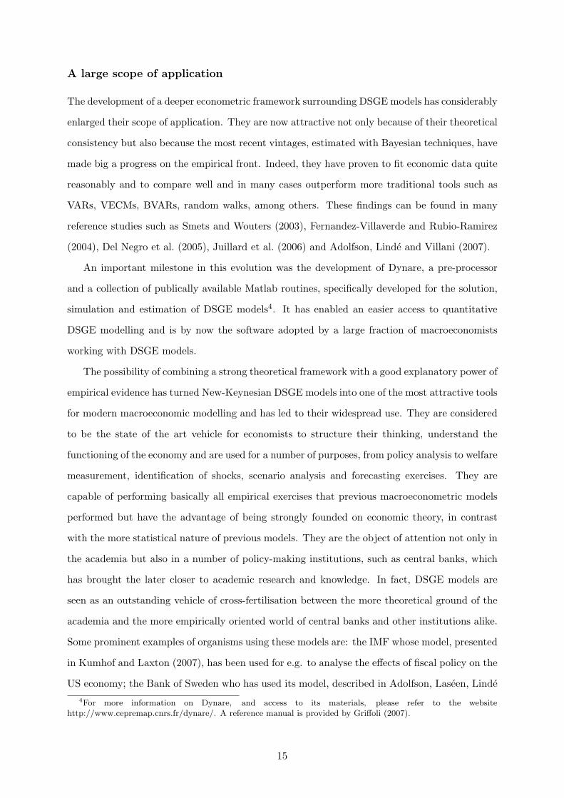
A large scope of application
The development of a deeper econometric framework surrounding DSGE models has considerably
enlarged their scope of application. They are now attractive not only because of their theoretical
consistency but also because the most recent vintages, estimated with Bayesian techniques, have
made big a progress on the empirical front. Indeed, they have proven to fit economic data quite
reasonably and to compare well and in many cases outperform more traditional tools such as
VARs, VECMs, BVARs, random walks, among others. These findings can be found in many
reference studies such as Smets and Wouters (2003), Fernandez-Villaverde and Rubio-Ramirez
(2004), Del Negro et al. (2005), Juillard et al. (2006) and Adolfson, Linde and Villani (2007).
An important milestone in this evolution was the development of Dynare, a pre-processor
and a collection of publically available Matlab routines, specifically developed for the solution,
simulation and estimation of DSGE models4. It has enabled an easier access to quantitative
DSGE modelling and is by now the software adopted by a large fraction of macroeconomists
working with DSGE models.
The possibility of combining a strong theoretical framework with a good explanatory power of
empirical evidence has turned New-Keynesian DSGE models into one of the most attractive tools
for modern macroeconomic modelling and has led to their widespread use. They are considered
to be the state of the art vehicle for economists to structure their thinking, understand the
functioning of the economy and are used for a number of purposes, from policy analysis to welfare
measurement, identification of shocks, scenario analysis and forecasting exercises. They are
capable of performing basically all empirical exercises that previous macroeconometric models
performed but have the advantage of being strongly founded on economic theory, in contrast
with the more statistical nature of previous models. They are the object of attention not only in
the academia but also in a number of policy-making institutions, such as central banks, which
has brought the later closer to academic research and knowledge. In fact, DSGE models are
seen as an outstanding vehicle of cross-fertilisation between the more theoretical ground of the
academia and the more empirically oriented world of central banks and other institutions alike.
Some prominent examples of organisms using these models are: the IMF whose model, presented
in Kumhof and Laxton (2007), has been used for e.g. to analyse the effects of fiscal policy on the
US economy; the Bank of Sweden who has used its model, described in Adolfson, Laseen, Linde4For more information on Dynare, and access to its materials, please refer to the website
http://www.cepremap.cnrs.fr/dynare/. A reference manual is provided by Griffoli (2007).
15

and Villani (2007), both for policy analysis and forecasting; the Bank of Finland with the AINO
model, that can be seen in Kilponen and Ripatti (2006), which besides being applied to the
study of many relevant issues of the Finnish economy, like ageing and demographics, is already
the official forecasting model of Finland’s central bank; and the ECB with the New Area Wide
Model, exposed in Christoffel et al. (2008), which is being used for a wide range of purposes.
For what has been exposed, New-Keynesian DSGE models and their estimation is certainly
one of the most interesting and promising fields in modern macroeconometric research, from
which no country should be left out. In the case of Portugal, some exercises have already been
performed using DSGE models, namely: Pereira and Rodrigues (2000), where an analysis of the
impact of a tax reform package is performed, using a calibrated New-Keynesian model; Fagan
et al. (2004), where the macroeconomic effects of structural changes are investigated, using a
calibrated New-Keynesian model; Silvano (2006) where business cycle movements are studied
using an RBC model estimated with GMM; and Almeida et al. (2008), where the effects of
increasing competition in the nontradable goods and labour markets are inspectioned, using a
calibrated large-scale New-Keynesian model. However, to our knowledge, no attempt has yet
been made to estimate a New-Keynesian DSGE model using Portuguese data. We therefore
consider this to be not only a legitimate but also necessary task, which has led to the conduct
of the present study.
3 On the construction, solution and Bayesian estimation of a
DSGE model
We now provide an overview of the main methodological aspects of our work. It is not our
intention to give an extensive description of the ”formal world” of DSGE models but to present
and justify the main choices and procedures inherent to our research, providing a (as much as
possible) comprehensive understanding of what is ”behind the scenes” of our results 5.
3.1 Model construction and solution
The construction of a DSGE model starts with the specification of the characteristics of the
economy one wishes to model, its environment, its agents, their preferences, technologies and
constraints, and of a set of structural shocks to which the economy is subject. The objectives5We focus, in particular, on the methods applied by Dynare since this is the software we have chosen to adopt.
16

of each agent are then presented, usually involving dynamic optimisation problems for private
agents and policy rules for the fiscal and monetary authorities. Solving the problems of the op-
timising agents with the Lagrange multipliers method one obtains a set of first order conditions,
defining those agents’ decision rules. The equations obtained from this process are then subject
to aggregation procedures, to obtain a set of equations describing the behaviour of economic
agents as a whole, i.e. at the macroeconomic level instead of the microeconomic level from which
we departed. Furthermore, a set of market clearing conditions is specified, to ensure that all the
markets in the economy are in equilibrium in each and every period.
Combining the agents’ behavioural equations, policy rules and constraints (at the aggregate
level) with the market clearing conditions and the shock processes one obtains a set of equations
expressing the endogenous variables of the model at each period as a function of its past, present
and expected future path, of the set of parameters quantifying the relations between variables,
and of the structural exogenous innovations hitting the economy in each period. These equations,
defining our DSGE model, are the starting point of a set of operations which in the end allow
for the computation of a stable, unique, solution to the model. Below, we provide a description
of the main steps needed to achieve this.
Stationarising the model
The first step is rendering all the variables in the model stationary, with a well defined steady-
state to which they return after the economy has been hit by one or more temporary shocks. For
a model like ours, which comprises a unit-root technology shock and inflation in the steady-state,
the following transformations are needed: all non-stationary real variables have to be scaled by
the level of technology; all nominal variables have to be scaled by the numeraire of the economy;
the consumption lagrange multiplier has to be multiplied by the technology level.
Some issues should be referred at this point, although they will probably become more evident
after the model has been presented. First, variables are scaled with the technology level and
numeraire price level of the period in which they are decided and therefore, all predetermined
variables such as the capital stock are scaled with the lagged values of technology and/or price.
Second, being assumed to grow in line with productivity (which grows with technology), the
nominal wage rate needs to be scaled by both the price and technology levels. Finally, foreign
real variables are scaled by the foreign technology level, not the domestic one.
17
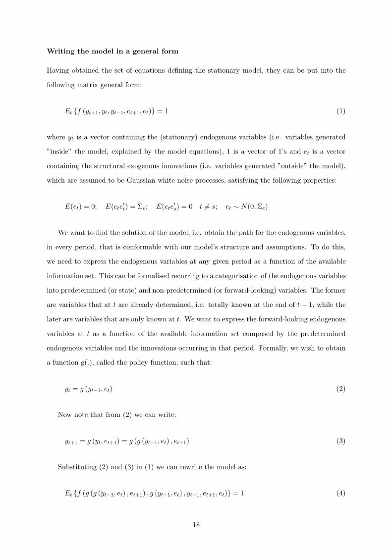
Writing the model in a general form
Having obtained the set of equations defining the stationary model, they can be put into the
following matrix general form:
Et {f (yt+1, yt, yt−1, et+1, et)} = 1 (1)
where yt is a vector containing the (stationary) endogenous variables (i.e. variables generated
”inside” the model, explained by the model equations), 1 is a vector of 1’s and et is a vector
containing the structural exogenous innovations (i.e. variables generated ”outside” the model),
which are assumed to be Gaussian white noise processes, satisfying the following properties:
E(et) = 0; E(ete′t) = Σe; E(ete
′s) = 0 t 6= s; et ∼ N(0, Σe)
We want to find the solution of the model, i.e. obtain the path for the endogenous variables,
in every period, that is conformable with our model’s structure and assumptions. To do this,
we need to express the endogenous variables at any given period as a function of the available
information set. This can be formalised recurring to a categorisation of the endogenous variables
into predetermined (or state) and non-predetermined (or forward-looking) variables. The former
are variables that at t are already determined, i.e. totally known at the end of t− 1, while the
later are variables that are only known at t. We want to express the forward-looking endogenous
variables at t as a function of the available information set composed by the predetermined
endogenous variables and the innovations occurring in that period. Formally, we wish to obtain
a function g(.), called the policy function, such that:
yt = g (yt−1, et) (2)
Now note that from (2) we can write:
yt+1 = g (yt, et+1) = g (g (yt−1, et) , et+1) (3)
Substituting (2) and (3) in (1) we can rewrite the model as:
Et {f (g (g (yt−1, et) , et+1) , g (yt−1, et) , yt−1, et+1, et)} = 1 (4)
18
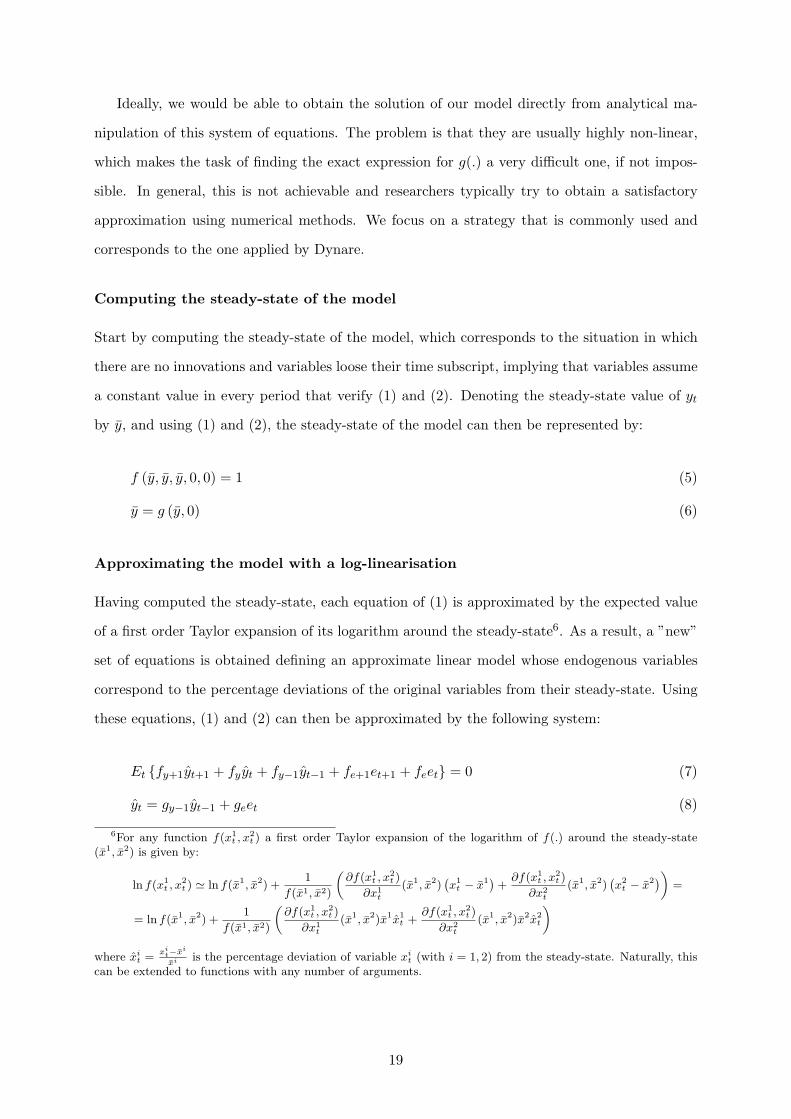
Ideally, we would be able to obtain the solution of our model directly from analytical ma-
nipulation of this system of equations. The problem is that they are usually highly non-linear,
which makes the task of finding the exact expression for g(.) a very difficult one, if not impos-
sible. In general, this is not achievable and researchers typically try to obtain a satisfactory
approximation using numerical methods. We focus on a strategy that is commonly used and
corresponds to the one applied by Dynare.
Computing the steady-state of the model
Start by computing the steady-state of the model, which corresponds to the situation in which
there are no innovations and variables loose their time subscript, implying that variables assume
a constant value in every period that verify (1) and (2). Denoting the steady-state value of yt
by y, and using (1) and (2), the steady-state of the model can then be represented by:
f (y, y, y, 0, 0) = 1 (5)
y = g (y, 0) (6)
Approximating the model with a log-linearisation
Having computed the steady-state, each equation of (1) is approximated by the expected value
of a first order Taylor expansion of its logarithm around the steady-state6. As a result, a ”new”
set of equations is obtained defining an approximate linear model whose endogenous variables
correspond to the percentage deviations of the original variables from their steady-state. Using
these equations, (1) and (2) can then be approximated by the following system:
Et {fy+1yt+1 + fyyt + fy−1yt−1 + fe+1et+1 + feet} = 0 (7)
yt = gy−1yt−1 + geet (8)
6For any function f(x1t , x
2t ) a first order Taylor expansion of the logarithm of f(.) around the steady-state
(x1, x2) is given by:
ln f(x1t , x
2t ) ' ln f(x1, x2) +
1
f(x1, x2)
(∂f(x1
t , x2t )
∂x1t
(x1, x2)(x1
t − x1) +∂f(x1
t , x2t )
∂x2t
(x1, x2)(x2
t − x2))
=
= ln f(x1, x2) +1
f(x1, x2)
(∂f(x1
t , x2t )
∂x1t
(x1, x2)x1x1t +
∂f(x1t , x
2t )
∂x2t
(x1, x2)x2x2t
)
where xit =
xit−xi
xi is the percentage deviation of variable xit (with i = 1, 2) from the steady-state. Naturally, this
can be extended to functions with any number of arguments.
19
where fy+1, fy and fy−1 are the matrix derivatives of f(.) with respect to yt+1, yt and yt−1,
respectively, evaluated in the steady-state; fe+1 and fe are the matrix derivatives of f(.) with
respect to et+1 and et, respectively, evaluated in the steady-state; gy−1 is the derivative of g(.)
with respect to yt−1, evaluated in the steady-state; ge is the derivative of g(.) with respect to et,
evaluated in the steady-state; yt+1, yt and yt−1 are vectors containing the percentage deviations
of the original endogenous variables from their steady-state at times t+1, t and t−1, respectively.
Equation (7) constitutes the general form of the approximate linear model and equation
(8) expresses the corresponding endogenous forward-looking variables as a function of the en-
dogenous state variables and the innovations, which is the analogous of (2) for the approximate
log-linear model. It is characterised by an approximate linear policy function dependent on
matrices gy−1 and ge, which are a function of the deep, structural and policy parameters of
the model, but whose exact composition is yet unknown. gy−1 and ge are called the feedback
and feedforward matrices, respectively. The feedback matrix characterises the impact of the
endogenous state variables on the endogenous forward-looking variables, while the feedforward
matrix characterises the impact of the innovations on the endogenous forward-looking variables.
Once we have obtained the behaviour of the endogenous variables of the approximate linear
model, we can easily recover the values of the original endogenous variables by simply multiplying
their deviations from the steady-state by the corresponding steady-state value and adding this
steady-state value to the obtained result, i.e. for any variable yit:
yit = yi + yiyi
t (9)
Therefore, as long as we can solve the approximate linear model, i.e. obtain gy−1 and ge
that characterise its policy function, given in (8), we will be able to obtain an (approximate)
solution for our original model, by using (9) and the previously computed steady-state. And we
are in fact capable of finding gy−1 and ge by applying some by now well-known techniques for
solving Linear Rational Expectations (LRE) models.
Solving the approximate linear model
To find gy−1 and ge, a series of complex algebraic procedures are needed, which we will present
here in only rough terms, since a detailed explanation is considered to be beyond the scope of
20
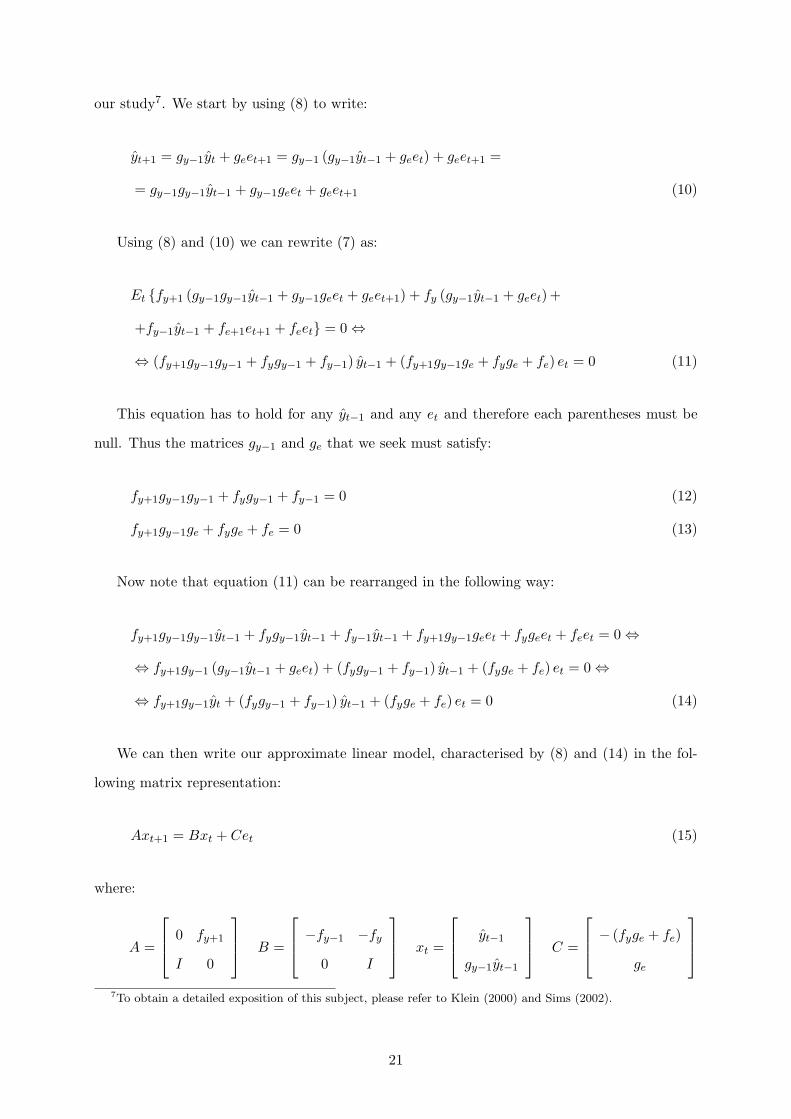
our study7. We start by using (8) to write:
yt+1 = gy−1yt + geet+1 = gy−1 (gy−1yt−1 + geet) + geet+1 =
= gy−1gy−1yt−1 + gy−1geet + geet+1 (10)
Using (8) and (10) we can rewrite (7) as:
Et {fy+1 (gy−1gy−1yt−1 + gy−1geet + geet+1) + fy (gy−1yt−1 + geet)+
+fy−1yt−1 + fe+1et+1 + feet} = 0 ⇔
⇔ (fy+1gy−1gy−1 + fygy−1 + fy−1) yt−1 + (fy+1gy−1ge + fyge + fe) et = 0 (11)
This equation has to hold for any yt−1 and any et and therefore each parentheses must be
null. Thus the matrices gy−1 and ge that we seek must satisfy:
fy+1gy−1gy−1 + fygy−1 + fy−1 = 0 (12)
fy+1gy−1ge + fyge + fe = 0 (13)
Now note that equation (11) can be rearranged in the following way:
fy+1gy−1gy−1yt−1 + fygy−1yt−1 + fy−1yt−1 + fy+1gy−1geet + fygeet + feet = 0 ⇔
⇔ fy+1gy−1 (gy−1yt−1 + geet) + (fygy−1 + fy−1) yt−1 + (fyge + fe) et = 0 ⇔
⇔ fy+1gy−1yt + (fygy−1 + fy−1) yt−1 + (fyge + fe) et = 0 (14)
We can then write our approximate linear model, characterised by (8) and (14) in the fol-
lowing matrix representation:
Axt+1 = Bxt + Cet (15)
where:
A =
0 fy+1
I 0
B =
−fy−1 −fy
0 I
xt =
yt−1
gy−1yt−1
C =
− (fyge + fe)
ge
7To obtain a detailed exposition of this subject, please refer to Klein (2000) and Sims (2002).
21
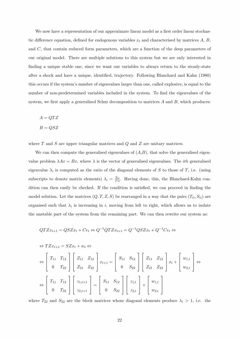
We now have a representation of our approximate linear model as a first order linear stochas-
tic difference equation, defined for endogenous variables xt and characterised by matrices A, B,
and C, that contain reduced form parameters, which are a function of the deep parameters of
our original model. There are multiple solutions to this system but we are only interested in
finding a unique stable one, since we want our variables to always return to the steady-state
after a shock and have a unique, identified, trajectory. Following Blanchard and Kahn (1980)
this occurs if the system’s number of eigenvalues larger than one, called explosive, is equal to the
number of non-predetermined variables included in the system. To find the eigenvalues of the
system, we first apply a generalised Schur decomposition to matrices A and B, which produces:
A = QTZ
B = QSZ
where T and S are upper triangular matrices and Q and Z are unitary matrices.
We can then compute the generalised eigenvalues of (A,B), that solve the generalised eigen-
value problem λAx = Bx, where λ is the vector of generalised eigenvalues. The ith generalised
eigenvalue λi is computed as the ratio of the diagonal elements of S to those of T , i.e. (using
subscripts to denote matrix elements) λi = SiiTii . Having done, this, the Blanchard-Kahn con-
dition can then easily be checked. If the condition is satisfied, we can proceed in finding the
model solution. Let the matrices (Q,T, Z, S) be rearranged in a way that the pairs (Tii, Sii) are
organised such that λi is increasing in i, moving from left to right, which allows us to isolate
the unstable part of the system from the remaining part. We can then rewrite our system as:
QTZxt+1 = QSZxt + Cet ⇔ Q−1QTZxt+1 = Q−1QSZxt + Q−1Cet ⇔
⇔ TZxt+1 = SZxt + wt ⇔
⇔
T11 T12
0 T22
Z11 Z12
Z21 Z22
xt+1 =
S11 S12
0 S22
Z11 Z12
Z21 Z22
xt +
w1,t
w2,t
⇔
⇔
T11 T12
0 T22
z1,t+1
z2,t+1
=
S11 S12
0 S22
z1,t
z2,t
+
w1,t
w2,t
where T22 and S22 are the block matrices whose diagonal elements produce λi > 1, i.e. the
22

matrices containing the unstable part of the system, z2,t = [Z21 Z22] xt and wt = Q−1Cet.
Then, using the lower block of this system, we can write a sub-system containing all the explosive
generalised eigenvalues:
T22z2,t+1 = S22z2,t + w2,t (16)
Solving for z2,t yields:
z2,t = Pz2,t+1 − S−122 w2,t (17)
where P = S−122 T22. Performing recursive substitution for z2,t+1, z2,t+2,..., we obtain:
z2,t = P(Pz2,t+2 − S−1
22 w2,t+1
)− S−122 w2,t =
= P 2z2,t+2 − PS−122 w2,t+1 − S−1
22 w2,t =
= P 2(Pz2,t+3 − S−1
22 w2,t+2
)− PS−122 w2,t+1 − S−1
22 w2,t =
= P 3z2,t+3 − P 2S−122 w2,t+2 − PS−1
22 w2,t+1 − S−122 w2,t =
= P iz2,t+i −∞∑
i=0
P iS−122 w2,t+i (18)
Now note that P−1 = T−122 S22 is a diagonal matrix containing the system’s explosive eigenvalues
and therefore its inverse, P , is also a diagonal matrix containing the inverse of those eigenvalues.
Therefore P t converges to zero as t increases, implying:
P iz2,t+i = 0 (19)
Therefore, z2,t can be written as:
z2,t = −∞∑
i=1
P i−1S−122 w2,t+i (20)
This means that z2,t can be expressed solely as a function of future shocks whose expected
value at t is zero implying:
z2,t = 0 ⇔[
Z21 Z22
]xt = 0 ⇔
[Z21 Z22
]
yt
gy−1yt
= 0 ⇔
23
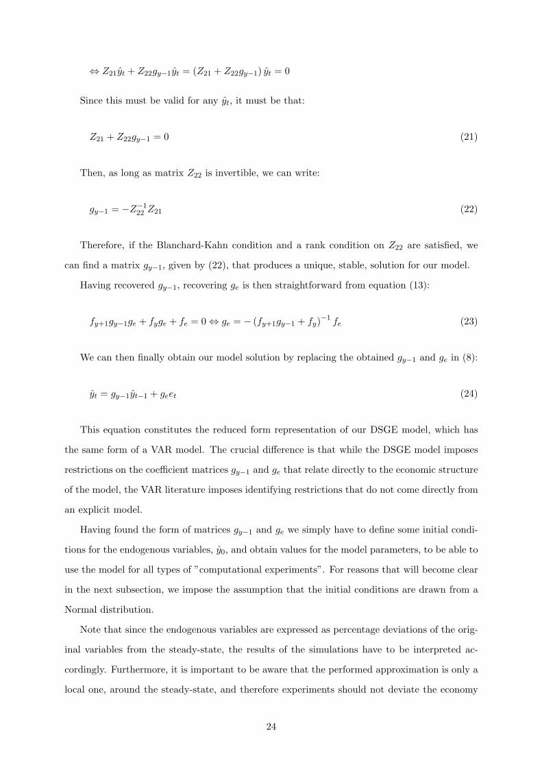
⇔ Z21yt + Z22gy−1yt = (Z21 + Z22gy−1) yt = 0
Since this must be valid for any yt, it must be that:
Z21 + Z22gy−1 = 0 (21)
Then, as long as matrix Z22 is invertible, we can write:
gy−1 = −Z−122 Z21 (22)
Therefore, if the Blanchard-Kahn condition and a rank condition on Z22 are satisfied, we
can find a matrix gy−1, given by (22), that produces a unique, stable, solution for our model.
Having recovered gy−1, recovering ge is then straightforward from equation (13):
fy+1gy−1ge + fyge + fe = 0 ⇔ ge = − (fy+1gy−1 + fy)−1 fe (23)
We can then finally obtain our model solution by replacing the obtained gy−1 and ge in (8):
yt = gy−1yt−1 + geet (24)
This equation constitutes the reduced form representation of our DSGE model, which has
the same form of a VAR model. The crucial difference is that while the DSGE model imposes
restrictions on the coefficient matrices gy−1 and ge that relate directly to the economic structure
of the model, the VAR literature imposes identifying restrictions that do not come directly from
an explicit model.
Having found the form of matrices gy−1 and ge we simply have to define some initial condi-
tions for the endogenous variables, y0, and obtain values for the model parameters, to be able to
use the model for all types of ”computational experiments”. For reasons that will become clear
in the next subsection, we impose the assumption that the initial conditions are drawn from a
Normal distribution.
Note that since the endogenous variables are expressed as percentage deviations of the orig-
inal variables from the steady-state, the results of the simulations have to be interpreted ac-
cordingly. Furthermore, it is important to be aware that the performed approximation is only a
local one, around the steady-state, and therefore experiments should not deviate the economy
24
considerably from the steady-state, since in this case the approximation will no longer be valid.
Our approach to finding parameters estimates relies on the Bayesian MLE methodology and
therefore the next subsections focus on the procedures associated with it.
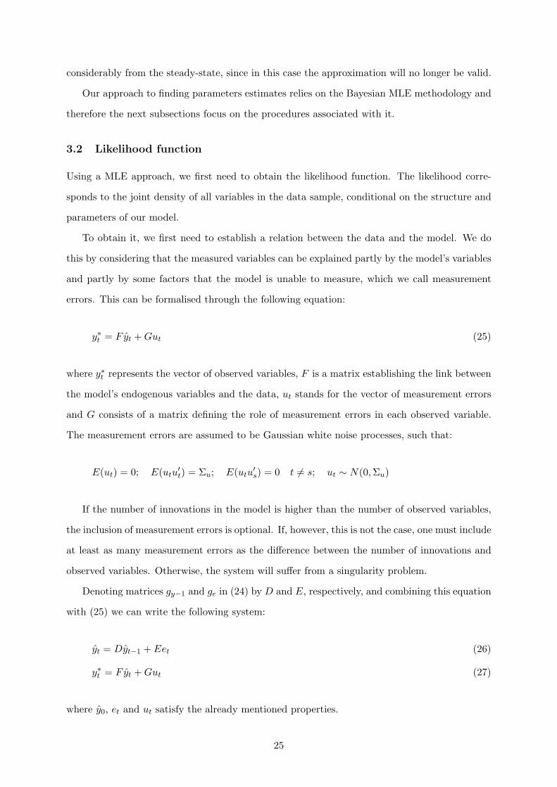
3.2 Likelihood function
Using a MLE approach, we first need to obtain the likelihood function. The likelihood corre-
sponds to the joint density of all variables in the data sample, conditional on the structure and
parameters of our model.
To obtain it, we first need to establish a relation between the data and the model. We do
this by considering that the measured variables can be explained partly by the model’s variables
and partly by some factors that the model is unable to measure, which we call measurement
errors. This can be formalised through the following equation:
y∗t = F yt + Gut (25)
where y∗t represents the vector of observed variables, F is a matrix establishing the link between
the model’s endogenous variables and the data, ut stands for the vector of measurement errors
and G consists of a matrix defining the role of measurement errors in each observed variable.
The measurement errors are assumed to be Gaussian white noise processes, such that:
E(ut) = 0; E(utu′t) = Σu; E(utu
′s) = 0 t 6= s; ut ∼ N(0,Σu)
If the number of innovations in the model is higher than the number of observed variables,
the inclusion of measurement errors is optional. If, however, this is not the case, one must include
at least as many measurement errors as the difference between the number of innovations and
observed variables. Otherwise, the system will suffer from a singularity problem.
Denoting matrices gy−1 and ge in (24) by D and E, respectively, and combining this equation
with (25) we can write the following system:
yt = Dyt−1 + Eet (26)
y∗t = F yt + Gut (27)
where y0, et and ut satisfy the already mentioned properties.
25
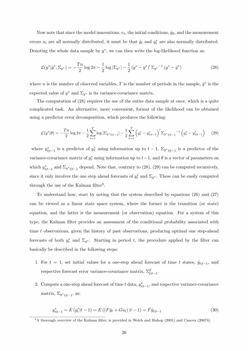
Now note that since the model innovations, et, the initial conditions, y0, and the measurement
errors ut are all normally distributed, it must be that yt and y∗t are also normally distributed.
Denoting the whole data sample by y∗, we can then write the log-likelihood function as:
L(y∗|y∗, Σy∗) = −Tn
2log 2π − 1
2log |Σy∗ | − 1
2(y∗ − y∗)′Σy∗
−1 (y∗ − y∗) (28)
where n is the number of observed variables, T is the number of periods in the sample, y∗ is the
expected value of y∗ and Σy∗ is its variance-covariance matrix.
The computation of (28) requires the use of the entire data sample at once, which is a quite
complicated task. An alternative, more convenient, format of the likelihood can be obtained
using a predictor error decomposition, which produces the following:
L(y∗|θ) = −Tn
2log 2π − 1
2
T∑t=1
log |Σy∗ t|t−1| −12
T∑t=1
(y∗t − y∗t|t−1
)′Σy∗ t|t−1
−1(y∗t − y∗t|t−1
)(29)
where y∗t|t−1 is a predictor of y∗t using information up to t − 1, Σy∗ t|t−1 is a predictor of the
variance-covariance matrix of y∗t using information up to t−1, and θ is a vector of parameters on
which y∗t|t−1 and Σy∗ t|t−1 depend. Note that, contrary to (28), (29) can be computed recursively,
since it only involves the one step ahead forecasts of y∗t and Σy∗ . These can be easily computed
through the use of the Kalman filter8.
To understand how, start by noting that the system described by equations (26) and (27)
can be viewed as a linear state space system, where the former is the transition (or state)
equation, and the latter is the measurement (or observation) equation. For a system of this
type, the Kalman filter provides an assessment of the conditional probability associated with
time t observations, given the history of past observations, producing optimal one step-ahead
forecasts of both y∗t and Σy∗ . Starting in period t, the procedure applied by the filter can
basically be described in the following steps:
1. For t = 1, set initial values for a one-step ahead forecast of time t states, yt|t−1, and
respective forecast error variance-covariance matrix, Σyt|t−1.
2. Compute a one-step ahead forecast of time t data, y∗t|t−1, and respective variance-covariance
matrix, Σy∗ t|t−1, as:
y∗t|t−1 = E (y∗t |t− 1) = E ((F yt + Gut) |t− 1) = F yt|t−1 (30)
8A thorough overview of the Kalman filter, is provided in Welch and Bishop (2001) and Canova (2007b).
26
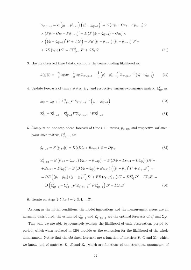
Σy∗ t|t−1 = E(y∗t − y∗t|t−1
)(y∗t − y∗t|t−1
)′= E
(F yt + Gut − F yt|t−1
)×
× (F yt + Gut − F yt|t−1
)′ = E(F
(yt − yt|t−1
)+ Gut
)×
×((
yt − yt|t−1
)′F ′ + u′tG
′)
= FE(yt − yt|t−1
) (yt − yt|t−1
)′F ′+
+ GE(utu
′t
)G′ = FΣy
t|t−1F′ + GΣuG′ (31)
3. Having observed time t data, compute the corresponding likelihood as:
L(y∗t |θ) = −n
2log 2π − 1
2log |Σy∗ t|t−1| −
12
(y∗t − y∗t|t−1
)′Σy∗ t|t−1
−1(y∗t − y∗t|t−1
)(32)
4. Update forecasts of time t states, yt|t, and respective variance-covariance matrix, Σyt|t, as:
yt|t = yt|t−1 + Σyt|t−1F
′Σy∗ t|t−1−1
(y∗t − y∗t|t−1
)(33)
Σyt|t = Σy
t|t−1 − Σyt|t−1F
′Σy∗ t|t−1−1FΣy
t|t−1 (34)
5. Compute an one-step ahead forecast of time t + 1 states, yt+1|t, and respective variance-
covariance matrix, Σyt+1|t, as:
yt+1|t = E (yt+1|t) = E ((Dyt + Eet+1) |t) = Dyt|t (35)
Σyt+1|t = E
(yt+1 − yt+1|t
) (yt+1 − yt+1|t
)′ = E(Dyt + Eet+1 −Dyt|t
)(Dyt+
+Eet+1 −Dyt|t)′ = E
(D
(yt − yt|t
)+ Eet+1
) ((yt − yt|t
)′D′ + e′t+1E
′)
=
= DE((
yt − yt|t) (
yt − yt|t)′)
D′ + EE(et+1e
′t+1
)E′ = DΣy
t|tD′ + EΣeE
′ =
= D(Σy
t|t−1 − Σyt|t−1F
′Σy∗ t|t−1−1FΣy
t|t−1
)D′ + EΣeE
′ (36)
6. Iterate on steps 2-5 for t = 2, 3, 4, ..., T .
As long as the initial conditions, the model innovations and the measurement errors are all
normally distributed, the estimated y∗t|t−1 and Σy∗ t|t−1 are the optimal forecasts of y∗t and Σy∗ .
This way, we are able to recursively express the likelihood of each observation, period by
period, which when replaced in (29) provide us the expression for the likelihood of the whole
data sample. Notice that the obtained forecasts are a function of matrices F , G and Σu, which
we know, and of matrices D, E and Σe, which are functions of the structural parameters of
27

our original model, that we intend to estimate. Therefore, the likelihood function we obtain is
simply a function of the original model’s parameters, which is exactly what we intended.
3.3 Prior distributions
The next step is the specification of prior distributions for the parameters we want to estimate,
p(θ), which is where the Bayesian component of the estimation process starts. Each prior is a
probability density function of a parameter, constituting a formal way of specifying probabilities
to each value that the parameter can assume, based on past studies or/and occurrences or simply
reflecting subjective views of the researcher. Either way, it is basically a representation of belief
in the context of the model under analysis, being constructed without any reference to the
data set contained in the estimation sample constituting an additional, independent, source of
information on the model’s parameters.
The specification of a prior starts with the selection of the most adequate functional form for
the distribution. This can be done on the basis of a number of criteria, with some of the most
common ones being: inverse gamma distribution for parameters bounded to be positive; beta
distribution for parameters bounded between zero and one; normal distribution for parameters
that are not bounded.
It is then necessary to choose values for the parameters defining each of the distributions,
which are usually measures of location (e.g. mode and mean) and dispersion (e.g. standard de-
viation and probability intervals). For this, parameters are usually grouped into two categories:
parameters for which we have relatively strong a priori convictions, which comprises the model’s
core structural parameters; and parameters for which we are quite uncertain about, which in-
cludes the parameters that characterise the stochastic shocks. Priors for the parameters in the
first category are based on our reading of existing empirical evidence and their implications for
macroeconomic dynamics. For parameters in the second category, although we can also recur to
existing studies, the strategy is mainly to set priors with reasonable means and a density with
a large support so that the distribution can cover a considerable range of parameter values, i.e.,
priors that are only weakly informative.
Since the prior is generated from well-known densities, its computation is straightforward.
28
3.4 Posterior distributions
Having derived the likelihood and specified the priors, we can then estimate the posterior distri-
bution. The posterior represents the probabilities assigned to different values of the parameters
after observing the data. It basically constitutes an update of the probabilities given by the
prior, based on the additional information provided by the variables in our sample. To express
formally how the posterior relates to the likelihood and the priors we apply the well-known
Bayes theorem to the two random events θ and y∗, which produces:
p (θ|y∗) =p (θ, y∗)p (y∗)
(37)
p (y∗|θ) =p (θ, y∗)
p (θ)⇔ p (θ, y∗) = p (y∗|θ) p (θ) (38)
where p (θ|y∗) is the density of the parameters conditional on the data (the posterior), p (θ, y∗)
is the joint density of the parameters and the data, p (y∗|θ) is the density of the data conditional
on the parameters (the likelihood), p (θ) is the unconditional density of the parameters (the
prior) and p (y∗) is the marginal density of the data (this concept will be further explored in the
next subsection). Replacing (38) in (37):
p (θ|y∗) =p (y∗|θ) p (θ)
p (y∗)(39)
Now note that p (y∗) does not depend on the parameters and therefore, in what concerns
the estimation of the parameters, can be treated as a constant, enabling us to write:
p (θ|y∗) ∝ p (y∗|θ) p (θ) = K (θ|y∗) (40)
where K (θ|y∗) is the posterior kernel, which is proportional to the posterior by the factor p (y∗).
Taking logs:
lnK (θ|y∗) = ln p (y∗|θ) + ln p (θ) = L(y∗|θ) + ln p (θ) (41)
Assuming that priors are independently distributed, this equation may be calculated as:
lnK (θ|y∗) = L(y∗|θ) +∑ג
x=1
ln p (θx) (42)
29

where ג is the number of parameters being estimated. This is the equation that will allow us to
estimate the posteriors. It is however analytically intractable, since it is a nonlinear complicated
function of the parameters contained in θ, and therefore the analysis has to be performed with
numerical methods.
We start by maximizing (42) with respect to θ to obtain an estimate for the mode of the
posterior distribution, θm, and for the Hessian matrix evaluated at the mode, H(θm) (note that
the maximum of p (θ|y∗) will be the same as the maximum of K (θ|y∗)). This is carried out using
an optimisation routine (csmiwell) developed by Christopher Sims.
We then use a Monte-Carlo Markov-Chain (MCMC) sampling method, specifically the
Metropolis-Hastings (MH) algorithm, to simulate the posterior distributions. The general idea
of the algorithm is to generate a Markov-Chain that represents a sequence of possible parameter
estimates, in a way that the whole domain of the parameter space is explored, and then use the
frequencies associated with each estimate to build an histogram that mimics the posterior dis-
tribution. To do so, the algorithm starts by specifying a ”candidate” (or jumping) distribution,
from which several parameter estimates are drawn and then poses an ”acceptance-rejection”
rule according to which some of the generated estimates are kept and some are not. To pick
the ”candidate” distribution, the algorithm builds on the fact that under fairly general regu-
larity conditions, the posterior will be asymptotically normal, and uses the mode and Hessian
obtained from the maximisation of the posterior kernel to define the mean and variance. The
variance is built as the inverse of the Hessian multiplied by a constant, called the scale factor,
which is a crucial parameter, since it determines the acceptance ratio, i.e. the percentage of
estimates generated from the jumping distribution that are kept to construct the posterior. In
the words of An and Schorfheide (2007), the algorithm ”constructs a Gaussian approximation
around the posterior mode and uses a scaled version of the asymptotic covariance matrix as
the covariance matrix for the proposal distribution. This allows for an efficient exploration of
the posterior distribution at least in the neighborhood of the mode”. More precisely, the MH
algorithm implements the following steps:
1. Consider a jumping distribution for the model’s parameters given by:
J(θ∗|θt−1
)= N
(θt−1, cΣθm
)(43)
where θt−1 is the distributions’s jumping mean, whose initial value is set to the previously
30
estimated posterior mode, Σθm is the variance of the distribution, computed as the inverse
of the previously estimated Hessian matrix, and c is a scale factor.
2. Draw a proposal new estimate θ∗ from the distribution.
3. Compute r, the ratio of the posterior kernel evaluated at the new proposal estimate over
the posterior kernel evaluated at the previous proposal estimate:
r =K (θ∗|y∗)K (θt−1|y∗) (44)
4. Accept or discard θ∗ as the new estimate according to the following rule:
θt =
θ∗ with probability min(r,1)
θt−1 otherwise
5. If θ∗ is accepted update the mean of the distribution, otherwise keep the previous one.
6. Loop on steps 2-5.
7. Having done enough loops, use the accepted draws to built an histogram.
It is important to understand the intuition behind this mechanism. When r > 1 we will
definitely keep θ∗ since it produces a higher value for the posterior than θt−1, i.e., given our
sample, it is more likely to have θ∗ than θt−1. When 0 ≤ r ≤ 1, the proposal estimate produces
a lower value for the posterior. However, we will not discard this estimate immediately, we will
accept it with probability r and reject it with probability 1− r. The point is that to be able to
visit the entire domain of the posterior distribution, we should not be too quick to simply throw
out the candidate giving a lower value of the posterior kernel, because it might be the case that
the candidate allows us to leave a local maximum and travel towards the global maximum. As
clearly said in Griffoli (2007) ”the idea is to allow the search to turn away from taking a small
step up and instead take a few small steps down in the hope of being able to take a big step up
in the near future”. This will produce a sample of diversified parameter estimates, where highly
likely values are represented by multiple occurrences, forming the center of the distribution, but
less likely values are also considered, forming the tails of the distribution.
A fundamental part of this procedure is the variance of the jumping distribution and in
particular the scale factor. If the variance is too small, the acceptance rate, i.e. the fraction of
31
draws that are accepted, will be too high and the Markov chain will not be able to do a good
job in visiting the entire distribution, and will probably get ”stuck” around a local maximum.
However, if the variance is too high, the acceptance rate will be too small and the chain will
spend much time visiting the tails of the distribution and will have difficulty in finding the
maximum. Therefore, c will be crucial to ”fine-tune” the variance of the jumping distribution,
such that the acceptance rate is neither too big nor to small. Another important aspect is the
number of iterations performed by the algorithm. The bigger the number, the smoother will be
the histogram, since each ”bucket” of the histogram will have less and less weight in the overall
distribution, and the closer will be the histogram to the desired theoretical distribution.
This way, we are able to obtain an approximation of the posterior distributions, characterised
by the usual measures of location (mode, mean) and dispersion (standard deviation, percentiles),
which provide not only point estimates of the parameters of the model but also a measure of
the uncertainty surrounding those estimates.
Beyond the calculation of posterior moments and distributions themselves, one can use these
results for a number of applications, which explore the model’s theoretical and empirical impli-
cations in an informative way. Some of the most common and relevant ones are: forecasting,
where departing from an initial state the future behaviour of the endogenous variables is pre-
dicted; historical decomposition, where the historical evolution of the observed variables, used
in the estimation, can be decomposed into the contributions of the structural shocks considered
in the model and the lagged effect of the initial state, allowing one to conclude on the main
driving forces behind the economy’s behaviour; IRFs, which corresponded to estimates of the
effect of each shock on the endogenous variables; forecast-error-variance decompositions, which
decompose the variance of the error in forecasting the endogenous variables into the contribu-
tions of the variance of each shock; counterfactual scenarios, where the consequences of assuming
a difference in some feature of the model are explored. For all these applications, we can obtain
not only point estimates, but also confidence intervals, by simply using the draws produced by
the MH algorithm.
3.5 Evaluation of the estimation results
A crucial part of the process of estimating a model is the conduction of an evaluation of its
results. In the case of a DSGE model, estimated with a Bayesian approach, this can be done
in a number of ways, using both techniques that are common to other estimation methods and
32

techniques that are exclusively used in a Bayesian context. We consider three broad classes of
aspects that can be inspectioned in order to assess the quality of the estimated model: validation
of the estimation procedures and results, ability of the model to fit the data’s characteristics
and comparison with alternative models.
Checking the estimation diagnosis and results
The first thing to check is the quality of the posterior kernel numerical maximisation. We do
this by plotting the minus of the posterior kernel for values around the computed mode, for each
estimated parameter in turn. If the estimated mode is not at the trough (bottom minus) of the
distribution, there is a clear sign that the numerical procedure is having a hard time finding the
optimum. This can be related to poor priors or to identification problems.
Secondly, if one concludes that the numerical procedure is working well, then the parameters
mode and standard deviation estimates can be inspectioned. They should be plausible both
from a statistical and an economic point of view. For this, comparison with previous studies
and evidence from micro data can be of extreme usefulness.
Thirdly, if the estimates seem to be reasonable, they can be considered as good initial values
for the MH algorithm and, therefore, we can proceed by examining its convergence properties.
This is the main source of feedback to gain confidence or spot a problem with the results. To
obtain it, one should conduct several distinct runs of MH simulations, with each one starting
at a different initial value, and for each run perform a large number of draws. If convergence
is achieved, and the optimiser did not get stuck in an odd area of the parameter subspace, two
things should happen: results within each run’s iterations should be similar; results between
different runs should be close. When convergence is not achieved, the problem is usually related
to poor priors or to an insufficient number of MH iterations.
Fourthly, it is necessary to inspect the simulated posterior distribution and confront it with
both the prior distribution and the posterior mode obtained by the maximisation of the posterior
kernel. First, the posterior distributions should be approximately normal. Second, the prior
and posterior should not be excessively different nor excessively similar. If they are very far
from each other, this may indicate that the priors are imposing erroneous restrictions on the
data. If they are too similar, results are probably being mostly led by the prior and only
marginally by the data. In fact, informative posterior distributions can be obtained even when
the parameters are not identified in the data, if a tight enough prior distribution is specified. The
33

posteriors will appear to be well behaved only because the prior has selected a particular region
of the parameter space. While the prior should be used to exclude regions of the parameter
space that are unreasonable from an economic point of view, it should also be made reasonably
uninformative on the interesting portions of the parameters space to let the data speak and avoid
misleading conclusions. The shift from the prior to the posterior can be seen as an indicator of
the tension between the two sources of information, prior and data. If, for a given parameter, the
two distributions are virtually the same, one can conclude that the estimation results concerning
that parameter are being mostly determined by the prior and that either the data is silent on
that parameter or we are simply not allowing the data to speak. In this case, altering both the
shape and the dispersion of the prior may help to detect identification problems and provide a
clearer notion of which estimates are strongly supported by the data and which are not. Third,
the mode of the simulated posterior distribution should note be too far from the mode calculated
from the numerical optimisation of the posterior kernel.
Fifthly, the estimates of the structural shocks should be inspectioned to eye-ball the plausibil-
ity of the size and frequency of the innovations. In particular, these should exhibit a stationary,
i.i.d, behaviour and be centered around zero.
Finally, one can perform a sensitivity analysis, by making changes in the assumptions con-
cerning the priors or even using a different data set. Note, however, that this can be a tricky
task, especially when the data is not well behaved.
Assessing the absolute fit of the model
Having checked the robustness and reasonability of the estimation results, what any empirical
researcher wishes to see is the ability of the estimated model to match the empirical properties
of the data. One way of inspecting this is to compare a set of relevant statistics computed with
the actual data to the same set of statistics computed with data simulated by the model. These
are usually the sample moments, in particular the mean and variance.
Furthermore, the Kalman filter estimates of the observed variables, computed at θm and
Σθm can be given the same interpretation as the fitted values of a regression, and can therefore
be loosely interpreted as the in-sample fit of the model.
34

Assessing the relative fit of the model
Besides the assessment of the model’s absolute fit, it is also interesting and meaningful to study
its relative fit, i.e., how it compares to the fit of other, alternative, models. This can be done for
different specifications of the DSGE model, giving an indication of the role of different possible
model extensions. However, it may very well be that all of the DSGE models are severely
misspecified, as the cross-coefficient restrictions they impose may be too strong. Therefore, it
is also useful to compare the model with more flexible and empirically oriented models, like
VARs, BVARs and random walks, as long as they are estimated on the same data set. This
way, one can understand the degree of misspecification of the DSGE model and relax some of
its restrictions so that, while still maintaining a strong economic foundation the model, it is also
able to do a good job on the empirical ground.
The crucial tool needed to perform model comparison in a Bayesian framework is the marginal
likelihood function, p (y∗|i). It corresponds to the density of the data, conditional on the model
but unconditional on the model’s parameters, constituting a measure of the likelihood attributed
by the model to the data that was in fact observed. It is obtained by integrating out the
parameters from the joint density of the data and the parameters which, recalling the expression
given in (38), is equivalent to the integral of the posterior kernel over the parameter space.
Formally, for a given model i, we this amounts to:
p (y∗|i) =∫
θi
p (y∗, θi|i) dθi =∫
θi
p (y∗|θi, i) p (θi|i) dθi =∫
θi
K (θi|y∗, i) dθi (45)
where p (θi|i), p (y∗|θi, i) and K (θi|y∗, i) are simply the usual prior, likelihood and posterior
kernel, stated explicitly as a function of the specific model under analysis9.
This expression involves multidimensional integration, which is analytically intractable, and
therefore it is necessary to recur to numerical approximations. The two most common approaches
are the Laplace approximation and the Harmonic mean estimator. The first approach assumes
that the posterior kernel can be approximated by a Gaussian distribution, and evaluates its
integral at the mode and variance obtained with the numerical maximisation of the posterior
kernel. This produces the following estimator for the marginal likelihood:
p (y∗|i)L = 2πn2 |Σθm
i| 12 p(θm
i |y∗, i)p(θmi |i) (46)
9This was not made explicit before for notational simplicity.
35
The second approach uses the MH runs to simulate the marginal likelihood and then simply
takes the average of these simulated values. It makes use of the fact that:
p (y∗|i) = E
[f (θi)
K (θi|y∗, i) |θi
]−1
=
[ ∫θi
f (θi) dθi∫θiK (θi|y∗, i) dθi
]−1
(47)
where f (θi) is a probability density function such that∫θi
f (θi) dθi = 1. This suggests the
following estimator for the marginal likelihood:
p (y∗|i)MH =
1
B
B∑
b=1
f(θ(b)i
)
K(θ(b)i |y∗, i
)−1
(48)
where θ(b)i represents each drawn vector from the MH iterations, B is the total number of
iterations and f(θ(b)i
)can be viewed as a weighting factor on the posterior kernel in order to
downplay the importance of extreme values of θi.
The advantage of the first technique is its computational efficiency: time consuming Metropolis-
Hastings iterations are not necessary, only the numerically calculated posterior mode and Hessian
matrix are required. However, the second method is preferable, since it does not impose any
functional form on the posterior kernel which, if incorrect, may lead to erroneous results.
By representing the overall likelihood attributed by the model to the observed data set,
independently of the parameters of the model, the marginal likelihood is naturally a measure
of the model’s unconditional overall fit. Furthermore, it is a measure of the model’s out-of-
sample predictive performance. To see this, it is necessary to introduce the concept of predictive
density, a function that represents the out of sample performance of a given model, for a given
set of variables, whether they have already been observed or are still going to be observed in
the future. Standing at time t, the predictive density for future y’s, until time T , conditional on
model i, is given by:
p(yt+1, ..., yT |Yt, i) =∫
θi
p(yt+1, ..., yT |Yt, i, θi)p(θi|Yt, i)dθi =
=∫
θi
T∏
s=t+1
p(yt|Yt−1, i, θi)p(θi|Yt, i)dθi =T∏
s=t+1
p(yt|Yt−1, i) (49)
where Yt = yt, ..., y1 is the information set available at time t, p(θi|yt, i) is the posterior of
θ, conditional on model i and on the information set until t, and∏T
s=t+1 p(yt|Yt−1, θi, i) is
36

the recursive one-step ahead predictive density constructed from the model. As a function of
yt+1, ..., yT , after observing Yt and before observing yt+1, ..., yT , this expression is the predictive
density of yt+1, ..., yT conditional on Yt and model i. Following the observation of yt+1, ..., yT , it
is a real number, known as the predictive likelihood of yt+1, ..., yT conditional on Yt and model
i. Now note that if we have a sample of T periods and we want to predict all the observations
in the sample we have that Y0 = {∅} and therefore we can write:
p(y1, ..., yT |i) =∫
θi
p(y1, ..., yT |i, θi)p(θi|i)dθi =
=∫
θi
T∏
t=1
p(yt|Yt−1, i, θi)p(θi|i)dθi =T∏
t=1
p(yt|Yt−1, i) (50)
Recalling that y∗ = y1, ..., yT and looking at (45) we can conclude that the above expression,
is equivalent to model’s i marginal likelihood. Therefore, the marginal likelihood summarises the
model’s overall fit by measuring the one-step ahead out-of-sample prediction performance for the
variables used in the estimation. This is a natural criterion for validating the model’s adequacy
for empirical uses and is in fact the main tool used in the Bayesian approach to compare and
choose between different models. The formal tool used to perform this comparison is the Bayes
factor, which is simply the ratio of marginal likelihoods between any two models, i and j. The
Bayes factor of model i versus model j is then given by:
BFi,j =p (y∗|i)p (y∗|j) (51)
This way, the Bayes factor is a summary of the evidence provided by the data in favour of
one model as opposed to the other, constituting an instrument to choose between models based
on their fit to the data.
But the main, more complete, instrument used to compare models in the Bayesian approach
is the posterior odds ratio. To define it, consider again, without loss of generality, the case of
two competing models, i and j. If one attributes prior probabilities to each of the them, p(i)
and p(j), it is possible to compute a posterior probability for each model, i.e., the probability
assigned to each model after observing the data, using Bayes theorem, just as we did to compute
the parameters’ posterior distributions:
p(i|y∗) =p(i, y∗)p(y∗)
(52)
37

p(y∗|i) =p(i, y∗)
p(i)⇔ p(i, y∗) = p(y∗|i)p(i) (53)
where p(y∗) = p(i)p(y∗|i) + p(j)p(y∗|j) is the unconditional density of the data, that does not
depend on any model’s parameters or specification. Replacing (53) in (52):
p(i|y∗) =p(y∗|i)p(i)
p(y∗)(54)
Doing the same for model j:
p(j|y∗) =p(y∗|j)p(j)
p(y∗)(55)
The posterior odds ratio of model i versus model j is then given by the ratio of their respective
posterior probabilities, which produces:
POi,j =p(i|y∗)p(j|y∗) =
p(i)p(j)
p(y∗|i)p(y∗|j) =
p(i)p(j)
BFi,j (56)
where p(i)p(j) is the prior odds ratio, which compares the probability one attributes a priori to each
of the models.
This way, the posterior odds ratio provides a measure of the relative adequacy of each model
based not only on their fit to the data, as expressed by the Bayes factor, but also on the beliefs
one has a-priori on the models’ quality, as expressed by the prior odds ratio. If one is agnostic
about which model is more likely, the prior odds ratio should be one and in this case, the
posterior odds ratio provides exactly the same information as the Bayes factor. The optimal
decision is naturally to select the model with the highest posterior support, i.e., if POi,j > 1
choose model i and if POi,j < 1 choose model j. The posterior odds ratio is also the main
tool to perform hypothesis testing in a Bayesian framework, since testing restrictions over the
estimated model’s parameters is simply equivalent to comparing the posterior support of the
unrestricted and restricted models.
Besides using the posterior odds ratios, one can also compare models by carrying out a tra-
ditional out-of-sample prediction exercise, contrasting the models’ root-mean-squared forecast
errors (RMSEs), for distinct forecasting horizons. Furthermore, one can compare the several
statistics produced by the different models, like the estimated modes, the IRFs, variance decom-
positions, and assess which of the models seems to produce results that are more in accordance
38

with the researcher’s economic intuition and other available studies.
Finally, one can consider an alternative approach, the DSGE-VAR method, proposed in
Del Negro and Schorfheide (2004) and extended in Del Negro et al. (2005). It compares the
marginal likelihood of a possibly misspecified DSGE model to that of a BVAR with a prior
centered on the same DSGE model, with the tightness of the prior being determined by a
single, estimated, parameter that determines the optimal degree to which the unrestricted VAR
estimates are pulled towards the subspace where the DSGE model’s restrictions are satisfied.
This way, the method works as a middle-ground between the a-theoretical coefficient estimates
of the VAR and the strong, possibly misspecified, economic restrictions imposed by the DSGE
model, in a way that maximises the empirical fit, minimises the degree of misspecification, but
still maintains a strong link to economic theory.
3.6 Main properties of Bayesian estimation and model comparison
Having presented the main concepts related to Bayesian estimation and comparison of DSGE
models, we now discuss some results concerning their econometric properties. We restrict our-
selves to a broad description of the main ones, since a detailed discussion would largely exceed
this study’s length restrictions. Furthermore, a thorough inspection of this can already be found
in Fernandez-Villaverde and Rubio-Ramirez (2004), which has in fact been our main reference
for what we present in this section.
In Classical analysis, one generally uses asymptotic approximations to derive properties of
estimators and test hypotheses. In Bayesian analysis, there is no true parameter value towards
which the estimator should converge that could be used as a pivot for constructing an asymptotic
distribution. Furthermore, given the partially subjective character of Bayesian analysis, proper-
ties of estimators and tests in repeated samples are uninteresting since beliefs are not necessarily
related to the relative frequency of an event in a large number of hypothetical experiments.
Despite these differences, it turns out that the Bayesian approach embodies some properties
that have parallels in the Classical approach, which brings the two methodologies closer to each
other, particularly in large samples. Firstly, under some fairly general regularity conditions, as
the sample size grows to infinity, the parameter point estimates given by the posterior mode
converge to their ”pseudotrue” values and the posterior distribution converges to a normal
with mean equal to the ”pseudotrue” parameter value and variance proportional to Fisher’s
information matrix. This helps to remove one of the main criticism of Bayesian methods, the
39

possible impact of priors in our reading of the data, since it implies that, as the sample grows,
the shape induced by the priors becomes irrelevant.
Secondly, the marginal likelihood is directly related to the likelihood value at the pseudo-
maximum likelihood point estimate (PMLE) and therefore, there is a parallel between the Bayes
factor and the likelihood ratio, used in Classical hypothesis testing.
Thirdly, the Bayes factor is an optimal information processing rule in both small and large
samples. The Bayes theorem is a 100 percent efficient processing information rule in the sense
that it uses all the existing evidence and does not add extraneous information. Since the Bayes
factor is an application of the Bayes theorem, it directly benefits from its good properties.
Fourthly, under some regularity conditions, the posterior odds ratio asymptotically favours
the best model, i.e. the model that is closest to the ”true” data generating process, in a
Kullback-Leibler (KL) sense. In very rough terms, the KL measure is a concept of information
that evaluates the discrepancy between the model distribution and the true distribution of the
data. It is a particularly attractive measure because it has sound foundations on decision-choice
theory that justify it as the criterion a rational agent should use to choose between models.
More formally, if i is the best model under the KL distance, then for any other model j, the
posterior odds ratio of model j over model i, converges to zero as the sample size goes to infinity.
Fifthly, Bayesian methods also have a strong small sample behaviour and in many cases even
outperform Classical ones. This is very important for ”real life” applications since, in general,
macroeconomic databases are small, which injures the application of asymptotic properties.
Finally, it is important to note that the consistency of Bayesian estimation and model com-
parison hold even for misspecified and/or nonnested models, which constitutes an advantage
over Classical methods that generally require models under comparison to be nested and the
model under the null hypotheses to be correctly specified.
4 A DSGE model for a small open economy in a monetary union
A general overview of the model economy is now provided. A detailed description is given
in the Appendix, including all steps needed to obtain the model equations at their aggregate,
stationary, levels as well as the steady-state and dynamic, log-linearised, versions of the model.
The model is a New-Keynesian DSGE model for a small open economy integrated in a
monetary union. It is assumed from the outset that monetary policy is totally defined by
40

the union’s central bank and that the domestic economy’s size is negligible, relative to the
union’s one, and therefore its specific economic fluctuations have no influence on the union’s
macroeconomic aggregates and monetary policy. The economy is composed by five types of
agents namely households, firms, aggregators, the rest of the world (RW) and the government.
Households consume, invest in capital stock, save in both domestic and foreign bonds and
supply differentiated labour services.
Firms are organised in two categories: intermediate and final good firms. The former are
of three types: domestic good firms, who produce a differentiated domestic good using capital
and labour; import good firms, who transform an homogeneous foreign good into a differenti-
ated import good, by brand naming; and composite good firms who combine the domestic and
import goods to produce a composite good. The later are of four types: private consumption,
investment, government consumption and export good firms. Each one buys the composite good
and transforms it, by brand naming, to produce a differentiated final good of its respective type.
Aggregators take the economy’s differentiated products and bundle them to produce homoge-
neous products. Their sole intention is to act as a ”bridge”, solving the mismatch between those
who demand homogeneous products and those who supply differentiated products. There is one
aggregator for each differentiated product in the economy, namely: labour services, domestic
and import goods and the four types of final good.
The RW is strictly composed by the members of the monetary union, which interact with
the home economy by selling an homogeneous foreign good, buying the final export good and
selling foreign bonds. The nominal exchange rate is therefore irrevocably set to unity.
The government has no productive activity in the economy, with its role being restricted
to the consumption of final government consumption good, tax collection, transfers and debt
issuance. To ensure a non-explosive path of public debt, a fiscal rule is imposed.
The model includes several shocks, which enable a closer matching of the short-run properties
of the data, and a number of real and nominal frictions, which allow for a more realistic short-
term adjustment to shocks.
Some notation conventions should be made clear from the outset. Firstly, for any nominal
variable, Xt, xt = XtPt
corresponds to its real counterpart (where Pt = (1 + τ ct ) P c
t is the after
tax price of private consumption good, which is assumed to be the numeraire) and xt = XtPtzt
to
its stationary counterpart (where zt is a unit root, permanent, technology level, common to the
domestic and foreign economies). Secondly, for any real variable, Yt, pyt = P y
tPt
corresponds to
41
its relative price, in terms of the numeraire, and Yt = Ytzt
to its stationary counterpart. Thirdly,
interest rates, inflation rates and the risk-premium are all expressed as gross rates. Finally,
when dealing with equations where variables have time index t + 1, the expectations operator
has been purposely suppressed, for the sake of notation simplicity.
4.1 Households
There is a continuum of households, indexed by i ∈ (0, 1). A representative household derives
utility at time t from the amount of final private consumption good it consumes, Ct(i), relative
to a consumption habit, Ht(i), and from leisure, 1− Lt(i), where Lt(i) is the amount of labour
supplied by the household. The household’s lifetime utility function, describing the utility it
expects to obtain from its whole life activities is given by:
E0
∞∑
t=0
βtUt(i) = E0
∞∑
t=0
βt
[εct ln [Ct(i)−Ht(i)]− εl
t
1 + σlLt(i)1+σl
](57)
where Ut(i) is the instantaneous utility function, representing the utility obtained by the house-
hold from its activities in each period 10, 0 ≤ β ≤ 1 is the time discount factor, which captures
the fact that households typically value future utility less than present utility, 0 < σl < ∞ is the
inverse of the elasticity of work effort with respect to (w.r.t.) the marginal disutility of labour
and εct and εl
t are preference shocks to consumption and labour, respectively.
Habits are endogenous, defined as a proportion of the household’s consumption in t− 1:
Ht(i) = hCt−1(i) (58)
where 0 ≤ h ≤ 1 determines the degree of habit persistence.
Following Erceg et al. (2000), labour is differentiated over households with each one being a
monopoly supplier of a particular variety of labour. Households sell these varieties to a labour
aggregator who bundles them to produce an homogeneous labour input, which is then supplied
to domestic good firms. Being a monopoly supplier of a particular variety of labour, each
household has some decision power over the wage it charges, Wt(i). However, it cannot set its
wage optimally in every period. It can only due so if it receives a ”wage-change signal” which
occurs randomly at a constant (exogenous) probability, 1 − ξw, in which case it sets a new,10As done in most of the recent literature we consider a cashless limit economy, as advocated by Woodford
(2003).
42
optimal, wage, W 0t (i). 1 − ξw is also the proportion of households that get to reoptimise their
price in each period and defines the duration of wage contracts, given by 11−ξw
. Households
that do not receive the ”signal” update their previous period wage by indexating it to the
current numeraire inflation rate target, πt =(
PtPt−1
), modelled as a shock, the previous period
numeraire inflation rate, πt−1 = Pt−1
Pt−2and the current period growth rate of the permanent
technology shock, ζt = ztzt−1
, modelled as a shock. More formally, a household who does not get
to reoptimise in period t will set its wage according to:
Wt(i) = πκwt−1π
1−κwt ζtWt−1(i) (59)
where 0 ≤ κw ≤ 1 is the degree of wage indexation to the previous period numeraire inflation
rate. Note that, according to this rule, in any future period t + s, a wage that has not been
reoptimised since t can be expressed as:
Wt+s(i) = πκwt+s−1π
1−κwt+s ζt+sWt+s−1(i) = πκw
t+s−1π1−κwt+s ζt+sπ
κwt+s−2π
1−κwt+s−1ζt+s−1Wt+s−2(i) =
= (πt+s−1...πt)κw (πt+s...πt+1)
1−κwzt+s
ztW 0
t (i) (60)
Therefore, for a household that gets to reoptimise in t but never again in the future, the
wage he sets in each period can be summarised by the following expression:
Wt+s(i) = Xwt+s
zt+s
ztW 0
t (i) (61)
where:
Xwt+s =
1 if s = 0
(πt+s−1...πt)κw (πt+s...πt+1)
1−κw if s > 0
(62)
with Lt+s(i) being the corresponding labour supply in each period.
Households own the capital stock and rent it to domestic good firms at the rental rate Rkt .
Capital follows an accumulation equation, which states that the capital stock available at the
beginning of period t + 1, Kt+1(i), (or equivalently, the capital stock available at the end of
period t) is equal to the capital stock available in the beginning of period t, Kt(i), net of period
t capital stock depreciation, δKt(i), with 0 ≤ δ ≤ 1 being the depreciation rate, plus the amount
43
of capital accumulated during period t, which is determined by the investment made during that
period, It(i). Investment is subject to adjustment costs, modelled as in Christiano et al. (2005),
where these costs are a positive function of changes in the household’s investment from period
t − 1 to period t, It(i)It−1(i) . The costs are represented by the function S
(It(i)
It−1(i)
), which satisfies
the following properties: S(ζ) = 0, S′(ζ) = 0 and S′′(ζ) > 0. Furthermore, investment is subject
to a shock, εit. The capital accumulation equation is then given by:
Kt+1(i) = (1− δ)Kt(i) + εit
[1− S
(It(i)
It−1(i)
)]It(i) (63)
Each household saves both in domestic and foreign bonds. Domestic bonds, Bt(i), are
bought from the government and yield the domestic nominal interest rate prevailing at the time
the decision is taken, Rt−1. The stock of bonds is assumed to be non-negative, meaning that
households are not allowed to borrow from the government. Foreign bonds, B∗t (i), are bought
from the RW and can be either positive or negative, with the household being a net borrower
when B∗t (i) < 0 and a net lender when B∗
t (i) > 0. As it is common in the literature on small-
open economy models, foreign bonds yield the foreign nominal interest rate, R∗t−1, adjusted by a
risk-premium, Φ(b∗t , ε
φt−1
), assumed to be a decreasing function of the real stationary holdings
of foreign assets of the entire domestic economy, b∗t = B∗tzt+1Pt+1
and an increasing function of a
risk-premium shock, εφt11. The premium is assumed to be neutral (equal to one) when b∗t and
εφt are zero, larger than one when b∗t is negative or/and εφ
t is positive, and smaller than one
when b∗t is positive or/and εφt is negative. This implies that when the economy is a net debtor,
households will have to pay a remuneration higher than R∗t−1 to contract foreign debt whereas
when the economy is a net lender they will receive a remuneration lower than R∗t−1 if they wish
to sell their foreign assets. This way, the risk-premium works as a disincentive to buy/sell foreign
bonds, acting as a stabiliser of B∗t (i), being crucial to pin down a well-defined steady-state for
consumption and assets. We assume that Φ(b∗t , ε
φt−1
)= exp
(−b∗t + εφ
t−1
).
Households pay a consumption tax, τ ct , and a labour-income tax, τ l
t , to the government who
in turn provides them with lump-sum transfers, TRt.
Each household participates in a market of state-contingent securities, with the net cash
inflow from participating in it being given by PtAt(i). Having state-contingent securities, each
household is insured against their labour-income uncertainty (arising from the fact that they do11See for example Benigno (2001), Schmitt-Grohe and Uribe (2001) and Schmitt-Grohe and Uribe (2003).
44

not know which wage they will be able to charge in each period) so that Wt(i)Lt(i) + PtAt(i) is
equal for all households, eliminating the labour-income uncertainty, making expenditure deci-
sions perfectly symmetric for all households. The aggregate value of the state-contingent assets
is assumed to be zero, i.e. Pt
∫ 10 At(i)di = 0.
Furthermore, households own all the firms in the economy receiving their profits in the form
of dividends, DIVt(i). It is assumed that dividends are distributed equally among households
and therefore DIVt(i) = DIVt.
Thus, in every period, households have at their disposal wealth coming from: the domestic
and foreign bonds they accumulated from the previous period plus the interest they earned on
them, Rt−1Bt(i) + R∗t−1Φ
(b∗t , ε
φt−1
)B∗
t (i); the wage they receive for their labour supply, sub-
tracted by the labour-income tax,(1− τ l
t
)Wt(i)Lt(i); the net income from their state-contingent
securities, PtAt(i); the income received from renting the capital stock they accumulated in the
previous period, RKt Kt(i); and the lump-sum transfers they receive from the government, TRt.
These resources can be used for: accumulation of domestic and foreign bonds, Bt+1(i)+B∗t+1(i);
consumption, together with the consumption tax payment, (1 + τ ct ) P c
t Ct(i); and investment,
P it It(i), where P i
t is the price of investment good. The household’s budget constraint, defining
that in each period its expenditure must equal its resources, is then given by:
Bt+1(i) + B∗t+1(i) + (1 + τ c
t ) P ct Ct(i) + P i
t It(i) = Rt−1Bt(i) + R∗t−1Φ
(b∗t , ε
φt−1
)B∗
t (i)+
+(1− τ l
t
)Wt(i)Lt(i) + PtAt(i) + Rk
t Kt(i) + TRt + DIVt (64)
The representative household’s optimisation problem is to choose the levels of consumption,
domestic and foreign bonds, investment and capital stock that maximise (57) subject to the
constraints imposed by (58), (63) and (64).
Furthermore, households also have to set the utility maximising wage for their labour services.
A household who does not get to reoptimise, simply sets its wage according to (59). A household
who receives the ”Calvo signal”, and therefore gets to reoptimise, considers all future possible
states of nature, noting that the entire flow of its utility will possibly depend on the wage it
sets in t, according to whether it gets to reoptimise again or not. Solving this problem for every
period, we see that it can be summed down to the maximisation of expected utility considering
only the scenario where the household never reoptimises again, weighting each period utility by
the probability that the household does not reoptimise its wage in that period. Therefore, the
45
problem can be described as the maximisation of (57) subject to the constraints imposed by
(61), (64) and the demand from the labour aggregator given in (91).
Solving the optimisation problem, we obtain six first order conditions (FOC), which can be
summarised in the following five equations. The consumption Euler equation:
U c,lifet+1 (i)
U c,lifet (i)
=πt+1
βRt(65)
where U c,lifet (i) = εc
tCt(i)−hCt−1(i) − βh
εct+1
Ct+1(i)−hCt(i)is the extra utility a household obtains from
increasing consumption by one unit in period t. Household’s consumption in a given period is
dependent on its past and expected future consumption, current consumption shocks, the real
interest rate and future consumption shocks. If no habits existed, consumption would not be
dependent on its past nor future value.
The modified uncovered interest rate parity (UIP) condition:
Rt = R∗t Φ
(b∗t+1, ε
φt
)(66)
The domestic bonds remuneration is equal to the foreign bonds remuneration, adjusted by the
risk premium.
The FOC w.r.t. investment:
Qt(i)εit
[1− S
(It(i)
It−1(i)
)− S′
(It(i)
It−1(i)
)It(i)
It−1(i)
]+
+ Qt+1(i)πt+1
Rtεit+1S
′(
It+1(i)It(i)
)(It+1(i)It(i)
)2
=P i
t
Pt(67)
where Qt(i) is the marginal utility of a unit of capital in terms of the marginal utility of a unit
of consumption. The household’s investment in each period depends on its past and expected
future investment, the value of the capital stock, the price of investment goods and investment
shocks. Analogously to the consumption habits case, if there were no adjustment costs, current
investment would not depend on future nor past investment.
The FOC w.r.t. the capital stock:
Qt(i) =πt+1
Rt
(rkt+1 + Qt+1(i) (1− δ)
)(68)
The current value of the capital stock is a function of its expected future value, taking into
46
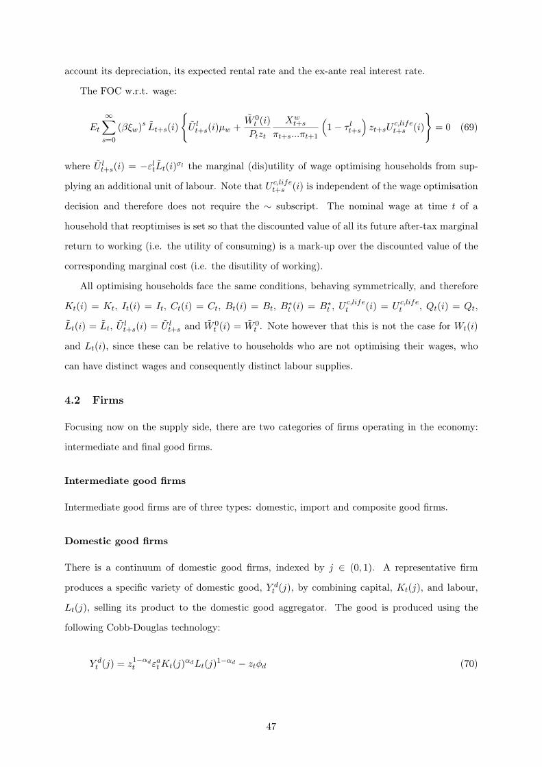
account its depreciation, its expected rental rate and the ex-ante real interest rate.
The FOC w.r.t. wage:
Et
∞∑
s=0
(βξw)s Lt+s(i)
{U l
t+s(i)µw +W 0
t (i)Ptzt
Xwt+s
πt+s...πt+1
(1− τ l
t+s
)zt+sU
c,lifet+s (i)
}= 0 (69)
where U lt+s(i) = −εl
tLt(i)σl the marginal (dis)utility of wage optimising households from sup-
plying an additional unit of labour. Note that U c,lifet+s (i) is independent of the wage optimisation
decision and therefore does not require the ∼ subscript. The nominal wage at time t of a
household that reoptimises is set so that the discounted value of all its future after-tax marginal
return to working (i.e. the utility of consuming) is a mark-up over the discounted value of the
corresponding marginal cost (i.e. the disutility of working).
All optimising households face the same conditions, behaving symmetrically, and therefore
Kt(i) = Kt, It(i) = It, Ct(i) = Ct, Bt(i) = Bt, B∗t (i) = B∗
t , U c,lifet (i) = U c,life
t , Qt(i) = Qt,
Lt(i) = Lt, U lt+s(i) = U l
t+s and W 0t (i) = W 0
t . Note however that this is not the case for Wt(i)
and Lt(i), since these can be relative to households who are not optimising their wages, who
can have distinct wages and consequently distinct labour supplies.
4.2 Firms
Focusing now on the supply side, there are two categories of firms operating in the economy:
intermediate and final good firms.
Intermediate good firms
Intermediate good firms are of three types: domestic, import and composite good firms.
Domestic good firms
There is a continuum of domestic good firms, indexed by j ∈ (0, 1). A representative firm
produces a specific variety of domestic good, Y dt (j), by combining capital, Kt(j), and labour,
Lt(j), selling its product to the domestic good aggregator. The good is produced using the
following Cobb-Douglas technology:
Y dt (j) = z1−αd
t εat Kt(j)αdLt(j)1−αd − ztφd (70)
47

where 0 ≤ αd ≤ 1 is the capital income share, φd is a fixed cost of production and εat is a
domestic, stationary, technology shock. The fixed cost is introduced to ensure zero profits in
the steady-state and is assumed to grow with zt since otherwise it would become irrelevant and
profits would systematically be positive.
Each firm rents capital and hires labour from households in perfectly competitive markets
taking the wage rate, Wt, and the rental rate of capital, Rkt , as given. In their output market,
however, firms work in a monopolistically competitive environment, exploiting the power they
have over the price they charge, P dt (j), arising from the fact that their product is differentiated.
Like in the wages case, the price setting decision is modelled as an indexation variant of the
mechanism spelled out in Calvo (1983). Firms will only update their prices when they receive
a ”price-change signal”, which occurs with a constant (exogenous) probability, 1− ξd, in which
case it sets a new, optimal, price, P dt (j). 1 − ξd is also the proportion of firms that get to
reoptimise and defines the duration of domestic good price contracts, given by 11−ξd
. Firms that
do not receive the ”signal” update their previous period price by partially indexating it to the
current numeraire inflation rate target and to the previous period domestic good inflation rate,
πdt−1. More formally, a domestic good firm which does not get to reoptimise its price in period
t, will set it according to:
P dt (j) = πd
t−1κd
π1−κdt P d
t−1(j) (71)
where 0 ≤ κd ≤ 1 is the degree of domestic good price indexation to its previous period inflation
rate. Using the same reasoning applied to wages, for a firm that reoptimises in t but never again
in the future, the price in any period t + s can be represented by:
P dt+s(j) = Xd
t+sP0,dt (j) (72)
where:
Xdt+s =
1 if s = 0
(πd
t+s−1...πdt
)κd (πt+s...πt+1)1−κd if s > 0
(73)
with Y dt+s(j) being the corresponding production in each period.
All firms choose labour and capital to minimise the cost of producing a certain amount of
48
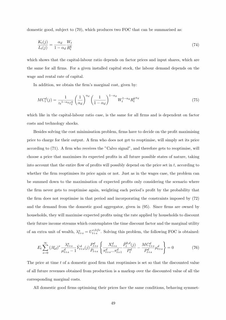
domestic good, subject to (70), which produces two FOC that can be summarised as:
Kt(j)Lt(j)
=αd
1− αd
Wt
Rkt
(74)
which shows that the capital-labour ratio depends on factor prices and input shares, which are
the same for all firms. For a given installed capital stock, the labour demand depends on the
wage and rental rate of capital.
In addition, we obtain the firm’s marginal cost, given by:
MCdt (j) =
1zt
1−αdεat
(1αd
)αd(
11− αd
)1−αd
W 1−αdt Rk
tαd (75)
which like in the capital-labour ratio case, is the same for all firms and is dependent on factor
costs and technology shocks.
Besides solving the cost minimisation problem, firms have to decide on the profit maximising
price to charge for their output. A firm who does not get to reoptimise, will simply set its price
according to (71). A firm who receives the ”Calvo signal”, and therefore gets to reoptimise, will
choose a price that maximises its expected profits in all future possible states of nature, taking
into account that the entire flow of profits will possibly depend on the price set in t, according to
whether the firm reoptimises its price again or not. Just as in the wages case, the problem can
be summed down to the maximisation of expected profits only considering the scenario where
the firm never gets to reoptimise again, weighting each period’s profit by the probability that
the firm does not reoptimise in that period and incorporating the constraints imposed by (72)
and the demand from the domestic good aggregator, given in (95). Since firms are owned by
households, they will maximise expected profits using the rate applied by households to discount
their future income streams which contemplates the time discount factor and the marginal utility
of an extra unit of wealth, λut+s = U c,life
t+s . Solving this problem, the following FOC is obtained:
Et
∞∑
s=0
(βξd)s λu
t+s
µdt+s − 1
Y dt+s(j)
P dt+s
Pt+s
{Xd
t+s
πdt+s...π
dt+1
P 0,dt (j)P d
t
− MCdt+s
P dt+s
µdt+s
}= 0 (76)
The price at time t of a domestic good firm that reoptimises is set so that the discounted value
of all future revenues obtained from production is a markup over the discounted value of all the
corresponding marginal costs.
All domestic good firms optimising their prices face the same conditions, behaving symmet-
49
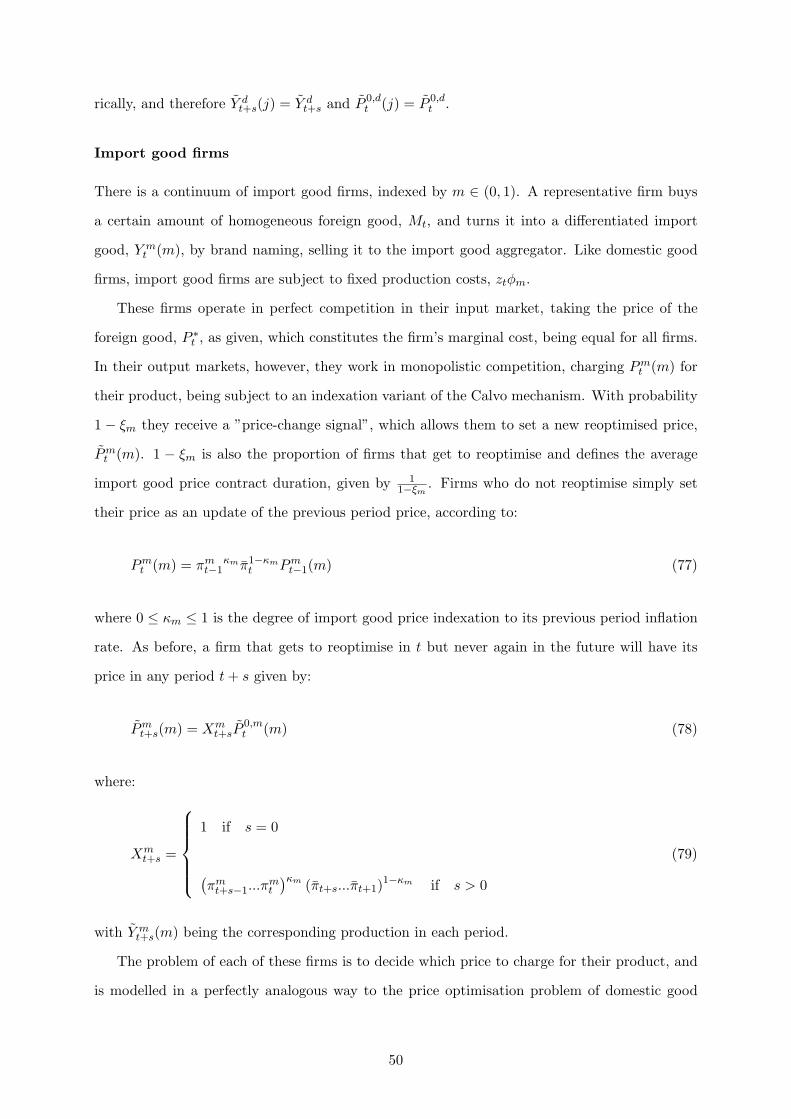
rically, and therefore Y dt+s(j) = Y d
t+s and P 0,dt (j) = P 0,d
t .
Import good firms
There is a continuum of import good firms, indexed by m ∈ (0, 1). A representative firm buys
a certain amount of homogeneous foreign good, Mt, and turns it into a differentiated import
good, Y mt (m), by brand naming, selling it to the import good aggregator. Like domestic good
firms, import good firms are subject to fixed production costs, ztφm.
These firms operate in perfect competition in their input market, taking the price of the
foreign good, P ∗t , as given, which constitutes the firm’s marginal cost, being equal for all firms.
In their output markets, however, they work in monopolistic competition, charging Pmt (m) for
their product, being subject to an indexation variant of the Calvo mechanism. With probability
1− ξm they receive a ”price-change signal”, which allows them to set a new reoptimised price,
Pmt (m). 1 − ξm is also the proportion of firms that get to reoptimise and defines the average
import good price contract duration, given by 11−ξm
. Firms who do not reoptimise simply set
their price as an update of the previous period price, according to:
Pmt (m) = πm
t−1κm π1−κm
t Pmt−1(m) (77)
where 0 ≤ κm ≤ 1 is the degree of import good price indexation to its previous period inflation
rate. As before, a firm that gets to reoptimise in t but never again in the future will have its
price in any period t + s given by:
Pmt+s(m) = Xm
t+sP0,mt (m) (78)
where:
Xmt+s =
1 if s = 0
(πm
t+s−1...πmt
)κm (πt+s...πt+1)1−κm if s > 0
(79)
with Y mt+s(m) being the corresponding production in each period.
The problem of each of these firms is to decide which price to charge for their product, and
is modelled in a perfectly analogous way to the price optimisation problem of domestic good
50

firms, producing the following FOC w.r.t. the price of import good:
Et
∞∑
s=0
(βξm)s λut+s
µmt+s − 1
Y mt+s(m)
Pmt+s
Pt+s
{Xm
t+s
πmt+s...π
mt+1
P 0,mt (m)Pm
t
− MCmt+s
Pmt+s
µmt+s
}= 0 (80)
which is perfectly analogous to the price FOC of domestic good firms, and where:
MCmt+s = P ∗
t+s (81)
All optimising import good firms face the same conditions regarding their decisions, behaving
symmetrically, and therefore Y mt+s(m) = Y m
t+s and P 0,mt (m) = P 0,m
t .
Composite good firm
There is one composite good firm that buys the homogeneous domestic good, Y dt , and the
homogeneous import good, Y mt , from their respective aggregators and combines them to produce
a homogeneous composite good, Y ht ,which is then sold to final good firms. The good is produced
via the following CES technology:
Y ht =
[(1− ωh)
1ϑh+1 Y d
t
ϑhϑh+1 + ω
1ϑh+1
h Y mt
ϑhϑh+1
]ϑh+1
ϑh
(82)
where 0 ≤ ωh ≤ 1 determines the share of import good in the production of composite good and
0 ≤ ϑh < ∞ is the elasticity of substitution between domestic and import goods.
The firm operates in a perfectly competitive environment, taking the prices of the domestic
and import goods, P dt and Pm
t , and the price of its output, P ht , as given.
The firm’s problem is to decide on the combination of domestic and import good that min-
imises the cost of producing a certain quantity of composite good subject to (82), which produces
the following two FOC. The FOC w.r.t. domestic good:
Y dt = (1− ωh)
(P h
t
P dt
)ϑh+1
Y ht (83)
The FOC w.r.t. import good:
Y mt = ωh
(P h
t
Pmt
)ϑh+1
Y ht (84)
51
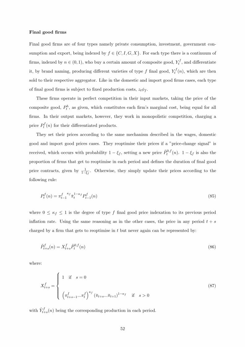
Final good firms
Final good firms are of four types namely private consumption, investment, government con-
sumption and export, being indexed by f ∈ {C, I, G,X}. For each type there is a continuum of
firms, indexed by n ∈ (0, 1), who buy a certain amount of composite good, Y ft , and differentiate
it, by brand naming, producing different varieties of type f final good, Y ft (n), which are then
sold to their respective aggregator. Like in the domestic and import good firms cases, each type
of final good firms is subject to fixed production costs, ztφf .
These firms operate in perfect competition in their input markets, taking the price of the
composite good, P ht , as given, which constitutes each firm’s marginal cost, being equal for all
firms. In their output markets, however, they work in monopolistic competition, charging a
price P ft (n) for their differentiated products.
They set their prices according to the same mechanism described in the wages, domestic
good and import good prices cases. They reoptimise their prices if a ”price-change signal” is
received, which occurs with probability 1 − ξf , setting a new price P 0,ft (n). 1 − ξf is also the
proportion of firms that get to reoptimise in each period and defines the duration of final good
price contracts, given by 11−ξf
. Otherwise, they simply update their prices according to the
following rule:
P ft (n) = πf
t−1
κfπ
1−κf
t P ft−1(n) (85)
where 0 ≤ κf ≤ 1 is the degree of type f final good price indexation to its previous period
inflation rate. Using the same reasoning as in the other cases, the price in any period t + s
charged by a firm that gets to reoptimise in t but never again can be represented by:
P ft+s(n) = Xf
t+sP0,ft (n) (86)
where:
Xft+s =
1 if s = 0
(πf
t+s−1...πft
)κf
(πt+s...πt+1)1−κf if s > 0
(87)
with Y ft+s(n) being the corresponding production in each period.
52
The problem of each of these firms is to decide which price to charge for their product, and is
modelled in a perfectly analogous way to the price optimisation problem of domestic and import
good firms, producing the following FOC w.r.t. the price of type f final good:
Et
∞∑
s=0
(βξf )s λut+s
µft+s − 1
Y ft+s(n)
P ft+s
Pt+s
{Xf
t+s
πft+s...π
ft+1
P 0,ft (n)
P ft
− MCft+s
P ft+s
µft+s
}= 0 (88)
whose interpretation is perfectly equivalent to the domestic and import goods Phillips curves
and where:
MCft+s = P h
t+s (89)
All optimising final good firms face the same conditions regarding their decisions, behaving
symmetrically, and therefore Y ft+s(n) = Y f
t+s and P 0,ft (n) = P 0,f
t .
4.3 Aggregators
Aggregators solve the mismatch between the supply of differentiated products and the demand
for homogeneous products. For each type of differentiated product being supplied, there is an
aggregator that buys the different varieties and combines them to produce an homogeneous
product that can satisfy the economy’s demand, using a CES technology. All the aggregators
operate in a perfectly competitive environment both in their input and output markets, and
therefore take the price of both their inputs and output as given.
The labour aggregator buys the different labour varieties, Lt(i), from households and com-
bines them to produce an homogeneous labour input, Lt, which it then sells to the domestic
good firms. The homogeneous labour input is given by:
Lt =(∫ 1
0Lt(i)
1µw di
)µw
(90)
where 1 ≤ µw < ∞ is the wage markup, which is dependent on the elasticity of substitution
between varieties of labour, 0 ≤ ϑw < ∞, such that µw = ϑw+1ϑw
12.
The problem of the labour aggregator is to decide on the combination of different labour
varieties that minimises the cost of producing Lt, subject to (90). This produces the following12We consider the wage markup to be time-invariant, contrary to the other markups, to prevent identification
problems generated by the coexistence of two shocks, the wage markup shock and the labour supply shock, in thelog-linearised wage equation. For a thorough discussion of this, please refer to Adolfson et al. (2005).
53
FOC w.r.t. each variety of labour:
Lt(i) =(
Wt
Wt(i)
) µwµw−1
Lt (91)
The domestic good aggregator buys the different varieties of domestic good, Y dt (j), from the
domestic good firms and combines them to produce an homogeneous domestic good, Y dt , which
it then sells to the composite good firm. The homogeneous domestic good is given by:
Y dt =
(∫ 1
0Y d
t (j)1
µdt dj
)µdt
(92)
where 1 ≤ µdt < ∞ is the domestic good price markup, modelled as a shock, dependent on the
elasticity of substitution between varieties of domestic good, 0 ≤ ϑdt < ∞, such that µd
t = ϑdt +1
ϑdt
.
The problem solved by the domestic good aggregator is perfectly analogous to the one solved
by the labour aggregator, which produces the following FOC w.r.t. each variety of domestic good:
Y dt (j) =
(P d
t
P dt (j)
) µdt
µdt−1
Y dt (93)
The import good aggregator buys the different varieties of import good, Y mt (m), from the
import good firms and combines them to produce an homogeneous import good, Y mt , which is
then sold to the composite good firm. The homogeneous import good is given by:
Y mt =
(∫ 1
0Y m
t (m)1
µmt dm
)µmt
(94)
where 1 ≤ µmt < ∞ is the import good price markup, modelled as a shock, dependent on the
elasticity of substitution between varieties of import good, 0 ≤ ϑmt < ∞, such that µm
t = ϑmt +1ϑm
t.
The problem solved by the import good aggregator is perfectly analogous to the previous
ones, producing the following FOC w.r.t. each variety of import good:
Y mt (m) =
(Pm
t
Pmt (m)
) µmt
µmt −1
Y mt (95)
Finally, we have the final good aggregators. For each type of final good there is an aggregator,
which takes the different varieties of type f final good, Y ft (n), and combines them to produce an
homogeneous type f final good, Y ft , which is then sold to households, the government and the
54

RW for private consumption, investment, government consumption and export purposes. The
homogeneous type f final good is given by:
Y ft =
(∫ 1
0Y f
t (n)1
µft dn
)µft
(96)
where 1 ≤ µft < ∞ is the type f final good price markup, modelled as a shock, dependent on
the elasticity of substitution between varieties of type f final good, 0 ≤ ϑt < ∞, such that
µft = ϑf
t +1
ϑft
.
The type f final good aggregator solves a perfectly analogous problems to the ones already
described, which produces the following FOC w.r.t. each variety of type f final good:
Y ft (n) =
(P f
t
P ft (n)
) µft
µft −1
Y ft (97)
4.4 Rest of the world
The domestic economy’s homogeneous export good is demanded by the RW agents, who combine
it with their own domestic homogeneous good to produce Y ∗t . The RW’s demand for the export
good, Xt, which corresponds to the home economy’s exports, is exogenously given as:
Xt =(
P ∗t
Pt
)ϑ∗+1
Y ∗t (98)
where 0 ≤ ϑ∗ < ∞ is the foreign economy’s elasticity of substitution between the domestic
export good and the RW’s good.
Foreign economy variables (inflation, output and interest rate) are assumed to be exogenously
given as shocks. Furthermore, we assume that there is a stationary asymmetric (or foreign)
technology shock, ζ∗t = z∗tzt
, where z∗t is the permanent technology level abroad, to allow for
temporary differences between domestic and foreign permanent technological progresses.
4.5 Government
The government spends resources on the acquisition of the government consumption good, P gt Gt,
payment of debt services, (Rt−1 − 1)Bt, and transfers to households, TRt, and obtains resources
from taxes, τ ct P c
t Ct + τ lt
∫ 10 Wt(i)Lt(i)di, and debt issuance, Bt.
The government’s primary deficit, i.e. the difference between the government’s current spend-
55

ing and revenue, excluding debt related resources and expenditures, is then given by:
SGprimt = P g
t Gt + TRt − τ ct P c
t Ct − τ lt
∫ 1
0Wt(i)Lt(i)di (99)
The government’s total deficit also includes interest outlays, being given by:
SGtott = SGprim
t + (Rt−1 − 1)Bt (100)
The government’s budget constraint, defining that its total resources must equal its total
expenditures, can then be written as:
Bt+1 + τ ct P c
t Ct + τ lt
∫ 1
0Wt(i)Lt(i)di = Rt−1Bt + TRt + P g
t Gt ⇔ Bt+1 = Bt + SGtott
(101)
To prevent an explosive debt path, a fiscal rule is imposed, acting as a restriction over SGprimt
such that TRt adjusts endogenously to ensure that the debt to Gross Domestic Product (GDP)
ratio converges to a long-term, pre-specified value. The rule is given already in its stationary
form by:
sgprimt
¨gdp= −dg
(bt+1
¨gdp−
(b¨gdp
)tar)(102)
where(
b¨gdp
)taris the target value for the stationary debt to GDP ratio. Whenever the debt
to GDP ratio is above its target value, transfers automatically decrease in order to reduce the
government’s expenditures and consequently minimise its deficit and future period debt.
The fiscal policy variables (taxes and expenditures) are exogenously given as shocks.
4.6 Aggregation
We have by now presented the problems of each agent in the economy, including their individual
restrictions and decision rules. Besides this, we need some aggregation procedures that, when
applied to these equations, allow us to obtain the behaviour of the economy as whole.
Start by recalling that the i indices can be dropped from the households’ expenditure deci-
sions and therefore we can easily define the aggregate demand for consumption good, government
56
bonds, foreign bonds, investment good and the aggregate supply of capital services as:
∫ 1
0Ct(i)di =
∫ 1
0Ctdi = Ct (103)
∫ 1
0Bt(i)di =
∫ 1
0Btdi = Bt (104)
∫ 1
0B∗
t (i)di =∫ 1
0B∗
t di = B∗t (105)
∫ 1
0It(i)di =
∫ 1
0Itdi = It (106)
∫ 1
0Kt(i)di =
∫ 1
0Ktdi = Kt (107)
Next, note that aggregators and the composite good firm have to comply with a zero profit
condition, as they work in perfect competition, and therefore the following equations hold:
WtLt −∫ 1
0Wt(i)Lt(i)di = 0 ⇔ WtLt =
∫ 1
0Wt(i)Lt(i)di (108)
P dt Y d
t −∫ 1
0P d
t (j)Y dt (j)dj = 0 ⇔ P d
t Y dt =
∫ 1
0P d
t (j)Y dt (j)dj (109)
Pmt Y m
t −∫ 1
0Pm
t (m)Y mt (m)dm = 0 ⇔ Pm
t Y mt =
∫ 1
0Pm
t (m)Y mt (m)dm (110)
P ft Y f
t −∫ 1
0P f
t (n)Y ft (n)df = 0 ⇔ P f
t Y ft =
∫ 1
0P f
t (n)Y ft (n)df (111)
P ht Y h
t − P dt Y d
t − Pmt Y m
t = 0 ⇔ P ht Y h
t = P dt Y d
t + Pmt Y m
t (112)
Furthermore, we need to derive the aggregate supply of domestic good, which can be obtained
by using (70), (95), (121) and (122):
Y dt =
(~P d
t
P dt
) µdt
µdt−1
~Y dt (113)
where:
~Y dt =
∫ 1
0Y d
t (j)dj = z1−αdt εa
t Kαdt L1−αd
t − ztφd (114)
57
~P dt =
(∫ 1
0P d
t (j)− µd
tµd
t−1 dj
)−µdt−1
µdt
(115)
Now note that:
~P dt
P dt
= 1 if P dt (j) = P d
t ∀j ⇒ Y dt = ~Y d
t
~P dt
P dt
< 1 if P dt (j1) 6= P d
t (j2) for any j1, j2 ⇒ Y dt < ~Y d
t
Therefore, the supply of domestic good by the domestic good aggregator, Y dt , is not only
a function of what could be produced using the available technology and inputs, given by ~Y dt ,
but also of ~P dt which is an efficiency distortion that arises from the monopoly power held by the
domestic good firms, determining that whenever there is price differentiation, aggregate supply
of domestic good is lower than aggregate output.
Using (59), (90), (91) we obtain the following expression for the aggregate wage:
Wt =[(1− ξw)
(W 0
t
)− 1µw−1 + ξw
(πκw
t−1π1−κwt ζtWt−1
)− 1µw−1
]−(µw−1)
(116)
Performing analogous operations in the case of domestic, import and final goods, we obtain
their respective aggregate prices:
P dt =
[(1− ξd)
(P 0,d
t
)− 1
µdt−1 + ξd
((πd
t−1
)κd
(πt)1−κd P d
t−1
)− 1
µdt−1
]−(µdt−1)
(117)
Pmt =
[(1− ξm)
(P 0,m
t
)− 1µm
t −1 + ξm
((πm
t−1
)κm (πt)1−κm Pm
t−1
)− 1µm
t −1
]−(µmt −1)
(118)
P ft =
[(1− ξf )
(P 0,f
t
)− 1
µft −1 + ξf
((πf
t−1
)κf
(πt)1−κf P f
t−1
)− 1
µft −1
]−(µf
t−1)
(119)
And finally, we consider the aggregate price of composite good, which can be obtained simply
by replacing (83) and (84) in (82) producing:
P ht =
[(1− ωh)
(P d
t
)−ϑh
+ ωh (Pmt )−ϑh
]− 1ϑh
(120)
58

4.7 Market clearing conditions and useful identities
To close the model we also need to consider market clearing conditions, which ensure that the
economy is always in equilibrium. In the labour market, supply by the labour aggregator must
equal aggregate demand by domestic good firms:
Lt =∫ 1
0Lt(j)dj (121)
In the capital market, aggregate supply by households must equal aggregate demand by
domestic good firms:
Kt =∫ 1
0Kt(j)dj (122)
In the domestic and import good markets, supply by the respective aggregators must equal
demand by the composite good firm:
Y dt = (1− ωh)
(P h
t
P dt
)ϑh+1
Y ht (123)
Y mt = ωh
(P h
t
Pmt
)ϑh+1
Y ht = Mt (124)
In the final good market, supply by the private consumption, investment, government con-
sumption and export good aggregators must equal demand by households, the government and
the RW:
Y ct = Ct (125)
Y it = It (126)
Y gt = Gt (127)
Y xt =
(P ∗
t
Pt
)ϑ∗+1
Y ∗t = Xt (128)
In the foreign bond market, households’ aggregate net bond holdings must equal the econ-
omy’s trade net position:
B∗t+1 −R∗
t−1Φ(b∗t , ε
φt−1
)B∗
t = P xt Xt − P ∗
t Mt (129)
59

And finally, in the composite good market, supply of composite good must equal the amount
of production necessary to satisfy the demand for all types of final good:
Y ht = Y c
t + Y it + Y g
t + Y xt = Ct + It + Gt + Xt (130)
Besides the market clearing conditions, it is useful to present some definitions and identities
that are necessary to solve the model. First, consider a measure of GDP, which following
the National Accounts definition corresponds to the sum of demand expenditures, including
consumption taxes and excluding expenditures with imports:
GDPt = PtCt + P it It + P g
t Gt + P xt Xt − P ∗
t Mt (131)
In addition, note that the following identities concerning wages and prices must always hold:
πwt
πt=
wt
wt−1(132)
πit
πt=
pit
pit−1
(133)
where i = d,m, f, h, ∗.Finally, the numeraire price definition is needed, which has already been given in the begin-
ning of this section.
4.8 Shocks
The stochastic behaviour of the model is driven by twenty structural shocks which are all given
by the following univariate representation:
ξit =
(1− ρξi
)ξi + ρξiξi
t−1 + ηξi,t ηξi,t ∼ N(0, σ2ξi) (134)
where all innovations are assumed to be i.i.d. (independent and identically distributed), i ={εi, εc, εφ, εl, εa, µd, µm, µc, µi, µg, µx, π, ζ, ζ∗, π∗, y∗, r∗, τ l, τ c, G
}and E(ξi
t) = ξi. In the cases of{εi, εc, εl, εa
}it is assumed that ξi = 1.
60

5 Estimation of the model for the Portuguese economy
This section provides all the empirical aspects concerning our estimation process, namely issues
related to the data, the calibration/choice of priors and the estimation results, together with
their evaluation. Throughout the whole estimation process, it is assumed that all parameters
and all shocks are independent and therefore no correlation between them is considered.
5.1 Data
To compute the Portuguese economy’s key steady-state ratios we used annual data, over the
period 1988-2007, taken from the annual National Accounts dataset, available from the Statistics
Portugal Institute (INE). To perform the estimation, we used quarterly data, over the same years.
The choice of the period was conditioned by the fact that some of the Portuguese macroeconomic
series chosen for the estimation process have an extremely erroneous behaviour prior to 1988,
which motivated us not to include this period in the sample.
Portuguese data was taken from the “Quarterly Series for the Portuguese Economy: 1977-
2007” published in the Summer 2008 issue of Banco de Portugal’s Economic Bulletin. Euro area
data was taken from the Area Wide Model (AWM) database13, which was originally presented
in Fagan, Henry and Mestre (2001) and has become a standard reference for empirical studies
using euro area data. To our knowledge however, the most recent update is only until 2005Q4.
To obtain data for 2006 and 2007, we recurred to the Eurostat database and used the implied
growth rates in its series to extend the AWM ones.
We chose to match the following set of thirteen variables: GDP inflation, private consumption
good inflation (including taxes), investment good inflation, real wages, real private consumption,
real investment, real GDP, employment, real exports, real imports, nominal interest rate, foreign
real GDP and foreign nominal interest rate. All inflation rates were obtained as the fourth order
difference of the log of their respective deflator. Real wages were obtained by scaling nominal
wages by the private consumption good deflator.
To render the data stationary, we applied an HP-filter with λ = 7680, a value proposed in
Almeida and Felix (2006) for quarterly Portuguese data, and used the detrended series instead
of the original ones. At this point, it is important to refer some problems we encountered
when dealing with the data. We applied several different strategies in the attempt of rendering
it stationary, in particular first-order differentiation and linear detrending. However, due to13The data is available at http://www.eabcn.org/data/awm/index.htm.
61
the highly non-stationary behaviour of Portuguese data, inevitably marked by the economic
instability that the country suffered during a considerable time span, none of the additional
experimented strategies was able to produce ”well-behaved” series, that could be used in the
estimation. The HP filter was indeed the only methodology (among the ones we tried) that
provided a reasonable treatment of the data. We are however, conscious that this method
suffers from some problems, in particular the well-known end-of-sample bias 14.
The vector of variables used in the estimation can then be described by:
Υ′t =
[πd
t πt πit wt Ct It gdpt Lt Xt Mt Rt gdp∗t R∗
t
]HP
The correspondent time series are shown in Figure 1.
5.2 Calibration
As commonly done in the DSGE literature, a number of parameters were calibrated from the
outset, not being included in the estimation process. This procedure helps to cope with the
problem of identification from which DSGE models commonly suffer, arising from the fact that
the variables used in the estimation may contain little information about some of the parameters
of interest. In small scale models this problem may be solved by carefully looking at each
equation, but in medium or large-scale models (which is our case) this task is almost impossible.
Furthermore, incorporating fixed parameters in the estimation process can be viewed as imposing
a very strict prior, being therefore consistent with the Bayesian approach to estimation.
The parameters we chose to calibrate pertain mostly to three aspects: those crucial to
determine the steady-state; those for which we have reliable estimates from other sources; and
those whose values are crucial to replicate the main steady-state key ratios of the Portuguese
economy.
Being a small open economy in the euro area, Portugal’s steady-state real GDP growth and
inflation rate were assumed to be equal to the euro area average. Therefore, ζ was set to 1.005,
which is consistent with the estimate of 2% for the annual euro area potential output growth
presented in Musso and Westermann (2005) and also seems a plausible estimate for Portugal in
view of the results of Almeida and Felix (2006). In addition, π was set to 1.005, in line with the
ECB goal of 2% for the euro area long-run annual inflation rate. The discount rate β was then14For a thorough discussion of the HP filter, please refer to Almeida and Felix (2006).
62
set to 0.999, to produce a steady-state long-run nominal interest rate of 4.5%, in accordance
with Christoffel et al. (2008).
Conditional on the value assumed for ζ, the depreciation rate was calibrated to match the
empirical long-run annual investment to capital ratio of 8%, implying δ = 0.015, i.e. an annual
depreciation rate of 6%. The steady-state government to domestic output ratio, was set to match
its empirical counterpart implying gy = 0.14. The steady-state tax rates were set according to
Almeida et al. (2008), where τ c = 0.304 and τ l = 0.287, and the target debt to GDP ratio,(
b¨gdp
)tar, was set at 60%, the upper bound of the limit imposed the Maastricht Treaty criteria.
The capital income share was then calibrated so that the model key steady-state ratios closely
followed the correspondent ratios in the data, which produced αd = 0.329.
Besides these parameters, which are usually kept fixed in the DSGE literature, we calibrated
four more parameters that ideally would be estimated, but for which unfortunately we were not
able to obtain robust estimates. These include the habit persistence parameter, the inverse of the
elasticity of labour supply and the import and private consumption goods Calvo parameters. The
habit persistence parameter, h, was set at 0.65 and the import good price stickiness parameter,
ξm, at 0.5, based on the prior means in Adolfson, Laseen, Linde and Villani (2007). The inverse
of the elasticity of labour supply, σl, was calibrated at 2 and the private consumption good price
stickiness parameter, ξc, at 0.6, in line with the values used in Almeida et al. (2008).
5.3 Priors
In Table 1 the assumptions concerning the priors are presented, which greatly benefited from
insights from Adolfson, Laseen, Linde and Villani (2007) and Almeida et al. (2008). The first
one corresponds to a model estimated for Sweden (which like Portugal is a small-open economy)
using Bayesian techniques. The second one, constitutes the most recent and comprehensive
DSGE model developed for the Portuguese economy and therefore, although it is calibrated,
constitutes an important reference for this study.
For parameters bounded to be positive, we used the inverse gamma distribution. These
include the standard deviations of shocks, the steady-state markups and the elasticities of sub-
stitution. For the standard deviations of shocks, we had no strong a-priori convictions and
therefore we set priors as harmonised and loose as possible. For most of the shocks, the mean
was set at 0.15, a value that fits into what is usually used in the literature. For the remaining
shocks, the prior mean had to be set at a considerably low level, 0.02, to ensure the success of
63
the numerical optimisation of the posterior kernel. The standard deviations were all set equal to
the means, which produced rather uninformative priors. The prior means for the steady-state
markup values were mostly based on the calibration made in Almeida et al. (2008) being set at
25% in the wages case, 15% in the domestic goods case and 5% in the final goods case. As for
import prices, we considered a markup of 20%, which corresponds to the value used in Adolfson,
Laseen, Linde and Villani (2007). The standard deviations for all of these priors were set at 0.1,
a common value in the literature. Regarding the elasticities of substitution, we assumed prior
means of 0.515 and standard deviations of 0.1 for both Portugal and RW elasticities of substi-
tution between import and domestic goods, which are standard values in the macro literature,
and in the case of the euro area elasticity of substitution corresponds to the calibration done in
Almeida et al. (2008).
Parameters bounded between zero and one were assumed to follow a beta distribution. These
include the shocks autoregressive parameters, the Calvo and indexation parameters underlying
the wage and price-setting decisions and the share of import goods in the production of the
composite good. Concerning the autoregressive parameters, for which we had no a-priori strong
information, priors were completely harmonised, with their mean set at 0.6. The means for the
priors of the non-reoptimisation Calvo probability were set at 0.7 for both wages and prices,
so that the average contract duration is 3 quarters and one month, which is a simple average
of the values implied in the calibration made in Almeida et al. (2008). As for the indexation
parameters, we set all prior means at 0.5, in line with Adolfson, Laseen, Linde and Villani (2007),
and standard errors at 0.1. Finally, we set the prior mean for the share of import good in the
composite good’s production at 0.4, which is an intermediate value between the ones considered
in our two main references. The standard deviation of all these parameters was set at 0.1, which
is in line with what is usually assumed in the DSGE literature.
Finally, for the investment adjustment cost parameter, which is not upper bounded, we
considered a normal distribution. The prior’s mean and standard deviation were set at 7.6 and
1.5, respectively, based on Adolfson, Laseen, Linde and Villani (2007).15Recall that we have modelled the elasticity of substitution in a slightly different way as is usually done in the
DSGE literature, since generally what is considered the elasticity of substitution is considered to be ϑ + 1 andnot just ϑ. Therefore, comparisons with other models’ parameters should take this into account and subtract onefrom other models’ estimates for the elasticities of substitution.
64
5.4 Estimation results and evaluation
The results for the 63 estimated parameters are presented in the right-hand columns of Table
1. The entries in the posterior kernel maximisation columns report the parameters mode and
standard deviation obtained by maximising the posterior kernel. The remaining three columns
contain the mean and the 5 and 95 percentiles of the posterior distributions computed with
the MH algorithm, based on 500000 draws with 5 distinct chains. In the lower part of the
table, we further present the value of the marginal likelihood, computed with both the Laplace
approximation and the Harmonic mean estimator, and the average acceptance rate for each of
the 5 chains of the MH algorithm.
A number of estimation results are noteworthy. Starting with the markups’ steady-state
values, it is possible to see that our prior conviction of low markups in the final goods sector
seems to be confirmed by the data in the case of investment, government consumption and export
goods, for which the posterior mean is close to one, indicating a high degree of competition in
these markets. However, this does not seem to be the case for the private consumption good,
whose steady-state markup is estimated to be quite high, around 60%, suggesting that domestic
households’ ability to substitute among different varieties of private consumption goods is low.
As for import prices, the markup is also estimated to be large, around 37%, which is in line
with the estimates presented in Adolfson, Laseen, Linde and Villani (2007). In the case of wages
and domestic goods, markups are estimated to be 149% and 145%, respectively, which seem
to be quite unreasonable values and should therefore be taken with care. Note however that
the Portuguese labour market is acknowledged to suffer from a deep lack of competition16, and
therefore these results, although implausibly high, seem to go in the right direction.
Regarding the composite good production function parameters, we can see that the elasticity
of substitution between domestic and import goods is close to 0.3 and the ”quasi-share” of import
goods is around 18%. This estimate is in line with the relatively low share of import goods in
final goods’ production assumed in Almeida et al. (2008). As for the euro area’s elasticity of
substitution between their products and the Portuguese ones, results indicate that it is close to
0.3, which is below the assumption made for the prior distribution.
Turning to the model’s frictions, the investment adjustment cost parameter is estimated to
be roughly equal to 8, which is a value commonly found in the literature. Considering the Calvo16This fact has even partly motivated the work by Almeida et al. (2008), whose main focus was to assess the
macroeconomic impacts of a decrease in the labour and nontradable goods markups.
65

stickiness parameters, we can see that prices in the final goods markets are quite sticky, with
average durations of price contracts close to 1.5 years. Wage contracts, in turn, are estimated
to last slightly more than 1 year, while domestic good prices seem to be quite flexible, being
renegotiated every 2.5 quarters. The greater stickiness of wages relative to domestic prices is
a fairly intuitive result, particularly for the Portuguese economy, where wage negotiations are
centralised and negotiated on a yearly basis. The finding that prices in the final good market
are stickier than prices in the domestic goods and labour markets is however at odds with the
calibration in Almeida et al. (2008) and with what is usually obtained in the literature and
should therefore be taken with a grain of salt. As for the indexation parameters, the estimation
results suggest that inflation persistence is the highest for wages, around 63%, and the lowest
for import prices, around 29%, with the remaining prices assuming values between 35% and
49%. These results compare quite favourably with what is usually obtained, particularly in
the wages case, since it is indeed very frequent that the price of labour is the most related to
past inflation among all the prices considered in DSGE models. This makes particular sense in
the Portuguese economy, since wage negotiations are very much based on past inflation figures
(though no formal indexation mechanism exists).
Finally, we consider the persistency and volatility parameters of structural shocks. The
autoregressive parameters are estimated to lie between 0.33, for the import goods price markup,
and 0.86, for the foreign output shock. None of the shocks is excessively persistent, in the sense
that the posterior distribution’s 95 percentile does not exceed 0.92 for any of the shocks, which
gives an indication on the absence of unit roots in these processes. It is interesting to note
that when compared to the closed economy model of Smets and Wouters (2003), our estimates
are considerably lower, while when compared to the open economy model of Adolfson, Laseen,
Linde and Villani (2007) estimates are closer. This seems to be a reasonable feature, from an
economic point of view, since for an open economy there is an extra possibility of propagation of
shocks hitting the economy, and therefore these are likely to be less persistent. Turning to the
estimated standard deviations, it is possible to conclude that the most volatile shocks considered
in the model are those concerning the markups in the final goods markets (with the exception of
private consumption goods), while the least volatile ones are those related to foreign output and
interest rate and the consumption tax rate. However, the posterior distributions of the markup
shocks parameters are rather wide, indicating that there is substantial parameter uncertainty
and that therefore the parameters are poorly identified.
66

Looking at the diagnosis concerning the numerical maximisation of the posterior kernel,
we see that overall they indicate that the optimisation procedure was able to precisely obtain
a robust maximum for the posterior kernel. The corresponding graphs can be seen in the
Appendix, in Figures 9-12.
In Figures 2-5, we present the prior and posterior distributions as well as the mode obtained
with the maximisation of the posterior kernel. We see that the latter coincides with the mode of
the posterior distribution derived from the MH samples, for the great majority of the parameters.
Also, we observe that the patterns of the prior and posterior distributions are not too far from
each other for practically no parameter with the exception of the wages and domestic goods
price markups whose estimates, as we have already discussed, seem to be unreasonably high.
Furthermore, and most importantly, the prior and posterior distributions are reasonably distinct
for the majority of the parameters, suggesting that the observed data does provide additional
information for most parameters and that therefore the obtained results are not solely ”prior
driven”. This is particularly true for the parameters governing the persistence and volatility
of shocks, which is usually the case in DSGE models. The most noticeable exceptions are the
investment, government consumption and export goods markups, together with the government
consumption indexation parameter, whose posterior distributions are essentially equal to their
respective priors. As for the shape of the posteriors, we see that they are all approximately
normal, which is in line with the asymptotic properties of Bayesian estimation.
In Figure 6, the diagnosis for the MH sampling algorithm are shown. The information is
summarised in three graphs, for each parameter, with each graph representing specific con-
vergence measures and having two distinct lines that represent the results within and between
chains. Those measures are related to the analysis of: the parameter mean (designated interval),
the parameter variance (designated m2) and the parameter third moment (designated m3). For
results to be sensible, both lines, for each of the three measures, must become relatively constant
and converge to each other. Furthermore, a diagnosis of the overall convergence is provided,
following exactly the same structure as the diagnosis for each parameter. As can clearly be seen,
overall convergence was achieved, both within and between chains, for all the three moments
under consideration. Analysing the results for each parameter individually, we observe that
most of the parameters do not in fact exhibit convergence problems, notwithstanding the fact
that for some of them this evidence is stronger than for others. The graphs for each individual
parameter are given in the Appendix, in Figures 13-23.
67

Figure 7 displays the estimates of the innovation component of each structural shock. These
appear to respect the i.i.d. properties assumed from the beginning and are centered around
zero, which gives some positive indication on the statistical validity of the estimated model.
To assess the sensitivity of the results to the assumed priors, we changed these in three
distinct ways and re-estimated the model for each of them17. The corresponding results are
presented in Table 2. In Case I, we increased all prior means and standard deviations by 10%.
Comparing the obtained results with those of our benchmark model, presented in Table 1, we
can see that the majority of the estimates did not changed substantially. In Case II, we kept the
prior means unchanged and increased substantially the prior standard deviations, with increases
ranging from 20% to 60%. Although results exhibit a more substantial change than in Case I,
the overall conclusions remained broadly the same as the ones of the benchmark model. We can
therefore conclude that for reasonable changes in the values of the priors mean and standard
deviation, quantitative results are somewhat sensible but the overall qualitative results are quite
robust. Finally, in Case III, we replaced some of the assumed prior shapes by the uniform
distribution, which amounts to considering an uninformative prior. In this case, with only a
small number of exceptions, the estimation produced radically different results, implausible in
many cases, indicating that, as expected, the shape provided by the priors in the benchmark
model is in fact crucial for the results.
Turning now to the assessment of the absolute fit of the model, we start by inspecting the
overall fit, given by the one step ahead estimates produced by the Kalman filter. These are
presented in Figure 1, for each of the thirteen variables used in the estimation. As can easily be
seen, the obtained estimates are quite close to the true data, indicating that the estimated model
is able to fit the data well. Furthermore, we considered a set of relevant statistics computed with
the Kalman filter estimates and compared them with the ones computed with the real observed
data, namely: the mean, the variance, the cross-(contemporary)correlation coefficients and the
autocorrelation coefficients. Results are presented in Table 3. In general, the model seems to do
a reasonable job in capturing the empirical regularities of the Portuguese data, in the considered
dimensions.
In addition, we compared the fit of the model relative to two alternative common specifica-
tions of a DSGE model, whose results are presented in Table 4. In the first one, designated by17For this purpose, we did not use the MH sampling mechanism since our focus was mainly the comparison
between point estimates and not the entire posterior distributions. Therefore, the presented estimates only concernthe results of the posterior kernel maximisation and the corresponding Laplace approximation to the marginallikelihood.
68

Case IV, we calibrate the persistence coefficients of the markup shocks to be zero, an assumption
that is relatively common in the DSGE literature. In the second one, we test the relevance of
indexation to past inflation in pricing decisions, by calibrating all the indexation parameter to be
zero. Computing the posterior odds ratio of models IV and V relative to the benchmark model,
we obtain figures smaller than one, indicating that the latest is more likely than the formers18.
As discussed in subsection 3.5., a comparison between our preferred specification of the DSGE
model with other models like, VARs, BVARs, etc., could also be performed. However, due to
space constraints, and since this is not at the core of our objectives, we chose not to present this
exercise and instead relegate it to further research.
Finally, we looked at the IRFs of the model’s variables to temporary shocks of one standard
deviation. For all the 20 shocks under consideration, the model’s variables return to their
steady-state value, reinforcing the conclusion given by the Blanchard-Kahn and rank conditions
that the model is indeed stable. Furthermore, in general, results seem to make sense from an
economic point of view. It is not, however, our objective to thoroughly analyse the economy’s
IRF’s to each of the shocks and therefore, we limit ourselves to presenting the results for the
stationary technology shock, for the sake of exemplification19. This can be seen in Figure 8,
where we present the IRFs and corresponding confidence intervals. As expected, the positive
technology shock has an expansionary effect in the economy, producing a rise in wages, GDP and
all its components. Furthermore, it leads to an initial decrease of inflation, due to the decrease
in production costs induced by the increase in productivity, which is however soon supplanted
by the inflationary pressures created by the additional demand and the cost pressure created
by the wages increase. Following the increase in inflation, and since the nominal interest rate is
fixed, the real interest rate experiences a decline.
6 Conclusions and directions for further work
In this study, we discuss the development and estimation of New-Keynesian DSGE models and
provide an application by constructing a model of this type and estimating it for the Portuguese
economy, using Bayesian techniques.
DSGE models are currently a central piece of macroeconometric modelling state of the art,
being used or under development in most policy making and academic institutions. Among the18For the computation of all posterior odds ratios, we considered the prior odds ratio to be one.19The IRFs for all the other shocks are available from the author, upon request.
69

several techniques used to estimate these models, the Bayesian approach has emerged as the
most fruitful one and has been widely adopted in the most recent years. Despite the importance
assumed by these topics in modern macroeconometrics, no attempt had yet been made (to the
best of our knowledge) to explore them for the Portuguese economy, which was certainly a
major flaw in the modelling of the country’s macroeconomic fluctuations20. We consider our
work to be a first step in filling out this gap and hope that it can contribute to a new strategy in
modelling Portugal’s business cycle, in line with the one already in use in many countries and,
in particular, in a considerable number of euro area member states.
Overall, we consider the estimation results to be satisfactory. The diagnostic measures seem
to indicate that the estimation is robust in the majority of its fields, in particular in what
concerns the quality of the numerical posterior kernel maximisation and the convergence of the
MH algorithm. The data seems to be reasonably informative about most of the parameters
and the fit of the model to the observed data set is quite good. The obtained estimates for
the parameters of interest are generally in line with the available literature and, in most cases,
seem to make sense from an economic point of view. Among them, we consider that some are
particularly noteworthy. Firstly, the finding of low markups in the final goods sector, indicating a
high degree of competition in these markets, while the opposite seems to occur in the labour and
intermediate goods sectors, a result that is in line with Almeida et al. (2008). Secondly, wages
are estimated to be stickier than intermediate goods prices, with average contract durations of 4
and 2.5 quarters, respectively, which is in consensus with what is usually found in the literature.
Thirdly, all prices exhibit a considerable degree of indexation to past inflation, particulary wages,
which seem to be considerably backward looking, a result that seems to make sense for the labour
market, since wage negotiations usually take into account on past inflation developments.
It must be noted, however, that the estimation was naturally not free from problems. Several
difficulties were encountered in the treatment of the data, obliging us to use filtered data, which is
recognised to be subject to caveats. Also, despite the overall quality of the diagnostic measures,
this was not a homogeneous result, with some parameters appearing to be estimated in a poorer
way than others. Particularly, in the case of the wages and domestic good price markups, results
seem to be implausibly high. Furthermore, although the data was informative in the majority of
the cases, some estimates seemed to be reasonably influenced by the chosen priors, an influence
that ideally should be as small as possible. Finally, we were not able to estimate all the desired20Note that we are referring to the estimation of a New-Keynesian DSGE model with Bayesian techniques and
not to the subject of DSGE models as a whole. For a detailed discussion of this, please refer to Section 2.
70

parameters in a robust way, which obliged us to proceed with their calibration.
The existence of these caveats indicates that our analysis needs to be further improved in a
number of dimensions. Their importance is, however, as in any estimation procedure, difficult to
assess. We believe, that the balance is certainly positive and consider that our work has shown
that the estimation of a New-Keynesian DSGE model for Portugal, using Bayesian techniques,
can provide useful insights into the characteristics of the Portuguese economy and an empirically
valid tool for the modelling of Portuguese macroeconomic fluctuations.
In the future, we would like to consider some additional aspects not covered in this study, to
further enhance the possibilities surrounding the estimation of a New-Keynesian DSGE model
for the Portuguese economy and hopefully overcome some of the caveats we encountered in
our work. In particular, we would like to re-estimate the model using unfiltered data to check
the robustness of our results and possibly obtain reliable estimates for the parameters that we
have not been able to estimate. Furthermore, we consider that it would be interesting to apply
the strategy followed in Adolfson, Laseen, Linde and Villani (2007) of modelling the fiscal and
foreign variables autonomously, as SVARs, since this would allow to considerably reduce the
”estimation burden” we have imposed on the current model, which is prone to generate identi-
fication problems. In addition, we would like the consider the DSGE-VAR approach explored
in Del Negro and Schorfheide (2004) and Del Negro et al. (2005), which seems to be one of
the most promising ways of bringing stylised macroeconomic models to the data. Finally, a
more comprehensive analysis of the model’s properties could be performed by comparing it to
other, benchmark, models such as VARs and BVARs, considering, among other things, their
forecasting abilities.
References
Abel, A. (1990), ‘Asset prices under habit formation and catching up with the joneses’, The
American Economic Review Vol. 80 (2).
Adolfson, M., Laseen, S., Linde, J. and Villani, M. (2005), ‘Bayesian estimation of an open
economy DSGE model with incomplete pass-through’, Sveriges Riksbank - working papers
series No. 179.
Adolfson, M., Laseen, S., Linde, J. and Villani, M. (2007), ‘Evaluating an estimated new key-
nesian small open economy model’, Sveriges Riksbank - working papers series No. 203.
71
Adolfson, M., Linde, J. and Villani, M. (2007), ‘Forecasting performance of an open economy
DSGE model’, Econometric Reviews Vol. 26 (2-4).
Almeida, V., Castro, G. and Felix, R. (2008), ‘Improving competition in the non-tradable goods
and labour markets: the Portuguese case’, Banco de Portugal - working papers series No.
16.
Almeida, V. and Felix, R. (2006), ‘Computing potential output and the output-gap for the
Portuguese economy’, Banco de Portugal - Economic bulletin Autumn 2006.
Altig, D., Christiano, L., Eichenbaum, M. and Linde, J. (2005), ‘Firm-specific capital, nominal
rigidities and the business cycle’, National Bureau of Economic Research - working papers
series No. 11034.
Alves, N., Gomes, S. and Sousa, J. (2007), ‘An open economy model of the euro area and the
US’, Banco de Portugal - working papers series No. 18.
An, S. and Schorfheide, F. (2007), ‘Bayesian analysis of DSGE models’, Econometric Reviews
Vol. 26 (2).
Avouyi-Dovi, S., Matheron, J. and Feve, P. (2007), ‘DSGE models and their importance to
central banks’, Banque de France - Bulletin digest No. 165.
Bayoumi, T. (2004), ‘GEM a new international macroeconomic model’, International Monetary
Fund - occasional papers series No. 239.
Benigno, P. (2001), ‘Price stability with imperfect financial integration’, New York University -
Manuscript .
Blanchard, O. and Kahn, C. (1980), ‘The solution of linear difference models under rational
expectations’, Econometrica Vol. 48 (5).
Calvo, G. (1983), ‘Staggered prices in a utility-maximising framework’, Journal of Monetary
Economics Vol. 12.
Canova, F. (1994), ‘Statistical inference in calibrated models’, Journal of Applied Econometrics
Vol. 9.
Canova, F. (2007a), ‘Back to square one: identification issues in DSGE models’, Banco de
Espana - documentos de trabajo No. 0715.
72
Canova, F. (2007b), Methods for applied macroeconomic research, Princeton University Press.
Christiano, L. (2002), ‘Solving dynamic equilibrium models by a method of undetermined coef-
ficients’, Computational Economics Vol. 20 (1-2).
Christiano, L. and Eichenbaum, M. (1990), ‘Current real business cycle theories and aggregate
labor market fluctuations’, Federal Reserve Bank of Minneapolis - Intitute for Empirical
Macroeconomics - Discussion papers series No. 24.
Christiano, L., Eichenbaum, M. and Evans, C. (2005), ‘Nominal rigiditis and the dynamic effects
of a shock to monetary policy’, Journal of Political Economy Vol. 113 (1).
Christoffel, K., Coenen, G. and Warne, A. (2008), ‘The new area-wide model of the euro area: a
micro-founded open-economy model for forecasting and policy analysis’, European Central
Bank - working papers series No. 944.
Dejong, D. and Dave, C. (2009), Structural macroeconometrics, Princeton University Press.
DeJong, D., Ingram, B. and Whiteman, C. (2000), ‘A bayesian approach to dynamic macroeco-
nomics’, Journal of Econometrics Vol. 98.
Del Negro, M. and Schorfheide, F. (2004), ‘Priors from general equilibrium models for VARS’,
International Economic Review Vol. 45 (2).
Del Negro, M. and Schorfheide, F. (2008), ‘Forming priors for DSGE models (and how it affects
the assessment of nominal rigidities)’, Journal of Monetary Economics Vol. 55 (7).
Del Negro, M., Schorfheide, F., Smets, F. and Wouters, R. (2005), ‘On the fit and forecasting
performance of new keynesian models’, European Central Bank - working papers series No.
491.
Erceg, C., Henderson, D. and Levin, A. (2000), ‘Optimal monetary policy with staggered wage
and price contracts’, Journal of Monetary Economics Vol. 46.
Fagan, G., Gaspar, V. and Pereira, A. (2004), ‘Macroeconomic adjustment to structural change
(in Monetary Strategies for Joining the Euro)’, Edward Elgar .
Fagan, G., Henry, J. and Mestre, R. (2001), ‘An area-wide model (AWM) for the euro area’,
European Central Bank - working papers series No. 42.
73

Fernandez-Villaverde, J. and Rubio-Ramirez, J. (2004), ‘Comparing dynamic equilibrium models
to data, a bayesian approach’, Journal of Econometrics Vol. 123.
Gali, J. (2008), Monetary policy, inflation, and the business cycle: an introduction to the New
Keynesian framework, Princeton University Press.
Geweke, J. (1999), ‘Using simulation methods for bayesian econometric models: inference, de-
velopment and communication’, Econometric Reviews Vol. 18 (1).
Geweke, J. (2006), ‘Computational experiments and reality’, University of Iowa - Working paper
.
Gomes, S. and Sousa, J. (2007), ‘DSGE models for policy advice - an ilustration with a closed
economy model of the euro area’, Banco de Portugal - Briefing memo No. 13.
Griffoli, T. (2007), An introduction to the solution and estimation of DSGE models, Available
at the Dynare site.
Hamilton, J. (1994), Time series analysis, Princeton University Press.
Hayashi, F. (2000), Econometrics, Princeton University Press.
Ireland, P. (2001), ‘Sticky price models of the business cycle: specification and stability’, Journal
of Monetary Economics Vol. 47.
Iskrev, N. (2009), ‘Local identification in DSGE models’, Banco de Portugal - working papers
series No. 7.
Juillard, M., Kamenik, O., Kumhof, M. and Laxton, D. (2006), ‘Measures of potential from an
estimated DSGE model of the united states’, Czech National Bank - working papers series
No. 11.
Kilponen, J. and Ripatti, A. (2006), ‘Labour and product market competition in a small open
economy: simulation results using a DGE model of the Finnish economy’, Bank of Finland
- Discussion papers series No. 5.
Kim, J. (2000), ‘Constructing and estimating a realistic optimizing model of monetary policy’,
Journal of Monetary Economics Vol. 45.
74

King, R. (1991), ‘Money and business cycles’, Federal Reserve Bank of San Francisco - Proceed-
ings .
Klein, P. (2000), ‘Using the generalized schur form to solve a multivariate linear rational expec-
tations model’, Journal of Economic Dynamics and Control Vol. 24.
Kremer, J., Lombardo, G., von Thadden, L. and Werner, T. (2006), ‘Dynamic stochastic general
equilibrium models as a tool for policy analysis’, CESifo - Economic studies Vol. 52 (4).
Kumhof, M. and Laxton, D. (2007), ‘A party without a hangover?’, International Monetary
Fund - Research papers series No. 43.
Kydland, F. and Prescott, E. (1982), ‘Time to build and aggregate fluctuations’, Econometrica
Vol. 50 (6).
Lutkepohl, H. and Kratzig, M. (2004), Applied time series econometrics, Cambridge University
Press.
Lucas, R. (1976), ‘Econometric policy evaluation: a critique’, Carnegie-Rochester Conference
Series on Public Policy No. 1.
Milani, F. and Poirier, D. (2007), ‘Econometric issues in DSGE models’, Econometric Reviews
Vol. 26.
Musso, A. and Westermann, T. (2005), ‘Assessing potential output in the euro area: a growth
accounting perspective’, European Central Bank - Occasional papers series No. 22.
Pereira, A. and Rodrigues, P. (2000), ‘On the impact of a tax reform package in Portugal’,
Manuscript.
Pytlarczyk, E. (2005), ‘An estimated DSGE model for the German economy within the euro
area’, Deutsche Bundesbank - Discussion papers series 1: economic studies No. 33.
Rabanal, P. and Rubio-Ramırez, J. (2005), ‘Comparing new keynesian models of the business
cycle: a bayesian approach’, Journal of Monetary Economics Vol. 52.
Rotemberg, J. and Woodford, M. (1995), ‘Dynamic general equilibrium models with imperfectly
competitive product markets’, National Bureau of Economic Research - working papers
series No. 4502.
75

Schmitt-Grohe, S. and Uribe, M. (2001), ‘Stabilization policy and the costs of dollarization’,
Journal of Money, Credit, and Banking Vol. 33.
Schmitt-Grohe, S. and Uribe, M. (2003), ‘Closing small open economy models’, Journal of
International Economics Vol. 61.
Silvano, A. (2006), ‘Real business cycles in a small open economy: Portugal 1960-2005’,
Manuscript, Master thesis in Applied Econometrics and Forecasting, ISEG .
Sims, C. (1980), ‘Macroeconomics and reality’, Econometrica Vol. 48.
Sims, C. (2002), ‘Solving linear rational expectations models’, Computational Economics Vol.
20 (1-2).
Smets, F. and Wouters, R. (2003), ‘An estimated dynamic stochastic general equilibrium model
of the euro area’, Journal of the European Economic Association Vol. 1 (5).
Smets, F. and Wouters, R. (2005), ‘Comparing shocks and frictions in US and euro area business
cycles: a bayesian DSGE approach’, Journal of Applied Econometrics Vol. 20.
Welch, G. and Bishop, G. (2001), ‘An introduction to the Kalman filter’, University of North
Carolina at Chapel Hill - Department of Computer Science Manuscript.
Woodford, M. (2003), Interest and prices: foundations of a theory of monetary policy, Princeton
University Press.
Wooldridge, J. (2003), Introductory econometrics - a modern approach, South-Western - Thom-
son.
76
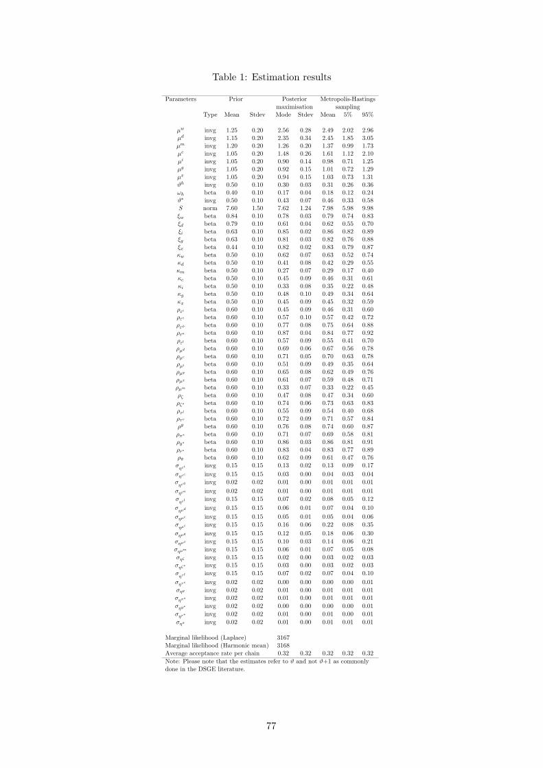
Table 1: Estimation results
Parameters Prior Posterior Metropolis-Hastingsmaximisation sampling
Type Mean Stdev Mode Stdev Mean 5% 95%
µw invg 1.25 0.20 2.56 0.28 2.49 2.02 2.96µd invg 1.15 0.20 2.35 0.34 2.45 1.85 3.05µm invg 1.20 0.20 1.26 0.20 1.37 0.99 1.73µc invg 1.05 0.20 1.48 0.26 1.61 1.12 2.10µi invg 1.05 0.20 0.90 0.14 0.98 0.71 1.25µg invg 1.05 0.20 0.92 0.15 1.01 0.72 1.29µx invg 1.05 0.20 0.94 0.15 1.03 0.73 1.31ϑh invg 0.50 0.10 0.30 0.03 0.31 0.26 0.36ωh beta 0.40 0.10 0.17 0.04 0.18 0.12 0.24ϑ∗ invg 0.50 0.10 0.43 0.07 0.46 0.33 0.58S norm 7.60 1.50 7.62 1.24 7.98 5.98 9.98ξw beta 0.84 0.10 0.78 0.03 0.79 0.74 0.83ξd beta 0.79 0.10 0.61 0.04 0.62 0.55 0.70ξi beta 0.63 0.10 0.85 0.02 0.86 0.82 0.89ξg beta 0.63 0.10 0.81 0.03 0.82 0.76 0.88ξx beta 0.44 0.10 0.82 0.02 0.83 0.79 0.87κw beta 0.50 0.10 0.62 0.07 0.63 0.52 0.74κd beta 0.50 0.10 0.41 0.08 0.42 0.29 0.55κm beta 0.50 0.10 0.27 0.07 0.29 0.17 0.40κc beta 0.50 0.10 0.45 0.09 0.46 0.31 0.61κi beta 0.50 0.10 0.33 0.08 0.35 0.22 0.48κg beta 0.50 0.10 0.48 0.10 0.49 0.34 0.64κx beta 0.50 0.10 0.45 0.09 0.45 0.32 0.59ρεi beta 0.60 0.10 0.45 0.09 0.46 0.31 0.60ρεc beta 0.60 0.10 0.57 0.10 0.57 0.42 0.72ρεφ beta 0.60 0.10 0.77 0.08 0.75 0.64 0.88ρεa beta 0.60 0.10 0.87 0.04 0.84 0.77 0.92ρεl beta 0.60 0.10 0.57 0.09 0.55 0.41 0.70ρµd beta 0.60 0.10 0.69 0.06 0.67 0.56 0.78ρµc beta 0.60 0.10 0.71 0.05 0.70 0.63 0.78ρµi beta 0.60 0.10 0.51 0.09 0.49 0.35 0.64ρµg beta 0.60 0.10 0.65 0.08 0.62 0.49 0.76ρµx beta 0.60 0.10 0.61 0.07 0.59 0.48 0.71ρµm beta 0.60 0.10 0.33 0.07 0.33 0.22 0.45ρζ beta 0.60 0.10 0.47 0.08 0.47 0.34 0.60ρζ∗ beta 0.60 0.10 0.74 0.06 0.73 0.63 0.83ρτ l beta 0.60 0.10 0.55 0.09 0.54 0.40 0.68ρτc beta 0.60 0.10 0.72 0.09 0.71 0.57 0.84ρg beta 0.60 0.10 0.76 0.08 0.74 0.60 0.87ρπ∗ beta 0.60 0.10 0.71 0.07 0.69 0.58 0.81ρy∗ beta 0.60 0.10 0.86 0.03 0.86 0.81 0.91ρr∗ beta 0.60 0.10 0.83 0.04 0.83 0.77 0.89ρπ beta 0.60 0.10 0.62 0.09 0.61 0.47 0.76σ
ηεi invg 0.15 0.15 0.13 0.02 0.13 0.09 0.17σηεc invg 0.15 0.15 0.03 0.00 0.04 0.03 0.04σ
ηεφ invg 0.02 0.02 0.01 0.00 0.01 0.01 0.01σηεa invg 0.02 0.02 0.01 0.00 0.01 0.01 0.01σ
ηεl invg 0.15 0.15 0.07 0.02 0.08 0.05 0.12σ
ηµd invg 0.15 0.15 0.06 0.01 0.07 0.04 0.10σηµc invg 0.15 0.15 0.05 0.01 0.05 0.04 0.06σ
ηµi invg 0.15 0.15 0.16 0.06 0.22 0.08 0.35σηµg invg 0.15 0.15 0.12 0.05 0.18 0.06 0.30σηµx invg 0.15 0.15 0.10 0.03 0.14 0.06 0.21σηµm invg 0.15 0.15 0.06 0.01 0.07 0.05 0.08σηζ invg 0.15 0.15 0.02 0.00 0.03 0.02 0.03σηζ∗ invg 0.15 0.15 0.03 0.00 0.03 0.02 0.03σ
ητl invg 0.15 0.15 0.07 0.02 0.07 0.04 0.10σητc invg 0.02 0.02 0.00 0.00 0.00 0.00 0.01σηg invg 0.02 0.02 0.01 0.00 0.01 0.01 0.01σηπ∗ invg 0.02 0.02 0.01 0.00 0.01 0.01 0.01σηy∗ invg 0.02 0.02 0.00 0.00 0.00 0.00 0.01σηr∗ invg 0.02 0.02 0.01 0.00 0.01 0.00 0.01σηπ invg 0.02 0.02 0.01 0.00 0.01 0.01 0.01
Marginal likelihood (Laplace) 3167Marginal likelihood (Harmonic mean) 3168Average acceptance rate per chain 0.32 0.32 0.32 0.32 0.32Note: Please note that the estimates refer to ϑ and not ϑ+1 as commonlydone in the DSGE literature.
77
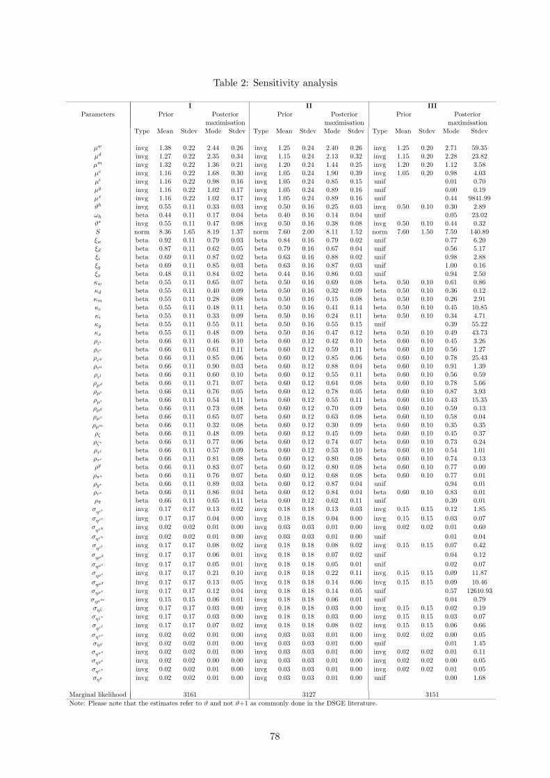
Table 2: Sensitivity analysis
I II IIIParameters Prior Posterior Prior Posterior Prior Posterior
maximisation maximisation maximisationType Mean Stdev Mode Stdev Type Mean Stdev Mode Stdev Type Mean Stdev Mode Stdev
µw invg 1.38 0.22 2.44 0.26 invg 1.25 0.24 2.40 0.26 invg 1.25 0.20 2.71 59.35µd invg 1.27 0.22 2.35 0.34 invg 1.15 0.24 2.13 0.32 invg 1.15 0.20 2.28 23.82µm invg 1.32 0.22 1.36 0.21 invg 1.20 0.24 1.44 0.25 invg 1.20 0.20 1.12 3.58µc invg 1.16 0.22 1.68 0.30 invg 1.05 0.24 1.90 0.39 invg 1.05 0.20 0.98 4.03µi invg 1.16 0.22 0.98 0.16 invg 1.05 0.24 0.85 0.15 unif 0.01 0.70µg invg 1.16 0.22 1.02 0.17 invg 1.05 0.24 0.89 0.16 unif 0.00 0.19µx invg 1.16 0.22 1.02 0.17 invg 1.05 0.24 0.89 0.16 unif 0.44 9841.99ϑh invg 0.55 0.11 0.33 0.03 invg 0.50 0.16 0.25 0.03 invg 0.50 0.10 0.30 2.89ωh beta 0.44 0.11 0.17 0.04 beta 0.40 0.16 0.14 0.04 unif 0.05 23.02ϑ∗ invg 0.55 0.11 0.47 0.08 invg 0.50 0.16 0.38 0.08 invg 0.50 0.10 0.44 0.32S norm 8.36 1.65 8.19 1.37 norm 7.60 2.00 8.11 1.52 norm 7.60 1.50 7.59 140.89ξw beta 0.92 0.11 0.79 0.03 beta 0.84 0.16 0.79 0.02 unif 0.77 6.20ξd beta 0.87 0.11 0.62 0.05 beta 0.79 0.16 0.67 0.04 unif 0.56 5.17ξi beta 0.69 0.11 0.87 0.02 beta 0.63 0.16 0.88 0.02 unif 0.98 2.88ξg beta 0.69 0.11 0.85 0.03 beta 0.63 0.16 0.87 0.03 unif 1.00 0.16ξx beta 0.48 0.11 0.84 0.02 beta 0.44 0.16 0.86 0.03 unif 0.94 2.50κw beta 0.55 0.11 0.65 0.07 beta 0.50 0.16 0.69 0.08 beta 0.50 0.10 0.61 0.86κd beta 0.55 0.11 0.40 0.09 beta 0.50 0.16 0.32 0.09 beta 0.50 0.10 0.36 0.12κm beta 0.55 0.11 0.28 0.08 beta 0.50 0.16 0.15 0.08 beta 0.50 0.10 0.26 2.91κc beta 0.55 0.11 0.48 0.11 beta 0.50 0.16 0.41 0.14 beta 0.50 0.10 0.45 10.85κi beta 0.55 0.11 0.33 0.09 beta 0.50 0.16 0.24 0.11 beta 0.50 0.10 0.34 4.71κg beta 0.55 0.11 0.55 0.11 beta 0.50 0.16 0.55 0.15 unif 0.39 55.22κx beta 0.55 0.11 0.48 0.09 beta 0.50 0.16 0.47 0.12 beta 0.50 0.10 0.49 43.73ρεi beta 0.66 0.11 0.46 0.10 beta 0.60 0.12 0.42 0.10 beta 0.60 0.10 0.45 3.26ρεc beta 0.66 0.11 0.61 0.11 beta 0.60 0.12 0.59 0.11 beta 0.60 0.10 0.56 1.27ρεφ beta 0.66 0.11 0.85 0.06 beta 0.60 0.12 0.85 0.06 beta 0.60 0.10 0.78 25.43ρεa beta 0.66 0.11 0.90 0.03 beta 0.60 0.12 0.88 0.04 beta 0.60 0.10 0.91 1.39ρεl beta 0.66 0.11 0.60 0.10 beta 0.60 0.12 0.55 0.11 beta 0.60 0.10 0.56 0.59ρµd beta 0.66 0.11 0.71 0.07 beta 0.60 0.12 0.64 0.08 beta 0.60 0.10 0.78 5.66ρµc beta 0.66 0.11 0.76 0.05 beta 0.60 0.12 0.78 0.05 beta 0.60 0.10 0.87 3.93ρµi beta 0.66 0.11 0.54 0.11 beta 0.60 0.12 0.55 0.11 beta 0.60 0.10 0.43 15.35ρµg beta 0.66 0.11 0.73 0.08 beta 0.60 0.12 0.70 0.09 beta 0.60 0.10 0.59 0.13ρµx beta 0.66 0.11 0.65 0.07 beta 0.60 0.12 0.63 0.08 beta 0.60 0.10 0.58 0.04ρµm beta 0.66 0.11 0.32 0.08 beta 0.60 0.12 0.30 0.09 beta 0.60 0.10 0.35 0.35ρζ beta 0.66 0.11 0.48 0.09 beta 0.60 0.12 0.45 0.09 beta 0.60 0.10 0.45 0.37ρζ∗ beta 0.66 0.11 0.77 0.06 beta 0.60 0.12 0.74 0.07 beta 0.60 0.10 0.73 0.24ρτ l beta 0.66 0.11 0.57 0.09 beta 0.60 0.12 0.53 0.10 beta 0.60 0.10 0.54 1.01ρτc beta 0.66 0.11 0.81 0.08 beta 0.60 0.12 0.80 0.08 beta 0.60 0.10 0.74 0.13ρg beta 0.66 0.11 0.83 0.07 beta 0.60 0.12 0.80 0.08 beta 0.60 0.10 0.77 0.00ρπ∗ beta 0.66 0.11 0.76 0.07 beta 0.60 0.12 0.68 0.08 beta 0.60 0.10 0.77 0.01ρy∗ beta 0.66 0.11 0.89 0.03 beta 0.60 0.12 0.87 0.04 unif 0.94 0.01ρr∗ beta 0.66 0.11 0.86 0.04 beta 0.60 0.12 0.84 0.04 beta 0.60 0.10 0.83 0.01ρπ beta 0.66 0.11 0.65 0.11 beta 0.60 0.12 0.62 0.11 unif 0.39 0.01σ
ηεi invg 0.17 0.17 0.13 0.02 invg 0.18 0.18 0.13 0.03 invg 0.15 0.15 0.12 1.85σηεc invg 0.17 0.17 0.04 0.00 invg 0.18 0.18 0.04 0.00 invg 0.15 0.15 0.03 0.07σ
ηεφ invg 0.02 0.02 0.01 0.00 invg 0.03 0.03 0.01 0.00 invg 0.02 0.02 0.01 0.60σηεa invg 0.02 0.02 0.01 0.00 invg 0.03 0.03 0.01 0.00 unif 0.01 0.04σ
ηεl invg 0.17 0.17 0.08 0.02 invg 0.18 0.18 0.08 0.02 invg 0.15 0.15 0.07 0.42σ
ηµd invg 0.17 0.17 0.06 0.01 invg 0.18 0.18 0.07 0.02 unif 0.04 0.12σηµc invg 0.17 0.17 0.05 0.01 invg 0.18 0.18 0.05 0.01 unif 0.02 0.07σ
ηµi invg 0.17 0.17 0.21 0.10 invg 0.18 0.18 0.22 0.11 invg 0.15 0.15 0.09 11.87σηµg invg 0.17 0.17 0.13 0.05 invg 0.18 0.18 0.14 0.06 invg 0.15 0.15 0.09 10.46σηµx invg 0.17 0.17 0.12 0.04 invg 0.18 0.18 0.14 0.05 unif 0.57 12610.93σηµm invg 0.15 0.15 0.06 0.01 invg 0.18 0.18 0.06 0.01 unif 0.04 0.79σηζ invg 0.17 0.17 0.03 0.00 invg 0.18 0.18 0.03 0.00 invg 0.15 0.15 0.02 0.19σηζ∗ invg 0.17 0.17 0.03 0.00 invg 0.18 0.18 0.03 0.00 invg 0.15 0.15 0.03 0.07σ
ητl invg 0.17 0.17 0.07 0.02 invg 0.18 0.18 0.08 0.02 invg 0.15 0.15 0.06 0.66σητc invg 0.02 0.02 0.01 0.00 invg 0.03 0.03 0.01 0.00 invg 0.02 0.02 0.00 0.05σηg invg 0.02 0.02 0.01 0.00 invg 0.03 0.03 0.01 0.00 unif 0.01 1.45σηπ∗ invg 0.02 0.02 0.01 0.00 invg 0.03 0.03 0.01 0.00 invg 0.02 0.02 0.01 0.11σηy∗ invg 0.02 0.02 0.00 0.00 invg 0.03 0.03 0.01 0.00 invg 0.02 0.02 0.00 0.05σηr∗ invg 0.02 0.02 0.01 0.00 invg 0.03 0.03 0.01 0.00 invg 0.02 0.02 0.01 0.05σηπ invg 0.02 0.02 0.01 0.00 invg 0.03 0.03 0.01 0.00 unif 0.00 1.68
Marginal likelihood 3161 3127 3151Note: Please note that the estimates refer to ϑ and not ϑ+1 as commonly done in the DSGE literature.
78
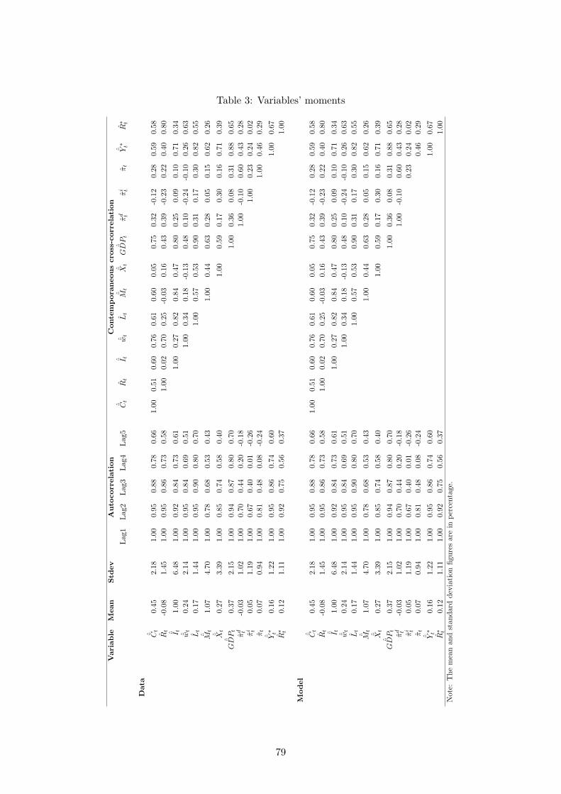
Table 3: Variables’ momentsV
aria
ble
Mea
nStd
evA
uto
corr
elat
ion
Con
tem
por
aneo
us
cros
s-co
rrel
atio
n
Lag
1Lag
2Lag
3Lag
4Lag
5ˆ C
tR
tˆ I t
ˆ wt
Lt
ˆ Mt
ˆ Xt
ˆG
DP
tπ
d tπ
i tπ
tˆ Y∗ t
R∗ t
Dat
aˆ C
t0.
452.
181.
000.
950.
880.
780.
661.
000.
510.
600.
760.
610.
600.
050.
750.
32-0
.12
0.28
0.59
0.58
Rt
-0.0
81.
451.
000.
950.
860.
730.
581.
000.
020.
700.
25-0
.03
0.16
0.43
0.39
-0.2
30.
220.
400.
80ˆ I t
1.00
6.48
1.00
0.92
0.84
0.73
0.61
1.00
0.27
0.82
0.84
0.47
0.80
0.25
0.09
0.10
0.71
0.34
ˆ wt
0.24
2.14
1.00
0.95
0.84
0.69
0.51
1.00
0.34
0.18
-0.1
30.
480.
10-0
.24
-0.1
00.
260.
63L
t0.
171.
441.
000.
950.
900.
800.
701.
000.
570.
530.
900.
310.
170.
300.
820.
55ˆ M
t1.
074.
701.
000.
780.
680.
530.
431.
000.
440.
630.
280.
050.
150.
620.
26ˆ X
t0.
273.
391.
000.
850.
740.
580.
401.
000.
590.
170.
300.
160.
710.
39ˆ
GD
Pt
0.37
2.15
1.00
0.94
0.87
0.80
0.70
1.00
0.36
0.08
0.31
0.88
0.65
πd t
-0.0
31.
021.
000.
700.
440.
20-0
.18
1.00
-0.1
00.
600.
430.
28π
i t0.
051.
191.
000.
670.
400.
01-0
.26
1.00
0.23
0.24
0.02
πt
0.07
0.94
1.00
0.81
0.48
0.08
-0.2
41.
000.
460.
29ˆ Y∗ t
0.16
1.22
1.00
0.95
0.86
0.74
0.60
1.00
0.67
R∗ t
0.12
1.11
1.00
0.92
0.75
0.56
0.37
1.00
Model
ˆ Ct
0.45
2.18
1.00
0.95
0.88
0.78
0.66
1.00
0.51
0.60
0.76
0.61
0.60
0.05
0.75
0.32
-0.1
20.
280.
590.
58R
t-0
.08
1.45
1.00
0.95
0.86
0.73
0.58
1.00
0.02
0.70
0.25
-0.0
30.
160.
430.
39-0
.23
0.22
0.40
0.80
ˆ I t1.
006.
481.
000.
920.
840.
730.
611.
000.
270.
820.
840.
470.
800.
250.
090.
100.
710.
34ˆ w
t0.
242.
141.
000.
950.
840.
690.
511.
000.
340.
18-0
.13
0.48
0.10
-0.2
4-0
.10
0.26
0.63
Lt
0.17
1.44
1.00
0.95
0.90
0.80
0.70
1.00
0.57
0.53
0.90
0.31
0.17
0.30
0.82
0.55
ˆ Mt
1.07
4.70
1.00
0.78
0.68
0.53
0.43
1.00
0.44
0.63
0.28
0.05
0.15
0.62
0.26
ˆ Xt
0.27
3.39
1.00
0.85
0.74
0.58
0.40
1.00
0.59
0.17
0.30
0.16
0.71
0.39
ˆG
DP
t0.
372.
151.
000.
940.
870.
800.
701.
000.
360.
080.
310.
880.
65π
d t-0
.03
1.02
1.00
0.70
0.44
0.20
-0.1
81.
00-0
.10
0.60
0.43
0.28
πi t
0.05
1.19
1.00
0.67
0.40
0.01
-0.2
60.
230.
240.
02π
t0.
070.
941.
000.
810.
480.
08-0
.24
0.46
0.29
ˆ Y∗ t
0.16
1.22
1.00
0.95
0.86
0.74
0.60
1.00
0.67
R∗ t
0.12
1.11
1.00
0.92
0.75
0.56
0.37
1.00
Not
e:T
hem
ean
and
stan
dard
devi
atio
nfig
ures
are
inpe
rcen
tage
.
79
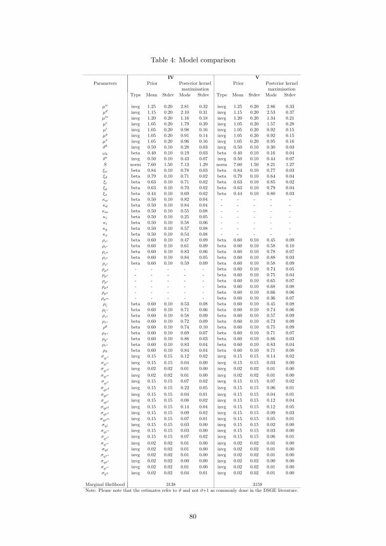
Table 4: Model comparison
IV VParameters Prior Posterior kernel Prior Posterior kernel
maximisation maximisationType Mean Stdev Mode Stdev Type Mean Stdev Mode Stdev
µw invg 1.25 0.20 2.81 0.32 invg 1.25 0.20 2.86 0.33µd invg 1.15 0.20 2.10 0.31 invg 1.15 0.20 2.53 0.37µm invg 1.20 0.20 1.16 0.18 invg 1.20 0.20 1.34 0.21µc invg 1.05 0.20 1.79 0.39 invg 1.05 0.20 1.57 0.28µi invg 1.05 0.20 0.98 0.16 invg 1.05 0.20 0.92 0.15µg invg 1.05 0.20 0.91 0.14 invg 1.05 0.20 0.92 0.15µx invg 1.05 0.20 0.96 0.16 invg 1.05 0.20 0.95 0.16ϑh invg 0.50 0.10 0.28 0.03 invg 0.50 0.10 0.30 0.03ωh beta 0.40 0.10 0.19 0.03 beta 0.40 0.10 0.16 0.04ϑ∗ invg 0.50 0.10 0.43 0.07 invg 0.50 0.10 0.44 0.07S norm 7.60 1.50 7.13 1.29 norm 7.60 1.50 8.21 1.27ξw beta 0.84 0.10 0.78 0.03 beta 0.84 0.10 0.77 0.03ξd beta 0.79 0.10 0.71 0.02 beta 0.79 0.10 0.64 0.04ξi beta 0.63 0.10 0.71 0.02 beta 0.63 0.10 0.85 0.02ξg beta 0.63 0.10 0.70 0.02 beta 0.63 0.10 0.79 0.04ξx beta 0.44 0.10 0.69 0.02 beta 0.44 0.10 0.80 0.03κw beta 0.50 0.10 0.82 0.04 - - - - -κd beta 0.50 0.10 0.84 0.04 - - - - -κm beta 0.50 0.10 0.55 0.08 - - - - -κc beta 0.50 0.10 0.25 0.05 - - - - -κi beta 0.50 0.10 0.58 0.06 - - - - -κg beta 0.50 0.10 0.57 0.08 - - - - -κx beta 0.50 0.10 0.54 0.08 - - - - -ρεi beta 0.60 0.10 0.47 0.09 beta 0.60 0.10 0.45 0.09ρεc beta 0.60 0.10 0.61 0.09 beta 0.60 0.10 0.58 0.10ρεφ beta 0.60 0.10 0.83 0.06 beta 0.60 0.10 0.78 0.07ρεa beta 0.60 0.10 0.84 0.05 beta 0.60 0.10 0.88 0.03ρεl beta 0.60 0.10 0.59 0.09 beta 0.60 0.10 0.58 0.09ρµd - - - - - beta 0.60 0.10 0.74 0.05ρµc - - - - - beta 0.60 0.10 0.75 0.04ρµi - - - - - beta 0.60 0.10 0.65 0.07ρµg - - - - - beta 0.60 0.10 0.68 0.08ρµx - - - - - beta 0.60 0.10 0.66 0.06ρµm - - - - - beta 0.60 0.10 0.36 0.07ρζ beta 0.60 0.10 0.53 0.08 beta 0.60 0.10 0.45 0.08ρζ∗ beta 0.60 0.10 0.71 0.06 beta 0.60 0.10 0.74 0.06ρτ l beta 0.60 0.10 0.58 0.09 beta 0.60 0.10 0.57 0.09ρτc beta 0.60 0.10 0.72 0.09 beta 0.60 0.10 0.73 0.09ρg beta 0.60 0.10 0.74 0.10 beta 0.60 0.10 0.75 0.09ρπ∗ beta 0.60 0.10 0.69 0.07 beta 0.60 0.10 0.71 0.07ρy∗ beta 0.60 0.10 0.86 0.03 beta 0.60 0.10 0.86 0.03ρr∗ beta 0.60 0.10 0.83 0.04 beta 0.60 0.10 0.83 0.04ρπ beta 0.60 0.10 0.84 0.04 beta 0.60 0.10 0.71 0.08σ
ηεi invg 0.15 0.15 0.12 0.02 invg 0.15 0.15 0.14 0.02σηεc invg 0.15 0.15 0.04 0.00 invg 0.15 0.15 0.03 0.00σ
ηεφ invg 0.02 0.02 0.01 0.00 invg 0.02 0.02 0.01 0.00σηεa invg 0.02 0.02 0.01 0.00 invg 0.02 0.02 0.01 0.00σ
ηεl invg 0.15 0.15 0.07 0.02 invg 0.15 0.15 0.07 0.02σ
ηµd invg 0.15 0.15 0.22 0.05 invg 0.15 0.15 0.06 0.01σηµc invg 0.15 0.15 0.04 0.01 invg 0.15 0.15 0.04 0.01σ
ηµi invg 0.15 0.15 0.08 0.02 invg 0.15 0.15 0.12 0.04σηµg invg 0.15 0.15 0.14 0.04 invg 0.15 0.15 0.12 0.05σηµx invg 0.15 0.15 0.09 0.02 invg 0.15 0.15 0.09 0.03σηµm invg 0.15 0.15 0.07 0.01 invg 0.15 0.15 0.05 0.01σηζ invg 0.15 0.15 0.03 0.00 invg 0.15 0.15 0.02 0.00σηζ∗ invg 0.15 0.15 0.03 0.00 invg 0.15 0.15 0.03 0.00σ
ητl invg 0.15 0.15 0.07 0.02 invg 0.15 0.15 0.06 0.01σητc invg 0.02 0.02 0.01 0.00 invg 0.02 0.02 0.01 0.00σηg invg 0.02 0.02 0.01 0.00 invg 0.02 0.02 0.01 0.00σηπ∗ invg 0.02 0.02 0.01 0.00 invg 0.02 0.02 0.01 0.00σηy∗ invg 0.02 0.02 0.00 0.00 invg 0.02 0.02 0.00 0.00σηr∗ invg 0.02 0.02 0.01 0.00 invg 0.02 0.02 0.01 0.00σηπ invg 0.02 0.02 0.04 0.01 invg 0.02 0.02 0.01 0.00
Marginal likelihood 3138 3159Note: Please note that the estimates refer to ϑ and not ϑ+1 as commonly done in the DSGE literature.
80
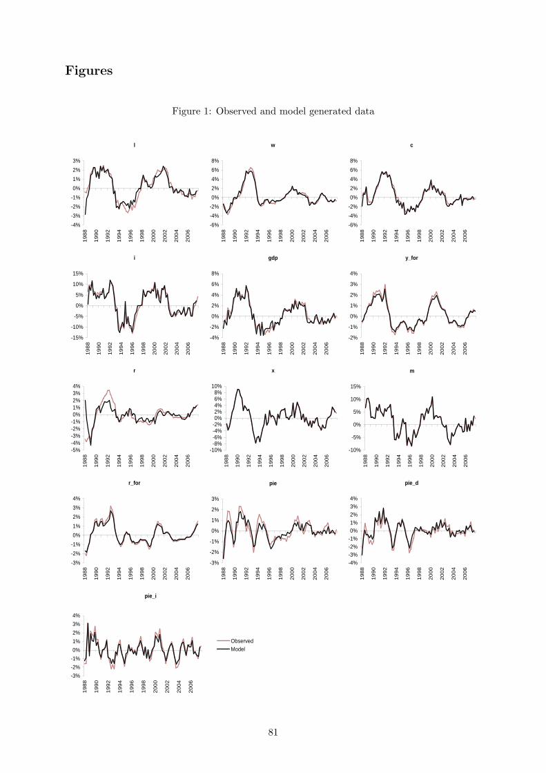
Figures
Figure 1: Observed and model generated data
pie_d
-4%-3%-2%-1%0%1%2%3%4%
19
88
19
90
19
92
19
94
19
96
19
98
20
00
20
02
20
04
20
06
w
-6%
-4%
-2%
0%
2%
4%
6%
8%
19
88
19
90
19
92
19
94
19
96
19
98
20
00
20
02
20
04
20
06
c
-6%
-4%
-2%
0%
2%
4%
6%
8%
19
88
19
90
19
92
19
94
19
96
19
98
20
00
20
02
20
04
20
06
i
-15%
-10%
-5%
0%
5%
10%
15%
19
88
19
90
19
92
19
94
19
96
19
98
20
00
20
02
20
04
20
06
r
-5%-4%-3%-2%-1%0%1%2%3%4%
19
88
19
90
19
92
19
94
19
96
19
98
20
00
20
02
20
04
20
06
l
-4%
-3%
-2%
-1%
0%
1%
2%
3%
19
88
19
90
19
92
19
94
19
96
19
98
20
00
20
02
20
04
20
06
gdp
-4%
-2%
0%
2%
4%
6%
8%
19
88
19
90
19
92
19
94
19
96
19
98
20
00
20
02
20
04
20
06
x
-10%-8%-6%-4%-2%0%2%4%6%8%
10%
19
88
19
90
19
92
19
94
19
96
19
98
20
00
20
02
20
04
20
06
m
-10%
-5%
0%
5%
10%
15%
19
88
19
90
19
92
19
94
19
96
19
98
20
00
20
02
20
04
20
06
r_for
-3%
-2%
-1%
0%
1%
2%
3%
4%
19
88
19
90
19
92
19
94
19
96
19
98
20
00
20
02
20
04
20
06
pie
-3%
-2%
-1%
0%
1%
2%
3%
19
88
19
90
19
92
19
94
19
96
19
98
20
00
20
02
20
04
20
06
pie_i
-3%
-2%
-1%
0%
1%
2%
3%
4%
19
88
19
90
19
92
19
94
19
96
19
98
20
00
20
02
20
04
20
06
ObservedModel
y_for
-2%
-1%
0%
1%
2%
3%
4%
19
88
19
90
19
92
19
94
19
96
19
98
20
00
20
02
20
04
20
06
81

Figure 2: Priors and posteriors of estimated parameters of estimated parameters
0 0.2 0.4 0.60
5
10
15
SE_eta_eps_i
0.2 0.4 0.60
50
100
SE_eta_eps_c
0.02 0.04 0.06 0.080
100
200
300
SE_eta_eps_phi
0.02 0.04 0.06 0.080
200
400
SE_eta_eps_a
0 0.2 0.4 0.60
5
10
15
20
SE_eta_eps_l
0 0.2 0.4 0.60
10
20
SE_eta_mu_d
0 0.2 0.4 0.60
20
40
SE_eta_mu_c
0 0.2 0.4 0.6 0.80
5
10SE_eta_mu_i
0 0.5 10
5
10SE_eta_mu_g
0 0.2 0.4 0.60
5
10
SE_eta_mu_x
0 0.2 0.4 0.60
10
20
30
SE_eta_mu_m
0.2 0.4 0.60
50
100
150
200
SE_eta_zeta
0.2 0.4 0.60
50
100
150
SE_eta_zeta_for
0 0.2 0.4 0.60
10
20
SE_eta_tau_l
0.02 0.04 0.06 0.080
200
400
600
SE_eta_tau_c
0.02 0.04 0.06 0.080
100
200
300
SE_eta_g
0.02 0.04 0.06 0.080
100
200
300
400
SE_eta_pie_for
0.02 0.04 0.06 0.080
500
1000
SE_eta_y_for
82
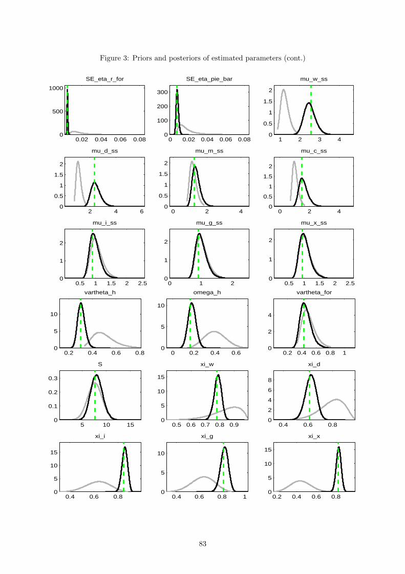
Figure 3: Priors and posteriors of estimated parameters (cont.)
0.02 0.04 0.06 0.080
500
1000
SE_eta_r_for
0 0.02 0.04 0.06 0.080
100
200
300
SE_eta_pie_bar
1 2 3 40
0.5
1
1.5
2
mu_w_ss
2 4 60
0.5
1
1.5
2
mu_d_ss
0 2 40
0.5
1
1.5
2
mu_m_ss
0 2 40
0.5
1
1.5
2
mu_c_ss
0.5 1 1.5 2 2.50
1
2
mu_i_ss
0 1 20
1
2
mu_g_ss
0.5 1 1.5 2 2.50
1
2
mu_x_ss
0.2 0.4 0.6 0.80
5
10
vartheta_h
0 0.2 0.4 0.60
5
10
omega_h
0.2 0.4 0.6 0.8 10
2
4
vartheta_for
5 10 150
0.1
0.2
0.3
S
0.5 0.6 0.7 0.8 0.90
5
10
15
xi_w
0.4 0.6 0.80
2
4
6
8
xi_d
0.4 0.6 0.80
5
10
15
xi_i
0.4 0.6 0.8 10
5
10
xi_g
0.2 0.4 0.6 0.80
5
10
15
xi_x
83
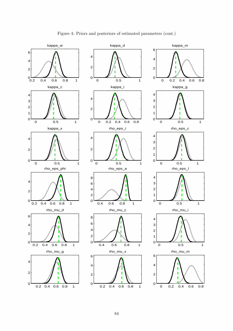
Figure 4: Priors and posteriors of estimated parameters (cont.)
0.2 0.4 0.6 0.8 10
2
4
6
kappa_w
0 0.5 10
2
4
kappa_d
0 0.2 0.4 0.6 0.80
2
4
6kappa_m
0 0.5 10
1
2
3
4
kappa_c
0 0.2 0.4 0.6 0.80
2
4
kappa_i
0 0.5 10
1
2
3
4
kappa_g
0 0.5 10
2
4
kappa_x
0 0.5 10
2
4
rho_eps_i
0 0.5 10
1
2
3
4
rho_eps_c
0.2 0.4 0.6 0.8 10
2
4
rho_eps_phi
0.4 0.6 0.8 10
2
4
6
8
rho_eps_a
0 0.5 10
1
2
3
4
rho_eps_l
0.2 0.4 0.6 0.8 10
2
4
6
rho_mu_d
0.4 0.6 0.8 10
2
4
6
8
rho_mu_c
0 0.5 10
1
2
3
4
rho_mu_i
0.2 0.4 0.6 0.8 10
2
4
rho_mu_g
0.2 0.4 0.6 0.8 10
2
4
6
rho_mu_x
0 0.2 0.4 0.6 0.80
2
4
6rho_mu_m
84
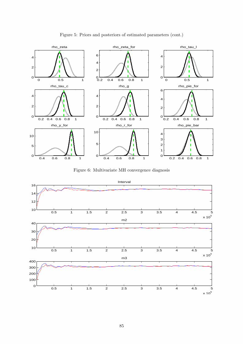
Figure 5: Priors and posteriors of estimated parameters (cont.)
0 0.5 10
2
4
rho_zeta
0.2 0.4 0.6 0.8 10
2
4
6
rho_zeta_for
0 0.5 10
2
4
rho_tau_l
0.2 0.4 0.6 0.8 10
2
4
rho_tau_c
0.2 0.4 0.6 0.8 10
2
4
rho_g
0.2 0.4 0.6 0.8 10
2
4
6rho_pie_for
0.4 0.6 0.8 10
5
10
rho_y_for
0.4 0.6 0.8 10
5
10
rho_r_for
0.2 0.4 0.6 0.8 10
1
2
3
4
rho_pie_bar
Figure 6: Multivariate MH convergence diagnosis
0.5 1 1.5 2 2.5 3 3.5 4 4.5 5
x 105
10
12
14
16Interval
0.5 1 1.5 2 2.5 3 3.5 4 4.5 5
x 105
10
20
30
40m2
0.5 1 1.5 2 2.5 3 3.5 4 4.5 5
x 105
0
100
200
300
400m3
85
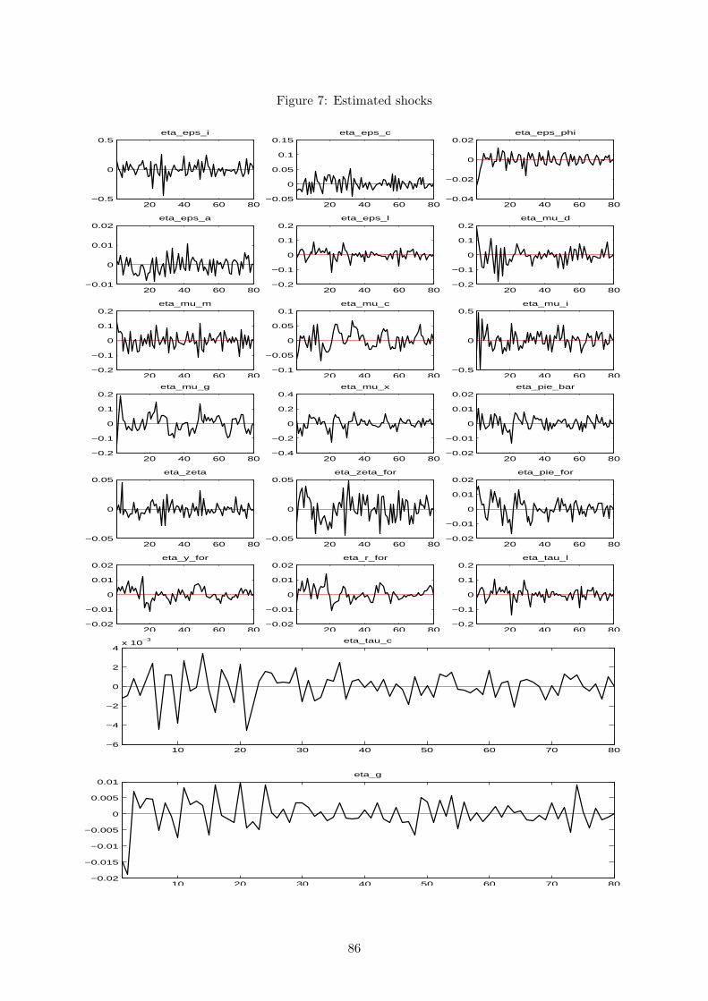
Figure 7: Estimated shocks
20 40 60 80−0.5
0
0.5eta_eps_i
20 40 60 80−0.05
0
0.05
0.1
0.15eta_eps_c
20 40 60 80−0.04
−0.02
0
0.02eta_eps_phi
20 40 60 80−0.01
0
0.01
0.02eta_eps_a
20 40 60 80−0.2
−0.1
0
0.1
0.2eta_eps_l
20 40 60 80−0.2
−0.1
0
0.1
0.2eta_mu_d
20 40 60 80−0.2
−0.1
0
0.1
0.2eta_mu_m
20 40 60 80−0.1
−0.05
0
0.05
0.1eta_mu_c
20 40 60 80−0.5
0
0.5eta_mu_i
20 40 60 80−0.2
−0.1
0
0.1
0.2eta_mu_g
20 40 60 80−0.4
−0.2
0
0.2
0.4eta_mu_x
20 40 60 80−0.02
−0.01
0
0.01
0.02eta_pie_bar
20 40 60 80−0.05
0
0.05eta_zeta
20 40 60 80−0.05
0
0.05eta_zeta_for
20 40 60 80−0.02
−0.01
0
0.01
0.02eta_pie_for
20 40 60 80−0.02
−0.01
0
0.01
0.02eta_y_for
20 40 60 80−0.02
−0.01
0
0.01
0.02eta_r_for
20 40 60 80−0.2
−0.1
0
0.1
0.2eta_tau_l
10 20 30 40 50 60 70 80−6
−4
−2
0
2
4x 10
−3 eta_tau_c
10 20 30 40 50 60 70 80−0.02
−0.015
−0.01
−0.005
0
0.005
0.01eta_g
86

Figure 8: Bayesian IRFs to a positive productivity shock
20 40 60 80 100
−2
−1
0
1
x 10−3 pie_d
20 40 60 80 100
−5
0
5
x 10−4 pie
20 40 60 80 100
−10
−5
0
5
x 10−5 pie_i
20 40 60 80 100
1
2
3
4
5
x 10−3 w
20 40 60 80 1000
5
10
x 10−3 c
20 40 60 80 1000
0.01
0.02
i
20 40 60 80 100
−4
−3
−2
−1
0
x 10−3 r
20 40 60 80 100−8
−6
−4
−2
0
2
x 10−3 l
20 40 60 80 1000
5
10
15
x 10−3 gdp
20 40 60 80 100
0
10
20
x 10−4 x
20 40 60 80 100
−1
0
1
2x 10
−3 m
87

Appendices
A Derivation of the model’s equations
We now present in detail the derivation of the model’s equations. For aspects not covered here
please refer to the main article, where (hopefully) they are explained.
A.1 Households
For the sake of exposition simplicity, we divide the household’s problem in two, analysing the
wage setting problem separately. The first part of the maximisation problem is given by:
maxCt(i),Bt+1(i),B∗t+1(i),It(i),Kt+1(i)
E0
∞∑
t=0
βt
{εct ln [Ct(i)− hCt−1(i)]− εl
t
1 + σlLt(i)1+σl
}
s.t.
(1− δ) Kt(i) + εit
[1− S
(It(i)
It−1(i)
)]It(i) = Kt+1(i) (135)
Rt−1Bt(i)Pt
+ R∗t−1Φ
(b∗t , ε
φt−1
) B∗t (i)Pt
+(1− τ l
t
) Wt(i)Pt
Lt(i) + At(i) + rkt Kt(i)+
+ trt + divt =Bt+1(i)
Pt+
B∗t+1(i)Pt
+ Ct(i) + pitIt(i) (136)
Forming the Lagrangian, LU1(i), we can rewrite the maximisation problem as:
maxCt(i),Bt+1(i),B∗t+1(i),It(i),Kt+1(i)
Lh1(i) = E0
∞∑
t=0
βt {εct ln [Ct(i)− hCt−1(i)]−
− εlt
1 + σlLt(i)1+σl + λu
t (i)[Rt−1
Bt(i)Pt
+ R∗t−1Φ
(b∗t , ε
φt−1
) B∗t (i)Pt
+(1− τ l
t
) Wt(i)Pt
Lt(i)+
+At(i) + rkt Kt(i) + trt + divt − Bt+1(i)
Pt− B∗
t+1(i)Pt
− Ct(i)− pitIt(i)
]+
+υUt (i)
[(1− δ) Kt(i) + εi
t
[1− S
(It(i)
It−1(i)
)]It(i)−Kt+1(i)
]}
where λut (i) is the lagrange multiplier associated with the budget constraint, which represents
the marginal utility of an additional unit of resources (wealth) available to consume, purchase
bonds or invest and υUt (i) is the lagrange multiplier associated with the capital accumulation
equation, which represents the marginal utility of an additional unit of resources available to
form another unit of capital stock.
88
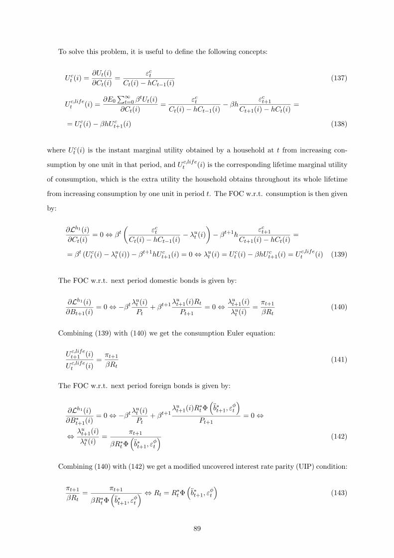
To solve this problem, it is useful to define the following concepts:
U ct (i) =
∂Ut(i)∂Ct(i)
=εct
Ct(i)− hCt−1(i)(137)
U c,lifet (i) =
∂E0∑∞
t=0 βtUt(i)∂Ct(i)
=εct
Ct(i)− hCt−1(i)− βh
εct+1
Ct+1(i)− hCt(i)=
= U ct (i)− βhU c
t+1(i) (138)
where U ct (i) is the instant marginal utility obtained by a household at t from increasing con-
sumption by one unit in that period, and U c,lifet (i) is the corresponding lifetime marginal utility
of consumption, which is the extra utility the household obtains throughout its whole lifetime
from increasing consumption by one unit in period t. The FOC w.r.t. consumption is then given
by:
∂Lh1(i)∂Ct(i)
= 0 ⇔ βt
(εct
Ct(i)− hCt−1(i)− λu
t (i))− βt+1h
εct+1
Ct+1(i)− hCt(i)=
= βt (U ct (i)− λu
t (i))− βt+1hU ct+1(i) = 0 ⇔ λu
t (i) = U ct (i)− βhU c
t+1(i) = U c,lifet (i) (139)
The FOC w.r.t. next period domestic bonds is given by:
∂Lh1(i)∂Bt+1(i)
= 0 ⇔ −βt λut (i)Pt
+ βt+1 λut+1(i)Rt
Pt+1= 0 ⇔ λu
t+1(i)λu
t (i)=
πt+1
βRt(140)
Combining (139) with (140) we get the consumption Euler equation:
U c,lifet+1 (i)
U c,lifet (i)
=πt+1
βRt(141)
The FOC w.r.t. next period foreign bonds is given by:
∂Lh1(i)∂B∗
t+1(i)= 0 ⇔ −βt λ
ut (i)Pt
+ βt+1λu
t+1(i)R∗t Φ
(b∗t+1, ε
φt
)
Pt+1= 0 ⇔
⇔ λut+1(i)λu
t (i)=
πt+1
βR∗t Φ
(b∗t+1, ε
φt
) (142)
Combining (140) with (142) we get a modified uncovered interest rate parity (UIP) condition:
πt+1
βRt=
πt+1
βR∗t Φ
(b∗t+1, ε
φt
) ⇔ Rt = R∗t Φ
(b∗t+1, ε
φt
)(143)
89

The FOC w.r.t. investment is given by:
∂Lh1(i)∂It(i)
= 0 ⇔ βt
{−pi
tλut (i) + υu
t (i)εit
[−S′
(It(i)
It−1(i)
)It(i)
It−1(i)+ 1− S
(It(i)
It−1(i)
)]}+
+ βt+1υut+1(i)ε
it+1It+1(i)S′
(It+1(i)It(i)
)It+1(i)It(i)
2 = 0 ⇔
⇔ −pitλ
ut (i)− υu
t (i)εit
[S′
(It(i)
It−1(i)
)It(i)
It−1(i)− 1 + S
(It(i)
It−1(i)
)]=
= −βυut+1(i)ε
it+1S
′(
It+1(i)It(i)
)(It+1(i)It(i)
)2
⇔
⇔ −pit −Qt(i)εi
t
[S′
(It(i)
It−1(i)
)It(i)
It−1(i)− 1 + S
(It(i)
It−1(i)
)]=
= −βQt+1(i)λu
t+1(i)λu
t (i)εit+1S
′(
It+1(i)It(i)
)(It+1(i)It(i)
)2
⇔
⇔ Qt(i)εit
[1− S
(It(i)
It−1(i)
)− S′
(It(i)
It−1(i)
)It(i)
It−1(i)
]+
+ βQt+1(i)λu
t+1(i)λu
t (i)εit+1S
′(
It+1(i)It(i)
)(It+1(i)It(i)
)2
= pit (144)
where Qt(i) = υut (i)
λut (i) is Tobin’s Q. Combining (140) with (144):
Qt(i)εit
[1− S
(It(i)
It−1(i)
)− S′
(It(i)
It−1(i)
)It(i)
It−1(i)
]+
+ Qt+1(i)πt+1
Rtεit+1S
′(
It+1(i)It(i)
)(It+1(i)It(i)
)2
= pit (145)
The FOC w.r.t. the capital stock is given by:
∂Lh1(i)∂Kt+1
= 0 ⇔ −βtυut (i) + βt+1
(λu
t+1(i)rkt+1 + υu
t+1(i) (1− δ))
= 0 ⇔ υut (i) =
= β(λu
t+1(i)rkt+1 + υu
t+1(i) (1− δ))⇔ Qt(i) = β
λut+1(i)λu
t (i)
(rkt+1 + Qt+1(i) (1− δ)
)(146)
Combining (140) with (146):
Qt(i) =πt+1
Rt
(rkt+1 + Qt+1(i) (1− δ)
)(147)
We now turn to the wage setting problem, where we suppress all terms and constraints that
are not relevant for this decision, for the sake of exposition simplicity. Furthermore, we denote
individual variables, related with the wage/labour decision, with a ”˜”, to reinforce that this
problem only concerns households who get to reoptimise in t. To solve this problem, it is useful
to define U lt(i), the instant marginal utility obtained by a household that gets to increase its
90
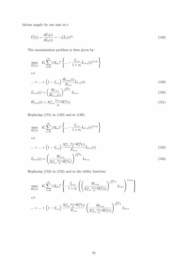
labour supply by one unit in t:
U lt(i) =
∂Ut(i)∂Lt(i)
= −εltLt(i)σl (148)
The maximisation problem is then given by:
maxW 0
t (i)Et
∞∑
s=0
(βξw)s
{...− εl
t+s
1 + σlLt+s(i)1+σl
}
s.t.
... = ... +(1− τ l
t+s
) Wt+s(i)Pt+s
Lt+s(i) (149)
Lt+s(i) =(
Wt+s
Wt+s(i)
) µwµw−1
Lt+s (150)
Wt+s(i) = Xwt+s
zt+s
ztW 0
t (i) (151)
Replacing (151) in (150) and in (149):
maxW 0
t (i)Et
∞∑
s=0
(βξw)s
{...− εl
t+s
1 + σlLt+s(i)1+σl
}
s.t.
... = ... +(1− τ l
t+s
) Xwt+s
zt+s
ztW 0
t (i)Pt+s
Lt+s(i) (152)
Lt+s(i) =
(Wt+s
Xwt+s
zt+s
ztW 0
t (i)
) µwµw−1
Lt+s (153)
Replacing (153) in (152) and in the utility function:
maxW 0
t (i)Et
∞∑
s=0
(βξw)s
−
εlt+s
1 + σl
(Wt+s
Xwt+s
zt+s
ztW 0
t (i)
) µwµw−1
Lt+s
1+σl
s.t.
... = ... +(1− τ l
t+s
) Xwt+s
zt+s
ztW 0
t (i)Pt+s
(Wt+s
Xwt+s
zt+s
ztW 0
t (i)
) µwµw−1
Lt+s
91
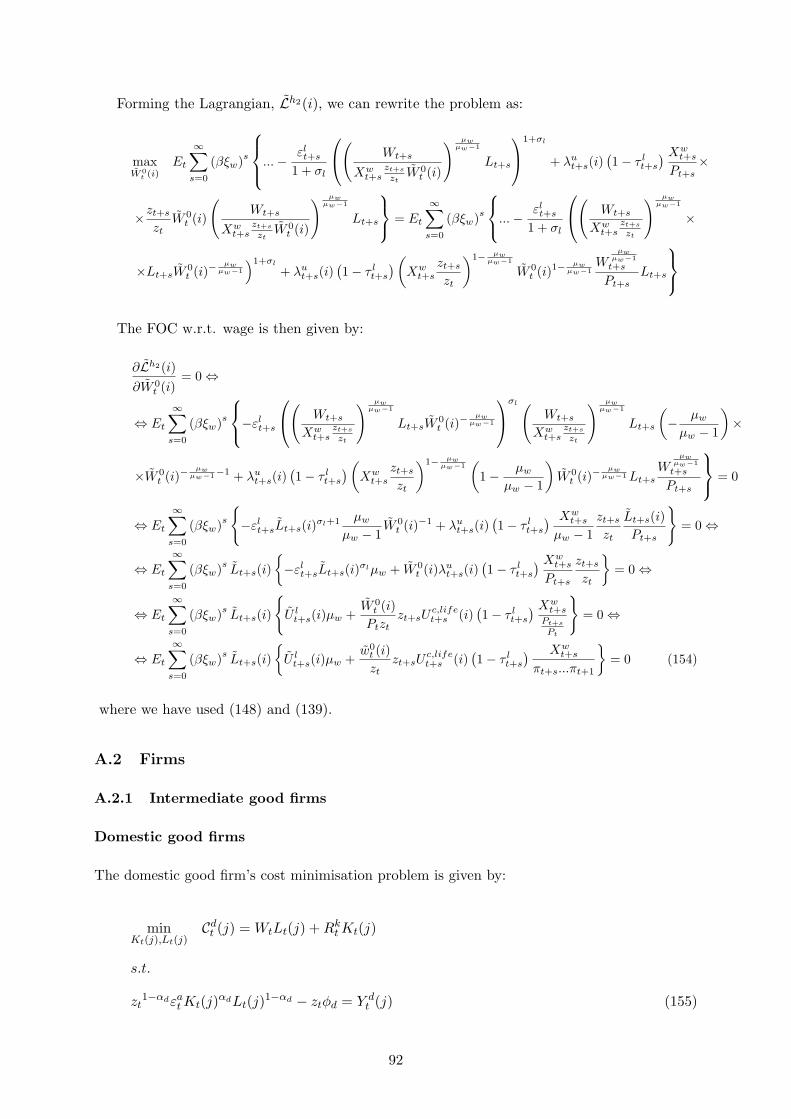
Forming the Lagrangian, Lh2(i), we can rewrite the problem as:
maxW 0
t (i)Et
∞∑s=0
(βξw)s
...− εlt+s
1 + σl
(Wt+s
Xwt+s
zt+s
ztW 0
t (i)
) µwµw−1
Lt+s
1+σl
+ λut+s(i)
(1− τ l
t+s
) Xwt+s
Pt+s×
×zt+s
ztW 0
t (i)
(Wt+s
Xwt+s
zt+s
ztW 0
t (i)
) µwµw−1
Lt+s
= Et
∞∑s=0
(βξw)s
...− εl
t+s
1 + σl
(Wt+s
Xwt+s
zt+s
zt
) µwµw−1
×
×Lt+sW0t (i)−
µwµw−1
)1+σl
+ λut+s(i)
(1− τ l
t+s
)(Xw
t+s
zt+s
zt
)1− µwµw−1
W 0t (i)1−
µwµw−1
Wµw
µw−1t+s
Pt+sLt+s
The FOC w.r.t. wage is then given by:
∂Lh2(i)∂W 0
t (i)= 0 ⇔
⇔ Et
∞∑s=0
(βξw)s
−εl
t+s
(Wt+s
Xwt+s
zt+s
zt
) µwµw−1
Lt+sW0t (i)−
µwµw−1
σl (Wt+s
Xwt+s
zt+s
zt
) µwµw−1
Lt+s
(− µw
µw − 1
)×
×W 0t (i)−
µwµw−1−1 + λu
t+s(i)(1− τ l
t+s
) (Xw
t+s
zt+s
zt
)1− µwµw−1
(1− µw
µw − 1
)W 0
t (i)−µw
µw−1 Lt+sW
µwµw−1
t+s
Pt+s
= 0
⇔ Et
∞∑s=0
(βξw)s
{−εl
t+sLt+s(i)σl+1 µw
µw − 1W 0
t (i)−1 + λut+s(i)
(1− τ l
t+s
) Xwt+s
µw − 1zt+s
zt
Lt+s(i)Pt+s
}= 0 ⇔
⇔ Et
∞∑s=0
(βξw)sLt+s(i)
{−εl
t+sLt+s(i)σlµw + W 0t (i)λu
t+s(i)(1− τ l
t+s
) Xwt+s
Pt+s
zt+s
zt
}= 0 ⇔
⇔ Et
∞∑s=0
(βξw)sLt+s(i)
{U l
t+s(i)µw +W 0
t (i)Ptzt
zt+sUc,lifet+s (i)
(1− τ l
t+s
) Xwt+s
Pt+s
Pt
}= 0 ⇔
⇔ Et
∞∑s=0
(βξw)sLt+s(i)
{U l
t+s(i)µw +w0
t (i)zt
zt+sUc,lifet+s (i)
(1− τ l
t+s
) Xwt+s
πt+s...πt+1
}= 0 (154)
where we have used (148) and (139).
A.2 Firms
A.2.1 Intermediate good firms
Domestic good firms
The domestic good firm’s cost minimisation problem is given by:
minKt(j),Lt(j)
Cdt (j) = WtLt(j) + Rk
t Kt(j)
s.t.
zt1−αdεa
t Kt(j)αdLt(j)1−αd − ztφd = Y dt (j) (155)
92
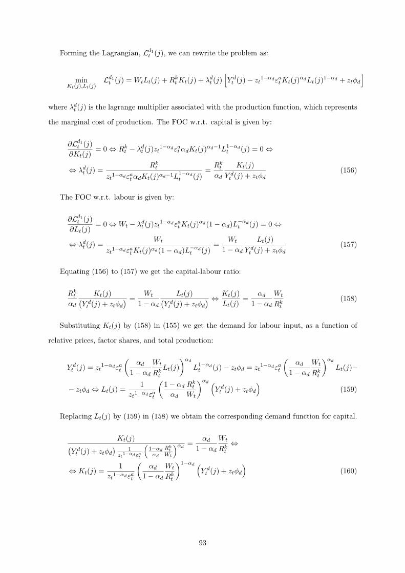
Forming the Lagrangian, Ld1t (j), we can rewrite the problem as:
minKt(j),Lt(j)
Ld1t (j) = WtLt(j) + Rk
t Kt(j) + λdt (j)
[Y d
t (j)− zt1−αdεa
t Kt(j)αdLt(j)1−αd + ztφd
]
where λdt (j) is the lagrange multiplier associated with the production function, which represents
the marginal cost of production. The FOC w.r.t. capital is given by:
∂Ld1t (j)
∂Kt(j)= 0 ⇔ Rk
t − λdt (j)zt
1−αdεat αdKt(j)αd−1L1−αd
t (j) = 0 ⇔
⇔ λdt (j) =
Rkt
zt1−αdεa
t αdKt(j)αd−1L1−αdt (j)
=Rk
t
αd
Kt(j)Y d
t (j) + ztφd(156)
The FOC w.r.t. labour is given by:
∂Ld1t (j)
∂Lt(j)= 0 ⇔ Wt − λd
t (j)zt1−αdεa
t Kt(j)αd(1− αd)L−αdt (j) = 0 ⇔
⇔ λdt (j) =
Wt
zt1−αdεa
t Kt(j)αd(1− αd)L−αdt (j)
=Wt
1− αd
Lt(j)Y d
t (j) + ztφd(157)
Equating (156) to (157) we get the capital-labour ratio:
Rkt
αd
Kt(j)(Y d
t (j) + ztφd
) =Wt
1− αd
Lt(j)(Y d
t (j) + ztφd
) ⇔ Kt(j)Lt(j)
=αd
1− αd
Wt
Rkt
(158)
Substituting Kt(j) by (158) in (155) we get the demand for labour input, as a function of
relative prices, factor shares, and total production:
Y dt (j) = zt
1−αdεat
(αd
1− αd
Wt
Rkt
Lt(j))αd
L1−αdt (j)− ztφd = zt
1−αdεat
(αd
1− αd
Wt
Rkt
)αd
Lt(j)−
− ztφd ⇔ Lt(j) =1
zt1−αdεa
t
(1− αd
αd
Rkt
Wt
)αd (Y d
t (j) + ztφd
)(159)
Replacing Lt(j) by (159) in (158) we obtain the corresponding demand function for capital.
Kt(j)(Y d
t (j) + ztφd
)1
zt1−αdεa
t
(1−αd
αd
Rkt
Wt
)αd=
αd
1− αd
Wt
Rkt
⇔
⇔ Kt(j) =1
zt1−αdεa
t
(αd
1− αd
Wt
Rkt
)1−αd (Y d
t (j) + ztφd
)(160)
93
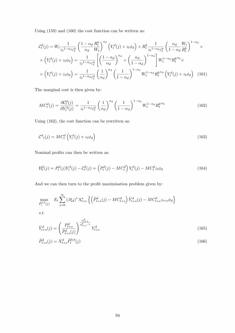
Using (159) and (160) the cost function can be written as:
Cdt (j) = Wt
1zt
1−αdεat
(1− αd
αd
Rkt
Wt
)αd (Y d
t (j) + ztφd
)+ Rk
t
1zt
1−αdεat
(αd
1− αd
Wt
Rkt
)1−αd
×
×(Y d
t (j) + ztφd
)=
1zt
1−αdεat
[(1− αd
αd
)αd
+(
αd
1− αd
)1−αd]
W 1−αdt Rk
tαd×
×(Y d
t (j) + ztφd
)=
1zt
1−αdεat
(1αd
)αd(
11− αd
)1−αd
W 1−αdt Rk
tαd
(Y d
t (j) + ztφd
)(161)
The marginal cost is then given by:
MCdt (j) =
∂Cdt (j)
∂Y dt (j)
=1
zt1−αdεa
t
(1αd
)αd(
11− αd
)1−αd
W 1−αdt Rk
tαd (162)
Using (162), the cost function can be rewritten as:
Cdt(j) = MCd
t
(Y d
t (j) + ztφd
)(163)
Nominal profits can then be written as:
Πdt (j) = P d
t (j)Y dt (j)− Cd
t (j) =(P d
t (j)−MCdt
)Y d
t (j)−MCdt ztφd (164)
And we can then turn to the profit maximisation problem given by:
maxP 0,d
t (j)Et
∞∑
s=0
(βξd)s Λu
t+s
{(P d
t+s(j)−MCdt+s
)Y d
t+s(j)−MCdt+szt+sφd
}
s.t.
Y dt+s(j) =
(P d
t+s
P dt+s(j)
) µdt+s
µdt+s−1
Y dt+s (165)
P dt+s(j) = Xd
t+sP0,dt (j) (166)
94
where Λut+s =
λut+s
Pt+s. Replacing (166) in (165) and in the profit function:
maxP 0,d
t (j)Et
∞∑
s=0
(βξd)s Λu
t+s
{(Xd
t+sP0,dt (j)−MCd
t+s
)Y d
t+s(j)−MCdt+szt+sφd
}
s.t.
Y dt+s(j) =
(P d
t+s
Xdt+sP
0,dt (j)
) µdt+s
µdt+s−1
Y dt+s (167)
Replacing (167) in the profit function:
maxP 0,d
t (j)Ld2
t (j) = Et
∞∑
s=0
(βξd)s Λu
t+s
(Xd
t+sP0,dt (j)−MCd
t+s
) (P d
t+s
Xdt+sP
0,dt (j)
) µdt+s
µdt+s−1
Y dt+s−
−MCdt+szt+sφd
}= Et
∞∑
s=0
(βξd)s Λu
t+s
(Xd
t+sP0,dt (j)
)1− µdt+s
µdt+s−1
(P d
t+s
) µdt+s
µdt+s−1 Y d
t+s−
−MCdt+s
(P d
t+s
Xdt+sP
0,dt (j)
) µdt+s
µdt+s−1
Y dt+s −MCd
t+szt+sφd
The FOC w.r.t. the price of the domestic good is then given by:
∂Ld2t (j)
∂P 0,dt (j)
= 0 ⇔
⇔ Et
∞∑
s=0
(βξd)s Λu
t+s
(1− µd
t+s
µdt+s − 1
)(Xd
t+sP0,dt (j)
)− µdt+s
µdt+s−1 Xd
t+s
(P d
t+s
) µdt+s
µdt+s−1 Y d
t+s−
−MCdt+s
(µd
t+s
µdt+s − 1
)(P d
t+s
Xdt+sP
0,dt (j)
) µdt+s
µdt+s−1
−1P d
t+s
Xdt+s
(− 1
P 0,dt (j)2
)Y d
t+s
= 0 ⇔
⇔ Et
∞∑
s=0
(βξd)s Λu
t+s
{(1− µd
t+s
µdt+s − 1
)Xd
t+sYdt+s(j) + MCd
t+s
(µd
t+s
µdt+s − 1
)Y d
t+s(j)
P 0,dt (j)
}= 0
⇔ Et
∞∑
s=0
(βξd)s Λu
t+s
µdt+s − 1
Y dt+s(j)
{Xd
t+sP0,dt (j)−MCd
t+sµdt+s
}= 0 ⇔
⇔ Et
∞∑
s=0
(βξd)s Λu
t+s
µdt+s − 1
Y dt+s(j)P
dt+s
Xdt+s
P dt+s
P dt
P 0,dt (j)Pt
P dt
Pt
−MCd
t+s
Pt+s
P dt+s
Pt+s
µdt+s
= 0 ⇔
⇔ Et
∞∑
s=0
(βξd)s λu
t+s
µdt+s − 1
Y dt+s(j)p
dt+s
{Xd
t+s
πdt+s...π
dt+1
p0,dt (j)pd
t
− mcdt+s
pdt+s
µdt+s
}= 0 (168)
95

Import good firms
Following the same reasonings applied to domestic good firms, nominal profits of the represen-
tative import good firm can be written as:
Πmt (m) = (Pm
t (m)−MCmt ) Y m
t (m)−MCmt ztφm (169)
where:
MCmt+s = P ∗
t+s (170)
The corresponding profit maximisation problem is then given by:
maxP 0,m
t (m)Et
∞∑
s=0
(βξm)s Λut+s
{(Pm
t+s(m)−MCmt+s
)Y m
t+s(m)−MCmt+szt+sφm
}
s.t.
Y mt+s(m) =
(Pm
t+s
Pmt+s(m)
) µmt+s
µmt+s−1
Y mt+s (171)
Pmt+s(m) = Xm
t+sP0,mt (m) (172)
Which produces the following FOC w.r.t. the price of import good:
Et
∞∑
s=0
(βξm)s λut+s
µmt+s − 1
Y mt+s(m)pm
t+s
{Xm
t+s
πmt+s...π
mt+1
p0,mt (m)pm
t
− mcmt+s
pmt+s
µmt+s
}= 0 (173)
Composite good firm
The composite good firm’s cost minimisation problem is given by:
minY d
t ,Y mt
Cct = P d
t Y dt + Pm
t Y mt
s.t.
[(1− ωh)
1ϑh+1 Y d
t
ϑhϑh+1 + ω
1ϑh+1
h Y mt
ϑhϑh+1
]ϑh+1
ϑh
= Y ht (174)
96
Forming the Lagrangian, Lct , we can rewrite the problem as:
minY d
t ,Y mt
Lct = P d
t Y dt + Pm
t Y mt + λc
t
[(1− ωh)
1ϑh+1 Y d
t
ϑhϑh+1 + ω
1ϑh+1
h Y mt
ϑhϑh+1
]ϑh+1
ϑh
where λct is the lagrange multiplier associated with the production function, which represents
the marginal cost of production. Analogously to the domestic good firm case, we obtain the
following three equations. The FOC w.r.t. domestic good:
Y dt = (1− ωh)
(P h
t
P dt
)ϑh+1
Y ht (175)
The FOC w.r.t. import good:
Y mt = ωh
(P h
t
Pmt
)ϑh+1
Y ht (176)
A.2.2 Final good firms
Following the same reasonings applied to domestic and import good firms, nominal profits of
the representative type f final good firm can be written as:
Πft (n) =
(P f
t (n)−MCft
)Y f
t (n)−MCft ztφf (177)
where:
MCft+s = P h
t+s (178)
The corresponding profit maximisation problem is then given by:
maxP 0,f
t (n)Et
∞∑
s=0
(βξf )s Λut+s
{(P f
t+s(n)−MCft+s
)Y f
t+s(n)−MCft+szt+sφf
}
s.t.
Y ft+s(n) =
(P f
t+s
P ft+s(n)
) µft+s
µft+s−1
Y ft+s (179)
P ft+s(n) = Xf
t+sP0,ft (n) (180)
97
Which produces the following FOC w.r.t. the price of final good:
Et
∞∑
s=0
(βξf )s λut+s
µft+s − 1
Y ft+s(n)pf
t+s
{Xf
t+s
πft+s...π
ft+1
p0,ft (n)
pft
− mcft+s
pft+s
µft+s
}= 0 (181)
A.3 Aggregators
The labour aggregator’s cost minimisation problem is given by:
minLt(i)
Clt =
∫ 1
0Wt(i)Lt(i)di
s.t.(∫ 1
0Lt(i)
1µw di
)µw
= Lt (182)
Forming the Lagrangian, Llt, we can rewrite the problem as:
minLt(i)
Llt =
∫ 1
0Wt(i)Lt(i)di + λl
t
[Lt −
(∫ 1
0Lt(i)
1µw di
)µw]
where λlt is the lagrange multiplier associated with the production function, which corresponds
to the aggregator’s marginal cost. The FOC w.r.t. each variety of labour is then given by:
∂Llt
∂Lt(i)= 0 ⇔ Wt(i) + λl
t
[−µw
(∫ 1
0Lt(i)
1µw di
)µw−1 1µw
(Lt(i)
1µw−1
)]= 0 ⇔ Wt(i) =
= λlt
[L
µw−1µw
t Lt(i)−µw−1
µw
]⇔ Wt(i) = λl
t
(Lt
Lt(i)
)µw−1µw ⇔ Lt(i) =
(Wt
Wt(i)
) µwµw−1
Lt (183)
where we have used the fact that since the aggregator operates in perfect competition, we can
replace its marginal cost by the wage it charges.
All the other aggregators solve a perfectly analogous problem to the one solved by the labour
aggregator. In the case of the domestic good aggregator, the problem is described by:
minY d
t (j)Cd
t =∫ 1
0P d
t (j)Y dt (j)dj
s.t.
(∫ 1
0Y d
t (j)1
µdt dj
)µdt
= Y dt (184)
98
and the FOC is given by:
Y dt (j) =
(P d
t
P dt (j)
) µdt
µdt−1
Y dt (185)
In the case of the import good aggregator, the problem is described by:
minY m
t (m)Cm
t =∫ 1
0Pm
t (m)Y mt (m)dm
s.t.
(∫ 1
0Y m
t (m)1
µmt dm
)µmt
= Y mt (186)
and the FOC is given by:
Y mt (m) =
(Pm
t
Pmt (m)
) µmt
µmt −1
Y mt (187)
And finally, in the case of type f final good aggregator, the problem is described by:
minY f
t (n)Cf
t =∫ 1
0P f
t (n)Y ft (n)dn
s.t.
(∫ 1
0Y f
t (n)1
µft dn
)µft
= Y ft (188)
and the FOC is given by:
Y ft (n) =
(P f
t
P ft (n)
) µft
µft −1
Y ft (189)
A.4 Rest of the world
The RW’s demand for export good, i.e. domestic exports, is exogenously given as:
Xt =(
P ∗t
Pt
)ϑ∗+1
Y ∗t (190)
99
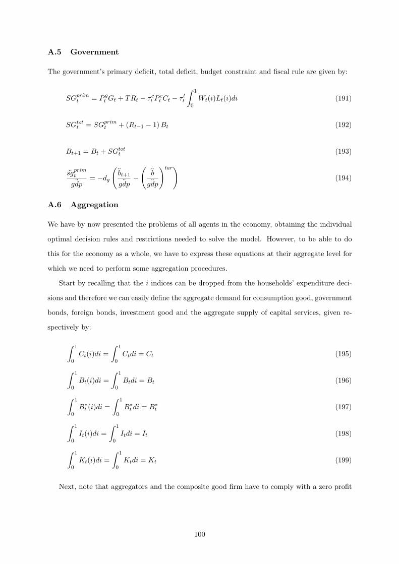
A.5 Government
The government’s primary deficit, total deficit, budget constraint and fiscal rule are given by:
SGprimt = P g
t Gt + TRt − τ ct P c
t Ct − τ lt
∫ 1
0Wt(i)Lt(i)di (191)
SGtott = SGprim
t + (Rt−1 − 1)Bt (192)
Bt+1 = Bt + SGtott (193)
sgprimt
¨gdp= −dg
(bt+1
¨gdp−
(b¨gdp
)tar)(194)
A.6 Aggregation
We have by now presented the problems of all agents in the economy, obtaining the individual
optimal decision rules and restrictions needed to solve the model. However, to be able to do
this for the economy as a whole, we have to express these equations at their aggregate level for
which we need to perform some aggregation procedures.
Start by recalling that the i indices can be dropped from the households’ expenditure deci-
sions and therefore we can easily define the aggregate demand for consumption good, government
bonds, foreign bonds, investment good and the aggregate supply of capital services, given re-
spectively by:
∫ 1
0Ct(i)di =
∫ 1
0Ctdi = Ct (195)
∫ 1
0Bt(i)di =
∫ 1
0Btdi = Bt (196)
∫ 1
0B∗
t (i)di =∫ 1
0B∗
t di = B∗t (197)
∫ 1
0It(i)di =
∫ 1
0Itdi = It (198)
∫ 1
0Kt(i)di =
∫ 1
0Ktdi = Kt (199)
Next, note that aggregators and the composite good firm have to comply with a zero profit
100

condition, as they work in perfect competition, and therefore the following equations hold:
WtLt −∫ 1
0Wt(i)Lt(i)di = 0 ⇔ WtLt =
∫ 1
0Wt(i)Lt(i)di (200)
P dt Y d
t −∫ 1
0P d
t (j)Y dt (j)dj = 0 ⇔ P d
t Y dt =
∫ 1
0P d
t (j)Y dt (j)dj (201)
Pmt Y m
t −∫ 1
0Pm
t (m)Y mt (m)dm = 0 ⇔ Pm
t Y mt =
∫ 1
0Pm
t (m)Y mt (m)dm (202)
P ft Y f
t −∫ 1
0P f
t (n)Y ft (n)df = 0 ⇔ P f
t Y ft =
∫ 1
0P f
t (n)Y ft (n)df (203)
P ht Y h
t − P dt Y d
t − Pmt Y m
t = 0 ⇔ P ht Y h
t = P dt Y d
t + Pmt Y m
t (204)
In addition, note that firms’ aggregate profits are given by:
∫ 1
0Πd
t (j)dj =∫ 1
0P d
t (j)Y dt (j)dj −Wt
∫ 1
0Lt(j)dj −Rk
t
∫ 1
0Kt(j)dj (205)
∫ 1
0Πm
t (m)dm =∫ 1
0P d
t (m)Y mt (m)dm− P ∗
t Mt (206)
∑
f
∫ 1
0Πf
t (n)df =∑
f
∫ 1
0P f
t (n)Y ft (n)df − P h
t
∑
f
Y ft (207)
Using (201)-(207), (227) and (228) we can write the following expression for aggregate profits
from firms, which must be equal to aggregate dividends received from households:
DIVt =∫ 1
0Πd
t (j)dj +∫ 1
0Πm
t (m)dm +∑
f
∫ 1
0Πt(n)df =
∫ 1
0P d
t (j)Y dt (j)dj −WtLt−
−Rkt Kt +
∫ 1
0P d
t (m)Y mt (m)dm− P ∗
t Mt +∑
f
∫ 1
0P f
t (n)Y ft (n)df − P h
t
∑
f
Y ft =
= P dt Y d
t −WtLt −Rkt Kt + Pm
t Y mt − P ∗
t Mt +∑
f
P ft Y f
t − P ht
∑
f
Y ft =
= P dt Y d
t −WtLt −Rkt Kt + P h
t Y ht − P d
t Y dt − P ∗
t Mt +∑
f
P ft Y f
t − P ht
∑
f
Y ft =
= −WtLt −Rkt Kt − P ∗
t Mt +∑
f
P ft Y f
t + P ht Y h
t − P ht
∑
f
Y ft (208)
Using (191), (192), (193) and (200) we then get the following expression for the government
101
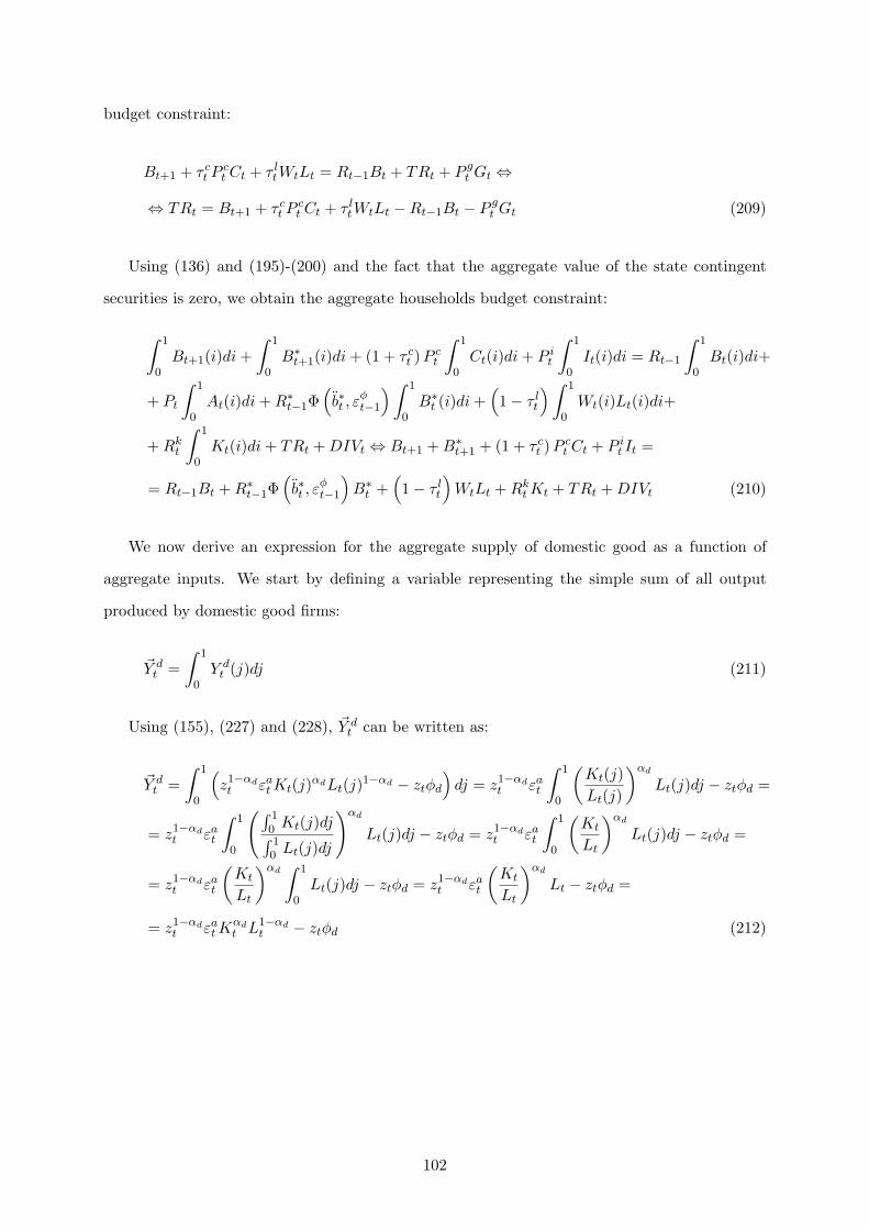
budget constraint:
Bt+1 + τ ct P c
t Ct + τ ltWtLt = Rt−1Bt + TRt + P g
t Gt ⇔
⇔ TRt = Bt+1 + τ ct P c
t Ct + τ ltWtLt −Rt−1Bt − P g
t Gt (209)
Using (136) and (195)-(200) and the fact that the aggregate value of the state contingent
securities is zero, we obtain the aggregate households budget constraint:
∫ 1
0Bt+1(i)di +
∫ 1
0B∗
t+1(i)di + (1 + τ ct ) P c
t
∫ 1
0Ct(i)di + P i
t
∫ 1
0It(i)di = Rt−1
∫ 1
0Bt(i)di+
+ Pt
∫ 1
0At(i)di + R∗
t−1Φ(b∗t , ε
φt−1
)∫ 1
0B∗
t (i)di +(1− τ l
t
)∫ 1
0Wt(i)Lt(i)di+
+ Rkt
∫ 1
0Kt(i)di + TRt + DIVt ⇔ Bt+1 + B∗
t+1 + (1 + τ ct ) P c
t Ct + P it It =
= Rt−1Bt + R∗t−1Φ
(b∗t , ε
φt−1
)B∗
t +(1− τ l
t
)WtLt + Rk
t Kt + TRt + DIVt (210)
We now derive an expression for the aggregate supply of domestic good as a function of
aggregate inputs. We start by defining a variable representing the simple sum of all output
produced by domestic good firms:
~Y dt =
∫ 1
0Y d
t (j)dj (211)
Using (155), (227) and (228), ~Y dt can be written as:
~Y dt =
∫ 1
0
(z1−αdt εa
t Kt(j)αdLt(j)1−αd − ztφd
)dj = z1−αd
t εat
∫ 1
0
(Kt(j)Lt(j)
)αd
Lt(j)dj − ztφd =
= z1−αdt εa
t
∫ 1
0
(∫ 10 Kt(j)dj∫ 10 Lt(j)dj
)αd
Lt(j)dj − ztφd = z1−αdt εa
t
∫ 1
0
(Kt
Lt
)αd
Lt(j)dj − ztφd =
= z1−αdt εa
t
(Kt
Lt
)αd∫ 1
0Lt(j)dj − ztφd = z1−αd
t εat
(Kt
Lt
)αd
Lt − ztφd =
= z1−αdt εa
t Kαdt L1−αd
t − ztφd (212)
102

Furthermore, replacing Y dt (j) in (211) by (185):
~Y dt =
∫ 1
0
(P d
t
P dt (j)
) µdt
µdt−1
Y dt dj = Y d
t P dt
µdt
µdt−1
∫ 1
0P d
t (j)− µd
tµd
t−1 dj =
= Y dt P d
t
µdt
µdt−1
(~P d
t
)− µdt
µdt−1 ⇔ Y d
t =
(~P d
t
P dt
) µdt
µdt−1
~Y dt (213)
where:
~P dt =
(∫ 1
0P d
t (j)− µd
tµd
t−1 dj
)−µdt−1
µdt
(214)
We now want to derive the economy’s aggregate wage. We start by replacing (183) in (182):
Lt =
∫ 1
0
((Wt
Wt(i)
) µwµw−1
Lt
) 1µw
di
µw
=
(W
1µw−1
t L1
µwt
∫ 1
0
(1
Wt(i)
) 1µw−1
di
)µw
=
= Wµw
µw−1
t Lt
(∫ 1
0
(1
Wt(i)
) 1µw−1
di
)µw
⇔ Wt =(∫ 1
0Wt(i)
− 1µw−1 di
)−(µw−1)
(215)
Next, note that we can write:
W− 1
µw−1
t =∫ 1
0Wt(i)
− 1µw−1 di =
=∫
optimising housWt(i)
− 1µw−1 di +
∫
non optimising housWt(i)
− 1µw−1 di (216)
Concerning households that get to reoptimise, remember that they will all choose the same
wage, W 0t , and that each period there are (1− ξw) households that reoptimise. Therefore:
∫
optimising housWt(i)
− 1µw−1 di = (1− ξw)
(W 0
t
)− 1µw−1 (217)
As for households that do not reoptimise, things are a bit more complicated. There are
multiple different wages coming from t − 1 that we have to consider, with each one having
a density function associated. Furthermore, only a fraction of households that charged each
wage in the previous period won’t get to reoptimise. Consider that the different wages that
existed in t− 1 are indexed by ω. Wages that are not optimised in t are updated with previous
period inflation, according to the non-reoptimised wage rule. If we add over all possible wages
weighting by the number of households that posted that wage in t − 1 and won’t reoptimise it
in t, recalling that for household i that does not reoptimise in t, the wage is given by Wt(i) =
103

πκwt−1π
1−κwt ζtWt−1(i):
∫
non optimising hous
Wt(i)−1
µw−1 di =∫
ft−1,t(ω)(πκw
t−1π1−κwt ζtWt−1(ω)
)− 1µw−1 dω (218)
where ft−1,t(ω) is the ”number” of households that had wage Wt−1(ω) in t − 1 and were not
able to reoptimise in t. In principle, this integral is quite hard to evaluate. However, by the
Calvo randomisation assumption, we know that among all the firms who had Wt−1(ω) in t− 1
there is a constant percentage ξw who will not reoptimise in t and therefore, we can write:
ft−1,t(ω) = ξwft−1(ω) ∀ ω (219)
where ft−1(ω) is the total number of firms that had wage Wt−1(ω) in t− 1. Substituting (219)
in (218):
∫
non optimising housWt(i)
− 1µw−1 di =
= ξw
(πκw
t−1π1−κwt ζt
)− 1µw−1
∫ft−1(ω)Wt−1(ω)−
1µw−1 dω (220)
Now compare this expression with (216). The term∫
ft−1(ω)Wt−1(ω)−1
µw−1 dω is exactly
equivalent to (216) in period t − 1. In both cases, we are simply adding over all prices that
existed in the economy in t− 1. Therefore, we can rewrite (220) as:
∫
non optimising housWt(i)
− 1µw−1 di = ξw
(πκw
t−1π1−κwt ζt
)− 1µw−1 W
− 1µw−1
t−1 (221)
Substituting (217) and (221) in (215) we finally get the following expression for the average
aggregate wage index:
Wt =[(1− ξw)
(W 0
t
)− 1µw−1 + ξw
(πκw
t−1π1−κwt ζtWt−1
)− 1µw−1
]−(µw−1)
(222)
Using a perfectly analogous reasoning to the one developed above, we obtain similar equations
for the aggregate prices of domestic good, import good and type f final good:
P dt =
[(1− ξd)
(P 0,d
t
)− 1
µdt−1 + ξd
((πd
t−1
)κd
(πt)1−κd P d
t−1
)− 1
µdt−1
]−(µdt−1)
(223)
104
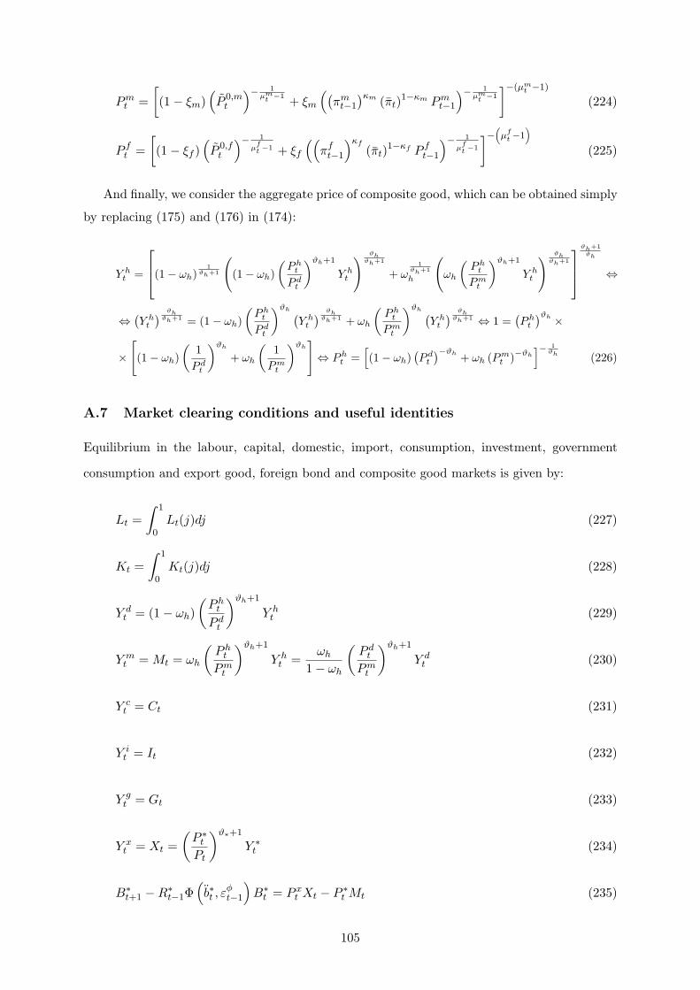
Pmt =
[(1− ξm)
(P 0,m
t
)− 1µm
t −1 + ξm
((πm
t−1
)κm (πt)1−κm Pm
t−1
)− 1µm
t −1
]−(µmt −1)
(224)
P ft =
[(1− ξf )
(P 0,f
t
)− 1
µft −1 + ξf
((πf
t−1
)κf
(πt)1−κf P f
t−1
)− 1
µft −1
]−(µf
t−1)
(225)
And finally, we consider the aggregate price of composite good, which can be obtained simply
by replacing (175) and (176) in (174):
Y ht =
(1− ωh)
1ϑh+1
((1− ωh)
(Ph
t
P dt
)ϑh+1
Y ht
) ϑhϑh+1
+ ω1
ϑh+1
h
(ωh
(Ph
t
Pmt
)ϑh+1
Y ht
) ϑhϑh+1
ϑh+1ϑh
⇔
⇔ (Y h
t
) ϑhϑh+1 = (1− ωh)
(Ph
t
P dt
)ϑh (Y h
t
) ϑhϑh+1 + ωh
(Ph
t
Pmt
)ϑh (Y h
t
) ϑhϑh+1 ⇔ 1 =
(Ph
t
)ϑh ×
×[(1− ωh)
(1
P dt
)ϑh
+ ωh
(1
Pmt
)ϑh]⇔ Ph
t =[(1− ωh)
(P d
t
)−ϑh + ωh (Pmt )−ϑh
]− 1ϑh (226)
A.7 Market clearing conditions and useful identities
Equilibrium in the labour, capital, domestic, import, consumption, investment, government
consumption and export good, foreign bond and composite good markets is given by:
Lt =∫ 1
0Lt(j)dj (227)
Kt =∫ 1
0Kt(j)dj (228)
Y dt = (1− ωh)
(P h
t
P dt
)ϑh+1
Y ht (229)
Y mt = Mt = ωh
(P h
t
Pmt
)ϑh+1
Y ht =
ωh
1− ωh
(P d
t
Pmt
)ϑh+1
Y dt (230)
Y ct = Ct (231)
Y it = It (232)
Y gt = Gt (233)
Y xt = Xt =
(P ∗
t
Pt
)ϑ∗+1
Y ∗t (234)
B∗t+1 −R∗
t−1Φ(b∗t , ε
φt−1
)B∗
t = P xt Xt − P ∗
t Mt (235)
105

Y ht = Y c
t + Y it + Y g
t + Y xt = Ct + It + Gt + Xt (236)
where we have used (175), (176), (190), (195), (196), (197), (198), (199), (231), (232), (233) and
(234). The last equation can be verified by replacing DIVt, TRt and B∗t+1 in (210) by (208),
(209) and (235) respectively, and then using (230), (231), (232) and (233):
Bt+1 + R∗t−1Φ
(b∗t , ε
φt−1
)B∗
t + P xt Xt − P ∗
t Mt + (1 + τ ct ) P c
t Ct + P it It = Rt−1Bt+
+ R∗t−1Φ
(b∗t , ε
φt−1
)B∗
t +(1− τ l
t
)WtLt + Rk
t Kt + Bt+1 + τ ct P c
t Ct + τ ltWtLt −Rt−1Bt−
− P gt Gt −WtLt −Rk
t Kt − P ∗t Mt +
∑
f
P ft Y f
t + P ht Y h
t − P ht
∑
f
Y ft ⇔
∑
f
P ft Y f
t =
=∑
f
P ft Y f
t + P ht Y h
t − P ht
∑
f
Y ft ⇔ Y h
t =∑
f
Y ft = Ct + It + Gt + Xt (237)
Using (229), (236) can be rewritten as:
Y dt = (1− ωh)
(P h
t
P dt
)ϑh+1
(Ct + It + Gt + Xt) (238)
The GDP definition is given by:
GDPt = PtCt + P it It + P g
t Gt + P xt Xt − P ∗
t Mt (239)
The following identities concerning wages and prices must always hold:
πwt =
Wt
Wt−1=
WtPt
Pt
Wt−1
Pt−1Pt−1
⇔ πwt
πt=
wt
wt−1(240)
πdt
πt=
pdt
pdt−1
(241)
πmt
πt=
pmt
pmt−1
(242)
πft
πt=
pft
pft−1
(243)
πht
πt=
pht
pht−1
(244)
π∗tπt
=p∗t
p∗t−1
(245)
106
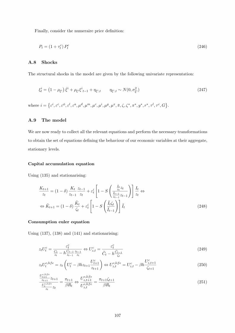
Finally, consider the numeraire price definition:
Pt = (1 + τ ct ) P c
t (246)
A.8 Shocks
The structural shocks in the model are given by the following univariate representation:
ξit =
(1− ρξi
)ξi + ρξiξi
t−1 + ηξi,t ηξi,t ∼ N(0, σ2ξi) (247)
where i ={εi, εc, εφ, εl, εa, µd, µm, µc, µi, µg, µx, π, ζ, ζ∗, π∗, y∗, r∗, τ l, τ c, G
}.
A.9 The model
We are now ready to collect all the relevant equations and perform the necessary transformations
to obtain the set of equations defining the behaviour of our economic variables at their aggregate,
stationary levels.
Capital accumulation equation
Using (135) and stationarising:
Kt+1
zt= (1− δ)
Kt
zt−1
zt−1
zt+ εi
t
[1− S
(Itzt
zt
It−1
zt−1zt−1
)]It
zt⇔
⇔ Kt+1 = (1− δ)Kt
ζt+ εi
t
[1− S
(Itζt
It−1
)]It (248)
Consumption euler equation
Using (137), (138) and (141) and stationarising:
ztUct =
εct
Ctzt− hCt−1
zt−1
zt−1
zt
⇔ U cz,t =
εct
Ct − h Ct−1
ζt
(249)
ztUc,lifet = zt
(U c
t − βhzt+1U c
t+1
zt+1
)⇔ U c,life
z,t = U cz,t − βh
U cz,t+1
ζt+1(250)
Uc,lifet+1
zt+1zt+1
Uc,lifetzt
zt
=πt+1
βRt⇔ U c,life
z,t+1
U c,lifez,t
=πt+1ζt+1
βRt(251)
107

UIP condition
From (143):
Rt = R∗t Φ
(b∗t+1, ε
φt
)(252)
Investment decision
Using (145) and stationarising:
Qtεit
[1− S
(Itzt
zt
It−1
zt−1zt−1
)− S′
(Itzt
zt
It−1
zt−1zt−1
)Itzt
zt
It−1
zt−1zt−1
]+
Qt+1πt+1εit+1
Rt×
× S′( It+1
zt+1zt+1
Itzt
zt
) ( It+1
zt+1zt+1
Itzt
zt
)2
= pit ⇔ Qtε
it
[1− S
(Itζt
It−1
)− S′
(Itζt
It−1
)Itζt
It−1
]+
+Qt+1πt+1ε
it+1
RtS′
(It+1ζt+1
It
)(It+1ζt+1
It
)2
= pit (253)
Capital stock decision
Using (147) and stationarising:
rkt+1 = Qt
Rt
πt+1−Qt+1 (1− δ) (254)
Wage decision
Using (148), (150), (151) and (154) and stationarising:
U lt = −εl
tLσlt (255)
Lt+s =
Wt+s
Pt+szt+s
Wt+s
Pt+szt+s
µwµw−1
Lt+s ⇔ Lt+s =(
wt+s
¨wt+s
) µwµw−1
Lt+s (256)
Wt+s
Pt+szt+s= Xw
t+s
zt+s
zt
W 0t
Pt+szt+s
Pt
Pt= Xw
t+s
W 0t
ztPt
Pt
Pt+s⇔ ¨wt+s =
Xwt+s
πt+s...πt+1
¨w0t (257)
Et
∞∑
s=0
(βξw)s Lt+s
{U l
t+sµw + ¨w0t U
c,lifez,t+s
(1− τ l
t+s
) Xwt+s
πt+s...πt+1
}= 0 (258)
108
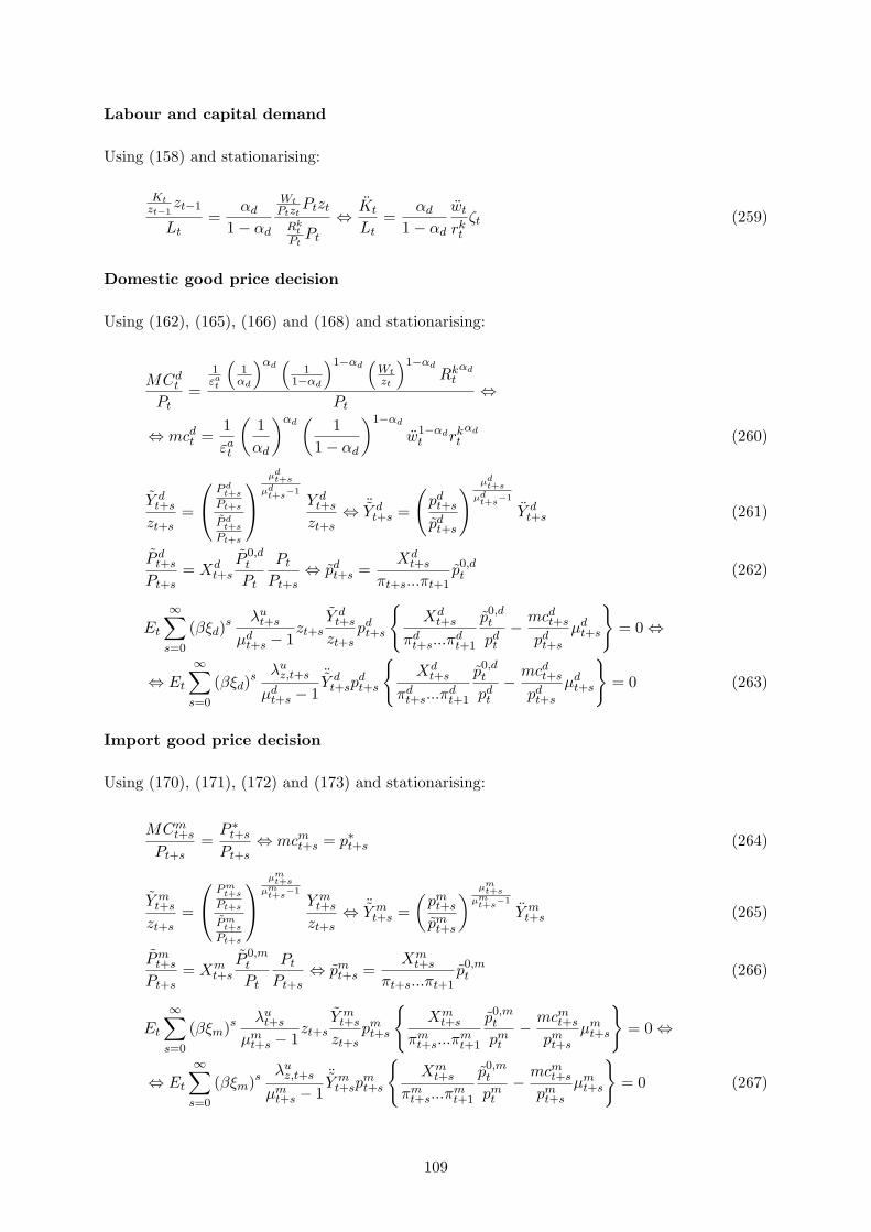
Labour and capital demand
Using (158) and stationarising:
Ktzt−1
zt−1
Lt=
αd
1− αd
WtPtzt
Ptzt
Rkt
PtPt
⇔ Kt
Lt=
αd
1− αd
wt
rkt
ζt (259)
Domestic good price decision
Using (162), (165), (166) and (168) and stationarising:
MCdt
Pt=
1εat
(1
αd
)αd(
11−αd
)1−αd(
Wtzt
)1−αd
Rktαd
Pt⇔
⇔ mcdt =
1εat
(1αd
)αd(
11− αd
)1−αd
w1−αdt rk
tαd (260)
Y dt+s
zt+s=
P dt+s
Pt+s
P dt+s
Pt+s
µdt+s
µdt+s−1
Y dt+s
zt+s⇔ ¨Y d
t+s =
(pd
t+s
pdt+s
) µdt+s
µdt+s−1
Y dt+s (261)
P dt+s
Pt+s= Xd
t+s
P 0,dt
Pt
Pt
Pt+s⇔ pd
t+s =Xd
t+s
πt+s...πt+1p0,d
t (262)
Et
∞∑
s=0
(βξd)s λu
t+s
µdt+s − 1
zt+sY d
t+s
zt+spd
t+s
{Xd
t+s
πdt+s...π
dt+1
p0,dt
pdt
− mcdt+s
pdt+s
µdt+s
}= 0 ⇔
⇔ Et
∞∑
s=0
(βξd)s λu
z,t+s
µdt+s − 1
¨Y dt+sp
dt+s
{Xd
t+s
πdt+s...π
dt+1
p0,dt
pdt
− mcdt+s
pdt+s
µdt+s
}= 0 (263)
Import good price decision
Using (170), (171), (172) and (173) and stationarising:
MCmt+s
Pt+s=
P ∗t+s
Pt+s⇔ mcm
t+s = p∗t+s (264)
Y mt+s
zt+s=
P mt+s
Pt+s
P mt+s
Pt+s
µmt+s
µmt+s−1
Y mt+s
zt+s⇔ ¨Y m
t+s =(
pmt+s
pmt+s
) µmt+s
µmt+s−1
Y mt+s (265)
Pmt+s
Pt+s= Xm
t+s
P 0,mt
Pt
Pt
Pt+s⇔ pm
t+s =Xm
t+s
πt+s...πt+1p0,m
t (266)
Et
∞∑
s=0
(βξm)s λut+s
µmt+s − 1
zt+sY m
t+s
zt+spm
t+s
{Xm
t+s
πmt+s...π
mt+1
p0,mt
pmt
− mcmt+s
pmt+s
µmt+s
}= 0 ⇔
⇔ Et
∞∑
s=0
(βξm)s λuz,t+s
µmt+s − 1
¨Y mt+sp
mt+s
{Xm
t+s
πmt+s...π
mt+1
p0,mt
pmt
− mcmt+s
pmt+s
µmt+s
}= 0 (267)
109
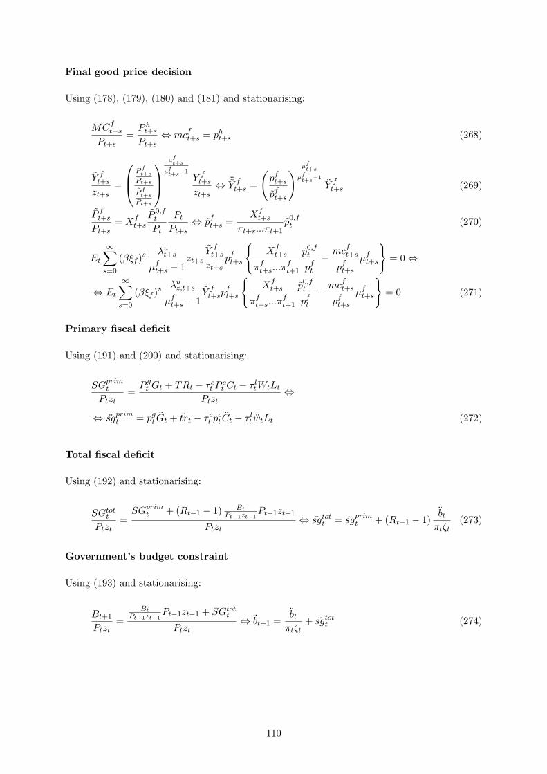
Final good price decision
Using (178), (179), (180) and (181) and stationarising:
MCft+s
Pt+s=
P ht+s
Pt+s⇔ mcf
t+s = pht+s (268)
Y ft+s
zt+s=
P ft+s
Pt+s
P ft+s
Pt+s
µft+s
µft+s−1
Y ft+s
zt+s⇔ ¨Y f
t+s =
(pf
t+s
pft+s
) µft+s
µft+s−1
Y ft+s (269)
P ft+s
Pt+s= Xf
t+s
P 0,ft
Pt
Pt
Pt+s⇔ pf
t+s =Xf
t+s
πt+s...πt+1p0,f
t (270)
Et
∞∑
s=0
(βξf )s λut+s
µft+s − 1
zt+sY f
t+s
zt+spf
t+s
{Xf
t+s
πft+s...π
ft+1
p0,ft
pft
− mcft+s
pft+s
µft+s
}= 0 ⇔
⇔ Et
∞∑
s=0
(βξf )s λuz,t+s
µft+s − 1
¨Y ft+sp
ft+s
{Xf
t+s
πft+s...π
ft+1
p0,ft
pft
− mcft+s
pft+s
µft+s
}= 0 (271)
Primary fiscal deficit
Using (191) and (200) and stationarising:
SGprimt
Ptzt=
P gt Gt + TRt − τ c
t P ct Ct − τ l
tWtLt
Ptzt⇔
⇔ sgprimt = pg
t Gt + trt − τ ct pc
tCt − τ lt wtLt (272)
Total fiscal deficit
Using (192) and stationarising:
SGtott
Ptzt=
SGprimt + (Rt−1 − 1) Bt
Pt−1zt−1Pt−1zt−1
Ptzt⇔ sgtot
t = sgprimt + (Rt−1 − 1)
bt
πtζt(273)
Government’s budget constraint
Using (193) and stationarising:
Bt+1
Ptzt=
BtPt−1zt−1
Pt−1zt−1 + SGtott
Ptzt⇔ bt+1 =
bt
πtζt+ sgtot
t (274)
110
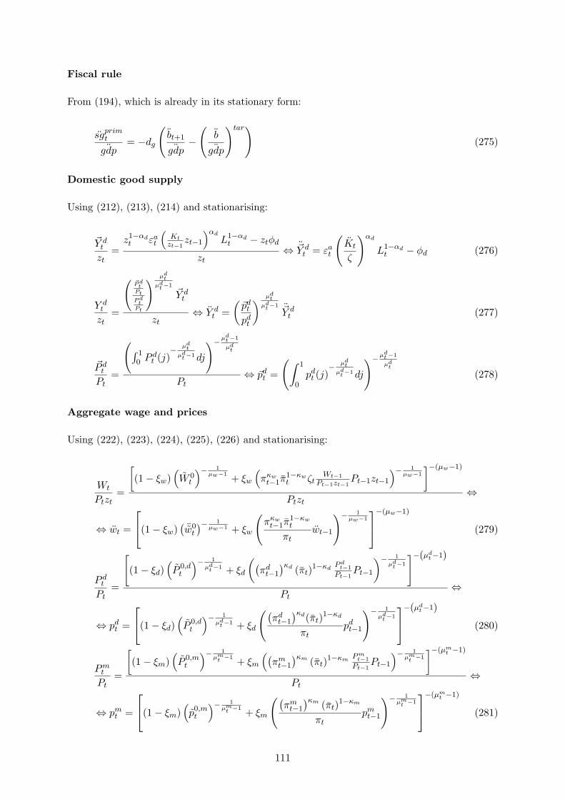
Fiscal rule
From (194), which is already in its stationary form:
sgprimt
¨gdp= −dg
(bt+1
¨gdp−
(b¨gdp
)tar)(275)
Domestic good supply
Using (212), (213), (214) and stationarising:
~Y dt
zt=
z1−αdt εa
t
(Kt
zt−1zt−1
)αd
L1−αdt − ztφd
zt⇔ ~Y d
t = εat
(Kt
ζ
)αd
L1−αdt − φd (276)
Y dt
zt=
(~Pdt
Pt
Pdt
Pt
) µdt
µdt−1
~Y dt
zt⇔ Y d
t =(
~pdt
pdt
) µdt
µdt−1
~Y dt (277)
~P dt
Pt=
(∫ 10 P d
t (j)− µd
tµd
t−1 dj
)−µdt−1
µdt
Pt⇔ ~pd
t =
(∫ 1
0pd
t (j)− µd
tµd
t−1 dj
)−µdt−1
µdt
(278)
Aggregate wage and prices
Using (222), (223), (224), (225), (226) and stationarising:
Wt
Ptzt=
[(1− ξw)
(W 0
t
)− 1µw−1 + ξw
(πκw
t−1π1−κwt ζt
Wt−1
Pt−1zt−1Pt−1zt−1
)− 1µw−1
]−(µw−1)
Ptzt⇔
⇔ wt =
(1− ξw)
( ¨w0t
)− 1µw−1 + ξw
(πκw
t−1π1−κwt
πtwt−1
)− 1µw−1
−(µw−1)
(279)
P dt
Pt=
[(1− ξd)
(P 0,d
t
)− 1
µdt−1 + ξd
((πd
t−1
)κd (πt)1−κd
P dt−1
Pt−1Pt−1
)− 1
µdt−1
]−(µdt−1)
Pt⇔
⇔ pdt =
(1− ξd)
(P 0,d
t
)− 1
µdt−1 + ξd
((πd
t−1
)κd(πt)1−κd
πtpd
t−1
)− 1
µdt−1
−(µd
t−1)
(280)
Pmt
Pt=
[(1− ξm)
(P 0,m
t
)− 1µm
t −1 + ξm
((πm
t−1
)κm (πt)1−κm P m
t−1
Pt−1Pt−1
)− 1µm
t −1
]−(µmt −1)
Pt⇔
⇔ pmt =
(1− ξm)
(p0,m
t
)− 1µm
t −1 + ξm
((πm
t−1
)κm (πt)1−κm
πtpm
t−1
)− 1µm
t −1
−(µm
t −1)
(281)
111
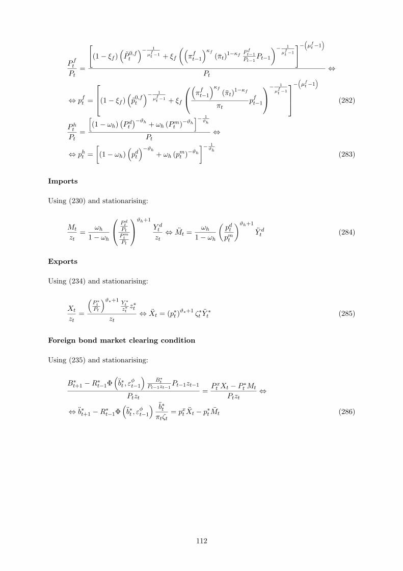
P ft
Pt=
[(1− ξf )
(P 0,f
t
)− 1
µft −1 + ξf
((πf
t−1
)κf
(πt)1−κf
P ft−1
Pt−1Pt−1
)− 1
µft −1
]−(µf
t−1)
Pt⇔
⇔ pft =
(1− ξf )
(p0,f
t
)− 1
µft −1 + ξf
(πf
t−1
)κf
(πt)1−κf
πtpf
t−1
− 1
µft −1
−(µf
t−1)
(282)
P ht
Pt=
[(1− ωh)
(P d
t
)−ϑh + ωh (Pmt )−ϑh
]− 1ϑh
Pt⇔
⇔ pht =
[(1− ωh)
(pd
t
)−ϑh
+ ωh (pmt )−ϑh
]− 1ϑh
(283)
Imports
Using (230) and stationarising:
Mt
zt=
ωh
1− ωh
P dt
Pt
P mt
Pt
ϑh+1
Y dt
zt⇔ Mt =
ωh
1− ωh
(pd
t
pmt
)ϑh+1
Y dt (284)
Exports
Using (234) and stationarising:
Xt
zt=
(P ∗tPt
)ϑ∗+1 Y ∗tz∗t
z∗tzt
⇔ Xt = (p∗t )ϑ∗+1 ζ∗t Y ∗
t (285)
Foreign bond market clearing condition
Using (235) and stationarising:
B∗t+1 −R∗
t−1Φ(b∗t , ε
φt−1
)B∗t
Pt−1zt−1Pt−1zt−1
Ptzt=
P xt Xt − P ∗
t Mt
Ptzt⇔
⇔ b∗t+1 −R∗t−1Φ
(b∗t , ε
φt−1
) b∗tπtζt
= pxt Xt − p∗t Mt (286)
112

Aggregate resource constraint
Using (238) and stationarising:
Y dt
zt= (1− ωh)
P ht
Pt
P dt
Pt
ϑh+1 (Ct + It + Gt + Xt
zt
)⇔
⇔ Y dt = (1− ωh)
(ph
t
pdt
)ϑh+1 (Ct + It + Gt + Xt
)(287)
GDP definition
Using (239) and stationarising:
GDPt
Ptzt=
PtCt + P gt Gt + P i
t It + P xt Xt − Pm
t Mt
Ptzt⇔
⇔ ¨gdpt = Ct + pgt Gt + pi
tIt + pxt Xt − pm
t Mt (288)
Inflation identities
Using (240) and stationarising:
πwt
πt=
wtzt
ztwt−1
zt−1zt−1
=wt
wt−1ζt (289)
From (241), (242), (243), (244), (245), which are already stationary:
πdt
πt=
pdt
pdt−1
(290)
πmt
πt=
pmt
pmt−1
(291)
πft
πt=
pft
pft−1
(292)
πht
πt=
pht
pht−1
(293)
π∗tπt
=p∗t
p∗t−1
(294)
113

Numeraire definition
Using (246) and stationarising:
Pt
Pt=
(1 + τ ct ) P c
t
Pt⇔ 1 = (1 + τ c
t ) pct (295)
Shocks
Using (247), which is assumed to be already stationary:
ξt = (1− ρξ) ξ + ρξξt−1 + ηξ,t (296)
A.10 The steady-state model
We now derive the steady-state version of the model. The numeraire inflation rate is considered
to be at its target level, π = π. Furthermore, it is assumed that p∗ = 1 and that ζ∗ = 1.
Capital accumulation equation
Equation (248) in the steady-state is given by:
K = (1− δ)K
ζ+ εi
[1− S
(I
Iζ
)]I = (1− δ)
K
ζ+ [1− S (ζ)] I =
= (1− δ)K
ζ+ I ⇔ I =
(1− 1− δ
ζ
)K (297)
where we have used (360).
Consumption euler equation
Equations (249), (250) and (251) in the steady-state are given by:
U cz =
εc
C − h Cζ
=1
C(1− h1
ζ
) (298)
U c,lifez = U c
z − βhU c
z
ζ=
1
C(1− h1
ζ
) − βh
1
C(1−h 1
ζ
)
ζ=
ζ (ζ − βh)C (ζ − h)
(299)
U cz
U czζ
=π
βR⇔ R =
πζ
β(300)
where we have used (360).
114

UIP condition
Equation (252) in the steady-state is given by:
R = R∗Φ(b∗, εφ
)(301)
Assuming that R = R∗ we must have Φ(b∗, εφ
)= 1, which can only happen if εφ = 0 and:
b∗ = 0 (302)
Investment decision
Equation (253) in the steady-state is given by:
Qεi
[1− S
(Iζ
I
)− S′
(Iζ
I
)Iζ
I
]+ Q
π
RεiS′
(Iζ
I
)(Iζ
I
)2
= pi ⇔
⇔ Q[1− S (ζ)− S′ (ζ) ζ
]+ Q
π
RS′ (ζ) ζ2 = pi ⇔ Q = pi (303)
where we have used (360).
Capital stock decision
Equation (254) in the steady-state is given by:
rk = QR
π−Q (1− δ) ⇔ rk = pi
(R
π− (1− δ)
)(304)
where we have used (303).
Wage decision
Equations (255), (256), (257) and (258) in the steady-state are given by:
U l = −Lσl (305)
L =(
w¨w
) µwµw−1
L =( ¨w0
¨w
) µwµw−1
L = L (306)
¨w =Xw
πs−1¨w0 = ¨w0 (307)
115
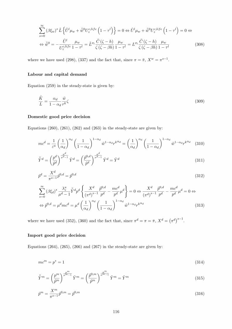
∞∑
s=0
(βξw)s L{
U lµw + ¨w0U c,lifez
(1− τ l
)}= 0 ⇔ U lµw + ¨w0U c,life
z
(1− τ l
)= 0 ⇔
⇔ ¨w0 = − U l
U c,lifez
µw
1− τ l= Lσl
C (ζ − h)ζ (ζ − βh)
µw
1− τ l= Lσl
C (ζ − h)ζ (ζ − βh)
µw
1− τ l(308)
where we have used (298), (337) and the fact that, since π = π, Xw = πs−1.
Labour and capital demand
Equation (259) in the steady-state is given by:
K
L=
αd
1− αd
w
rkζ (309)
Domestic good price decision
Equations (260), (261), (262) and (263) in the steady-state are given by:
mcd =1εa
(1αd
)αd(
11− αd
)1−αd
w1−αdrkαd =(
1αd
)αd(
11− αd
)1−αd
w1−αdrkαd (310)
¨Y d =(
pd
pd
) µd
µd−1
Y d =(
p0,d
pd
) µd
µd−1
Y d = Y d (311)
pd =Xd
πs−1p0,d = p0,d (312)
∞∑
s=0
(βξd)s λu
z
µd − 1¨Y dpd
{Xd
(πd)s−1
p0,d
pd− mcd
pdµd
}= 0 ⇔ Xd
(πd)s−1
p0,d
pd− mcd
pdµd = 0 ⇔
⇔ p0,d = µdmcd = µd
(1αd
)αd(
11− αd
)1−αd
w1−αdrkαd (313)
where we have used (352), (360) and the fact that, since πd = π = π, Xd =(πd
)s−1.
Import good price decision
Equations (264), (265), (266) and (267) in the steady-state are given by:
mcm = p∗ = 1 (314)
¨Y m =(
pm
pm
) µm
µm−1
Y m =(
p0,m
pm
) µm
µm−1
Y m = Y m (315)
pm =Xm
πs−1p0,m = p0,m (316)
116

∞∑
s=0
(βξm)s λuz
µm − 1¨Y mpm
{Xm
(πm)s−1
p0,m
pm− mcm
pmµm
}= 0 ⇔ Xm
(πm)s−1
p0,m
pm−
− mcm
pmµm = 0 ⇔ p0,m = µmmcm = µm (317)
where we have used (353) and the fact that, since πm = π = π, Xm = (πm)s−1.
Final good price decision
Equations (268), (269), (270) and (271) in the steady-state are given by:
mcf = ph (318)
¨Y f =(
pf
pf
) µf
µf−1
Y f =(
p0,f
pf
) µf
µf−1
Y f = Y f (319)
pf =Xf
πs−1p0,f = p0,f (320)
∞∑
s=0
(βξf )s λuz
µf − 1¨Y fpf
{Xf
(πf )s−1
p0,f
pf− mcf
pfµf
}= 0 ⇔ Xf
(πf )s−1
p0,f
pf−
− mcf
pfµf = 0 ⇔ p0,f = µfmcf = µf (321)
where we have used (354) and the fact that, since πf = π = π, Xf =(πf
)s−1.
Primary fiscal deficit
Equation (272) in the steady-state is given by:
sgprim = pgG + tr − τ cpcC − τ lwL (322)
Total fiscal deficit
Equation (273) in the steady-state is given by:
sgtot = sgprim + (R− 1)b
πζ(323)
117
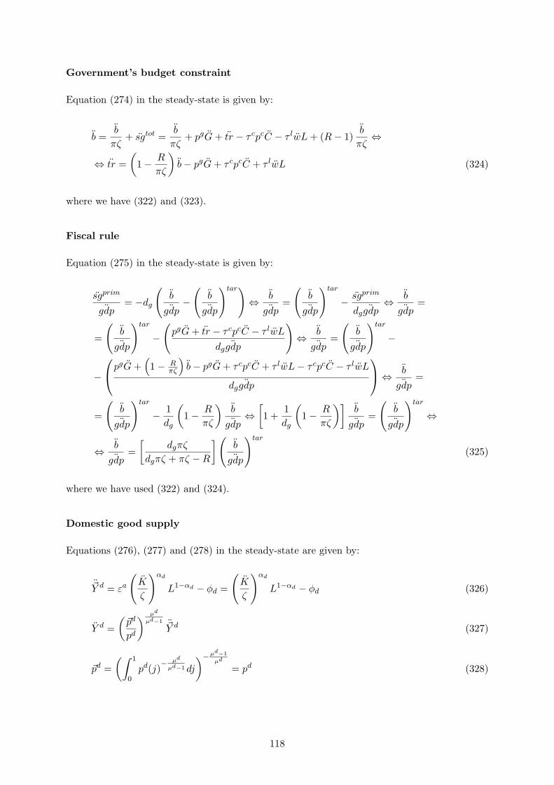
Government’s budget constraint
Equation (274) in the steady-state is given by:
b =b
πζ+ sgtot =
b
πζ+ pgG + tr − τ cpcC − τ lwL + (R− 1)
b
πζ⇔
⇔ tr =(
1− R
πζ
)b− pgG + τ cpcC + τ lwL (324)
where we have (322) and (323).
Fiscal rule
Equation (275) in the steady-state is given by:
sgprim
¨gdp= −dg
(b¨gdp−
(b¨gdp
)tar)⇔ b
¨gdp=
(b¨gdp
)tar
− sgprim
dg¨gdp
⇔ b¨gdp
=
=
(b¨gdp
)tar
−(
pgG + tr − τ cpcC − τ lwL
dg¨gdp
)⇔ b
¨gdp=
(b¨gdp
)tar
−
−pgG +
(1− R
πζ
)b− pgG + τ cpcC + τ lwL− τ cpcC − τ lwL
dg¨gdp
⇔ b
¨gdp=
=
(b¨gdp
)tar
− 1dg
(1− R
πζ
)b¨gdp
⇔[1 +
1dg
(1− R
πζ
)]b¨gdp
=
(b¨gdp
)tar
⇔
⇔ b¨gdp
=[
dgπζ
dgπζ + πζ −R
] (b¨gdp
)tar
(325)
where we have used (322) and (324).
Domestic good supply
Equations (276), (277) and (278) in the steady-state are given by:
~Y d = εa
(K
ζ
)αd
L1−αd − φd =
(K
ζ
)αd
L1−αd − φd (326)
Y d =(
~pd
pd
) µd
µd−1~Y d (327)
~pd =(∫ 1
0pd(j)
− µd
µd−1 dj
)−µd−1
µd
= pd (328)
118
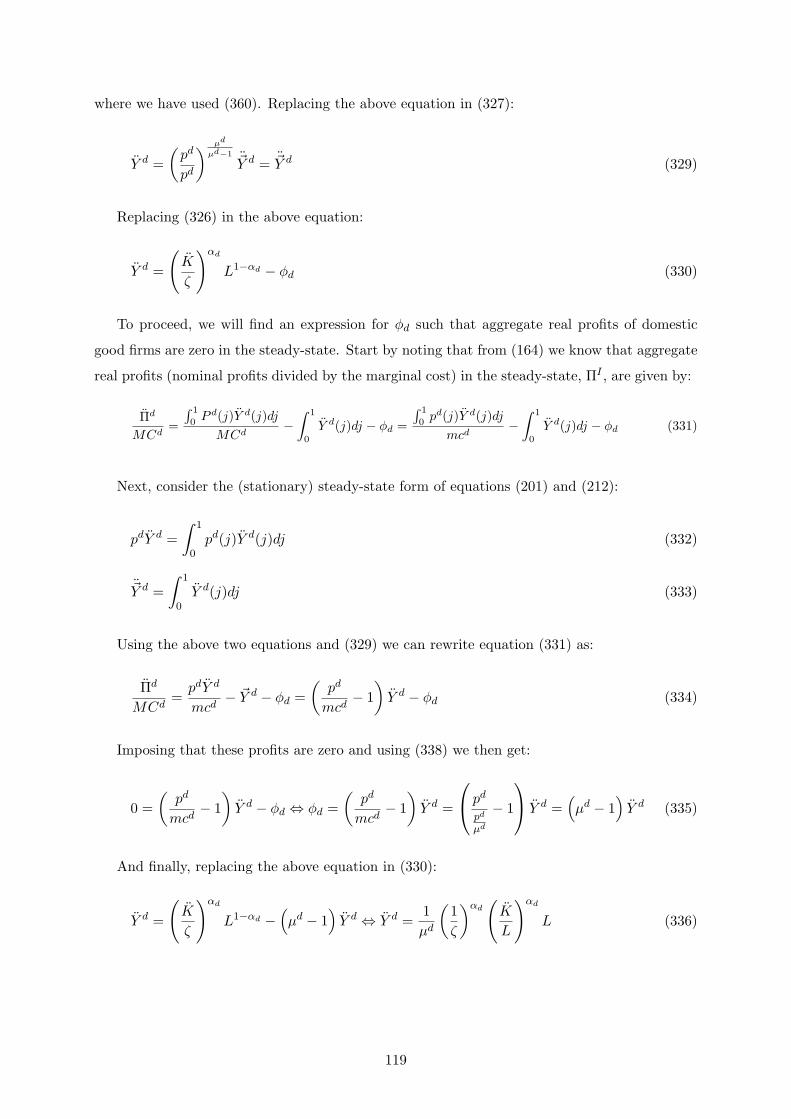
where we have used (360). Replacing the above equation in (327):
Y d =(
pd
pd
) µd
µd−1~Y d = ~Y d (329)
Replacing (326) in the above equation:
Y d =
(K
ζ
)αd
L1−αd − φd (330)
To proceed, we will find an expression for φd such that aggregate real profits of domestic
good firms are zero in the steady-state. Start by noting that from (164) we know that aggregate
real profits (nominal profits divided by the marginal cost) in the steady-state, ΠI , are given by:
Πd
MCd=
∫ 1
0P d(j)Y d(j)dj
MCd−
∫ 1
0
Y d(j)dj − φd =
∫ 1
0pd(j)Y d(j)dj
mcd−
∫ 1
0
Y d(j)dj − φd (331)
Next, consider the (stationary) steady-state form of equations (201) and (212):
pdY d =∫ 1
0pd(j)Y d(j)dj (332)
~Y d =∫ 1
0Y d(j)dj (333)
Using the above two equations and (329) we can rewrite equation (331) as:
Πd
MCd=
pdY d
mcd− ~Y d − φd =
(pd
mcd− 1
)Y d − φd (334)
Imposing that these profits are zero and using (338) we then get:
0 =(
pd
mcd− 1
)Y d − φd ⇔ φd =
(pd
mcd− 1
)Y d =
pd
pd
µd
− 1
Y d =
(µd − 1
)Y d (335)
And finally, replacing the above equation in (330):
Y d =
(K
ζ
)αd
L1−αd −(µd − 1
)Y d ⇔ Y d =
1µd
(1ζ
)αd(
K
L
)αd
L (336)
119

Aggregate wage and prices
Equations (279), (280), (281), (282) and (283) in the steady-state are given by:
w =
[(1− ξw)
( ¨w0)− 1
µw−1 + ξw
(πκw π1−κw
πw
)− 1µw−1
]−(µw−1)
⇔ (w)−1
(µw−1) =
= (1− ξw)( ¨w0
)− 1µw−1 + ξw (w)−
1µw−1 ⇔ (1− ξw) w
− 1(µw−1) = (1− ξw)
( ¨w0)− 1
µw−1 ⇔
⇔ w = ¨w0 = LσlC (ζ − h)ζ (ζ − βh)
µw
1− τ l⇔ L =
(w
(1− τ l
)
µw
ζ − βh
ζ − hζ
) 1σl
(1C
) 1σl
(337)
pd =
(1− ξd)
(p0,d
)− 1µd−1 + ξd
((πd
)κd π1−κd
πpd
)− 1µd−1
−(µd−1)
⇔ (pd
)− 1µd−1 =
= (1− ξd)(p0,d
)− 1µd−1 + ξd
(pd
)− 1µd−1 ⇔ (1− ξd)
(pd
)− 1µd−1 = (1− ξd)
(p0,d
)− 1µd−1 ⇔ pd =
= p0,d = µd
(1αd
)αd(
11− αd
)1−αd
w1−αdrkαd ⇔ w =(
pd
µdrkαdααd
d (1− αd)1−αd
) 11−αd
(338)
pm =
[(1− ξm)
(p0,m
)− 1µm−1 + ξm
((πm)κm π1−κm
πpm
)− 1µm−1
]−(µm−1)
⇔ (pm)−1
µm−1 =
= (1− ξm)(p0,m
)− 1µm−1 + ξm (pm)−
1µm−1 ⇔ pm = p0,m = µm (339)
pf =
(1− ξf )
(p0,f
)− 1
µf−1 + ξf
((πf
)κf π1−κf
πpf
)− 1
µf−1
−(µf−1)
⇔(pf
)− 1
µf−1 =
= (1− ξf )(p0,f
)− 1
µf−1 + ξf
(pf
)− 1
µf−1 ⇔ pf = p0,f = µfph (340)
ph =[(1− ωh)
(pd
)−ϑh
+ ωh (pm)−ϑh
]− 1ϑh ⇔
(ph
)−ϑh
=
= (1− ωh)(pd
)−ϑh
+ ωh (pm)−ϑh ⇔ pd =
[(ph
)−ϑh − ωh (pm)−ϑh
1− ωh
]− 1ϑh
(341)
where we have used (308), (313), (352), (317), (353), (321) and (354). Using (340) we can write:
pc = µcph ⇔ ph =pc
µc(342)
pi = µiph (343)
pg = µgph (344)
px = µxph (345)
120
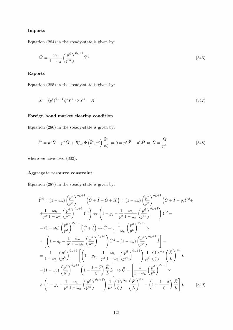
Imports
Equation (284) in the steady-state is given by:
M =ωh
1− ωh
(pd
pm
)ϑh+1
Y d (346)
Exports
Equation (285) in the steady-state is given by:
X = (p∗)ϑ∗+1 ζ∗Y ∗ ⇔ Y ∗ = X (347)
Foreign bond market clearing condition
Equation (286) in the steady-state is given by:
b∗ = pxX − p∗M + R∗t−1Φ
(b∗, εφ
) b∗
πζ⇔ 0 = pxX − p∗M ⇔ X =
M
px(348)
where we have used (302).
Aggregate resource constraint
Equation (287) in the steady-state is given by:
Y d = (1− ωh)(
ph
pd
)ϑh+1 (C + I + G + X
)= (1− ωh)
(ph
pd
)ϑh+1 (C + I + gyY
d+
+1px
ωh
1− ωh
(pd
pm
)ϑh+1
Y d
)⇔
(1− gy − 1
px
ωh
1− ωh
(pd
pm
)ϑh+1)
Y d =
= (1− ωh)(
ph
pd
)ϑh+1 (C + I
)⇔ C =
11− ωh
(pd
ph
)ϑh+1
×
×[(
1− gy − 1px
ωh
1− ωh
(pd
pm
)ϑh+1)
Y d − (1− ωh)(
ph
pd
)ϑh+1
I
]=
=1
1− ωh
(pd
ph
)ϑh+1[(
1− gy − 1px
ωh
1− ωh
(pd
pm
)ϑh+1)
1µd
(1ζ
)αd(
K
L
)αd
L−
− (1− ωh)(
ph
pd
)ϑh+1 (1− 1− δ
ζ
)K
LL
]⇔ C =
[1
1− ωh
(pd
ph
)ϑh+1
×
×(
1− gy − 1px
ωh
1− ωh
(pd
pm
)ϑh+1)
1µd
(1ζ
)αd(
K
L
)αd
−(
1− 1− δ
ζ
)K
L
]L (349)
121
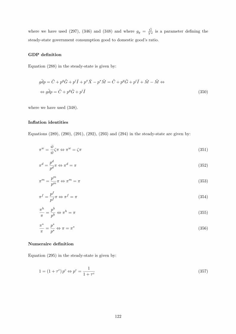
where we have used (297), (346) and (348) and where gy = GY d
is a parameter defining the
steady-state government consumption good to domestic good’s ratio.
GDP definition
Equation (288) in the steady-state is given by:
¨gdp = C + pgG + piI + pxX − p∗M = C + pgG + piI + M − M ⇔
⇔ ¨gdp = C + pgG + piI (350)
where we have used (348).
Inflation identities
Equations (289), (290), (291), (292), (293) and (294) in the steady-state are given by:
πw =w
wζπ ⇔ πw = ζπ (351)
πd =pd
pdπ ⇔ πd = π (352)
πm =pm
pmπ ⇔ πm = π (353)
πf =pf
pfπ ⇔ πf = π (354)
πh
π=
ph
ph⇔ πh = π (355)
π∗
π=
p∗
p∗⇔ π = π∗ (356)
Numeraire definition
Equation (295) in the steady-state is given by:
1 = (1 + τ c) pc ⇔ pc =1
1 + τ c(357)
122
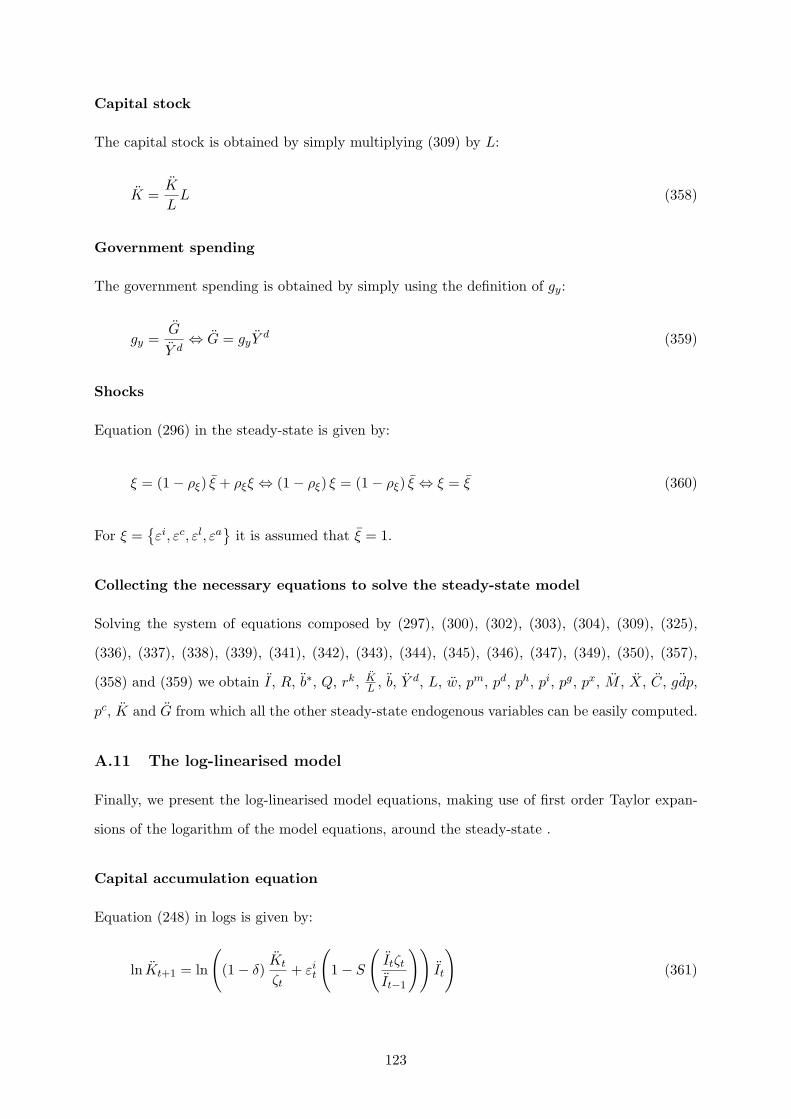
Capital stock
The capital stock is obtained by simply multiplying (309) by L:
K =K
LL (358)
Government spending
The government spending is obtained by simply using the definition of gy:
gy =G
Y d⇔ G = gyY
d (359)
Shocks
Equation (296) in the steady-state is given by:
ξ = (1− ρξ) ξ + ρξξ ⇔ (1− ρξ) ξ = (1− ρξ) ξ ⇔ ξ = ξ (360)
For ξ ={εi, εc, εl, εa
}it is assumed that ξ = 1.
Collecting the necessary equations to solve the steady-state model
Solving the system of equations composed by (297), (300), (302), (303), (304), (309), (325),
(336), (337), (338), (339), (341), (342), (343), (344), (345), (346), (347), (349), (350), (357),
(358) and (359) we obtain I, R, b∗, Q, rk, KL , b, Y d, L, w, pm, pd, ph, pi, pg, px, M , X, C, ¨gdp,
pc, K and G from which all the other steady-state endogenous variables can be easily computed.
A.11 The log-linearised model
Finally, we present the log-linearised model equations, making use of first order Taylor expan-
sions of the logarithm of the model equations, around the steady-state .
Capital accumulation equation
Equation (248) in logs is given by:
ln Kt+1 = ln
((1− δ)
Kt
ζt+ εi
t
(1− S
(Itζt
It−1
))It
)(361)
123

Applying the Taylor approximation to the previous equation:
ln Kt+1 ' ln K + ˆKt+1 (362)
ln
((1− δ)
Kt
ζt+ εi
t
(1− S
(Itζt
It−1
))It
)' ln K +
(1− δ) 1ζ
(1− δ) Kζ + I
Kt − K
KK−
−(1−δ)K
ζ2
(1− δ) Kζ + I
ζt − ζ
ζζ +
I
(1− δ) Kζ + I
εit − εi
εi+
1
(1− δ) Kζ + I
It − I
II =
= ln K +(1− δ) K
ζ
(1− δ) Kζ + I
(ˆKt − ζt
)+
I
(1− δ) Kζ + I
(εit + ˆIt
)=
= ln K +1− δ
ζ
(ˆKt − ζt
)+
(1− 1− δ
ζ
)(εit + ˆIt
)(363)
where we have used (297) and (360). Replacing (362)-(363) in (361):
ˆKt+1 =1− δ
ζ
(ˆKt − ζt
)+
(1− 1− δ
ζ
) (εit + ˆIt
)(364)
Consumption euler equation
Equation (249) in logs is given by:
ln U cz,t = ln εc
t − ln
(Ct − h
Ct−1
ζt
)(365)
Applying the Taylor approximation to the previous equation:
ln U cz,t ' ln U c
z + U cz,t (366)
ln εct ' ln εc + εc
t (367)
ln
(Ct − h
Ct−1
ζt
)' ln
(C − h
C
ζ
)+
1
C − h Cζ
(C ˆCt − hC
ζˆCt−1 + h
C
ζ2ζζt
)=
= ln
(C − h
C
ζ
)+
11− h
ζ
(ˆCt − h
ζˆCt−1 +
h
ζζt
)= ln
(C − h
C
ζ
)+
+1
ζ − h
(ζ ˆCt − h ˆCt−1 + hζt
)= ln
(C − h
C
ζ
)+
ζ
ζ − hˆCt − h
ζ − hˆCt−1 +
h
ζ − hζt (368)
124

Replacing (366)-(368) in (365):
U cz,t = εc
t −ζ
ζ − hˆCt +
h
ζ − hˆCt−1 − h
ζ − hζt (369)
Equation (250) in logs is given by:
ln U c,lifez,t = ln
(U c
z,t − βhU c
z,t+1
ζt+1
)(370)
Applying the Taylor approximation to the previous equation:
ln U c,lifez,t ' lnU c,life
z + U c,lifez,t (371)
ln(
U cz,t − βh
U cz,t+1
ζt+1
)' ln
(U c
z − βhU c
z
ζ
)+
1
U cz − βhUc
zζ
(U c
z U c,iz,t −
βh
ζU c
z U c,iz,t+1+
+βhU c
z
ζ2ζζt+1
)= ln
(U c
z − βhU c
z
ζ
)+
ζ
ζ − βhU c,i
z,t −βh
ζ − βhU c,i
z,t+1 +βh
ζ − βhζt+1 (372)
Replacing (371)-(372) in (370):
U c,lifez,t =
ζ
ζ − βhU c,i
z,t −βh
ζ − βhU c,i
z,t+1 +βh
ζ − βhζt+1 (373)
Replacing (369) in (373):
U c,lifez,t =
ζ
ζ − βh
(εct −
ζ
ζ − hˆCt +
h
ζ − hˆCt−1 − h
ζ − hζt
)− βh
ζ − βh
(εct+1 −
ζ
ζ − hˆCt+1+
+h
ζ − hˆCt − h
ζ − hζt+1
)+
βh
ζ − βhζt+1 =
ζ
ζ − βhεct −
ζ2
(ζ − βh) (ζ − h)ˆCt+
+ζh
(ζ − βh) (ζ − h)ˆCt−1 − ζh
(ζ − βh) (ζ − h)ζt − βh
ζ − βhεct+1 +
βhζ
(ζ − βh) (ζ − h)ˆCt+1−
− βh2
(ζ − βh) (ζ − h)ˆCt +
βh2
(ζ − βh) (ζ − h)ζt+1 +
βh
ζ − βhζt+1 =
ζ
ζ − βhεct−
−(ζ2 + βh2
)
(ζ − βh) (ζ − h)ˆCt +
ζh
(ζ − βh) (ζ − h)ˆCt−1 − ζh
(ζ − βh) (ζ − h)ζt − βh
ζ − βhεct+1+
+βhζ
(ζ − βh) (ζ − h)ˆCt+1 +
βhζ
(ζ − βh) (ζ − h)ζt+1 ⇔ ˆCt =
1ζ2 + βh2
[ζh ˆCt−1 − ζhζt−
−βh (ζ − h) εct+1 + βhζ ˆCt+1 + βhζζt+1 + ζ (ζ − h) εc
t − (ζ − βh) (ζ − h) U c,lifez,t
](374)
125
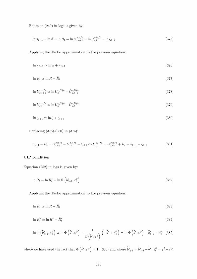
Equation (249) in logs is given by:
ln πt+1 + lnβ − lnRt = ln U c,lifez,t+1 − ln U c,life
z,t − ln ζt+1 (375)
Applying the Taylor approximation to the previous equation:
ln πt+1 ' lnπ + πt+1 (376)
ln Rt ' ln R + Rt (377)
ln U c,lifez,t+1 ' lnU c,life
z + U c,lifez,t+1 (378)
ln U c,lifez,t ' lnU c,life
z + U c,lifez,t (379)
ln ζt+1 ' ln ζ + ζt+1 (380)
Replacing (376)-(380) in (375):
πt+1 − Rt = U c,lifez,t+1 − U c,life
z,t − ζt+1 ⇔ U c,lifez,t = U c,life
z,t+1 + Rt − πt+1 − ζt+1 (381)
UIP condition
Equation (252) in logs is given by:
ln Rt = lnR∗t + lnΦ
(b∗t+1, ε
φt
)(382)
Applying the Taylor approximation to the previous equation:
ln Rt ' ln R + Rt (383)
ln R∗t ' ln R∗ + R∗
t (384)
lnΦ(b∗t+1, ε
φt
)' ln Φ
(b∗, εφ
)+
1
Φ(b∗, εφ
)(−ˆ
b∗ + εφt
)= ln Φ
(b∗, εφ
)− ˆ
b∗t+1 + εφt (385)
where we have used the fact that Φ(b∗, εφ
)= 1, (360) and where ˆ
b∗t+1 = b∗t+1− b∗, εφt = εφ
t − εφ.
126

Replacing (383)-(385) in (382):
Rt = R∗t − ˆ
b∗t+1 + εφt (386)
Investment decision
Equation (253) in logs is given by:
ln
[Qtε
it
[1− S
(Itζt
It−1
)− S′
(Itζt
It−1
)Itζt
It−1
]+
πt+1Qt+1εit+1
RtS′
(It+1ζt+1
It
)×
×(
It+1ζt+1
It
)2 = ln pi
t (387)
Applying the Taylor approximation to each term of the previous equation:
ln
Qtε
it
[1− S
(Itζt
It−1
)− S′
(Itζt
It−1
)Itζt
It−1
]+
Qt+1πt+1εit+1
RtS′
(It+1ζt+1
It
)(It+1ζt+1
It
)2 '
' ln pi +1pi
(εi
(1− S (ζ)− S′ (ζ) ζ
)QQt + Q
(1− S (ζ)− S′ (ζ) ζ
)εiεi
t −Qεi
(S′ (ζ)
1II ˆIt+
+S′ (ζ) I
(−1I2
)I ˆIt−1 + S′ (ζ) ζζt + S′′ (ζ)
ζ
IζI ˆIt + S′′ (ζ) Iζζ
(−1I2
)I ˆIt−1 + S′′ (ζ) ζ2ζt+
+ S′ (ζ)ζ
II ˆIt + S′ (ζ) Iζ
(−1I2
)I ˆIt−1 + S′ (ζ) ζζt
)+
π
RεiS′ (ζ) ζ2QQt+1+
+Qεi
RS′ (ζ) ζ2ππt+1 + Q
π
RS′ (ζ) ζ2εiεi
t+1 + QπεiS′ (ζ) ζ2
(− 1
R2
)RRt + Q
π
Rεiζ2S′′ (ζ)×
×(
ζ
II ˆIt+1 + Iζ
(− 1
I2
)I ˆIt + ζζt+1
)+ Q
π
RεiS′ (ζ) 2ζ
(ζ
II ˆIt+1 + Iζ
(− 1
I2
)I ˆIt + ζζt+1
))=
= ln pi + Qt + εit −
(S′′ (ζ) ζ2 ˆIt − S′′ (ζ) ζ2 ˆIt−1 + S′′ (ζ) ζ2ζt
)+
π
Rζ3S′′ (ζ)
(ˆIt+1 − ˆIt + ζt+1
)=
= ln pi + Qt + εit − S′′ (ζ) ζ2
((1 + β) ˆIt − ˆIt−1 + ζt − β ˆIt+1 − βζt+1
)(388)
ln pit ' ln pi + pi
t (389)
where we have used (360). Replacing (388)-(389) in (387):
Qt + εit − S′′ (ζ) ζ2
((1 + β) ˆIt − ˆIt−1 + ζt − β ˆIt+1 − βζt+1
)= pi
t ⇔
⇔ ˆIt =1
1 + β
[1
S′′ (ζ) ζ2
(Qt + εi
t − pit
)+ ˆIt−1 − ζt + β ˆIt+1 + βζt+1
](390)
127
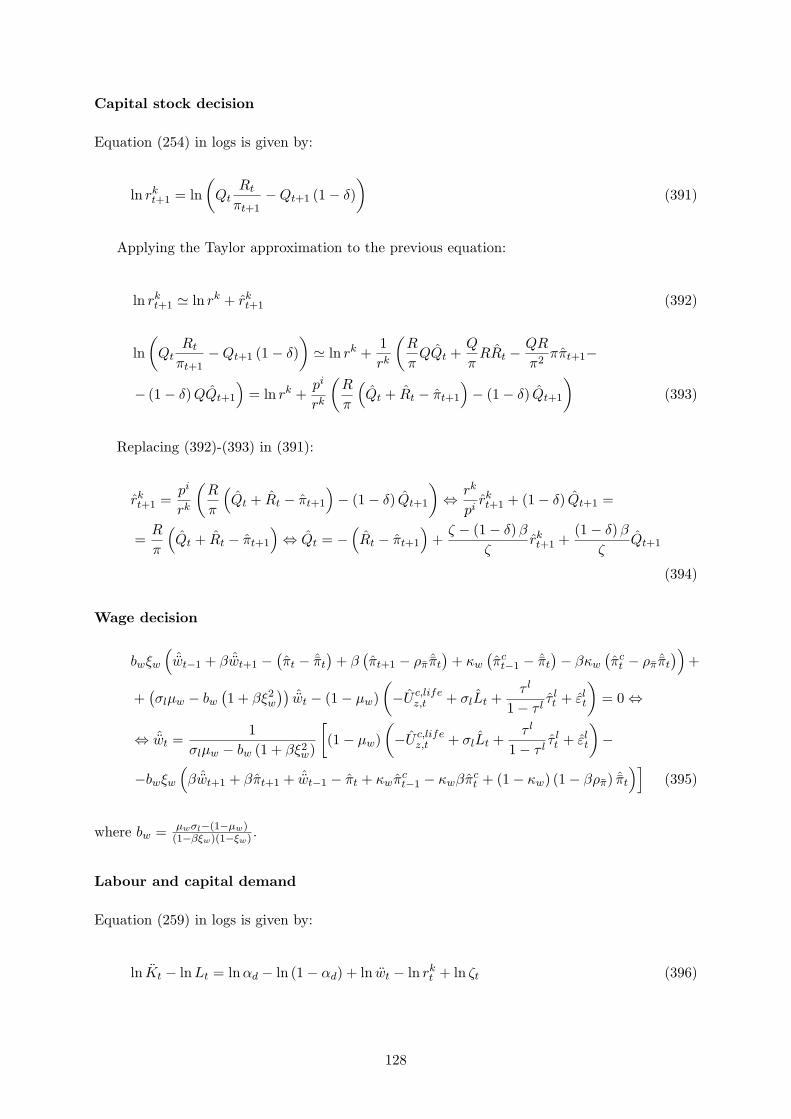
Capital stock decision
Equation (254) in logs is given by:
ln rkt+1 = ln
(Qt
Rt
πt+1−Qt+1 (1− δ)
)(391)
Applying the Taylor approximation to the previous equation:
ln rkt+1 ' ln rk + rk
t+1 (392)
ln(
QtRt
πt+1−Qt+1 (1− δ)
)' ln rk +
1rk
(R
πQQt +
Q
πRRt − QR
π2ππt+1−
− (1− δ) QQt+1
)= ln rk +
pi
rk
(R
π
(Qt + Rt − πt+1
)− (1− δ) Qt+1
)(393)
Replacing (392)-(393) in (391):
rkt+1 =
pi
rk
(R
π
(Qt + Rt − πt+1
)− (1− δ) Qt+1
)⇔ rk
pirkt+1 + (1− δ) Qt+1 =
=R
π
(Qt + Rt − πt+1
)⇔ Qt = −
(Rt − πt+1
)+
ζ − (1− δ) β
ζrkt+1 +
(1− δ) β
ζQt+1
(394)
Wage decision
bwξw
(ˆwt−1 + β ˆwt+1 −
(πt − ˆπt
)+ β
(πt+1 − ρπ ˆπt
)+ κw
(πc
t−1 − ˆπt
)− βκw
(πc
t − ρπ ˆπt
))+
+(σlµw − bw
(1 + βξ2
w
)) ˆwt − (1− µw)(−U c,life
z,t + σlLt +τ l
1− τ lτ lt + εl
t
)= 0 ⇔
⇔ ˆwt =1
σlµw − bw (1 + βξ2w)
[(1− µw)
(−U c,life
z,t + σlLt +τ l
1− τ lτ lt + εl
t
)−
−bwξw
(β ˆwt+1 + βπt+1 + ˆwt−1 − πt + κwπc
t−1 − κwβπct + (1− κw) (1− βρπ) ˆπt
)](395)
where bw = µwσl−(1−µw)(1−βξw)(1−ξw) .
Labour and capital demand
Equation (259) in logs is given by:
ln Kt − lnLt = ln αd − ln (1− αd) + ln wt − ln rkt + ln ζt (396)
128
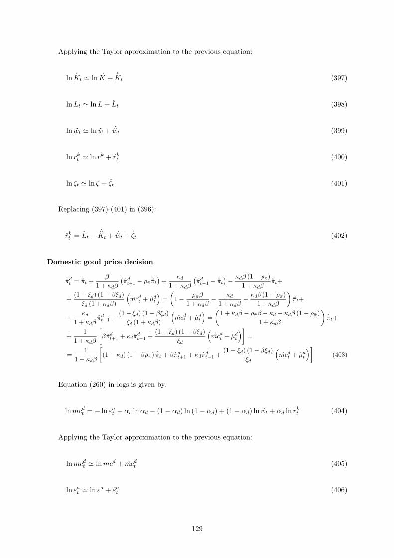
Applying the Taylor approximation to the previous equation:
ln Kt ' ln K + ˆKt (397)
ln Lt ' ln L + Lt (398)
ln wt ' ln w + ˆwt (399)
ln rkt ' ln rk + rk
t (400)
ln ζt ' ln ζ + ζt (401)
Replacing (397)-(401) in (396):
rkt = Lt − ˆKt + ˆwt + ζt (402)
Domestic good price decision
πdt = ˆπt +
β
1 + κdβ
(πd
t+1 − ρπ ˆπt
)+
κd
1 + κdβ
(πd
t−1 − ˆπt
)− κdβ (1− ρπ)1 + κdβ
ˆπt+
+(1− ξd) (1− βξd)
ξd (1 + κdβ)
(mcd
t + µdt
)=
(1− ρπβ
1 + κdβ− κd
1 + κdβ− κdβ (1− ρπ)
1 + κdβ
)ˆπt+
+κd
1 + κdβπd
t−1 +(1− ξd) (1− βξd)
ξd (1 + κdβ)
(mcd
t + µdt
)=
(1 + κdβ − ρπβ − κd − κdβ (1− ρπ)
1 + κdβ
)ˆπt+
+1
1 + κdβ
[βπd
t+1 + κdπdt−1 +
(1− ξd) (1− βξd)ξd
(mcd
t + µdt
)]=
=1
1 + κdβ
[(1− κd) (1− βρπ) ˆπt + βπd
t+1 + κdπdt−1 +
(1− ξd) (1− βξd)ξd
(mcd
t + µdt
)](403)
Equation (260) in logs is given by:
ln mcdt = − ln εa
t − αd ln αd − (1− αd) ln (1− αd) + (1− αd) ln wt + αd ln rkt (404)
Applying the Taylor approximation to the previous equation:
ln mcdt ' lnmcd + mcd
t (405)
ln εat ' ln εa + εa
t (406)
129
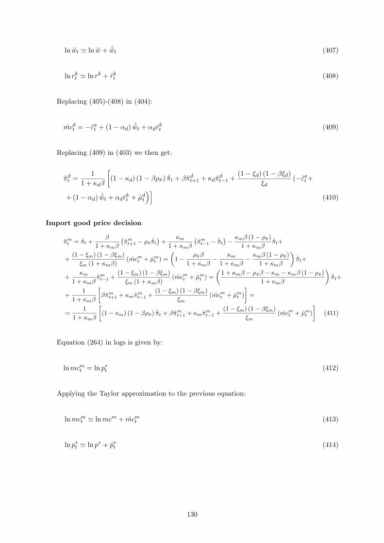
ln wt ' ln w + ˆwt (407)
ln rkt ' ln rk + rk
t (408)
Replacing (405)-(408) in (404):
mcdt = −εa
t + (1− αd) ˆwt + αdrkt (409)
Replacing (409) in (403) we then get:
πdt =
11 + κdβ
[(1− κd) (1− βρπ) ˆπt + βπd
t+1 + κdπdt−1 +
(1− ξd) (1− βξd)ξd
(−εat +
+(1− αd) ˆwt + αdrkt + µd
t
)](410)
Import good price decision
πmt = ˆπt +
β
1 + κmβ
(πm
t+1 − ρπ ˆπt
)+
κm
1 + κmβ
(πm
t−1 − ˆπt
)− κmβ (1− ρπ)1 + κmβ
ˆπt+
+(1− ξm) (1− βξm)
ξm (1 + κmβ)(mcm
t + µmt ) =
(1− ρπβ
1 + κmβ− κm
1 + κmβ− κmβ (1− ρπ)
1 + κmβ
)ˆπt+
+κm
1 + κmβπm
t−1 +(1− ξm) (1− βξm)
ξm (1 + κmβ)(mcm
t + µmt ) =
(1 + κmβ − ρπβ − κm − κmβ (1− ρπ)
1 + κmβ
)ˆπt+
+1
1 + κmβ
[βπm
t+1 + κmπmt−1 +
(1− ξm) (1− βξm)ξm
(mcmt + µm
t )]
=
=1
1 + κmβ
[(1− κm) (1− βρπ) ˆπt + βπm
t+1 + κmπmt−1 +
(1− ξm) (1− βξm)ξm
(mcmt + µm
t )]
(411)
Equation (264) in logs is given by:
ln mcmt = ln p∗t (412)
Applying the Taylor approximation to the previous equation:
ln mcmt ' lnmcm + mcm
t (413)
ln p∗t ' ln p∗ + p∗t (414)
130
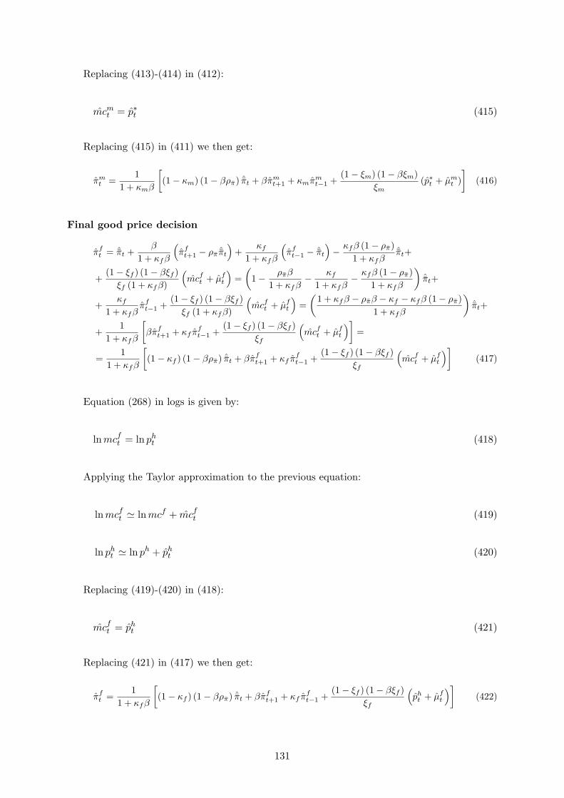
Replacing (413)-(414) in (412):
mcmt = p∗t (415)
Replacing (415) in (411) we then get:
πmt =
11 + κmβ
[(1− κm) (1− βρπ) ˆπt + βπm
t+1 + κmπmt−1 +
(1− ξm) (1− βξm)ξm
(p∗t + µmt )
](416)
Final good price decision
πft = ˆπt +
β
1 + κfβ
(πf
t+1 − ρπ ˆπt
)+
κf
1 + κfβ
(πf
t−1 − ˆπt
)− κfβ (1− ρπ)
1 + κfβˆπt+
+(1− ξf ) (1− βξf )
ξf (1 + κfβ)
(mcf
t + µft
)=
(1− ρπβ
1 + κfβ− κf
1 + κfβ− κfβ (1− ρπ)
1 + κfβ
)ˆπt+
+κf
1 + κfβπf
t−1 +(1− ξf ) (1− βξf )
ξf (1 + κfβ)
(mcf
t + µft
)=
(1 + κfβ − ρπβ − κf − κfβ (1− ρπ)
1 + κfβ
)ˆπt+
+1
1 + κfβ
[βπf
t+1 + κf πft−1 +
(1− ξf ) (1− βξf )ξf
(mcf
t + µft
)]=
=1
1 + κfβ
[(1− κf ) (1− βρπ) ˆπt + βπf
t+1 + κf πft−1 +
(1− ξf ) (1− βξf )ξf
(mcf
t + µft
)](417)
Equation (268) in logs is given by:
ln mcft = ln ph
t (418)
Applying the Taylor approximation to the previous equation:
ln mcft ' lnmcf + mcf
t (419)
ln pht ' ln ph + ph
t (420)
Replacing (419)-(420) in (418):
mcft = ph
t (421)
Replacing (421) in (417) we then get:
πft =
11 + κfβ
[(1− κf ) (1− βρπ) ˆπt + βπf
t+1 + κf πft−1 +
(1− ξf ) (1− βξf )ξf
(ph
t + µft
)](422)
131

We can then write:
πct =
11 + κcβ
[(1− κc) (1− βρπ) ˆπt + βπc
t+1 + κcπct−1 +
(1− ξc) (1− βξc)ξc
(ph
t + µct
)](423)
πit =
11 + κiβ
[(1− κi) (1− βρπ) ˆπt + βπi
t+1 + κiπit−1 +
(1− ξi) (1− βξi)ξi
(ph
t + µit
)](424)
πgt =
11 + κgβ
[(1− κg) (1− βρπ) ˆπt + βπg
t+1 + κgπgt−1 +
(1− ξg) (1− βξg)ξg
(ph
t + µgt
)](425)
πxt =
11 + κxβ
[(1− κx) (1− βρπ) ˆπt + βπx
t+1 + κxπxt−1 +
(1− ξx) (1− βξx)ξx
(ph
t + µxt
)](426)
Primary fiscal deficit
Equation (272) in logs is given by:
ln sgprimt = ln
(pg
t Gt + trt − τ ct pc
tCt − τ lt wtLt
)(427)
Applying the Taylor approximation to the previous equation:
ln sgprimt ' ln sgprim + ˆsgprim
t (428)
ln(pg
t Gt + trt − τ ct pc
tCt − τ lt wtLt
)' ln sgprim +
1sgprim
(pgG ˆGt + Gpgpg
t + tr ˆtrt−
−τ cpcC ˆCt − Cpcτ cτ ct − Cτ cpcpc
t − τ lwLLt − τ lLw ˆwt − wLτ lτ lt
)= ln sgprim+
+1
sgprim
(pgG
(ˆGt + pg
t
)+ tr ˆtrt − τ cpcC
(ˆCt + τ c
t + pct
)− τ lwL
(Lt + ˆwt + τ l
t
))(429)
Replacing (428)-(429) in (427):
ˆsgprimt =
1sgprim
(pgG
(ˆGt + pg
t
)+ tr ˆtrt − τ cpcC
(ˆCt + τ c
t + pct
)− τ lwL
(Lt + ˆwt + τ l
t
))(430)
Total fiscal deficit
Equation (273) in logs is given by:
ln sgtott = ln
(sgprim
t + (Rt−1 − 1)bt
πtζt
)(431)
132

Applying the Taylor approximation to the previous equation:
ln sgtott ' ln sgtot + ˆsgtot
t (432)
ln
(sgprim
t + (Rt−1 − 1)bt
πtζt
)' ln sgtot +
1sgtot
(sgprim ˆsgprim
t +R− 1
πζbˆbt−
−(R− 1) b
πζ2ζζt +
b
πζRRt−1 − (R− 1) b
ζπ2ππt
)= ln sgtot +
1sgtot
(sgprim ˆsgprim
t +
+b
ζπ
((R− 1)
(ˆbt − ζt − πt
)+ RRt−1
))(433)
Replacing (432)-(433) in (431):
ˆsgtott =
1sgtot
(sgprim ˆsgprim
t +b
ζπ
((R− 1)
(ˆbt − ζt − πt
)+ RRt−1
))(434)
Government’s budget constraint
Equation (274) in logs is given by:
ln bt+1 = ln
(bt
πtζt+ sgtot
t
)(435)
Applying the Taylor approximation to the previous equation:
ln bt+1 ' ln b + ˆbt+1 (436)
ln
(bt
πtζt+ sgtot
t
)' ln b +
1b
(1πζ
bˆbt − b
πζ2ζζt − b
ζπ2ππt + sgtot ˆsgtot
t
)= ln b +
1b×
×(
b
πζ
(ˆbt − ζt − πt
)+ sgtot ˆsgtot
t
)= ln b +
1πζ
(ˆbt − ζt − πt
)+
sgtot
b
1sgtot
(sgprim ˆsgprim
t +
+b
ζπ
((R− 1)
(ˆbt − ζt − πt
)+ RRt−1
))= ln b +
1πζ
(ˆbt − ζt − πt
)+
sgprim
bˆsgprim
t +
+1ζπ
((R− 1)
(ˆbt − ζt − πt
)+ RRt−1
)= ln b +
1πζ
(ˆbt − ζt − πt
)+
sgprim
b×
×(
1sgprim
(pgG
(ˆGt + pg
t
)+ tr ˆtrt − τ cpcC
(ˆCt + τ c
t + pct
)− τ lwL
(Lt + ˆwt + τ l
t
)))+
+1ζπ
((R− 1)
(ˆbt − ζt − πt
)+ RRt−1
)= ln b +
1b
(pgG
(ˆGt + pg
t
)+ tr ˆtrt−
−τ cpcC(
ˆCt + τ ct + pc
t
)− τ lwL
(Lt + ˆwt + τ l
t
))+
R
ζπ
(ˆbt − ζt − πt + Rt−1
)(437)
133
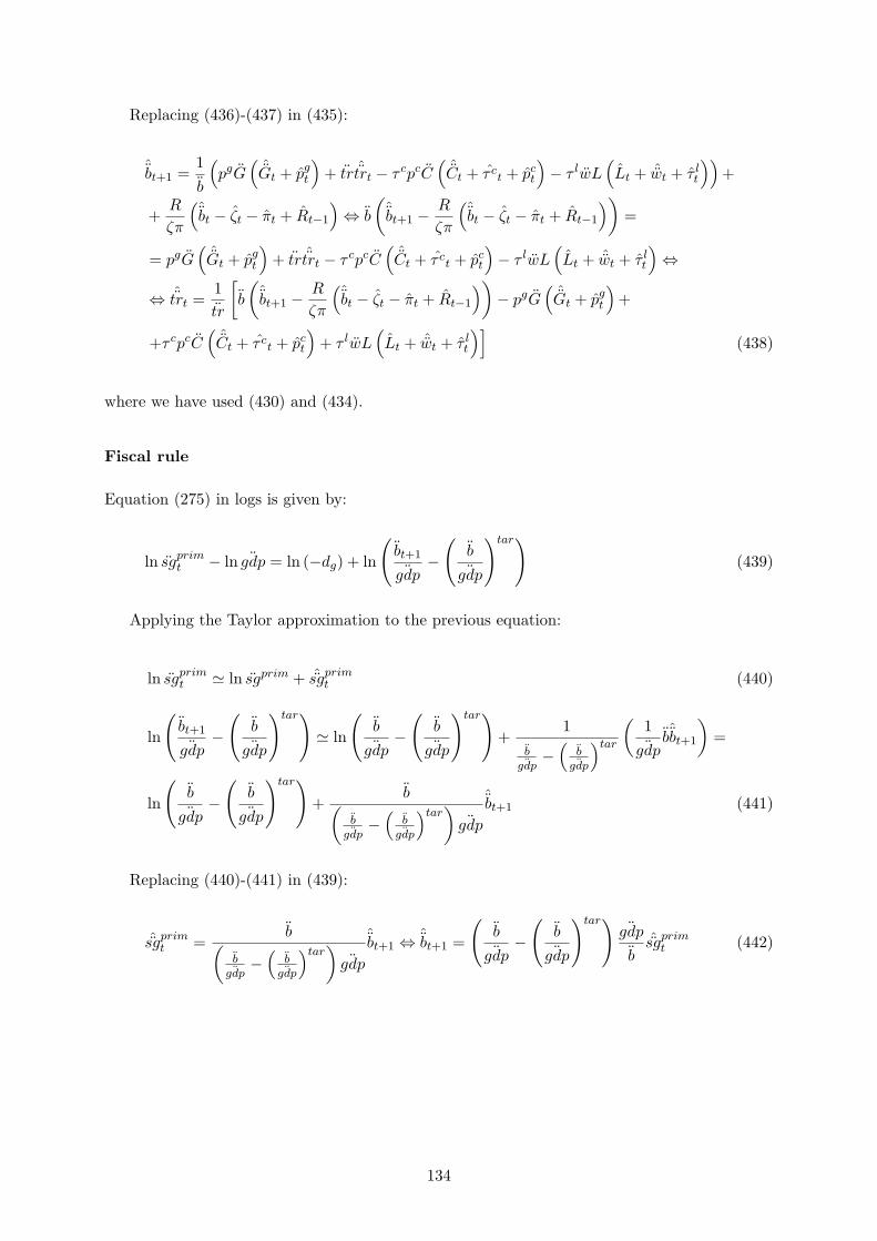
Replacing (436)-(437) in (435):
ˆbt+1 =
1b
(pgG
(ˆGt + pg
t
)+ tr ˆtrt − τ cpcC
(ˆCt + τ c
t + pct
)− τ lwL
(Lt + ˆwt + τ l
t
))+
+R
ζπ
(ˆbt − ζt − πt + Rt−1
)⇔ b
(ˆbt+1 − R
ζπ
(ˆbt − ζt − πt + Rt−1
))=
= pgG(
ˆGt + pgt
)+ tr ˆtrt − τ cpcC
(ˆCt + τ c
t + pct
)− τ lwL
(Lt + ˆwt + τ l
t
)⇔
⇔ ˆtrt =1tr
[b
(ˆbt+1 − R
ζπ
(ˆbt − ζt − πt + Rt−1
))− pgG
(ˆGt + pg
t
)+
+τ cpcC(
ˆCt + τ ct + pc
t
)+ τ lwL
(Lt + ˆwt + τ l
t
)](438)
where we have used (430) and (434).
Fiscal rule
Equation (275) in logs is given by:
ln sgprimt − ln ¨gdp = ln (−dg) + ln
(bt+1
¨gdp−
(b¨gdp
)tar)(439)
Applying the Taylor approximation to the previous equation:
ln sgprimt ' ln sgprim + ˆsgprim
t (440)
ln
(bt+1
¨gdp−
(b¨gdp
)tar)' ln
(b¨gdp−
(b¨gdp
)tar)+
1b¨gdp−
(b¨gdp
)tar
(1¨gdp
bˆbt+1
)=
ln
(b¨gdp−
(b¨gdp
)tar)+
b(b¨gdp−
(b¨gdp
)tar)
¨gdp
ˆbt+1 (441)
Replacing (440)-(441) in (439):
ˆsgprimt =
b(b¨gdp−
(b¨gdp
)tar)
¨gdp
ˆbt+1 ⇔ ˆ
bt+1 =
(b¨gdp−
(b¨gdp
)tar) ¨gdp
bˆsgprim
t (442)
134

Domestic good supply
Equation (276) in logs is given by:
ln Y dt =
µdt
µdt − 1
ln(
~pdt
pdt
)+ ln ~Y d
t (443)
Applying the Taylor approximation to the previous equation:
ln Y dt ' ln Y d + ˆY d
t (444)
ln(
~pdt
pdt
)' 0 (445)
ln ~Y dt ' ln ~Y d +
ˆ~Y d
t (446)
Replacing (444)-(446) in (443):
ˆY dt =
ˆ~Y d
t (447)
Equation (277) in logs is given by:
ln(
~Y dt + φd
)= ln εa
t + αd
(ln Kt − ln ζt
)+ (1− αd) lnLt (448)
Applying the Taylor approximation to the previous equation:
ln(
~Y dt + φd
)' ln
(~Y d + φd
)+
1~Y d + φd
~Y d ˆ~Y d
t (449)
ln εat ' ln εa + εa
t (450)
ln Kt ' ln K + ˆKt (451)
ln ζt ' ln ζ + ζt (452)
ln Lt ' ln L + Lt (453)
135
Replacing (449)-(453) in (448):
1~Y d + φd
~Y d ˆ~Y d
t = εat + αd
(ˆKt − ζt
)+ (1− αf ) Lt ⇔
ˆ~Y d
t =~Y d + φd
~Y d×
×(εat + αd
(ˆKt − ζt
)+ (1− αd)
ˆL)
=Y d + φd
Y d
(εat + αd
(ˆKt − ζt
)+ (1− αd)
ˆL)
(454)
where we have used (329).
Replacing (454) in (447):
ˆY dt =
Y d + φd
Y d
(εat + αd
(ˆKt − ζt
)+ (1− αd)
ˆL)
=Y d +
(µd − 1
)Y d
Y d×
×(εat + αd
(ˆKt − ζt
)+ (1− αd)
ˆL)
= µd(εat + αd
(ˆKt − ζt
)+ (1− αd)
ˆLt
)⇔
⇔ ˆLt =1
1− αd
( ˆY dt
µd− εa
t − αd
(ˆKt − ζt
))(455)
where we have used (335).
Aggregate wage and prices
Equation (283) in logs is given by:
ln pht = − 1
ϑhln
((1− ωh)
(pd
t
)−ϑh
+ ωh (pmt )−ϑh
)(456)
Applying the Taylor approximation to the previous equation:
ln pht ' ln ph + ph
t (457)
ln((1− ωh)
(pd
t
)−ϑh + ωh (pmt )−ϑh
)' ln ph +
1ph
(−ϑh (1− ωh)
(pd
)−ϑh−1pdpd
t−
−ϑhωh (pm)−ϑh−1pmpm
t
)= ln ph − 1
ph
(ϑh (1− ωh)
(pd
)−ϑhpd
t − ϑhωh (pm)−ϑh pmt
)(458)
Replacing (457)-(458) in (456):
pht = − 1
ϑh
(1ph
(−ϑh (1− ωh)
(pd
)−ϑh
pdt − ϑhωh (pm)−ϑh pm
t
))⇔
⇔ pht =
1ph
((1− ωh)
(pd
)−ϑh
pdt + ωh (pm)−ϑh pm
t
)(459)
136
Imports
Equation (284) in logs is given by:
ln Mt = lnωh − ln (1− ωh) + (ϑh + 1)(ln pd
t − ln pmt
)+ ln Y d
t (460)
Applying the Taylor approximation to the previous equation:
ln Mt ' ln M + ˆMt (461)
ln pdt ' ln pd + pd
t (462)
ln pmt ' ln pm + pm
t (463)
ln Y dt ' ln Y d + ˆY d
t (464)
Replacing (461)-(464) in (460):
ˆMt = (ϑh + 1)(pd
t − pmt
)+ ˆY d
t (465)
Exports
Equation (285) in logs is given by:
ln Xt = (ϑ∗ + 1) ln p∗t + ln ζ∗t + ln Y ∗t (466)
Applying the Taylor approximation to the previous equation:
ln Xt ' ln X + ˆXt (467)
ln p∗t ' ln p∗ + p∗t (468)
ln ζ∗t ' ln ζ∗ + ζ∗t (469)
ln Y ∗t ' ln Y ∗ + ˆY ∗
t (470)
137
Replacing (467)-(470) in (466):
ˆXt = (ϑ∗ + 1) p∗t + ζ∗t + ˆY ∗t (471)
Foreign bond market clearing condition
The linearisation of the foreign bond market equilibrium condition is performed in a slightly
different way. We apply the Taylor approximation on (286) directly, instead of its log and we
consider ˆb∗t = b∗t − b∗ instead of ˆ
b∗t = b∗t−b∗
b∗:
b∗ + ˆb∗t+1 = pxX ˆXt + Xpxpx
t − p∗M ˆMt − Mp∗p∗t + Φ(b∗, εφ
) b∗
πζR∗R∗
t−1 +R∗
πζ×
×(−Φ
(b∗, εφ
)b∗ + Φ
(b∗, εφ
)) ˆb∗t + R∗ b∗
πζΠ
(b∗, εφ
)εφεφ
t −R∗Φ(b∗, εφ
) b∗
π
1ζ2
ζζt−
−R∗Φ(b∗, εφ
) b∗
ζ
1π2
ππt = pxX(
ˆXt + pxt
)− M
(ˆMt + p∗t
)+
R∗
πζΦ
(b∗, εφ
) ˆb∗t =
= M(
ˆXt + pxt − ˆMt − p∗t
)+
R∗
πζˆb∗t ⇔ ˆ
b∗t+1 = M(
ˆXt + pxt − ˆMt − p∗t
)+
R
πζˆb∗t (472)
where we have used (348).
Aggregate resource constraint
Equation (287) in logs is given by:
ln Y dt = ln (1− ωh) + (ϑh + 1)
(ln ph
t − ln pdt
)+ ln
(Ct + It + Gt + Xt
)(473)
Applying the Taylor approximation to the previous equation:
ln Y dt ' ln Y d + ˆY d
t (474)
ln pht ' ln ph + ph
t (475)
ln pdt ' ln pd + pd
t (476)
ln(Ct + It + Gt + Xt
)= ln Y d +
1Y d
(C ˆCt + I ˆIt + G ˆGt + X ˆXt
)(477)
138
Replacing (474)-(475) in (473):
ˆY dt = (ϑh + 1)
(ph
t − pdt
)+
1Y d
(C ˆCt + I ˆIt + G ˆGt + X ˆXt
)(478)
GDP definition
Equation (288) in logs is given by:
ln ¨gdpt = ln(Ct + pg
t Gt + pitIt + px
t Xt − p∗t Mt
)(479)
Applying the Taylor approximation to the previous equation:
ln ¨gdpt ' ln ¨gdp + ˆgdpt (480)
ln(Ct + pg
t Gt + pitIt + px
t Xt − p∗t Mt
)' ln ¨gdp +
1¨gdp
(C ˆCt + pgG
(ˆGt + pg
t
)+
+piI(
ˆIt + pit
)+ pxX
(ˆXt + px
t
)− p∗M
(ˆMt + p∗t
))(481)
Replacing (480)-(481) in (479):
ˆgdpt =
1¨gdp
(C ˆCt + pgG
(ˆGt + pg
t
)+ piI
(ˆIt + pi
t
)+ pxX
(ˆXt + px
t
)− M
(ˆMt + p∗t
))(482)
Inflation identities
Equation (289) in logs is given by:
ln πwt − ln πt = ln wt − ln wt−1 + ln ζt (483)
Applying the Taylor approximation to the previous equation:
ln πwt ' ln πw + πw
t (484)
ln πt ' lnπ + πt (485)
ln wt ' ln w + ˆwt (486)
139
ln wt−1 ' ln w + ˆwt−1 (487)
ln ζt ' ln ζ + ζt (488)
Replacing (484)-(488) in (483):
πwt = ˆwt − ˆwt−1 + ζt + πt (489)
Equation (290) in logs is given by:
ln πdt − ln πt = ln pd
t − ln pdt−1 (490)
Applying the Taylor approximation to the previous equation:
ln πdt ' lnπd + πd
t (491)
ln πt ' lnπ + πt (492)
ln pdt ' ln pd + pd
t (493)
ln pdt−1 ' ln pd + pd
t−1 (494)
Replacing (491)-(494) in (490):
πdt = pd
t − pdt−1 + πt ⇔ pd
t = pdt−1 + πd
t − πt (495)
Equation (291) in logs is given by:
ln πmt − ln πt = ln pm
t − ln pmt−1 (496)
Applying the Taylor approximation to the previous equation:
ln πmt ' ln πm + πm
t (497)
ln πt ' lnπ + πt (498)
140
ln pmt ' ln pm + pm
t (499)
ln pmt−1 ' ln pm + pm
t−1 (500)
Replacing (497)-(500) in (496):
πmt = pm
t − pmt−1 + πt ⇔ pm
t = pmt−1 + πm
t − πt (501)
Equation (292) in logs is given by:
ln πft − lnπt = ln pf
t − ln pft−1 (502)
Applying the Taylor approximation to the previous equation:
ln πft ' lnπf + πf
t (503)
ln πt ' lnπ + πt (504)
ln pft ' ln pf + pf
t (505)
ln pft−1 ' ln pf + pf
t−1 (506)
Replacing (503)-(506) in (502):
πft = pf
t − pft−1 + πt ⇔ pf
t = pft−1 + πf
t − πt (507)
We can then write:
pct = pc
t−1 + πct − πt ⇔ πt = pc
t−1 + πct − pc
t (508)
pit = pi
t−1 + πit − πt (509)
pgt = pg
t−1 + πgt − πt (510)
pxt = px
t−1 + πxt − πt (511)
141
Equation (293) in logs is given by:
ln πht − ln πt = ln ph
t − ln pht−1 (512)
Applying the Taylor approximation to the previous equation:
ln πht ' ln πh + πh
t (513)
ln πt ' lnπ + πt (514)
ln pht ' ln ph + ph
t (515)
ln pht−1 ' ln ph + ph
t−1 (516)
Replacing (513)-(516) in (512):
πht − πt = ph
t − pht−1 ⇔ πh
t = πt + pht − ph
t−1 (517)
Equation (294) in logs is given by:
ln π∗t − lnπt = ln p∗t − ln p∗t−1 (518)
Applying the Taylor approximation to the previous equation:
ln π∗t ' lnπ∗ + π∗t (519)
ln πt ' lnπ + πt (520)
ln p∗t ' ln p∗ + p∗t (521)
ln p∗t−1 ' ln p∗ + p∗t−1 (522)
Replacing (519)-(522) in (518):
π∗t − πt = p∗t − p∗t−1 ⇔ p∗t = π∗t + p∗t−1 − πt (523)
142
Numeraire definition
Equation (295) in logs is given by:
0 = ln (1 + τ ct ) + ln pc
t (524)
Applying the Taylor approximation to the previous equation:
ln (1 + τ ct ) ' ln (1 + τ c) +
11 + τ c
τcτct (525)
ln pct ' ln pc
t + pct (526)
Replacing (525)-(526) in (524):
0 =τc
1 + τ cτ ct + pc
t ⇔ pct = − τc
1 + τ cτ ct (527)
Shocks
Equation (296) in logs is given by:
ln ξt = ln((1− ρξ) ξ + ρξξt−1 + ηξ,t
)(528)
Applying the Taylor approximation to the previous equation:
ln ξt ' ln ξ + ξt (529)
ln((1− ρξ) ξ + ρξξt−1 + ηξ,t
) ' ln((1− ρξ) ξ + ρξξ + ηξ
)+
1(1− ρξ) ξ + ρξξ + ηξ
×
×(ρξξξt−1 + (ηξ,t − ηξ)
)= ln ξ +
1ξ
(ρξ ξξt−1 + ηξ,t
)= ln ξ + ρξ ξt−1 +
ηξ,t
ξ(530)
Replacing (529)-(530) in (528):
ξt = ρξ ξt−1 +ηξ,t
ξ(531)
143

Collecting the necessary equations to solve the log-linearised dynamic model
Solving the system of equations composed by (364), (373), (381), (386), (390), (394), (395),
(402), (410), (416), (423), (424), (425), (426), (430), (434), (438), (442), (455), (459), (465),
(472), (482), (495), (501), (508), (509), (510), (511), (517), (523), (527) and (531) we get the
dynamic path of the following endogenous variables: ˆKt,ˆCt, U c
z,t, Rt,ˆIt, Qt, ˆwt, rk
t , πdt , πm
t , πct ,
πit, πg
t , πxt , ˆsgprim
t , ˆsgtott , ˆtrt,
ˆbt,
ˆLt, pht , ˆMt,
ˆXt,ˆb∗t ,
ˆY dt , ˆ
gdpt, pdt , pm
t , πt, pit, pg
t , pxt , πh
t , p∗t , pct
and the shocks.
144
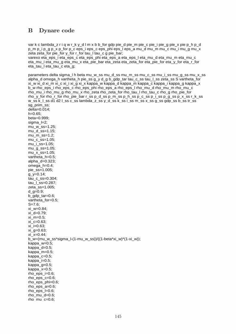
B Dynare code
var k c lambda_z r i q w r_k y_d l m x b b_for gdp pie_d pie_m pie_c pie_i pie_g pie_x pie p_h p_d p_m p_i p_g p_x p_for p_c eps_i eps_c eps_phi eps_l eps_a mu_d mu_m mu_c mu_i mu_g mu_x zeta zeta_for pie_for y_for r_for tau_l tau_c g pie_bar; varexo eta_eps_i eta_eps_c eta_eps_phi eta_eps_a eta_eps_l eta_mu_d eta_mu_m eta_mu_c eta_mu_i eta_mu_g eta_mu_x eta_pie_bar eta_zeta eta_zeta_for eta_pie_for eta_y_for eta_r_for eta_tau_l eta_tau_c eta_g; parameters delta sigma_l h beta mu_w_ss mu_d_ss mu_m_ss mu_c_ss mu_i_ss mu_g_ss mu_x_ss alpha_d omega_h vartheta_h pie_ss g_y d_g b_gdp_tar tau_c_ss tau_l_ss zeta_ss S vartheta_for xi_w xi_d xi_m xi_c xi_i xi_g xi_x kappa_w kappa_d kappa_m kappa_c kappa_i kappa_g kappa_x b_w rho_eps_i rho_eps_c rho_eps_phi rho_eps_a rho_eps_l rho_mu_d rho_mu_m rho_mu_c rho_mu_i rho_mu_g rho_mu_x rho_zeta rho_zeta_for rho_tau_l rho_tau_c rho_g rho_pie_for rho_y_for rho_r_for rho_pie_bar r_ss p_d_ss p_m_ss p_h_ss p_c_ss p_i_ss p_g_ss p_x_ss r_k_ss w_ss k_l_ss d1 d2 l_ss c_ss lambda_z_ss y_d_ss k_ss i_ss m_ss x_ss g_ss gdp_ss b_ss tr_ss sg_prim_ss; delta=0.014; h=0.65; beta=0.999; sigma_l=2; mu_w_ss=1.25; mu_d_ss=1.15; mu_m_ss=1.2; mu_c_ss=1.05; mu_i_ss=1.05; mu_g_ss=1.05; mu_x_ss=1.05; vartheta_h=0.5; alpha_d=0.323; omega_h=0.4; pie_ss=1.005; g_y=0.14; tau_c_ss=0.304; tau_l_ss=0.287; zeta_ss=1.005; d_g=0.9; b_gdp_tar=0.6; vartheta_for=0.5; S=7.6; xi_w=0.84; xi_d=0.79; xi_m=0.5; xi_c=0.63; xi_i=0.63; xi_g=0.63; xi_x=0.44; b_w=(mu_w_ss*sigma_l-(1-mu_w_ss))/((1-beta*xi_w)*(1-xi_w)); kappa_w=0.5; kappa_d=0.5; kappa_m=0.5; kappa_c=0.5; kappa_i=0.5; kappa_g=0.5; kappa_x=0.5; rho_eps_i=0.6; rho_eps_c=0.6; rho_eps_phi=0.6; rho_eps_a=0.6; rho_eps_l=0.6; rho_mu_d=0.6; rho_mu_c=0.6;
145

rho_mu_i=0.6; rho_mu_g=0.6; rho_mu_x=0.6; rho_mu_m=0.6; rho_zeta=0.6; rho_zeta_for=0.6; rho_tau_l=0.6; rho_tau_c=0.6; rho_g=0.6; rho_pie_for=0.6; rho_y_for=0.6; rho_r_for=0.6; rho_pie_bar=0.6; r_ss=(pie_ss*zeta_ss)/beta; p_c_ss=1/(1+tau_c_ss); p_m_ss=mu_m_ss; p_h_ss=p_c_ss/mu_c_ss; p_i_ss=mu_i_ss*p_h_ss; p_g_ss=mu_g_ss*p_h_ss; p_x_ss=mu_x_ss*p_h_ss; p_d_ss=((p_h_ss^(-vartheta_h)-omega_h*(p_m_ss^(-vartheta_h)))/(1-omega_h))^(-1/vartheta_h); r_k_ss=p_i_ss*(zeta_ss/beta-(1-delta)); w_ss=(p_d_ss/(mu_d_ss*r_k_ss^alpha_d)*alpha_d^alpha_d*(1-alpha_d)^(1-alpha_d))^(1/(1-alpha_d)); k_l_ss=alpha_d/(1-alpha_d)*(zeta_ss*w_ss)/r_k_ss; d1=(w_ss/mu_w_ss*(1-tau_l_ss)*(zeta_ss-beta*h)/(zeta_ss-h)*zeta_ss)^(1/sigma_l); d2=1/(1-omega_h)*(p_d_ss/p_h_ss)^(vartheta_h+1)*(1-g_y-1/p_x_ss*omega_h/(1-omega_h)*(p_d_ss/p_m_ss)^(vartheta_h+1))*1/mu_d_ss*(1/zeta_ss*k_l_ss)^alpha_d-(1-(1-delta)/zeta_ss)*k_l_ss; l_ss=(d1^sigma_l/d2)^(1/(sigma_l+1)); c_ss=d2*l_ss; lambda_z_ss=(zeta_ss-beta*h)/((zeta_ss-h)*c_ss); y_d_ss=1/mu_d_ss*(1/zeta_ss)^alpha_d*k_l_ss^alpha_d*l_ss; m_ss=omega_h/(1-omega_h)*(p_d_ss/p_m_ss)^(vartheta_h+1)*y_d_ss; k_ss=k_l_ss*l_ss; i_ss=(1-(1-delta)/zeta_ss)*k_ss; x_ss=m_ss/p_x_ss; g_ss=g_y*y_d_ss; gdp_ss=c_ss+p_i_ss*i_ss+p_g_ss*g_ss; b_ss=d_g*pie_ss*zeta_ss/(d_g*pie_ss*zeta_ss+pie_ss*zeta_ss-r_ss)*b_gdp_tar*gdp_ss; b_gdp_ss=b_ss/gdp_ss; tr_ss=(1-r_ss/(pie_ss*zeta_ss))*b_ss-p_g_ss*g_ss+tau_c_ss*p_c_ss*c_ss+tau_l_ss*w_ss*l_ss; sg_prim_ss=p_g_ss*g_ss+tr_ss-tau_c_ss*p_c_ss*c_ss-tau_l_ss*w_ss*l_ss; model(linear); k=(1-delta)/zeta_ss*(k(-1)-zeta)+(1-(1-delta)/zeta_ss)*(eps_i+i); c=1/(zeta_ss^2+beta*h^2)*(zeta_ss*h*c(-1)-zeta_ss*h*zeta-beta*h*(zeta_ss-h)*eps_c(+1)+beta*h*zeta_ss*c(+1)+beta*h*zeta_ss*zeta(+1)+zeta_ss*(zeta_ss-h)*eps_c-(zeta_ss-beta*h)*(zeta_ss-h)*lambda_z); lambda_z=lambda_z(+1)+r-pie(+1)-zeta(+1); r=r_for-b_for+eps_phi; i=1/(1+beta)*((q+eps_i-p_i)/(S*zeta_ss^2)+i(-1)-zeta+beta*i(+1)+beta*zeta(+1)); q=-(r-pie(+1))+(zeta_ss-(1-delta))/zeta_ss*r_k(+1)+(1-delta)*beta/zeta_ss*q(+1); w=1/(sigma_l*mu_w_ss-b_w*(1+beta*xi_w^2))*((1-mu_w_ss)*(-lambda_z+sigma_l*l+tau_l_ss/(1-tau_l_ss)*tau_l+eps_l)-b_w*xi_w*(beta*(w(+1)+pie(+1))+w(-1)-pie+kappa_w*(pie(-1)-beta*pie)+(1-kappa_w)*(1-beta*rho_pie_bar)*pie_bar)); r_k=l-k(-1)+zeta+w; pie_d=1/(1+kappa_d*beta)*((1-kappa_d)*(1-beta*rho_pie_bar)*pie_bar+beta*pie_d(+1)+kappa_d*pie_d(-1)+(1-xi_d)*(1-beta*xi_d)/xi_d*(-eps_a+(1-alpha_d)*w+alpha_d*r_k+mu_d));
146

pie_m=1/(1+kappa_m*beta)*((1-kappa_m)*(1-beta*rho_pie_bar)*pie_bar+beta*pie_m(+1)+kappa_m*pie_m(-1)+(1-xi_m)*(1-beta*xi_m)/xi_m*(p_for+mu_m)); pie_c=1/(1+kappa_c*beta)*((1-kappa_c)*(1-beta*rho_pie_bar)*pie_bar+beta*pie_c(+1)+kappa_c*pie_c(-1)+(1-xi_c)*(1-beta*xi_c)/xi_c*(p_h+mu_c)); pie_i=1/(1+kappa_i*beta)*((1-kappa_i)*(1-beta*rho_pie_bar)*pie_bar+beta*pie_i(+1)+kappa_i*pie_i(-1)+(1-xi_i)*(1-beta*xi_i)/xi_i*(p_h+mu_i)); pie_g=1/(1+kappa_g*beta)*((1-kappa_g)*(1-beta*rho_pie_bar)*pie_bar+beta*pie_g(+1)+kappa_g*pie_g(-1)+(1-xi_g)*(1-beta*xi_g)/xi_g*(p_h+mu_g)); pie_x=1/(1+kappa_x*beta)*((1-kappa_x)*(1-beta*rho_pie_bar)*pie_bar+beta*pie_x(+1)+kappa_x*pie_x(-1)+(1-xi_x)*(1-beta*xi_x)/xi_x*(p_h+mu_x)); l=1/(1-alpha_d)*(y_d/mu_d_ss-eps_a-alpha_d*(k(-1)-zeta)); x=(vartheta_for+1)*p_for+zeta_for+y_for; m=(vartheta_h+1)*(p_d-p_m)+y_d; y_d=(vartheta_h+1)*(p_h-p_d)+1/y_d_ss*(c_ss*c+i_ss*i+g_ss*g+x_ss*x); b=(b_ss/gdp_ss-b_gdp_tar)*gdp_ss/b_ss*((1/sg_prim_ss)*(p_g_ss*g_ss*(g+p_g)+tr_ss*(1/tr_ss*(b_ss*(b-r_ss/(pie_ss*zeta_ss)*(b(-1)-zeta-pie+r(-1)))-p_g_ss*g_ss*(g+p_g)+tau_c_ss*p_c_ss*c_ss*(c+tau_c+p_c)+tau_l_ss*w_ss*l_ss*(l+w+tau_l)))-tau_c_ss*p_c_ss*c_ss*(c+tau_c+p_c)-tau_l_ss*w_ss*l_ss*(l+w+tau_l))); b_for=m_ss*(x+p_x-m-p_for)+r_ss/(pie_ss*zeta_ss)*b_for(-1); gdp=1/gdp_ss*(c_ss*c+p_g_ss*g_ss*(g+p_g)+p_i_ss*i_ss*(i+p_i)+p_x_ss*x_ss*(x+p_x)-m_ss*(m+p_for)); p_c=-tau_c_ss/(1+tau_c_ss)*tau_c; pie=p_c(-1)+pie_c-p_c; p_h=1/p_h_ss*((1-omega_h)*p_d_ss^(-vartheta_h)*p_d+omega_h*p_m_ss^(-vartheta_h)*p_m); p_d=pie_d+p_d(-1)-pie; p_m=pie_m+p_m(-1)-pie; p_i=pie_i+p_i(-1)-pie; p_g=pie_g+p_g(-1)-pie; p_x=pie_x+p_x(-1)-pie; p_for=pie_for+p_for(-1)-pie; eps_i=rho_eps_i*eps_i(-1)+eta_eps_i; eps_c=rho_eps_c*eps_c(-1)+eta_eps_c; eps_phi=rho_eps_phi*eps_phi(-1)+eta_eps_phi; eps_l=rho_eps_l*eps_l(-1)+eta_eps_l; eps_a=rho_eps_a*eps_a(-1)+eta_eps_a; mu_d=rho_mu_d*mu_d(-1)+eta_mu_d/mu_d_ss; mu_m=rho_mu_m*mu_m(-1)+eta_mu_m/mu_m_ss; mu_c=rho_mu_c*mu_c(-1)+eta_mu_c/mu_c_ss; mu_i=rho_mu_i*mu_i(-1)+eta_mu_i/mu_i_ss; mu_g=rho_mu_g*mu_g(-1)+eta_mu_g/mu_g_ss; mu_x=rho_mu_x*mu_x(-1)+eta_mu_x/mu_x_ss; zeta=rho_zeta*zeta(-1)+eta_zeta/zeta_ss; zeta_for=rho_zeta_for*zeta_for(-1)+eta_zeta_for; pie_bar=rho_pie_bar*pie_bar(-1)+eta_pie_bar/pie_ss; pie_for=rho_pie_for*pie_for(-1)+eta_pie_for/pie_ss; y_for=rho_y_for*y_for(-1)+eta_y_for; r_for=rho_r_for*r_for(-1)+eta_r_for/r_ss; tau_l=rho_tau_l*tau_l(-1)+eta_tau_l/tau_l_ss; tau_c=rho_tau_c*tau_c(-1)+eta_tau_c/tau_c_ss; g=rho_g*g(-1)+eta_g/g_ss; end; initval; k=0; c=0;
147

lambda_z=0; r=0; i=0; q=0; w=0; r_k=0; l=0; x=0; m=0; y_d=0; b=0; b_for=0; gdp=0; pie_d=0; pie_m=0; pie_c=0; pie_i=0; pie_g=0; pie_x=0; p_c=0; pie=0; p_h=0; p_d=0; p_m=0; p_i=0; p_g=0; p_x=0; p_for=0; eps_i=0; eps_c=0; eps_phi=0; eps_l=0; eps_a=0; mu_d=0; mu_m=0; mu_c=0; mu_i=0; mu_g=0; mu_x=0; zeta=0; zeta_for=0; pie_bar=0; pie_for=0; y_for=0; r_for=0; tau_l=0; tau_c=0; g=0; eta_eps_i=0; eta_eps_c=0; eta_eps_phi=0; eta_eps_a=0; eta_eps_l=0; eta_mu_d=0; eta_mu_m=0; eta_mu_c=0; eta_mu_i=0; eta_mu_g=0; eta_mu_x=0; eta_pie_bar=0;
148

eta_zeta=0; eta_zeta_for=0; eta_pie_for=0; eta_y_for=0; eta_r_for=0; eta_tau_l=0; eta_tau_c=0; eta_g=0; end; steady; check; shocks; var eta_eps_i; stderr 0.15; var eta_eps_c; stderr 0.15; var eta_eps_phi; stderr 0.02; var eta_eps_a; stderr 0.02; var eta_eps_l; stderr 0.15; var eta_mu_d; stderr 0.15; var eta_mu_c; stderr 0.15; var eta_mu_i; stderr 0.15; var eta_mu_g; stderr 0.15; var eta_mu_x; stderr 0.15; var eta_mu_m; stderr 0.15; var eta_zeta; stderr 0.15; var eta_zeta_for; stderr 0.15; var eta_tau_l; stderr 0.15; var eta_tau_c; stderr 0.02; var eta_g; stderr 0.02; var eta_pie_for; stderr 0.02; var eta_y_for; stderr 0.02; var eta_r_for; stderr 0.02; var eta_pie_bar; stderr 0.02; end; estimated_params; mu_w_ss,inv_gamma_pdf,1.25,0.2; mu_d_ss,inv_gamma_pdf,1.15,0.2; mu_m_ss,inv_gamma_pdf,1.2,0.2; mu_c_ss,inv_gamma_pdf,1.05,0.2; mu_i_ss,inv_gamma_pdf,1.05,0.2; mu_g_ss,inv_gamma_pdf,1.05,0.2; mu_x_ss,inv_gamma_pdf,1.05,0.2; vartheta_h,inv_gamma_pdf,0.5,0.1; omega_h,beta_pdf,0.4,0.1; vartheta_for,inv_gamma_pdf,0.5,0.1; S,normal_pdf,7.6,1.5; xi_w,beta_pdf,0.84,0.1; xi_d,beta_pdf,0.79,0.1; xi_i,beta_pdf,0.63,0.1; xi_g,beta_pdf,0.63,0.1; xi_x,beta_pdf,0.44,0.1; kappa_w,beta_pdf,0.5,0.1; kappa_d,beta_pdf,0.5,0.1; kappa_m,beta_pdf,0.5,0.1; kappa_c,beta_pdf,0.5,0.1; kappa_i,beta_pdf,0.5,0.1; kappa_g,beta_pdf,0.5,0.1;
149
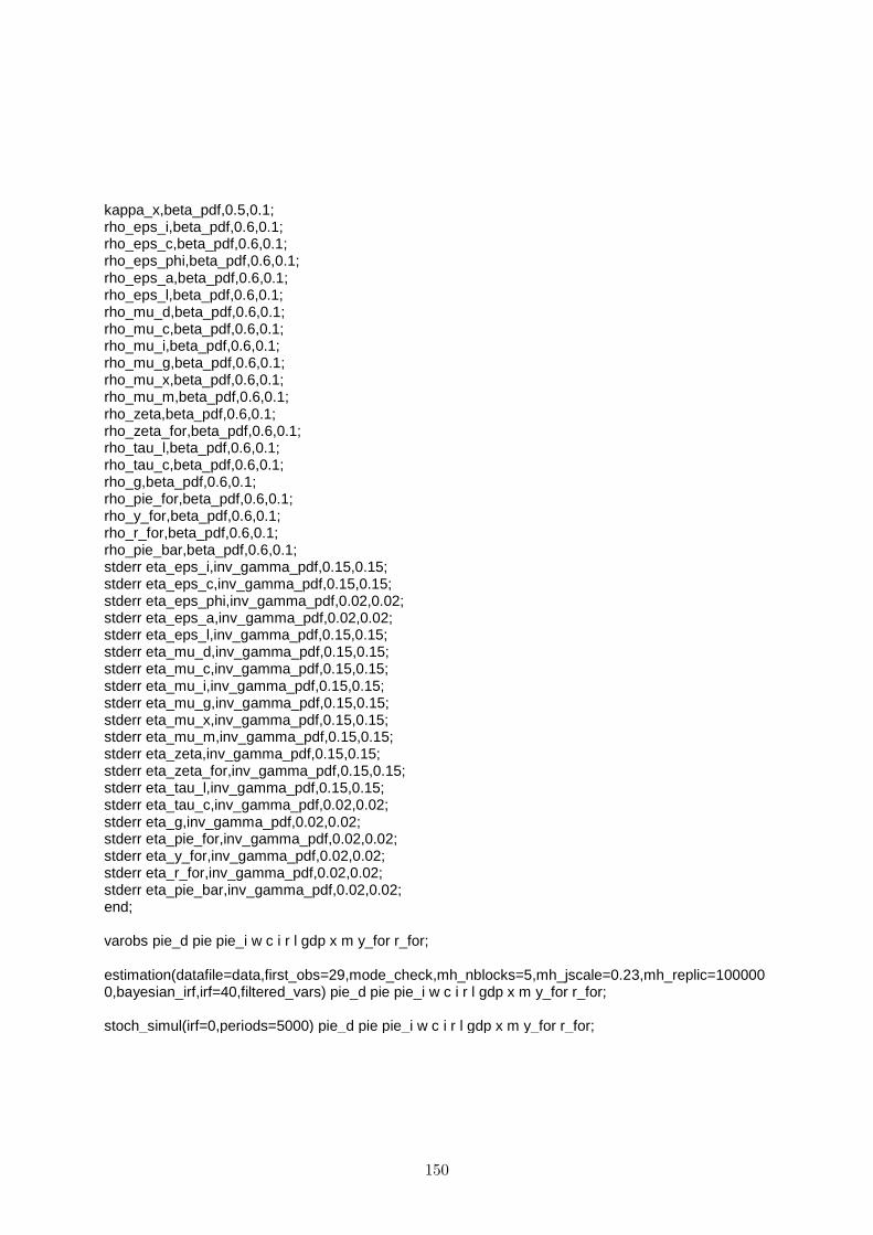
kappa_x,beta_pdf,0.5,0.1; rho_eps_i,beta_pdf,0.6,0.1; rho_eps_c,beta_pdf,0.6,0.1; rho_eps_phi,beta_pdf,0.6,0.1; rho_eps_a,beta_pdf,0.6,0.1; rho_eps_l,beta_pdf,0.6,0.1; rho_mu_d,beta_pdf,0.6,0.1; rho_mu_c,beta_pdf,0.6,0.1; rho_mu_i,beta_pdf,0.6,0.1; rho_mu_g,beta_pdf,0.6,0.1; rho_mu_x,beta_pdf,0.6,0.1; rho_mu_m,beta_pdf,0.6,0.1; rho_zeta,beta_pdf,0.6,0.1; rho_zeta_for,beta_pdf,0.6,0.1; rho_tau_l,beta_pdf,0.6,0.1; rho_tau_c,beta_pdf,0.6,0.1; rho_g,beta_pdf,0.6,0.1; rho_pie_for,beta_pdf,0.6,0.1; rho_y_for,beta_pdf,0.6,0.1; rho_r_for,beta_pdf,0.6,0.1; rho_pie_bar,beta_pdf,0.6,0.1; stderr eta_eps_i,inv_gamma_pdf,0.15,0.15; stderr eta_eps_c,inv_gamma_pdf,0.15,0.15; stderr eta_eps_phi,inv_gamma_pdf,0.02,0.02; stderr eta_eps_a,inv_gamma_pdf,0.02,0.02; stderr eta_eps_l,inv_gamma_pdf,0.15,0.15; stderr eta_mu_d,inv_gamma_pdf,0.15,0.15; stderr eta_mu_c,inv_gamma_pdf,0.15,0.15; stderr eta_mu_i,inv_gamma_pdf,0.15,0.15; stderr eta_mu_g,inv_gamma_pdf,0.15,0.15; stderr eta_mu_x,inv_gamma_pdf,0.15,0.15; stderr eta_mu_m,inv_gamma_pdf,0.15,0.15; stderr eta_zeta,inv_gamma_pdf,0.15,0.15; stderr eta_zeta_for,inv_gamma_pdf,0.15,0.15; stderr eta_tau_l,inv_gamma_pdf,0.15,0.15; stderr eta_tau_c,inv_gamma_pdf,0.02,0.02; stderr eta_g,inv_gamma_pdf,0.02,0.02; stderr eta_pie_for,inv_gamma_pdf,0.02,0.02; stderr eta_y_for,inv_gamma_pdf,0.02,0.02; stderr eta_r_for,inv_gamma_pdf,0.02,0.02; stderr eta_pie_bar,inv_gamma_pdf,0.02,0.02; end; varobs pie_d pie pie_i w c i r l gdp x m y_for r_for; estimation(datafile=data,first_obs=29,mode_check,mh_nblocks=5,mh_jscale=0.23,mh_replic=1000000,bayesian_irf,irf=40,filtered_vars) pie_d pie pie_i w c i r l gdp x m y_for r_for; stoch_simul(irf=0,periods=5000) pie_d pie pie_i w c i r l gdp x m y_for r_for;
150
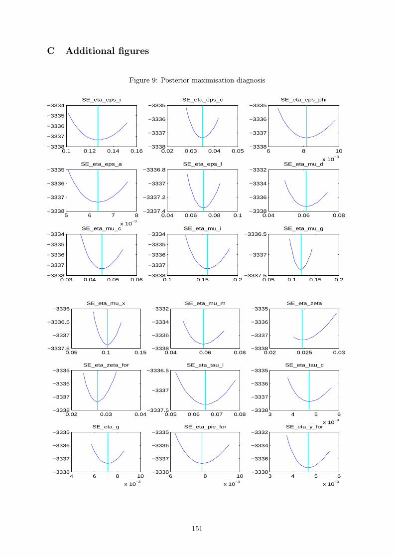
C Additional figures
Figure 9: Posterior maximisation diagnosis
0.1 0.12 0.14 0.16−3338
−3337
−3336
−3335
−3334SE_eta_eps_i
0.02 0.03 0.04 0.05−3338
−3337
−3336
−3335SE_eta_eps_c
6 8 10
x 10−3
−3338
−3337
−3336
−3335SE_eta_eps_phi
5 6 7 8
x 10−3
−3338
−3337
−3336
−3335SE_eta_eps_a
0.04 0.06 0.08 0.1−3337.4
−3337.2
−3337
−3336.8SE_eta_eps_l
0.04 0.06 0.08−3338
−3336
−3334
−3332SE_eta_mu_d
0.03 0.04 0.05 0.06−3338
−3337
−3336
−3335
−3334SE_eta_mu_c
0.1 0.15 0.2−3338
−3337
−3336
−3335
−3334SE_eta_mu_i
0.05 0.1 0.15 0.2−3337.5
−3337
−3336.5SE_eta_mu_g
0.05 0.1 0.15−3337.5
−3337
−3336.5
−3336SE_eta_mu_x
0.04 0.06 0.08−3338
−3336
−3334
−3332SE_eta_mu_m
0.02 0.025 0.03−3338
−3337
−3336
−3335SE_eta_zeta
0.02 0.03 0.04−3338
−3337
−3336
−3335SE_eta_zeta_for
0.05 0.06 0.07 0.08−3337.5
−3337
−3336.5SE_eta_tau_l
3 4 5 6
x 10−3
−3338
−3337
−3336
−3335SE_eta_tau_c
4 6 8 10
x 10−3
−3338
−3337
−3336
−3335SE_eta_g
6 8 10
x 10−3
−3338
−3337
−3336
−3335SE_eta_pie_for
3 4 5 6
x 10−3
−3338
−3336
−3334
−3332SE_eta_y_for
151
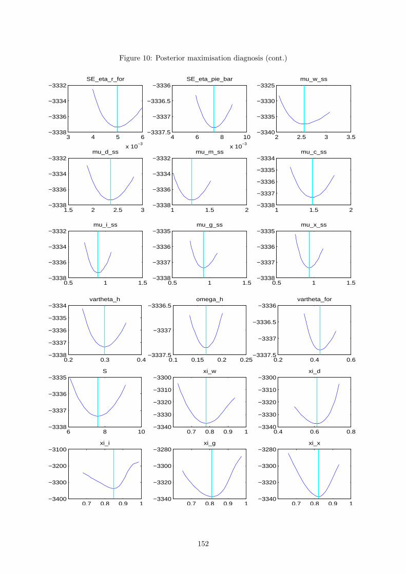
Figure 10: Posterior maximisation diagnosis (cont.)
3 4 5 6
x 10−3
−3338
−3336
−3334
−3332SE_eta_r_for
4 6 8 10
x 10−3
−3337.5
−3337
−3336.5
−3336SE_eta_pie_bar
2 2.5 3 3.5−3340
−3335
−3330
−3325mu_w_ss
1.5 2 2.5 3−3338
−3336
−3334
−3332mu_d_ss
1 1.5 2−3338
−3336
−3334
−3332mu_m_ss
1 1.5 2−3338
−3337
−3336
−3335
−3334mu_c_ss
0.5 1 1.5−3338
−3336
−3334
−3332mu_i_ss
0.5 1 1.5−3338
−3337
−3336
−3335mu_g_ss
0.5 1 1.5−3338
−3337
−3336
−3335mu_x_ss
0.2 0.3 0.4−3338
−3337
−3336
−3335
−3334vartheta_h
0.1 0.15 0.2 0.25−3337.5
−3337
−3336.5omega_h
0.2 0.4 0.6−3337.5
−3337
−3336.5
−3336vartheta_for
6 8 10−3338
−3337
−3336
−3335S
0.7 0.8 0.9 1−3340
−3330
−3320
−3310
−3300xi_w
0.4 0.6 0.8−3340
−3330
−3320
−3310
−3300xi_d
0.7 0.8 0.9 1−3400
−3300
−3200
−3100xi_i
0.7 0.8 0.9 1−3340
−3320
−3300
−3280xi_g
0.7 0.8 0.9 1−3340
−3320
−3300
−3280xi_x
152

Figure 11: Posterior maximisation diagnosis (cont.)
0.4 0.6 0.8−3338
−3337
−3336
−3335kappa_w
0.35 0.4 0.45 0.5−3337.5
−3337
−3336.5
−3336kappa_d
0.2 0.3 0.4−3337.4
−3337.2
−3337
−3336.8kappa_m
0.2 0.4 0.6−3337.4
−3337.2
−3337
−3336.8kappa_c
0.2 0.3 0.4−3337.4
−3337.2
−3337
−3336.8kappa_i
0.2 0.4 0.6−3337.5
−3337
−3336.5kappa_g
0.2 0.4 0.6−3337.5
−3337
−3336.5kappa_x
0.2 0.4 0.6−3337.5
−3337
−3336.5
−3336rho_eps_i
0.4 0.6 0.8−3337.5
−3337
−3336.5rho_eps_c
0.7 0.8 0.9 1−3338
−3336
−3334
−3332rho_eps_phi
0.7 0.8 0.9 1−3340
−3335
−3330
−3325
−3320rho_eps_a
0.4 0.6 0.8−3337.5
−3337
−3336.5
−3336rho_eps_l
0.4 0.6 0.8 1−3340
−3335
−3330rho_mu_d
0.4 0.6 0.8 1−3340
−3335
−3330
−3325
−3320rho_mu_c
0.4 0.6 0.8−3338
−3336
−3334
−3332rho_mu_i
0.4 0.6 0.8−3340
−3335
−3330rho_mu_g
0.4 0.6 0.8−3340
−3335
−3330rho_mu_x
0.2 0.3 0.4 0.5−3337.5
−3337
−3336.5rho_mu_m
153
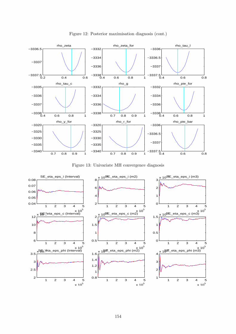
Figure 12: Posterior maximisation diagnosis (cont.)
0.2 0.4 0.6−3337.5
−3337
−3336.5rho_zeta
0.4 0.6 0.8 1−3338
−3336
−3334
−3332rho_zeta_for
0.4 0.6 0.8−3337.5
−3337
−3336.5
−3336rho_tau_l
0.4 0.6 0.8 1−3338
−3337
−3336
−3335rho_tau_c
0.7 0.8 0.9 1−3338
−3336
−3334
−3332rho_g
0.4 0.6 0.8 1−3338
−3336
−3334
−3332rho_pie_for
0.7 0.8 0.9 1−3340
−3335
−3330
−3325
−3320rho_y_for
0.7 0.8 0.9 1−3340
−3335
−3330
−3325
−3320rho_r_for
0.4 0.6 0.8−3337.5
−3337
−3336.5
−3336rho_pie_bar
Figure 13: Univariate MH convergence diagnosis
1 2 3 4 5
x 105
0.04
0.05
0.06
0.07
0.08SE_eta_eps_i (Interval)
1 2 3 4 5
x 105
2
4
6
8x 10
−4SE_eta_eps_i (m2)
1 2 3 4 5
x 105
0
1
2
3x 10
−5SE_eta_eps_i (m3)
1 2 3 4 5
x 105
6
8
10
12x 10
−3SE_eta_eps_c (Interval)
1 2 3 4 5
x 105
0.5
1
1.5
2x 10
−5SE_eta_eps_c (m2)
1 2 3 4 5
x 105
0
0.5
1
1.5x 10
−7SE_eta_eps_c (m3)
1 2 3 4 5
x 105
2
2.5
3
3.5x 10
−3SE_eta_eps_phi (Interval)
1 2 3 4 5
x 105
0.8
1
1.2
1.4
1.6x 10
−6SE_eta_eps_phi (m2)
1 2 3 4 5
x 105
1
2
3
4x 10
−9SE_eta_eps_phi (m3)
154
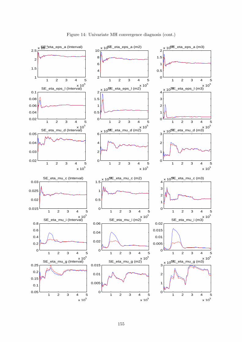
Figure 14: Univariate MH convergence diagnosis (cont.)
1 2 3 4 5
x 105
1
1.5
2
2.5x 10
−3SE_eta_eps_a (Interval)
1 2 3 4 5
x 105
2
4
6
8
10x 10
−7SE_eta_eps_a (m2)
1 2 3 4 5
x 105
0
0.5
1
1.5
2x 10
−9SE_eta_eps_a (m3)
1 2 3 4 5
x 105
0.02
0.04
0.06
0.08
0.1SE_eta_eps_l (Interval)
1 2 3 4 5
x 105
0
0.5
1
1.5
2x 10
−3SE_eta_eps_l (m2)
1 2 3 4 5
x 105
0
1
2
3
4x 10
−4SE_eta_eps_l (m3)
1 2 3 4 5
x 105
0.02
0.03
0.04
0.05SE_eta_mu_d (Interval)
1 2 3 4 5
x 105
0
2
4
6x 10
−4SE_eta_mu_d (m2)
1 2 3 4 5
x 105
0
1
2
3x 10
−5SE_eta_mu_d (m3)
1 2 3 4 5
x 105
0.015
0.02
0.025
0.03SE_eta_mu_c (Interval)
1 2 3 4 5
x 105
0
0.5
1
1.5x 10
−4SE_eta_mu_c (m2)
1 2 3 4 5
x 105
0
1
2
3
4x 10
−6SE_eta_mu_c (m3)
1 2 3 4 5
x 105
0
0.2
0.4
0.6
0.8SE_eta_mu_i (Interval)
1 2 3 4 5
x 105
0
0.02
0.04
0.06SE_eta_mu_i (m2)
1 2 3 4 5
x 105
0
0.005
0.01
0.015
0.02SE_eta_mu_i (m3)
1 2 3 4 5
x 105
0.05
0.1
0.15
0.2
0.25SE_eta_mu_g (Interval)
1 2 3 4 5
x 105
0
0.005
0.01
0.015SE_eta_mu_g (m2)
1 2 3 4 5
x 105
0
1
2
3x 10
−3SE_eta_mu_g (m3)
155

Figure 15: Univariate MH convergence diagnosis (cont.)
1 2 3 4 5
x 105
0.05
0.1
0.15
0.2
0.25SE_eta_mu_x (Interval)
1 2 3 4 5
x 105
0
2
4
6
8x 10
−3SE_eta_mu_x (m2)
1 2 3 4 5
x 105
0
0.5
1
1.5x 10
−3SE_eta_mu_x (m3)
1 2 3 4 5
x 105
0.02
0.025
0.03
0.035
0.04SE_eta_mu_m (Interval)
1 2 3 4 5
x 105
0.5
1
1.5
2x 10
−4SE_eta_mu_m (m2)
1 2 3 4 5
x 105
1
2
3
4
5x 10
−6SE_eta_mu_m (m3)
1 2 3 4 5
x 105
3
4
5
6x 10
−3SE_eta_zeta (Interval)
1 2 3 4 5
x 105
1
2
3
4
5x 10
−6SE_eta_zeta (m2)
1 2 3 4 5
x 105
0
1
2
3
4x 10
−8SE_eta_zeta (m3)
1 2 3 4 5
x 105
4.5
5
5.5
6
6.5x 10
−3SE_eta_zeta_for (Interval)
1 2 3 4 5
x 105
3
4
5
6x 10
−6SE_eta_zeta_for (m2)
1 2 3 4 5
x 105
0.5
1
1.5
2
2.5x 10
−8SE_eta_zeta_for (m3)
1 2 3 4 5
x 105
0.02
0.03
0.04
0.05
0.06SE_eta_tau_l (Interval)
1 2 3 4 5
x 105
0
2
4
6
8x 10
−4SE_eta_tau_l (m2)
1 2 3 4 5
x 105
0
2
4
6x 10
−5SE_eta_tau_l (m3)
1 2 3 4 5
x 105
0.5
1
1.5
2x 10
−3SE_eta_tau_c (Interval)
1 2 3 4 5
x 105
1
2
3
4
5x 10
−7SE_eta_tau_c (m2)
1 2 3 4 5
x 105
0
2
4
6x 10
−10SE_eta_tau_c (m3)
156
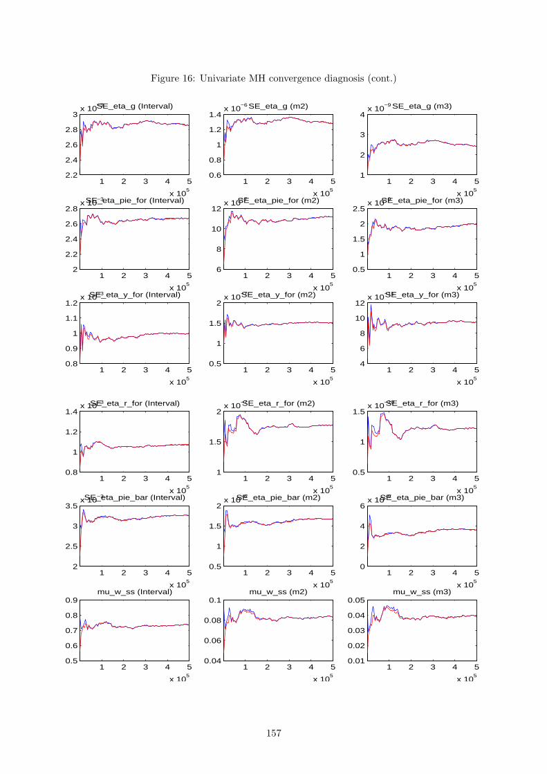
Figure 16: Univariate MH convergence diagnosis (cont.)
1 2 3 4 5
x 105
2.2
2.4
2.6
2.8
3x 10
−3SE_eta_g (Interval)
1 2 3 4 5
x 105
0.6
0.8
1
1.2
1.4x 10
−6 SE_eta_g (m2)
1 2 3 4 5
x 105
1
2
3
4x 10
−9 SE_eta_g (m3)
1 2 3 4 5
x 105
2
2.2
2.4
2.6
2.8x 10
−3SE_eta_pie_for (Interval)
1 2 3 4 5
x 105
6
8
10
12x 10
−7SE_eta_pie_for (m2)
1 2 3 4 5
x 105
0.5
1
1.5
2
2.5x 10
−9SE_eta_pie_for (m3)
1 2 3 4 5
x 105
0.8
0.9
1
1.1
1.2x 10
−3SE_eta_y_for (Interval)
1 2 3 4 5
x 105
0.5
1
1.5
2x 10
−7SE_eta_y_for (m2)
1 2 3 4 5
x 105
4
6
8
10
12x 10
−11SE_eta_y_for (m3)
1 2 3 4 5
x 105
0.8
1
1.2
1.4x 10
−3SE_eta_r_for (Interval)
1 2 3 4 5
x 105
1
1.5
2x 10
−7SE_eta_r_for (m2)
1 2 3 4 5
x 105
0.5
1
1.5x 10
−10SE_eta_r_for (m3)
1 2 3 4 5
x 105
2
2.5
3
3.5x 10
−3SE_eta_pie_bar (Interval)
1 2 3 4 5
x 105
0.5
1
1.5
2x 10
−6SE_eta_pie_bar (m2)
1 2 3 4 5
x 105
0
2
4
6x 10
−9SE_eta_pie_bar (m3)
1 2 3 4 5
x 105
0.5
0.6
0.7
0.8
0.9mu_w_ss (Interval)
1 2 3 4 5
x 105
0.04
0.06
0.08
0.1mu_w_ss (m2)
1 2 3 4 5
x 105
0.01
0.02
0.03
0.04
0.05mu_w_ss (m3)
157

Figure 17: Univariate MH convergence diagnosis (cont.)
1 2 3 4 5
x 105
0.7
0.8
0.9
1mu_d_ss (Interval)
1 2 3 4 5
x 105
0.05
0.1
0.15
0.2
0.25mu_d_ss (m2)
1 2 3 4 5
x 105
0
0.05
0.1
0.15
0.2mu_d_ss (m3)
1 2 3 4 5
x 105
0.4
0.5
0.6
0.7mu_m_ss (Interval)
1 2 3 4 5
x 105
0.02
0.04
0.06
0.08mu_m_ss (m2)
1 2 3 4 5
x 105
0
0.01
0.02
0.03
0.04mu_m_ss (m3)
1 2 3 4 5
x 105
0.5
0.6
0.7
0.8
0.9mu_c_ss (Interval)
1 2 3 4 5
x 105
0.05
0.1
0.15
0.2mu_c_ss (m2)
1 2 3 4 5
x 105
0.02
0.04
0.06
0.08
0.1mu_c_ss (m3)
1 2 3 4 5
x 105
0.2
0.3
0.4
0.5mu_i_ss (Interval)
1 2 3 4 5
x 105
0
0.02
0.04
0.06mu_i_ss (m2)
1 2 3 4 5
x 105
0
0.01
0.02
0.03mu_i_ss (m3)
1 2 3 4 5
x 105
0.2
0.3
0.4
0.5mu_g_ss (Interval)
1 2 3 4 5
x 105
0.01
0.02
0.03
0.04mu_g_ss (m2)
1 2 3 4 5
x 105
0
0.005
0.01
0.015mu_g_ss (m3)
1 2 3 4 5
x 105
0.35
0.4
0.45
0.5mu_x_ss (Interval)
1 2 3 4 5
x 105
0.02
0.025
0.03
0.035
0.04mu_x_ss (m2)
1 2 3 4 5
x 105
0.005
0.01
0.015mu_x_ss (m3)
158
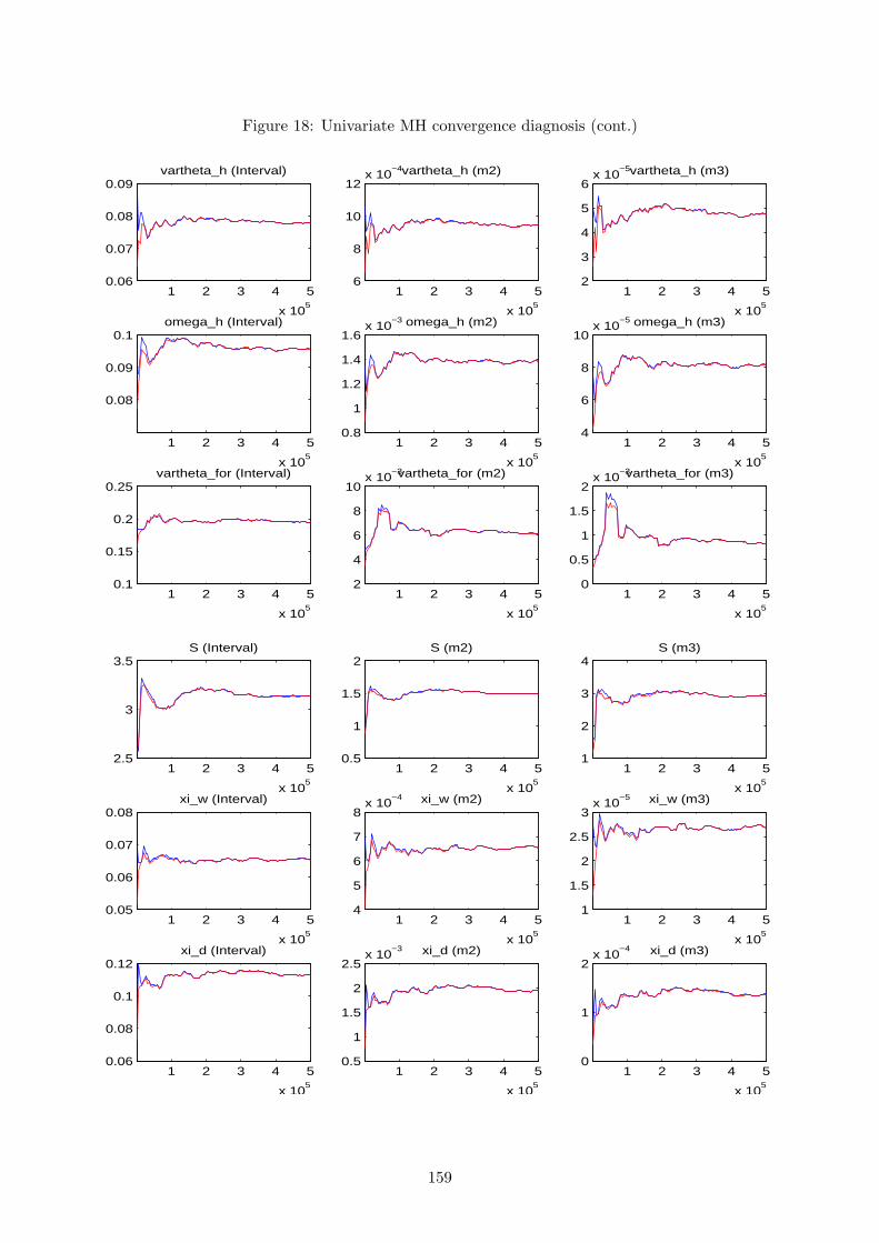
Figure 18: Univariate MH convergence diagnosis (cont.)
1 2 3 4 5
x 105
0.06
0.07
0.08
0.09vartheta_h (Interval)
1 2 3 4 5
x 105
6
8
10
12x 10
−4vartheta_h (m2)
1 2 3 4 5
x 105
2
3
4
5
6x 10
−5vartheta_h (m3)
1 2 3 4 5
x 105
0.08
0.09
0.1omega_h (Interval)
1 2 3 4 5
x 105
0.8
1
1.2
1.4
1.6x 10
−3 omega_h (m2)
1 2 3 4 5
x 105
4
6
8
10x 10
−5 omega_h (m3)
1 2 3 4 5
x 105
0.1
0.15
0.2
0.25vartheta_for (Interval)
1 2 3 4 5
x 105
2
4
6
8
10x 10
−3vartheta_for (m2)
1 2 3 4 5
x 105
0
0.5
1
1.5
2x 10
−3vartheta_for (m3)
1 2 3 4 5
x 105
2.5
3
3.5S (Interval)
1 2 3 4 5
x 105
0.5
1
1.5
2S (m2)
1 2 3 4 5
x 105
1
2
3
4S (m3)
1 2 3 4 5
x 105
0.05
0.06
0.07
0.08xi_w (Interval)
1 2 3 4 5
x 105
4
5
6
7
8x 10
−4 xi_w (m2)
1 2 3 4 5
x 105
1
1.5
2
2.5
3x 10
−5 xi_w (m3)
1 2 3 4 5
x 105
0.06
0.08
0.1
0.12xi_d (Interval)
1 2 3 4 5
x 105
0.5
1
1.5
2
2.5x 10
−3 xi_d (m2)
1 2 3 4 5
x 105
0
1
2x 10
−4 xi_d (m3)
159
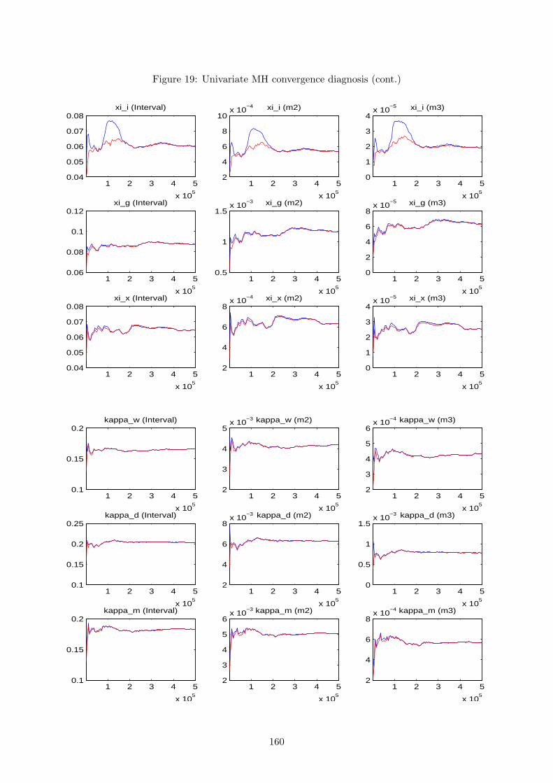
Figure 19: Univariate MH convergence diagnosis (cont.)
1 2 3 4 5
x 105
0.04
0.05
0.06
0.07
0.08xi_i (Interval)
1 2 3 4 5
x 105
2
4
6
8
10x 10
−4 xi_i (m2)
1 2 3 4 5
x 105
0
1
2
3
4x 10
−5 xi_i (m3)
1 2 3 4 5
x 105
0.06
0.08
0.1
0.12xi_g (Interval)
1 2 3 4 5
x 105
0.5
1
1.5x 10
−3 xi_g (m2)
1 2 3 4 5
x 105
0
2
4
6
8x 10
−5 xi_g (m3)
1 2 3 4 5
x 105
0.04
0.05
0.06
0.07
0.08xi_x (Interval)
1 2 3 4 5
x 105
2
4
6
8x 10
−4 xi_x (m2)
1 2 3 4 5
x 105
0
1
2
3
4x 10
−5 xi_x (m3)
1 2 3 4 5
x 105
0.1
0.15
0.2kappa_w (Interval)
1 2 3 4 5
x 105
2
3
4
5x 10
−3 kappa_w (m2)
1 2 3 4 5
x 105
2
3
4
5
6x 10
−4 kappa_w (m3)
1 2 3 4 5
x 105
0.1
0.15
0.2
0.25kappa_d (Interval)
1 2 3 4 5
x 105
2
4
6
8x 10
−3 kappa_d (m2)
1 2 3 4 5
x 105
0
0.5
1
1.5x 10
−3 kappa_d (m3)
1 2 3 4 5
x 105
0.1
0.15
0.2kappa_m (Interval)
1 2 3 4 5
x 105
2
3
4
5
6x 10
−3 kappa_m (m2)
1 2 3 4 5
x 105
2
4
6
8x 10
−4 kappa_m (m3)
160

Figure 20: Univariate MH convergence diagnosis (cont.)
1 2 3 4 5
x 105
0.16
0.18
0.2
0.22
0.24kappa_c (Interval)
1 2 3 4 5
x 105
4
6
8
10x 10
−3 kappa_c (m2)
1 2 3 4 5
x 105
0
0.5
1
1.5x 10
−3 kappa_c (m3)
1 2 3 4 5
x 105
0.2
0.25
0.3
0.35kappa_i (Interval)
1 2 3 4 5
x 105
4
6
8
10x 10
−3 kappa_i (m2)
1 2 3 4 5
x 105
0
0.5
1
1.5x 10
−3 kappa_i (m3)
1 2 3 4 5
x 105
0.2
0.22
0.24
0.26kappa_g (Interval)
1 2 3 4 5
x 105
6
7
8
9
10x 10
−3 kappa_g (m2)
1 2 3 4 5
x 105
0.8
1
1.2
1.4
1.6x 10
−3 kappa_g (m3)
1 2 3 4 5
x 105
0.16
0.18
0.2
0.22
0.24kappa_x (Interval)
1 2 3 4 5
x 105
4
6
8
10x 10
−3 kappa_x (m2)
1 2 3 4 5
x 105
0
0.5
1
1.5x 10
−3 kappa_x (m3)
1 2 3 4 5
x 105
0.2
0.25
0.3rho_eps_i (Interval)
1 2 3 4 5
x 105
4
6
8
10x 10
−3 rho_eps_i (m2)
1 2 3 4 5
x 105
0.5
1
1.5x 10
−3 rho_eps_i (m3)
1 2 3 4 5
x 105
0.22
0.24
0.26
0.28
0.3rho_eps_c (Interval)
1 2 3 4 5
x 105
6
8
10
12x 10
−3rho_eps_c (m2)
1 2 3 4 5
x 105
1
1.2
1.4
1.6
1.8x 10
−3rho_eps_c (m3)
161
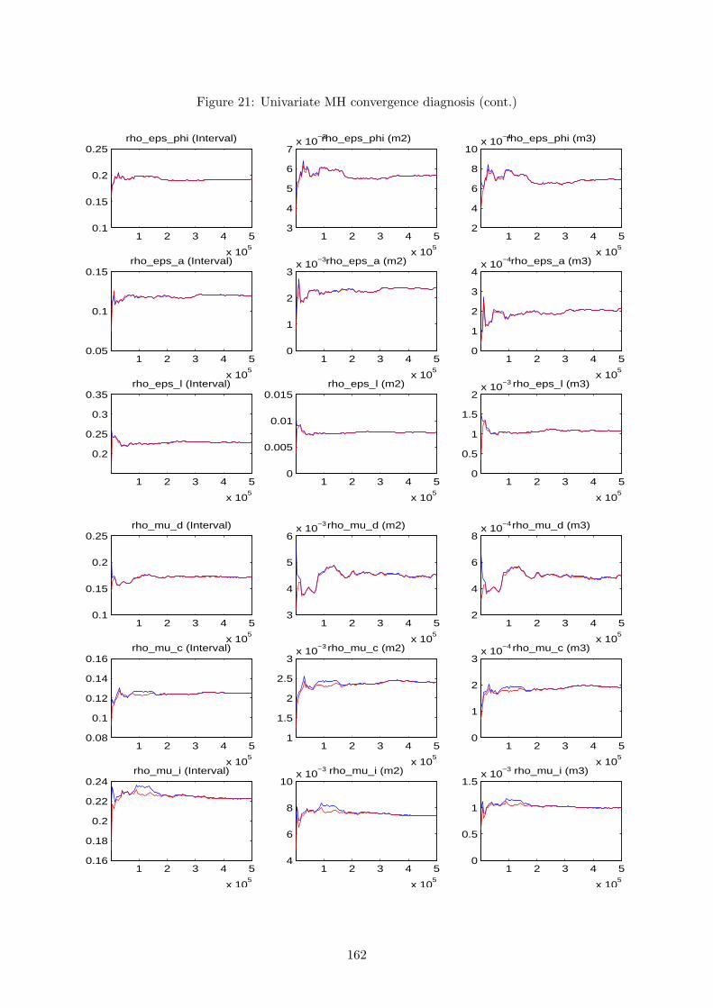
Figure 21: Univariate MH convergence diagnosis (cont.)
1 2 3 4 5
x 105
0.1
0.15
0.2
0.25rho_eps_phi (Interval)
1 2 3 4 5
x 105
3
4
5
6
7x 10
−3rho_eps_phi (m2)
1 2 3 4 5
x 105
2
4
6
8
10x 10
−4rho_eps_phi (m3)
1 2 3 4 5
x 105
0.05
0.1
0.15rho_eps_a (Interval)
1 2 3 4 5
x 105
0
1
2
3x 10
−3rho_eps_a (m2)
1 2 3 4 5
x 105
0
1
2
3
4x 10
−4rho_eps_a (m3)
1 2 3 4 5
x 105
0.2
0.25
0.3
0.35rho_eps_l (Interval)
1 2 3 4 5
x 105
0
0.005
0.01
0.015rho_eps_l (m2)
1 2 3 4 5
x 105
0
0.5
1
1.5
2x 10
−3 rho_eps_l (m3)
1 2 3 4 5
x 105
0.1
0.15
0.2
0.25rho_mu_d (Interval)
1 2 3 4 5
x 105
3
4
5
6x 10
−3rho_mu_d (m2)
1 2 3 4 5
x 105
2
4
6
8x 10
−4rho_mu_d (m3)
1 2 3 4 5
x 105
0.08
0.1
0.12
0.14
0.16rho_mu_c (Interval)
1 2 3 4 5
x 105
1
1.5
2
2.5
3x 10
−3 rho_mu_c (m2)
1 2 3 4 5
x 105
0
1
2
3x 10
−4 rho_mu_c (m3)
1 2 3 4 5
x 105
0.16
0.18
0.2
0.22
0.24rho_mu_i (Interval)
1 2 3 4 5
x 105
4
6
8
10x 10
−3 rho_mu_i (m2)
1 2 3 4 5
x 105
0
0.5
1
1.5x 10
−3 rho_mu_i (m3)
162
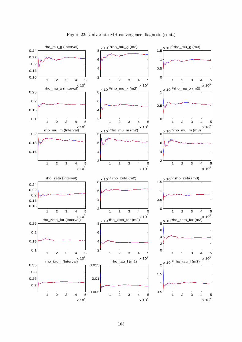
Figure 22: Univariate MH convergence diagnosis (cont.)
1 2 3 4 5
x 105
0.16
0.18
0.2
0.22
0.24rho_mu_g (Interval)
1 2 3 4 5
x 105
2
4
6
8x 10
−3rho_mu_g (m2)
1 2 3 4 5
x 105
0
0.5
1
1.5x 10
−3rho_mu_g (m3)
1 2 3 4 5
x 105
0.1
0.15
0.2
0.25rho_mu_x (Interval)
1 2 3 4 5
x 105
2
4
6
8x 10
−3 rho_mu_x (m2)
1 2 3 4 5
x 105
0
0.5
1x 10
−3 rho_mu_x (m3)
1 2 3 4 5
x 105
0.16
0.18
0.2rho_mu_m (Interval)
1 2 3 4 5
x 105
3
4
5
6x 10
−3rho_mu_m (m2)
1 2 3 4 5
x 105
2
4
6
8x 10
−4rho_mu_m (m3)
1 2 3 4 5
x 105
0.16
0.18
0.2
0.22
0.24
rho_zeta (Interval)
1 2 3 4 5
x 105
2
4
6
8x 10
−3 rho_zeta (m2)
1 2 3 4 5
x 105
0
0.5
1
1.5x 10
−3 rho_zeta (m3)
1 2 3 4 5
x 105
0.1
0.15
0.2
0.25rho_zeta_for (Interval)
1 2 3 4 5
x 105
2
4
6
8x 10
−3rho_zeta_for (m2)
1 2 3 4 5
x 105
0
2
4
6
8x 10
−4rho_zeta_for (m3)
1 2 3 4 5
x 105
0.2
0.25
0.3
0.35rho_tau_l (Interval)
1 2 3 4 5
x 105
0.005
0.01
0.015rho_tau_l (m2)
1 2 3 4 5
x 105
0.5
1
1.5
2x 10
−3 rho_tau_l (m3)
163
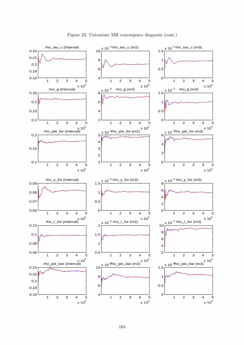
Figure 23: Univariate MH convergence diagnosis (cont.)
1 2 3 4 5
x 105
0.16
0.18
0.2
0.22
0.24rho_tau_c (Interval)
1 2 3 4 5
x 105
4
6
8
10x 10
−3 rho_tau_c (m2)
1 2 3 4 5
x 105
0
0.5
1
1.5x 10
−3 rho_tau_c (m3)
1 2 3 4 5
x 105
0.1
0.15
0.2
0.25rho_g (Interval)
1 2 3 4 5
x 105
2
4
6
8x 10
−3 rho_g (m2)
1 2 3 4 5
x 105
0
0.5
1
1.5x 10
−3 rho_g (m3)
1 2 3 4 5
x 105
0.1
0.15
0.2rho_pie_for (Interval)
1 2 3 4 5
x 105
1
2
3
4
5x 10
−3rho_pie_for (m2)
1 2 3 4 5
x 105
0
2
4
6x 10
−4rho_pie_for (m3)
1 2 3 4 5
x 105
0.06
0.07
0.08
0.09rho_y_for (Interval)
1 2 3 4 5
x 105
0
0.5
1
1.5x 10
−3 rho_y_for (m2)
1 2 3 4 5
x 105
0
2
4
6
8x 10
−5 rho_y_for (m3)
1 2 3 4 5
x 105
0.06
0.08
0.1
0.12rho_r_for (Interval)
1 2 3 4 5
x 105
0.5
1
1.5
2x 10
−3 rho_r_for (m2)
1 2 3 4 5
x 105
2
4
6
8
10x 10
−5 rho_r_for (m3)
1 2 3 4 5
x 105
0.16
0.18
0.2
0.22
0.24rho_pie_bar (Interval)
1 2 3 4 5
x 105
4
6
8
10x 10
−3rho_pie_bar (m2)
1 2 3 4 5
x 105
0
0.5
1
1.5x 10
−3rho_pie_bar (m3)
164