Bayesian Deep Learning | Uncertainty in Deep...
33
Chapter 3 Bayesian Deep Learning In previous chapters we reviewed Bayesian neural networks (BNNs) and historical tech- niques for approximate inference in these, as well as more recent approaches. We discussed the advantages and disadvantages of different techniques, examining their practicality. This, perhaps, is the most important aspect of modern techniques for approximate infer- ence in BNNs. The field of deep learning is pushed forward by practitioners, working on real-world problems. Techniques which cannot scale to complex models with potentially millions of parameters, scale well with large amounts of data, need well studied models to be radically changed, or are not accessible to engineers, will simply perish. In this chapter we will develop on the strand of work of [Graves, 2011; Hinton and Van Camp, 1993], but will do so from the Bayesian perspective rather than the information theory one. Developing Bayesian approaches to deep learning, we will tie approximate BNN inference together with deep learning stochastic regularisation techniques (SRTs) such as dropout. These regularisation techniques are used in many modern deep learning tools, allowing us to offer a practical inference technique. We will start by reviewing in detail the tools used by Graves [2011], and extend on these with recent research. In the process we will comment and analyse the variance of several stochastic estimators used in variational inference (VI). Following that we will tie these derivations to SRTs, and propose practical techniques to obtain model uncertainty, even from existing models. We finish the chapter by developing specific examples for image based models (CNNs) and sequence based models (RNNs). These will be demonstrated in chapter 5, where we will survey recent research making use of the suggested tools in real-world problems.
Transcript of Bayesian Deep Learning | Uncertainty in Deep...
Chapter 3
Bayesian Deep Learning
In previous chapters we reviewed Bayesian neural networks (BNNs) and historical tech-
niques for approximate inference in these, as well as more recent approaches. We discussed
the advantages and disadvantages of different techniques, examining their practicality.
This, perhaps, is the most important aspect of modern techniques for approximate infer-
ence in BNNs. The field of deep learning is pushed forward by practitioners, working on
real-world problems. Techniques which cannot scale to complex models with potentially
millions of parameters, scale well with large amounts of data, need well studied models
to be radically changed, or are not accessible to engineers, will simply perish.
In this chapter we will develop on the strand of work of [Graves, 2011; Hinton and
Van Camp, 1993], but will do so from the Bayesian perspective rather than the information
theory one. Developing Bayesian approaches to deep learning, we will tie approximate
BNN inference together with deep learning stochastic regularisation techniques (SRTs)
such as dropout. These regularisation techniques are used in many modern deep learning
tools, allowing us to offer a practical inference technique.
We will start by reviewing in detail the tools used by Graves [2011], and extend on
these with recent research. In the process we will comment and analyse the variance
of several stochastic estimators used in variational inference (VI). Following that we
will tie these derivations to SRTs, and propose practical techniques to obtain model
uncertainty, even from existing models. We finish the chapter by developing specific
examples for image based models (CNNs) and sequence based models (RNNs). These
will be demonstrated in chapter 5, where we will survey recent research making use of
the suggested tools in real-world problems.

30 Bayesian Deep Learning
3.1 Advanced techniques in variational inference
We start by reviewing recent advances in VI. We are interested in the posterior over the
weights given our observables X, Y: p(ω♣X, Y
. This posterior is not tractable for a
Bayesian NN, and we use variational inference to approximate it. Recall our minimisation
objective (eq. (2.6)),
LVI(θ) := −N∑
i=1
∫qθ(ω) log p(yi♣f
ω(xi))dω + KL(qθ(ω)♣♣p(ω)). (3.1)
Evaluating this objective poses several difficulties. First, the summed-over terms∫
qθ(ω) log p(yi♣fω(xi))dω are not tractable for BNNs with more than a single hidden
layer. Second, this objective requires us to perform computations over the entire dataset,
which can be too costly for large N .
To solve the latter problem, we may use data sub-sampling (also referred to as
mini-batch optimisation). We approximate eq. (3.1) with
LVI(θ) := −N
M
∑
i∈S
∫qθ(ω) log p(yi♣f
ω(xi))dω + KL(qθ(ω)♣♣p(ω)) (3.2)
with a random index set S of size M .
The data sub-sampling approximation forms an unbiased stochastic estimator to eq.
(3.1), meaning that ES[LVI(θ)] = LVI(θ). We can thus use a stochastic optimiser to
optimise this stochastic objective, and obtain a (local) optimum θ∗ which would be an
optimum to LVI(θ) as well [Robbins and Monro, 1951]. This approximation is often used
in the deep learning literature, and was suggested by Hoffman et al. [2013] in the VI
context (surprisingly) only recently1.
The remaining difficulty with the objective in eq. (3.1) is the evaluation of the expected
log likelihood∫
qθ(ω) log p(yi♣fω(xi))dω. Monte Carlo integration of the integral has
been attempted by some, to varying degrees of success. We will review three approaches
used in the VI literature and analyse their variance.
3.1.1 Monte Carlo estimators in variational inference
We often use Monte Carlo (MC) estimation in variational inference to estimate the
expected log likelihood (the integral in eq. (3.2)). But more importantly we wish to
estimate the expected log likelihood’s derivatives w.r.t. the approximating distribution
1Although online VI methods processing one point at a time have a long history [Ghahramani andAttias, 2000; Sato, 2001]
3.1 Advanced techniques in variational inference 31
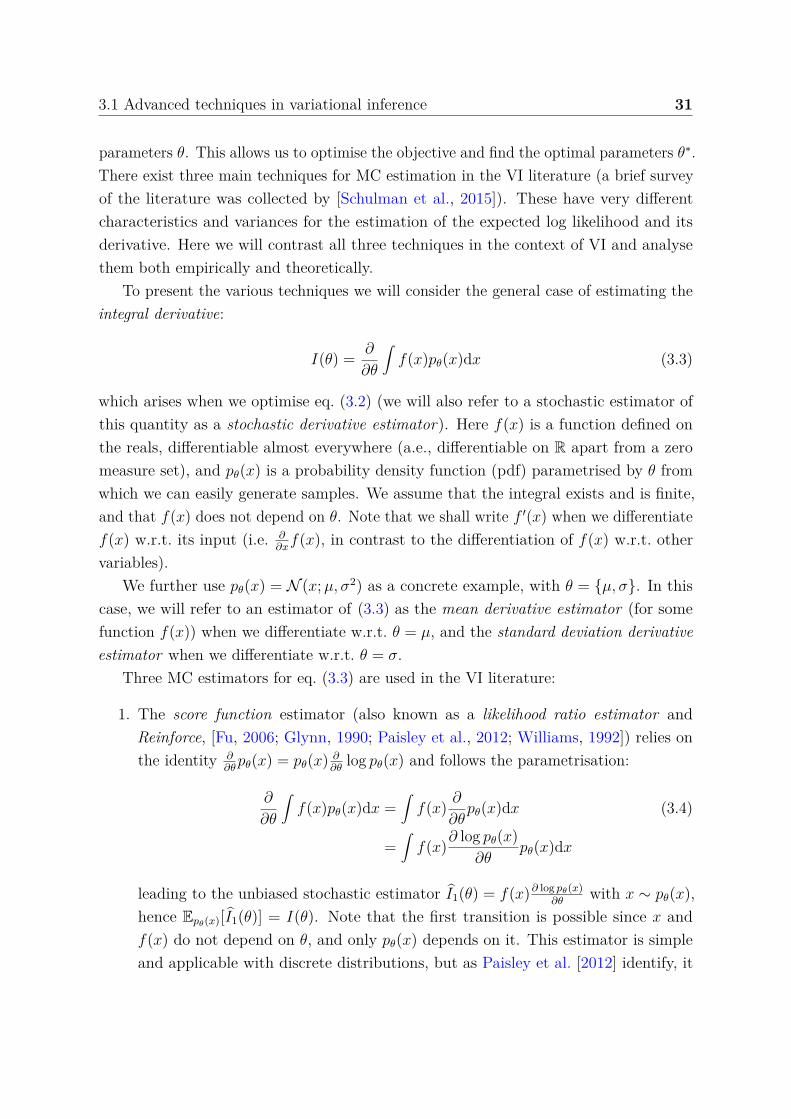
parameters θ. This allows us to optimise the objective and find the optimal parameters θ∗.
There exist three main techniques for MC estimation in the VI literature (a brief survey
of the literature was collected by [Schulman et al., 2015]). These have very different
characteristics and variances for the estimation of the expected log likelihood and its
derivative. Here we will contrast all three techniques in the context of VI and analyse
them both empirically and theoretically.
To present the various techniques we will consider the general case of estimating the
integral derivative:
I(θ) =∂
∂θ
∫f(x)pθ(x)dx (3.3)
which arises when we optimise eq. (3.2) (we will also refer to a stochastic estimator of
this quantity as a stochastic derivative estimator). Here f(x) is a function defined on
the reals, differentiable almost everywhere (a.e., differentiable on R apart from a zero
measure set), and pθ(x) is a probability density function (pdf) parametrised by θ from
which we can easily generate samples. We assume that the integral exists and is finite,
and that f(x) does not depend on θ. Note that we shall write f ′(x) when we differentiate
f(x) w.r.t. its input (i.e. ∂∂x
f(x), in contrast to the differentiation of f(x) w.r.t. other
variables).
We further use pθ(x) = N (x; µ, σ2) as a concrete example, with θ = ¶µ, σ♢. In this
case, we will refer to an estimator of (3.3) as the mean derivative estimator (for some
function f(x)) when we differentiate w.r.t. θ = µ, and the standard deviation derivative
estimator when we differentiate w.r.t. θ = σ.
Three MC estimators for eq. (3.3) are used in the VI literature:
1. The score function estimator (also known as a likelihood ratio estimator and
Reinforce, [Fu, 2006; Glynn, 1990; Paisley et al., 2012; Williams, 1992]) relies on
the identity ∂∂θ
pθ(x) = pθ(x) ∂∂θ
log pθ(x) and follows the parametrisation:
∂
∂θ
∫f(x)pθ(x)dx =
∫f(x)
∂
∂θpθ(x)dx (3.4)
=∫
f(x)∂ log pθ(x)
∂θpθ(x)dx
leading to the unbiased stochastic estimator I1(θ) = f(x)∂ log pθ(x)∂θ
with x ∼ pθ(x),
hence Epθ(x)[I1(θ)] = I(θ). Note that the first transition is possible since x and
f(x) do not depend on θ, and only pθ(x) depends on it. This estimator is simple
and applicable with discrete distributions, but as Paisley et al. [2012] identify, it

32 Bayesian Deep Learning
has rather high variance. When used in practice it is often coupled with a variance
reduction technique.
2. Eq. (3.3) can be re-parametrised to obtain an alternative MC estimator, which we
refer to as a pathwise derivative estimator (this estimator is also referred to in the
literature as the re-parametrisation trick, infinitesimal perturbation analysis, and
stochastic backpropagation [Glasserman, 2013; Kingma and Welling, 2013, 2014;
Rezende et al., 2014; Titsias and Lázaro-Gredilla, 2014]). Assume that pθ(x) can
be re-parametrised as p(ϵ), a parameter-free distribution, s.t. x = g(θ, ϵ) with a
deterministic differentiable bivariate transformation g(·, ·). For example, with our
pθ(x) = N (x; µ, σ2) we have g(θ, ϵ) = µ + σϵ together with p(ϵ) = N (ϵ; 0, I). Then
the following estimator arises:
I2(θ) = f ′(g(θ, ϵ))∂
∂θg(θ, ϵ). (3.5)
Here Ep(ϵ)[I2(θ)] = I(θ).
Note that compared to the estimator above where f(x) is used, in this case we use
its derivative f ′(x). In the Gaussian case, both the derivative w.r.t. µ as well as
the derivative w.r.t. σ use f(x)’s first derivative (note the substitution of ϵ with
x = µ + σϵ):
∂
∂µ
∫f(x)pθ(x)dx =
∫f ′(x)pθ(x)dx,
∂
∂σ
∫f(x)pθ(x)dx =
∫f ′(x)
(x− µ)
σpθ(x)dx,
i.e. I2(µ) = f ′(x) and I2(σ) = f ′(x) (x−µ)σ
with Epθ(x)[I2(µ)] = I(µ) and Epθ(x)[I2(σ)] =
I(σ). An interesting question arises when we compare this estimator (I2(θ)) to
the one above (I1(θ)): why is it that in one case we use the function f(x), and in
the other use its derivative? This is answered below, together with an alternative
derivation to that of Kingma and Welling [2013, section 2.4].
The pathwise derivative estimator seems to (empirically) result in a lower variance
estimator than the one above, although to the best of my knowledge no proof to this
has been given in the literature. An analysis of this parametrisation, together with
examples where the estimator has higher variance than that of the score function
estimator is given below.

3.1 Advanced techniques in variational inference 33
3. Lastly, it is important to mention the estimator given in [Opper and Archambeau,
2009, eq. (6-7)] (studied in [Rezende et al., 2014] as well). Compared to both
estimators above, Opper and Archambeau [2009] relied on the characteristic function
of the Gaussian distribution, restricting the estimator to Gaussian pθ(x) alone.
The resulting mean derivative estimator, ∂∂µ
∫f(x)pθ(x)dx, is identical to the one
resulting from the pathwise derivative estimator.
But when differentiating w.r.t. σ, the estimator depends on f(x)’s second derivative
[Opper and Archambeau, 2009, eq. (19)]:
∂
∂σ
∫f(x)pθ(x)dx = 2σ ·
1
2
∫f ′′(x)pθ(x)dx (3.6)
i.e. I3(σ) = σf ′′(x) with Epθ(x)[I3(σ)] = I(σ). This is in comparison to the
estimators above that use f(x) or its first derivative. We refer to this estimator as
a characteristic function estimator.
These three MC estimators are believed to have decreasing estimator variances (1) >
(2) > (3). Before we analyse this variance, we offer an alternative derivation to Kingma
and Welling [2013]’s derivation of the pathwise derivative estimator.
Remark (Auxiliary variable view of the pathwise derivative estimator). Kingma
and Welling [2013]’s derivation of the pathwise derivative estimator was obtained
through a change of variables. Instead we justify the estimator through a construc-
tion relying on an auxiliary variable augmenting the distribution pθ(x).
Assume that the distribution pθ(x) can be written as∫
pθ(x, ϵ)dϵ =∫
pθ(x♣ϵ)p(ϵ)dϵ,
with pθ(x♣ϵ) = δ(x− g(θ, ϵ)) a dirac delta function. Then
∂
∂θ
∫f(x)pθ(x)dx =
∂
∂θ
∫f(x)
(∫pθ(x, ϵ)dϵ
)dx
=∂
∂θ
∫f(x)pθ(x♣ϵ)p(ϵ)dϵdx
=∂
∂θ
∫ ( ∫f(x)δ
(x− g(θ, ϵ)
dx
)p(ϵ)dϵ.
Now, since δ(x− g(θ, ϵ)) is zero for all x apart from x = g(θ, ϵ),
∂
∂θ
∫ ( ∫f(x)δ
(x− g(θ, ϵ)
dx
)p(ϵ)dϵ =
∂
∂θ
∫f(g(θ, ϵ))p(ϵ)dϵ
34 Bayesian Deep Learning
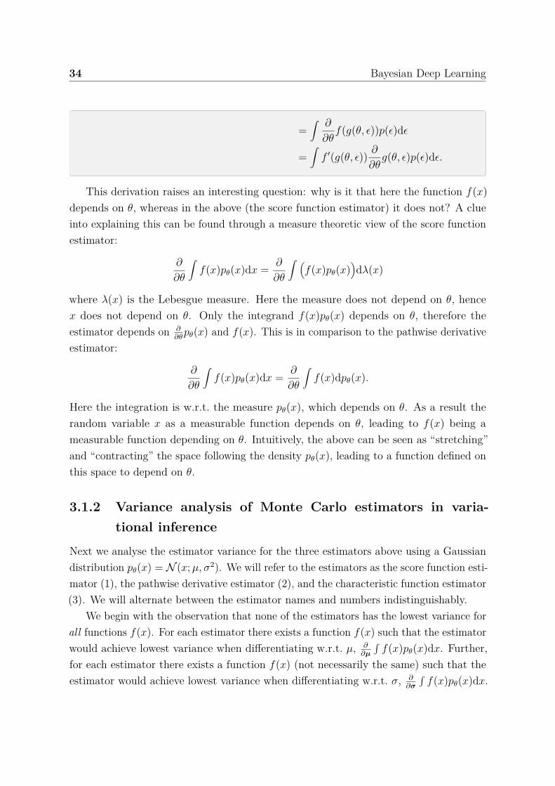
=∫ ∂
∂θf(g(θ, ϵ))p(ϵ)dϵ
=∫
f ′(g(θ, ϵ))∂
∂θg(θ, ϵ)p(ϵ)dϵ.
This derivation raises an interesting question: why is it that here the function f(x)
depends on θ, whereas in the above (the score function estimator) it does not? A clue
into explaining this can be found through a measure theoretic view of the score function
estimator:
∂
∂θ
∫f(x)pθ(x)dx =
∂
∂θ
∫ (f(x)pθ(x)
dλ(x)
where λ(x) is the Lebesgue measure. Here the measure does not depend on θ, hence
x does not depend on θ. Only the integrand f(x)pθ(x) depends on θ, therefore the
estimator depends on ∂∂θ
pθ(x) and f(x). This is in comparison to the pathwise derivative
estimator:
∂
∂θ
∫f(x)pθ(x)dx =
∂
∂θ
∫f(x)dpθ(x).
Here the integration is w.r.t. the measure pθ(x), which depends on θ. As a result the
random variable x as a measurable function depends on θ, leading to f(x) being a
measurable function depending on θ. Intuitively, the above can be seen as “stretching”
and “contracting” the space following the density pθ(x), leading to a function defined on
this space to depend on θ.
3.1.2 Variance analysis of Monte Carlo estimators in varia-
tional inference
Next we analyse the estimator variance for the three estimators above using a Gaussian
distribution pθ(x) = N (x; µ, σ2). We will refer to the estimators as the score function esti-
mator (1), the pathwise derivative estimator (2), and the characteristic function estimator
(3). We will alternate between the estimator names and numbers indistinguishably.
We begin with the observation that none of the estimators has the lowest variance for
all functions f(x). For each estimator there exists a function f(x) such that the estimator
would achieve lowest variance when differentiating w.r.t. µ, ∂∂µ
∫f(x)pθ(x)dx. Further,
for each estimator there exists a function f(x) (not necessarily the same) such that the
estimator would achieve lowest variance when differentiating w.r.t. σ, ∂∂σ
∫f(x)pθ(x)dx.

3.1 Advanced techniques in variational inference 35
f(x) Score Pathwise Character.function derivative function
x + x2 1.7 · 1014.0 · 10
04.0 · 10
0
sin(x) 3.3 · 10−12.0 · 10
−12.0 · 10
−1
sin(10x) 5.0 · 10−1 5.0 · 101 5.0 · 101
Table 3.1 ∂∂µ
∫f(x)pθ(x)dx variance
f(x) Score Pathwise Character.function derivative function
x + x2 8.6 · 101 9.1 · 1000.0 · 10
0
sin(x) 8.7 · 10−13.0 · 10
−1 4.3 · 10−1
sin(10x) 1.0 · 100 5.0 · 101 5.0 · 103
Table 3.2 ∂∂σ
∫f(x)pθ(x)dx variance
Table 3.3 Estimator variance for various functions f(x) for the score function estimator,the pathwise derivative estimator, and the characteristic function estimator ((1), (2),and (3) above). On the left is mean derivative estimator variance, and on the right isstandard deviation derivative estimator variance, both w.r.t. pθ = N (µ, σ2) and evaluatedat µ = 0, σ = 1. In bold is lowest estimator variance.
We assess empirical sample variance of T = 106 samples for the mean and standard
deviation derivative estimators. Tables 3.1 and 3.2 show estimator sample variance for
the integral derivative w.r.t. µ and σ respectively, for three different functions f(x). Even
though all estimators result in roughly the same means, their variances differ considerably.
For functions with slowly varying derivatives in a neighbourhood of zero (such as the
smooth function f(x) = x + x2) we have that the estimator variance obeys (1) > (2) >
(3). Also note that mean variance for (2) and (3) are identical, and that σ derivative
variance under the characteristic function estimator in this case is zero (since the second
derivative for this function is zero). Lastly, note that even though f(x) = sin(x) is
smooth with bounded derivatives, the similar function f(x) = sin(10x) has variance (3)
> (2) > (1). This is because the derivative of the function has high magnitude and varies
much near zero.
I will provide a simple property a function has to satisfy for it to have lower variance
under the pathwise derivative estimator and the characteristic function estimator than
the score function estimator. This will be for the mean derivative estimator.
Proposition 1. Let f(x), f ′(x), f ′′(x) be real-valued functions s.t. f(x) is an indefinite
integral of f ′(x), and f ′(x) is an indefinite integral of f ′′(x). Assume that Varpθ(x)((x−
µ)f(x)) <∞, and Varpθ(x)(f′(x)) <∞, as well as Epθ(x)(♣(x−µ)f ′(x) + f(x)♣) <∞ and
Epθ(x)(♣f′′(x)♣) <∞, with pθ(x) = N (µ, σ2).
If it holds that
Epθ(x)
((x− µ)f ′(x) + f(x)
2− σ4
Epθ(x)
(f ′′(x)2
≥ 0,
then the pathwise derivative and the characteristic function mean derivative estimators
w.r.t. the function f(x) will have lower variance than the score function estimator.

36 Bayesian Deep Learning
Before proving the proposition, I will give some intuitive insights into what the
condition means. For this, assume for simplicity that µ = 0 and σ = 1. This gives the
simplified condition
Epθ(x)
(xf ′(x) + f(x)
2≥ Epθ(x)
(f ′′(x)2
.
First, observe that all expectations are taken over pθ(x), meaning that we only care
about the functions’ average behaviour near zero. Second, a function f(x) with a large
derivative absolute value will change considerably, hence will have high variance. Since
the pathwise derivative estimator boils down to f ′(x) in the Gaussian case, and the score
function estimator boils down to xf(x) (shown in the proof), we wish the expected change
in ∂∂x
xf(x) = xf ′(x) + f(x) to be higher than the expected change in ∂∂x
f ′(x) = f ′′(x),
hence the condition.
Proof. We start with the observation that the score function mean estimator w.r.t. a
Gaussian pθ(x) is given by
∂
∂µ
∫f(x)pθ(x)dx =
∫f(x)
x− µ
σ2pθ(x)dx
resulting in the estimator I1 = f(x)x−µσ2 . The pathwise derivative and the characteristic
function estimators are identical for the mean derivative, and given by I2 = f ′(x). We
thus wish to show that Varpθ(x)(I2) ≤ Varpθ(x)(I1) under the proposition’s assumptions.
Since Varpθ(x)(I1) =Varpθ(x)(xf(x)−µf(x))
σ4 , we wish to show that
σ4Varpθ(x)
(f ′(x)
≤ Varpθ(x)
((x− µ)f(x)
.
Proposition 3.2 in [Cacoullos, 1982] states that for g(x), g′(x) real-valued functions s.t.
g(x) is an indefinite integral of g′(x), and Varpθ(x)(g(x)) < ∞ and Epθ(x)(♣g′(x)♣) < ∞,
there exists that
σ2Epθ(x)
(g′(x)
2≤ Varpθ(x)
(g(x)
≤ σ2
Epθ(x)
(g′(x)2
.
Substituting g(x) with (x− µ)f(x) we have
σ2Epθ(x)
((x− µ)f ′(x) + f(x)
2≤ Varpθ(x)
((x− µ)f(x)
3.2 Practical inference in Bayesian neural networks 37
and substituting g(x) with f ′(x) we have
Varpθ(x)
(f ′(x)
≤ σ2
Epθ(x)
(f ′′(x)2
.
Under the proposition’s assumption that
Epθ(x)
((x− µ)f ′(x) + f(x)
2− σ4
Epθ(x)
(f ′′(x)2
≥ 0
we conclude
σ4Varpθ(x)
(f ′(x)
≤ σ6
Epθ(x)
(f ′′(x)2
≤ σ2
Epθ(x)
((x− µ)f ′(x) + f(x)
2
≤ Varpθ(x)
((x− µ)f(x)
as we wanted to show.
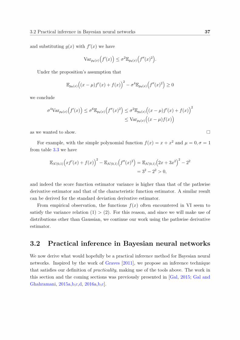
For example, with the simple polynomial function f(x) = x + x2 and µ = 0, σ = 1
from table 3.3 we have
EN (0,1)
(xf ′(x) + f(x)
2− EN (0,1)
(f ′′(x)2
= EN (0,1)
(2x + 3x2
2− 22
= 32 − 22 > 0,
and indeed the score function estimator variance is higher than that of the pathwise
derivative estimator and that of the characteristic function estimator. A similar result
can be derived for the standard deviation derivative estimator.
From empirical observation, the functions f(x) often encountered in VI seem to
satisfy the variance relation (1) > (2). For this reason, and since we will make use of
distributions other than Gaussian, we continue our work using the pathwise derivative
estimator.
3.2 Practical inference in Bayesian neural networks
We now derive what would hopefully be a practical inference method for Bayesian neural
networks. Inspired by the work of Graves [2011], we propose an inference technique
that satisfies our definition of practicality, making use of the tools above. The work in
this section and the coming sections was previously presented in [Gal, 2015; Gal and
Ghahramani, 2015a,b,c,d, 2016a,b,c].

38 Bayesian Deep Learning
In his work, Graves [2011] used both delta approximating distributions, as well as fully
factorised Gaussian approximating distributions. As such, Graves [2011] relied on Opper
and Archambeau [2009]’s characteristic function estimator in his approximation of eq.
(3.2). Further, Graves [2011] factorised the approximating distribution for each weight
scalar, losing weight correlations. This approach has led to the limitations discussed in
§2.2.2, hurting the method’s performance and practicality.
Using the tools above, and relying on the pathwise derivative estimator instead of
the characteristic function estimator in particular, we can make use of more interesting
non-Gaussian approximating distributions. Further, to avoid losing weight correlations,
we factorise the distribution for each weight row wl,i in each weight matrix Wl, instead
of factorising over each weight scalar. The reason for this will be given below. Using
these two key changes, we will see below how our approximate inference can be closely
tied to SRTs, suggesting a practical, well performing, implementation.
To use the pathwise derivative estimator we need to re-parametrise each qθl,i(wl,i) as
wl,i = g(θl,i, ϵl,i) and specify some p(ϵl,i) (this will be done at a later time). For simplicity
of notation we will write p(ϵ) =∏
l,i p(ϵl,i), and ω = g(θ, ϵ) collecting all model random
variables. Starting from the data sub-sampling objective (eq. (3.2)), we re-parametrise
each integral to integrate w.r.t. p(ϵ):
LVI(θ) = −N
M
∑
i∈S
∫qθ(ω) log p(yi♣f
ω(xi))dω + KL(qθ(ω)♣♣p(ω))
= −N
M
∑
i∈S
∫p(ϵ) log p(yi♣f
g(θ,ϵ)(xi))dϵ + KL(qθ(ω)♣♣p(ω))
and then replace each expected log likelihood term with its stochastic estimator (eq.
(3.5)), resulting in a new MC estimator:
LMC(θ) = −N
M
∑
i∈S
log p(yi♣fg(θ,ϵ)(xi)) + KL(qθ(ω)♣♣p(ω)) (3.7)
s.t. ES,ϵ(LMC(θ)) = LVI(θ).
Following results in stochastic non-convex optimisation [Rubin, 1981], optimising
LMC(θ) w.r.t. θ would converge to the same optima as optimising our original objective
LVI(θ). One thus follows algorithm 1 for inference.
Predictions with this approximation follow equation (2.4) which replaces the posterior
p(ω♣X, Y) with the approximate posterior qθ(ω). We can then approximate the predictive

3.2 Practical inference in Bayesian neural networks 39
Algorithm 1 Minimise divergence between qθ(ω) and p(ω♣X, Y )
1: Given dataset X, Y,2: Define learning rate schedule η,3: Initialise parameters θ randomly.4: repeat
5: Sample M random variables ϵi ∼ p(ϵ), S a random subset of ¶1, .., N♢ of size M .6: Calculate stochastic derivative estimator w.r.t. θ:
∆θ ← −N
M
∑
i∈S
∂
∂θlog p(yi♣f
g(θ,ϵi)(xi)) +∂
∂θKL(qθ(ω)♣♣p(ω)).
7: Update θ:θ ← θ + η∆θ.
8: until θ has converged.
distribution with MC integration as well:
qθ(y∗♣x∗) :=
1
T
T∑
t=1
p(y∗♣x∗, ωt) −−−→T →∞
∫p(y∗♣x∗, ω
qθ(ω)dω (3.8)
≈∫
p(y∗♣x∗, ω
p(ω♣X, Y)dω
= p(y∗♣x∗, X, Y)
with ωt ∼ qθ(ω).
We next present distributions qθ(ω) corresponding to several SRTs, s.t. standard
techniques in the deep learning literature could be seen as identical to executing algorithm
1 for approximate inference with qθ(ω). This means that existing models that use such
SRTs can be interpreted as performing approximate inference. As a result, uncertainty
information can be extracted from these, as we will see in the following sections.
3.2.1 Stochastic regularisation techniques
First, what are SRTs? Stochastic regularisation techniques are techniques used to
regularise deep learning models through the injection of stochastic noise into the model.
By far the most popular technique is dropout [Hinton et al., 2012; Srivastava et al., 2014],
but other techniques exist such as multiplicative Gaussian noise (MGN, also referred to
as Gaussian dropout) [Srivastava et al., 2014], or dropConnect [Wan et al., 2013], among
many others [Huang et al., 2016; Krueger et al., 2016; Moon et al., 2015; Singh et al.,

40 Bayesian Deep Learning
2016]. We will concentrate on dropout for the moment, and discuss alternative SRTs
below.
Notation remark. In this section and the next, in order to avoid confusion between
matrices (used as weights in a NN) and stochastic random matrices (which are random
variables inducing a distribution over BNN weights), we change our notation slightly
from §1.1. Here we use M to denote a deterministic matrix over the reals, W to denote a
random variable defined over the set of real matrices2, and use W to denote a realisation
of W.
Dropout is a technique used to avoid over-fitting in neural networks. It was suggested
as an ad-hoc technique, and was motivated with sexual breeding metaphors rather than
through theoretical foundations [Srivastava et al., 2014, page 1932]. It was introduced
several years ago by Hinton et al. [2012] and studied more extensively in [Srivastava
et al., 2014]. We will describe the use of dropout in simple single hidden layer neural
networks (following the notation of §1.1 with the adjustments above). To use dropout
we sample two binary vectors ϵ1, ϵ2 of dimensions Q (input dimensionality) and K
(intermediate layer dimensionality) respectively. The elements of the vector ϵi take value
0 with probability 0 ≤ pi ≤ 1 for i = 1, 2. Given an input x, we set p1 proportion of the
elements of the input to zero in expectation: x = x⊙ ϵ13. The output of the first layer
is given by h = σ(xM1 + b), in which we randomly set p2 proportion of the elements to
zero: h = h⊙ ϵ2, and linearly transform the vector to give the dropout model’s output
y = hM2. We repeat this for multiple layers.
We sample new realisations for the binary vectors ϵi for every input point and every
forward pass through the model (evaluating the model’s output), and use the same values
in the backward pass (propagating the derivatives to the parameters to be optimised
θ = ¶M1, M2, b♢). At test time we do not sample any variables and simply use the
original units x, h scaled by 11−pi
.
Multiplicative Gaussian noise is similar to dropout, where the only difference is that
ϵi are vectors of draws from a Gaussian distribution N (1, α) with a positive parameter
α, rather than draws from a Bernoulli distribution.
2The reason for this notation is that M will often coincide with the mean of the random matrix W.3Here ⊙ is the element-wise product.
3.2 Practical inference in Bayesian neural networks 41
3.2.2 Stochastic regularisation techniques as approximate in-
ference
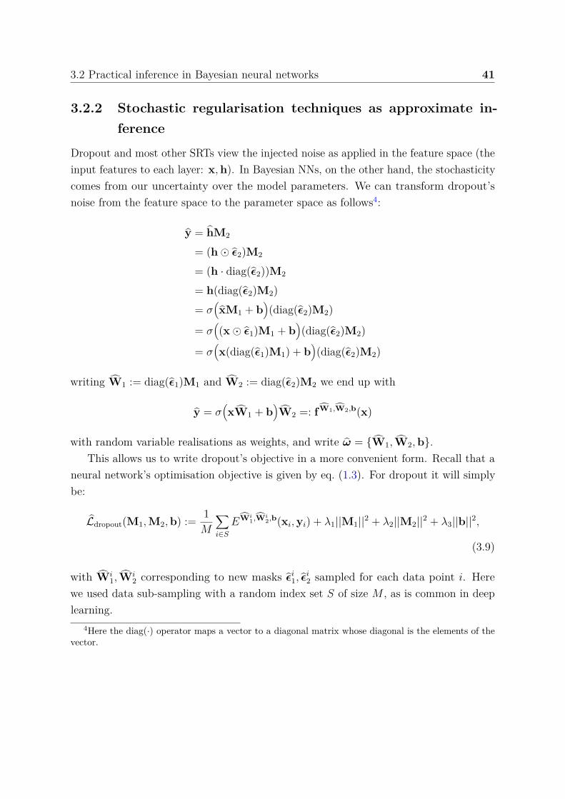
Dropout and most other SRTs view the injected noise as applied in the feature space (the
input features to each layer: x, h). In Bayesian NNs, on the other hand, the stochasticity
comes from our uncertainty over the model parameters. We can transform dropout’s
noise from the feature space to the parameter space as follows4:
y = hM2
= (h⊙ ϵ2)M2
= (h · diag(ϵ2))M2
= h(diag(ϵ2)M2)
= σ(xM1 + b
(diag(ϵ2)M2)
= σ((x⊙ ϵ1)M1 + b
(diag(ϵ2)M2)
= σ(x(diag(ϵ1)M1) + b
(diag(ϵ2)M2)
writing W1 := diag(ϵ1)M1 and W2 := diag(ϵ2)M2 we end up with
y = σ(xW1 + b
W2 =: fW1,W2,b(x)
with random variable realisations as weights, and write ω = ¶W1, W2, b♢.
This allows us to write dropout’s objective in a more convenient form. Recall that a
neural network’s optimisation objective is given by eq. (1.3). For dropout it will simply
be:
Ldropout(M1, M2, b) :=1
M
∑
i∈S
EWi1,Wi
2,b(xi, yi) + λ1♣♣M1♣♣2 + λ2♣♣M2♣♣
2 + λ3♣♣b♣♣2,
(3.9)
with Wi1, Wi
2 corresponding to new masks ϵi1, ϵ
i2 sampled for each data point i. Here
we used data sub-sampling with a random index set S of size M , as is common in deep
learning.
4Here the diag(·) operator maps a vector to a diagonal matrix whose diagonal is the elements of thevector.

42 Bayesian Deep Learning
As shown by Tishby et al. [1989], in regression EM1,M2,b(x, y) can be rewritten as
the negative log-likelihood scaled by a constant:
EM1,M2,b(x, y) =1
2♣♣y− fM1,M2,b(x)♣♣2 = −
1
τlog p(y♣fM1,M2,b(x)) + const (3.10)
where p(y♣fM1,M2,b(x)) = N (y; fM1,M2,b(x), τ−1I) with τ−1 observation noise. It is
simple to see that this holds for classification as well (in which case we should set τ = 1).
Recall that ω = ¶W1, W2, b♢ and write
ωi = ¶Wi1, Wi
2, b♢ = ¶diag(ϵi1)M1, diag(ϵi
2)M2, b♢ =: g(θ, ϵi)
with θ = ¶M1, M2, b♢, ϵi1 ∼ p(ϵ1), and ϵ
i2 ∼ p(ϵ2) for 1 ≤ i ≤ N . Here p(ϵl) (l = 1, 2) is
a product of Bernoulli distributions with probabilities 1− pl, from which a realisation
would be a vector of zeros and ones.
We can plug identity (3.10) into objective (3.9) and get
Ldropout(M1, M2, b) = −1
Mτ
∑
i∈S
log p(yi♣fg(θ,ϵi)(x)) + λ1♣♣M1♣♣
2 + λ2♣♣M2♣♣2 + λ3♣♣b♣♣
2
(3.11)
with ϵi realisations of the random variable ϵ.
The derivative of this optimisation objective w.r.t. model parameters θ = ¶M1, M2, b♢
is given by
∂
∂θLdropout(θ) = −
1
Mτ
∑
i∈S
∂
∂θlog p(yi♣f
g(θ,ϵi)(x)) +∂
∂θ
(λ1♣♣M1♣♣
2 + λ2♣♣M2♣♣2 + λ3♣♣b♣♣
2.
The optimisation of a NN with dropout can then be seen as following algorithm 2.
There is a great sense of similarity between algorithm 1 for approximate inference in a
Bayesian NN and algorithm 2 for dropout NN optimisation. Specifically, note the case of a
Bayesian NN with approximating distribution q(ω) s.t. ω = ¶diag(ϵ1)M1, diag(ϵ2)M2, b♢
with p(ϵl) (l = 1, 2) a product of Bernoulli distributions with probability 1− pl (which we
will refer to as a Bernoulli variational distribution or a dropout variational distribution).
The only differences between algorithm 1 and algorithm 2 are
1. the regularisation term derivatives (KL(qθ(ω)♣♣p(ω)) in algo. 1 and λ1♣♣M1♣♣2 +
λ2♣♣M2♣♣2 + λ3♣♣b♣♣
2 in algo. 2),
2. and the scale of ∆θ (multiplied by a constant 1Nτ
in algo. 2).
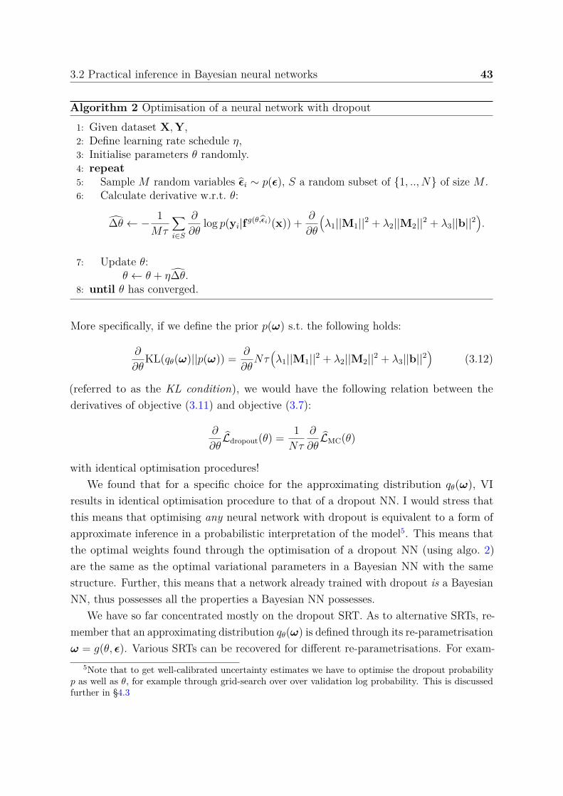
3.2 Practical inference in Bayesian neural networks 43
Algorithm 2 Optimisation of a neural network with dropout
1: Given dataset X, Y,2: Define learning rate schedule η,3: Initialise parameters θ randomly.4: repeat
5: Sample M random variables ϵi ∼ p(ϵ), S a random subset of ¶1, .., N♢ of size M .6: Calculate derivative w.r.t. θ:
∆θ ← −1
Mτ
∑
i∈S
∂
∂θlog p(yi♣f
g(θ,ϵi)(x)) +∂
∂θ
(λ1♣♣M1♣♣
2 + λ2♣♣M2♣♣2 + λ3♣♣b♣♣
2.
7: Update θ:θ ← θ + η∆θ.
8: until θ has converged.
More specifically, if we define the prior p(ω) s.t. the following holds:
∂
∂θKL(qθ(ω)♣♣p(ω)) =
∂
∂θNτ
(λ1♣♣M1♣♣
2 + λ2♣♣M2♣♣2 + λ3♣♣b♣♣
2
(3.12)
(referred to as the KL condition), we would have the following relation between the
derivatives of objective (3.11) and objective (3.7):
∂
∂θLdropout(θ) =
1
Nτ
∂
∂θLMC(θ)
with identical optimisation procedures!
We found that for a specific choice for the approximating distribution qθ(ω), VI
results in identical optimisation procedure to that of a dropout NN. I would stress that
this means that optimising any neural network with dropout is equivalent to a form of
approximate inference in a probabilistic interpretation of the model5. This means that
the optimal weights found through the optimisation of a dropout NN (using algo. 2)
are the same as the optimal variational parameters in a Bayesian NN with the same
structure. Further, this means that a network already trained with dropout is a Bayesian
NN, thus possesses all the properties a Bayesian NN possesses.
We have so far concentrated mostly on the dropout SRT. As to alternative SRTs, re-
member that an approximating distribution qθ(ω) is defined through its re-parametrisation
ω = g(θ, ϵ). Various SRTs can be recovered for different re-parametrisations. For exam-
5Note that to get well-calibrated uncertainty estimates we have to optimise the dropout probabilityp as well as θ, for example through grid-search over over validation log probability. This is discussedfurther in §4.3

44 Bayesian Deep Learning
ple, multiplicative Gaussian noise [Srivastava et al., 2014] can be recovered by setting
g(θ, ϵ) = ¶diag(ϵ1)M1, diag(ϵ2)M2, b♢ with p(ϵl) (for l = 1, 2) a product of N (1, α) with
positive-valued α6. This can be efficiently implemented by multiplying a network’s units
by i.i.d. draws from a N (1, α). On the other hand, setting g(θ, ϵ) = ¶M1⊙ϵ1, M2⊙ϵ2, b♢
with p(ϵl) a product of Bernoulli random variables for each weight scalar we recover
dropConnect [Wan et al., 2013]. This can be efficiently implemented by multiplying a
network’s weight scalars by i.i.d. draws from a Bernoulli distribution. It is interesting
to note that Graves [2011]’s fully factorised approximation can be recovered by setting
g(θ, ϵ) = ¶M1 + ϵ1, M2 + ϵ2, b♢ with p(ϵl) a product of N (0, α) for each weight scalar.
This SRT is often referred to as additive Gaussian noise.
3.2.3 KL condition
For VI to result in an identical optimisation procedure to that of a dropout NN, the KL
condition (eq. (3.12)) has to be satisfied. Under what constraints does the KL condition
hold? This depends on the model specification (selection of prior p(ω)) as well as choice
of approximating distribution qθ(ω). For example, it can be shown that setting the model
prior to p(ω) =∏L
i=1 p(Wi) =∏L
i=1N (0, I/l2i ), in other words independent normal priors
over each weight, with prior length-scale7
l2i =
2Nτλi
1− pi
(3.13)
we have
∂
∂θKL(qθ(ω)♣♣p(ω)) ≈
∂
∂θNτ(λ1♣♣M1♣♣
2 + λ2♣♣M2♣♣2 + λ3♣♣b♣♣
2)
for a large enough number of hidden units and a Bernoulli variational distribution. This
is discussed further in appendix A. Alternatively, a discrete prior distribution
p(w) ∝ e− l2
2wT w
6For the multiplicative Gaussian noise this result was also presented in [Kingma et al., 2015], whichwas done in parallel to this work.
7A note on mean-squared-error losses: the mean-squared-error loss can be seen as a scaling of theEuclidean loss (eq. (1.1)) by a factor of 2, which implies that the factor of 2 in the length-scale shouldbe removed. The mean-squared-error loss is used in many modern deep learning packages instead (or as)the Euclidean loss.
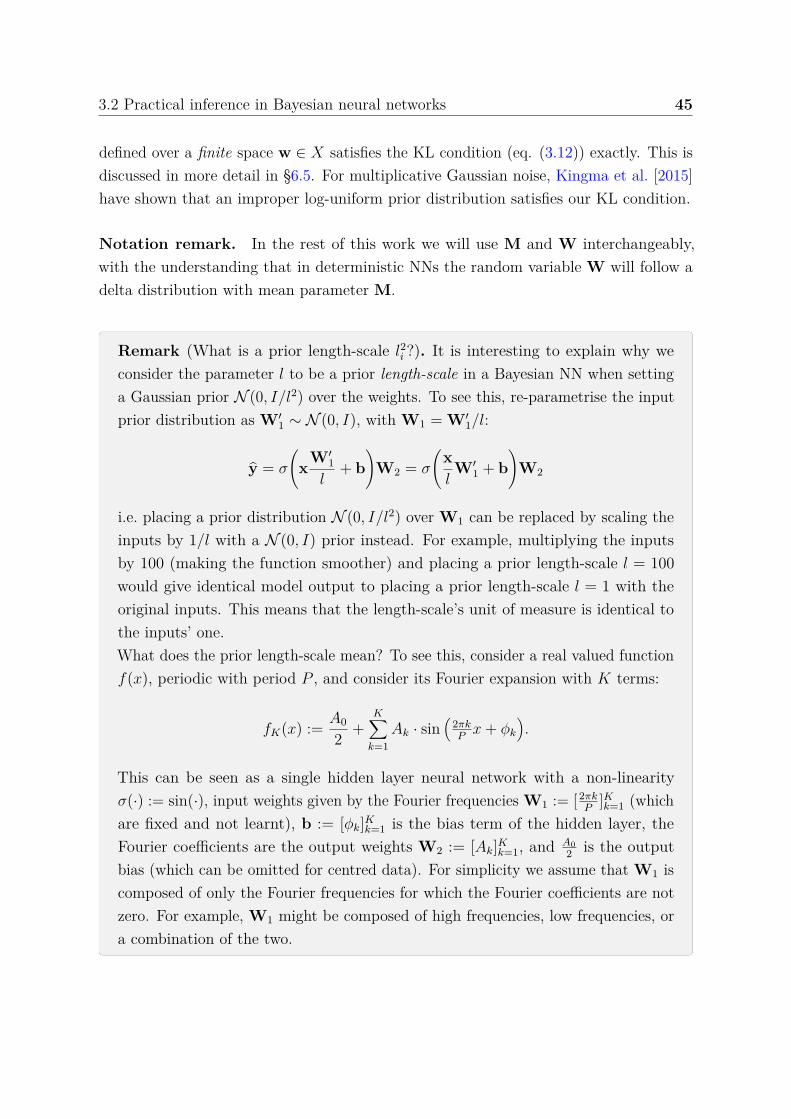
3.2 Practical inference in Bayesian neural networks 45
defined over a finite space w ∈ X satisfies the KL condition (eq. (3.12)) exactly. This is
discussed in more detail in §6.5. For multiplicative Gaussian noise, Kingma et al. [2015]
have shown that an improper log-uniform prior distribution satisfies our KL condition.
Notation remark. In the rest of this work we will use M and W interchangeably,
with the understanding that in deterministic NNs the random variable W will follow a
delta distribution with mean parameter M.
Remark (What is a prior length-scale l2i ?). It is interesting to explain why we
consider the parameter l to be a prior length-scale in a Bayesian NN when setting
a Gaussian prior N (0, I/l2) over the weights. To see this, re-parametrise the input
prior distribution as W′1 ∼ N (0, I), with W1 = W′
1/l:
y = σ
(x
W′1
l+ b
)W2 = σ
(x
lW′
1 + b
)W2
i.e. placing a prior distribution N (0, I/l2) over W1 can be replaced by scaling the
inputs by 1/l with a N (0, I) prior instead. For example, multiplying the inputs
by 100 (making the function smoother) and placing a prior length-scale l = 100
would give identical model output to placing a prior length-scale l = 1 with the
original inputs. This means that the length-scale’s unit of measure is identical to
the inputs’ one.
What does the prior length-scale mean? To see this, consider a real valued function
f(x), periodic with period P , and consider its Fourier expansion with K terms:
fK(x) :=A0
2+
K∑
k=1
Ak · sin(
2πkP
x + ϕk
.
This can be seen as a single hidden layer neural network with a non-linearity
σ(·) := sin(·), input weights given by the Fourier frequencies W1 := [2πkP
]Kk=1 (which
are fixed and not learnt), b := [ϕk]Kk=1 is the bias term of the hidden layer, the
Fourier coefficients are the output weights W2 := [Ak]Kk=1, and A0
2is the output
bias (which can be omitted for centred data). For simplicity we assume that W1 is
composed of only the Fourier frequencies for which the Fourier coefficients are not
zero. For example, W1 might be composed of high frequencies, low frequencies, or
a combination of the two.

46 Bayesian Deep Learning
This view of single hidden layer neural networks gives us some insights into the role
of the different quantities used in a neural network. For example, erratic functions
have high frequencies, i.e. high magnitude input weights W1. On the other hand,
smooth slow-varying functions are composed of low frequencies, and as a result the
magnitude of W1 is small. The magnitude of W2 determines how much different
frequencies will be used to compose the output function fK(x). High magnitude W2
results in a large magnitude for the function’s outputs, whereas low W2 magnitude
gives function outputs scaled down and closer to zero.
When we place a prior distribution over the input weights of a BNN, we can capture
this characteristic. Having W1 ∼ N (0, I/l2) a priori with long length-scale l results
in weights with low magnitude, and as a result slow-varying induced functions. On
the other hand, placing a prior distribution with a short length-scale gives high
magnitude weights, and as a result erratic functions with high frequencies. This
will be demonstrated empirically in §4.1.
Given the intuition about weight magnitude above, equation (3.13) can be re-written
to cast some light on the structure of the weight-decay in a neural networka:
λi =l2i (1− pi)
2Nτ. (3.14)
A short length-scale li (corresponding to high frequency data) with high pre-
cision τ (equivalently, small observation noise) results in a small weight-decay
λi—encouraging the model to fit the data well but potentially generalising badly.
A long length-scale with low precision results in a large weight-decay—and stronger
regularisation over the weights. This trade-off between the length-scale and model
precision results in different weight-decay values.
Lastly, I would comment on the choice of placing a distribution over the rows of a
weight matrix rather than factorising it over each row’s elements. Gal and Turner
[2015] offered a derivation related to the Fourier expansion above, where a function
drawn from a Gaussian process (GP) was approximated through a finite Fourier
decomposition of the GP’s covariance function. This derivation has many properties
in common with the view above. Interestingly, in the multivariate f(x) case the
Fourier frequencies are given in the columns of the equivalent weight matrix W1
of size Q (input dimension) by K (number of expansion terms). This generalises
on the univariate case above where W1 is of dimensions Q = 1 by K and each
entry (column) is a single frequency. Factorising the weight matrix approximating

3.3 Model uncertainty in Bayesian neural networks 47
distribution qθ(W1) over its rows rather than columns captures correlations over
the function’s frequencies.
aNote that with a mean-squared-error loss the factor of 2 should be removed.
3.3 Model uncertainty in Bayesian neural networks
We next derive results extending on the above showing that model uncertainty can be
obtained from NN models that make use of SRTs such as dropout.
Recall that our approximate predictive distribution is given by eq. (2.4):
q∗θ(y∗♣x∗) =
∫p(y∗♣fω(x∗))q∗
θ(ω)dω (3.15)
where ω = ¶Wi♢Li=1 is our set of random variables for a model with L layers, fω(x∗) is
our model’s stochastic output, and q∗θ(ω) is an optimum of eq. (3.7).
We will perform moment-matching and estimate the first two moments of the predictive
distribution empirically. The first moment can be estimated as follows:
Proposition 2. Given p(y∗♣fω(x∗)) = N (y∗; fω(x∗), τ−1I) for some τ > 0, Eq∗
θ(y∗♣x∗)[y
∗]
can be estimated with the unbiased estimator
E[y∗] :=1
T
T∑
t=1
f ωt(x∗) −−−→T →∞
Eq∗
θ(y∗♣x∗)[y
∗] (3.16)
with ωt ∼ q∗θ(ω).
Proof.
Eq∗
θ(y∗♣x∗)[y
∗] =∫
y∗q∗θ(y∗♣x∗)dy∗
=∫ ∫
y∗N (y∗; fω(x∗), τ−1I)q∗θ(ω)dωdy∗
=∫ ( ∫
y∗N (y∗; fω(x∗), τ−1I)dy∗
)q∗
θ(ω)dω
=∫
fω(x∗)q∗θ(ω)dω,
giving the unbiased estimator E[y∗] := 1T
∑Tt=1 f ωt(x∗) following MC integration with T
samples.
48 Bayesian Deep Learning
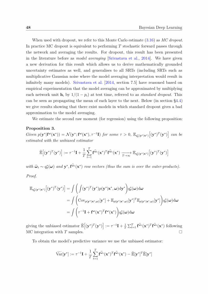
When used with dropout, we refer to this Monte Carlo estimate (3.16) as MC dropout.
In practice MC dropout is equivalent to performing T stochastic forward passes through
the network and averaging the results. For dropout, this result has been presented
in the literature before as model averaging [Srivastava et al., 2014]. We have given
a new derivation for this result which allows us to derive mathematically grounded
uncertainty estimates as well, and generalises to all SRTs (including SRTs such as
multiplicative Gaussian noise where the model averaging interpretation would result in
infinitely many models). Srivastava et al. [2014, section 7.5] have reasoned based on
empirical experimentation that the model averaging can be approximated by multiplying
each network unit hi by 1/(1− pi) at test time, referred to as standard dropout. This
can be seen as propagating the mean of each layer to the next. Below (in section §4.4)
we give results showing that there exist models in which standard dropout gives a bad
approximation to the model averaging.
We estimate the second raw moment (for regression) using the following proposition:
Proposition 3.
Given p(y∗♣fω(x∗)) = N (y∗; fω(x∗), τ−1I) for some τ > 0, Eq∗
θ(y∗♣x∗)
[(y∗)T (y∗)
]can be
estimated with the unbiased estimator
E
[(y∗)T (y∗)
]:= τ−1I +
1
T
T∑
t=1
f ωt(x∗)T f ωt(x∗) −−−→T →∞
Eq∗
θ(y∗♣x∗)
[(y∗)T (y∗)
]
with ωt ∼ q∗θ(ω) and y∗, f ωt(x∗) row vectors (thus the sum is over the outer-products).
Proof.
Eq∗
θ(y∗♣x∗)
[(y∗)T (y∗)
]=∫ ( ∫
(y∗)T (y∗)p(y∗♣x∗, ω)dy∗
)q∗
θ(ω)dω
=∫ (
Covp(y∗♣x∗,ω)[y∗] + Ep(y∗♣x∗,ω)[y
∗]TEp(y∗♣x∗,ω)[y∗]
)q∗
θ(ω)dω
=∫ (
τ−1I + fω(x∗)T fω(x∗)
)q∗
θ(ω)dω
giving the unbiased estimator E
[(y∗)T (y∗)
]:= τ−1I + 1
T
∑Tt=1 f ωt(x∗)T f ωt(x∗) following
MC integration with T samples.
To obtain the model’s predictive variance we use the unbiased estimator:
Var[y∗] := τ−1I +1
T
T∑
t=1
f ωt(x∗)T f ωt(x∗)− E[y∗]T E[y∗]

3.3 Model uncertainty in Bayesian neural networks 49
−−−→T →∞
Varq∗
θ(y∗♣x∗)[y
∗]
which equals the sample variance of T stochastic forward passes through the NN plus
the inverse model precision.
How can we find the model precision? In practice in the deep learning literature we
often grid-search over the weight-decay λ to minimise validation error. Then, given a
weight-decay λi (and prior length-scale li), eq. (3.13) can be re-written to find the model
precision8:
τ =(1− p)l2
i
2Nλi
. (3.17)
Remark (Predictive variance and posterior variance). It is important to note the
difference between the variance of the approximating distribution qθ(ω) and the
variance of the predictive distribution qθ(y♣x) (eq. (3.15)).
To see this, consider the illustrative example of an approximating distribution
with fixed mean and variance used with the first weight layer W1, for example a
standard Gaussian N (0, I). Further, assume for the sake of argument that delta
distributions (or Gaussians with very small variances) are used to approximate the
posterior over the layers following the first layer. Given enough follow-up layers we
can capture any function to arbitrary precision—including the inverse cumulative
distribution function (CDF) of any distribution (similarly to the remark in §2.2.1,
but with the addition of a Gaussian CDF as we don’t have a uniform on the first
layer in this case). Passing the distribution from the first layer through the rest of
the layers transforms the standard Gaussian with this inverse CDF, resulting in
any arbitrary distribution as determined by the CDF.
In this example, even though the variance of each weight layer is constant, the
variance of the predictive distribution can take any value depending on the learnt
CDF. This example can be extended from a standard Gaussian approximating
distribution to a mixture of Gaussians with fixed standard deviations, and to discrete
distributions with fixed probability vectors (such as the dropout approximating
distribution). Of course, in real world cases we would prefer to avoid modelling the
8Prior length-scale li can be fixed based on the density of the input data X and our prior belief as tothe function’s wiggliness, or optimised over as well (w.r.t. predictive log-likelihood over a validation set).The dropout probability is optimised using grid search similarly.

50 Bayesian Deep Learning
deep layers with delta approximating distributions since that would sacrifice our
ability to capture model uncertainty.
Given a dataset X, Y and a new data point x∗ we can calculate the probability
of possible output values y∗ using the predictive probability p(y∗♣x∗, X, Y). The log
of the predictive likelihood captures how well the model fits the data, with larger
values indicating better model fit. Our predictive log-likelihood (also referred to as test
log-likelihood) can be approximated by MC integration of eq. (3.15) with T terms:
˜log p(y∗♣x∗, X, Y) := log
(1
T
T∑
t=1
p(y∗♣x∗, ωt)
)−−−→T →∞
log∫
p(y∗♣x∗, ω)q∗θ(ω)dω
≈ log∫
p(y∗♣x∗, ω)p(ω♣X, Y)dω
= log p(y∗♣x∗, X, Y)
with ωt ∼ q∗θ(ω) and since q∗
θ(ω) is the minimiser of eq. (2.3). Note that this is a
biased estimator since the expected quantity is transformed with the non-linear logarithm
function, but the bias decreases as T increases.
For regression we can rewrite this last equation in a more numerically stable way9:
˜log p(y∗♣x∗, X, Y) = logsumexp
(−
1
2τ ♣♣y− f ωt(x∗)♣♣2
)− log T −
1
2log 2π +
1
2log τ
(3.18)
with our precision parameter τ .
Uncertainty quality can be determined from this quantity as well. Excessive un-
certainty (large observation noise, or equivalently small model precision τ) results in
a large penalty from the last term in the predictive log-likelihood. On the other hand,
an over-confident model with large model precision compared to poor mean estimation
results in a penalty from the first term—the distance ♣♣y− f ωt(x∗)♣♣2 gets amplified by τ
which drives the exponent to zero.
Note that the normal NN model itself is not changed. To estimate the predictive
mean and predictive uncertainty we simply collect the results of stochastic forward passes
through the model. As a result, this information can be used with existing NN models
trained with SRTs. Furthermore, the forward passes can be done concurrently, resulting
in constant running time identical to that of standard NNs.
9logsumexp is the log-sum-exp function.
3.3 Model uncertainty in Bayesian neural networks 51
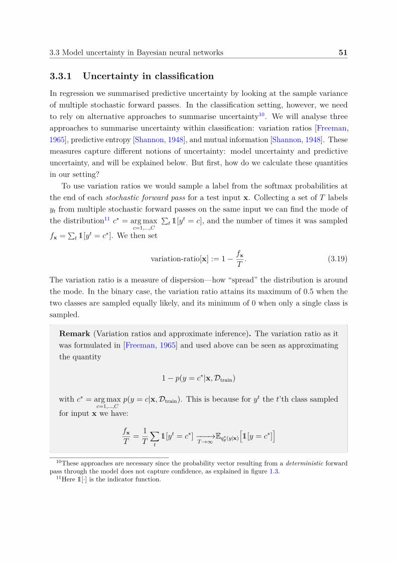
3.3.1 Uncertainty in classification
In regression we summarised predictive uncertainty by looking at the sample variance
of multiple stochastic forward passes. In the classification setting, however, we need
to rely on alternative approaches to summarise uncertainty10. We will analyse three
approaches to summarise uncertainty within classification: variation ratios [Freeman,
1965], predictive entropy [Shannon, 1948], and mutual information [Shannon, 1948]. These
measures capture different notions of uncertainty: model uncertainty and predictive
uncertainty, and will be explained below. But first, how do we calculate these quantities
in our setting?
To use variation ratios we would sample a label from the softmax probabilities at
the end of each stochastic forward pass for a test input x. Collecting a set of T labels
yt from multiple stochastic forward passes on the same input we can find the mode of
the distribution11 c∗ = arg maxc=1,...,C
∑t 1[yt = c], and the number of times it was sampled
fx =∑
t 1[yt = c∗]. We then set
variation-ratio[x] := 1−fx
T. (3.19)
The variation ratio is a measure of dispersion—how “spread” the distribution is around
the mode. In the binary case, the variation ratio attains its maximum of 0.5 when the
two classes are sampled equally likely, and its minimum of 0 when only a single class is
sampled.
Remark (Variation ratios and approximate inference). The variation ratio as it
was formulated in [Freeman, 1965] and used above can be seen as approximating
the quantity
1− p(y = c∗♣x,Dtrain)
with c∗ = arg maxc=1,...,C
p(y = c♣x,Dtrain). This is because for yt the t’th class sampled
for input x we have:
fx
T=
1
T
∑
t
1[yt = c∗] −−−→T →∞
Eq∗
θ(y♣x)
[1[y = c∗]
]
10These approaches are necessary since the probability vector resulting from a deterministic forwardpass through the model does not capture confidence, as explained in figure 1.3.
11Here 1[·] is the indicator function.

52 Bayesian Deep Learning
=q∗θ(y = c∗♣x)
≈p(y = c∗♣x,Dtrain)
and,
c∗ = arg maxc=1,...,C
∑
t
1[yt = c] =arg maxc=1,...,C
1
T
∑
t
1[yt = c]
−−−→T →∞
arg maxc=1,...,C
Eq∗
θ(y♣x)[1[y = c]]
=arg maxc=1,...,C
q∗θ(y = c♣x).
≈arg maxc=1,...,C
p(y = c♣x,Dtrain)
since q∗θ(ω) is a minimiser of the KL divergence to p(ω♣Dtrain) and therefore
q∗θ(y♣x) ≈
∫p(y♣fω(x))p(ω♣Dtrain)dω (following eq. (3.15)).
Unlike variation ratios, predictive entropy has its foundations in information theory.
This quantity captures the average amount of information contained in the predictive
distribution:
H[y♣x,Dtrain] := −∑
c
p(y = c♣x,Dtrain) log p(y = c♣x,Dtrain) (3.20)
summing over all possible classes c that y can take. Given a test point x, the predictive
entropy attains its maximum value when all classes are predicted to have equal uniform
probability, and its minimum value of zero when one class has probability 1 and all others
probability 0 (i.e. the prediction is certain).
In our setting, the predictive entropy can be approximated by collecting the probability
vectors from T stochastic forward passes through the network, and for each class c
averaging the probabilities of the class from each of the T probability vectors, replacing
p(y = c♣x,Dtrain) in eq. (3.20). In other words, we replace p(y = c♣x,Dtrain) with1T
∑t p(y = c♣x, ωt), where p(y = c♣x, ωt) is the probability of input x to take class c
with model parameters ωt ∼ q∗θ(ω):
[p(y = 1♣x, ωt), ..., p(y = C♣x, ωt)] := Softmax(f ωt(x)).
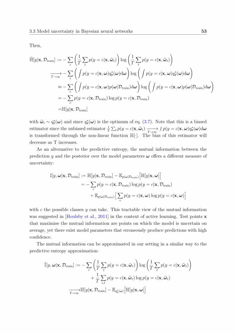
3.3 Model uncertainty in Bayesian neural networks 53
Then,
H[y♣x,Dtrain] :=−∑
c
(1
T
∑
t
p(y = c♣x, ωt)
)log
(1
T
∑
t
p(y = c♣x, ωt)
)
−−−→T →∞
−∑
c
(∫p(y = c♣x, ω)q∗
θ(ω)dω
)log
(∫p(y = c♣x, ω)q∗
θ(ω)dω
)
≈−∑
c
(∫p(y = c♣x, ω)p(ω♣Dtrain)dω
)log
(∫p(y = c♣x, ω)p(ω♣Dtrain)dω
)
=−∑
c
p(y = c♣x,Dtrain) log p(y = c♣x,Dtrain)
=H[y♣x,Dtrain]
with ωt ∼ q∗θ(ω) and since q∗
θ(ω) is the optimum of eq. (3.7). Note that this is a biased
estimator since the unbiased estimator 1T
∑t p(y = c♣x, ωt) −−−→
T →∞
∫p(y = c♣x, ω)q∗
θ(ω)dω
is transformed through the non-linear function H[·]. The bias of this estimator will
decrease as T increases.
As an alternative to the predictive entropy, the mutual information between the
prediction y and the posterior over the model parameters ω offers a different measure of
uncertainty:
I[y, ω♣x,Dtrain] := H[y♣x,Dtrain]− Ep(ω♣Dtrain)
[H[y♣x, ω]
]
= −∑
c
p(y = c♣x,Dtrain) log p(y = c♣x,Dtrain)
+ Ep(ω♣Dtrain)
[∑
c
p(y = c♣x, ω) log p(y = c♣x, ω)]
with c the possible classes y can take. This tractable view of the mutual information
was suggested in [Houlsby et al., 2011] in the context of active learning. Test points x
that maximise the mutual information are points on which the model is uncertain on
average, yet there exist model parameters that erroneously produce predictions with high
confidence.
The mutual information can be approximated in our setting in a similar way to the
predictive entropy approximation:
I[y, ω♣x,Dtrain] :=−∑
c
(1
T
∑
t
p(y = c♣x, ωt)
)log
(1
T
∑
t
p(y = c♣x, ωt)
)
+1
T
∑
c,t
p(y = c♣x, ωt) log p(y = c♣x, ωt)
−−−→T →∞
H[y♣x,Dtrain]− Eq∗
θ(ω)
[H[y♣x, ω]
]
54 Bayesian Deep Learning
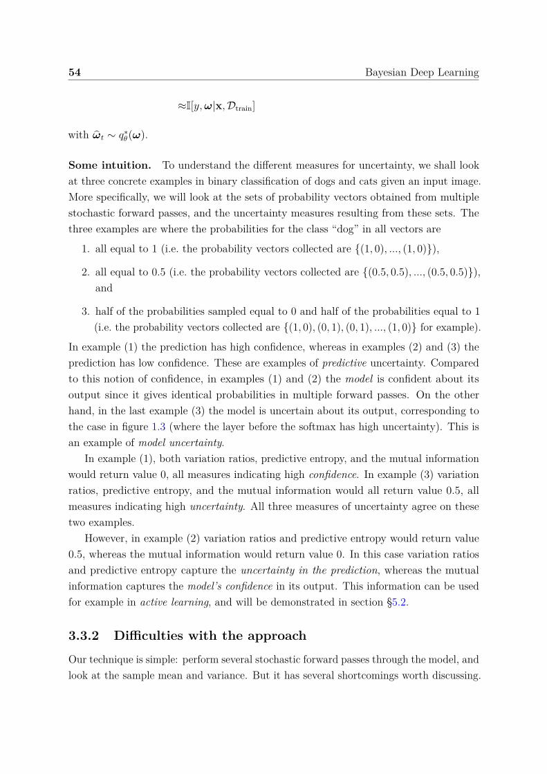
≈I[y, ω♣x,Dtrain]
with ωt ∼ q∗θ(ω).
Some intuition. To understand the different measures for uncertainty, we shall look
at three concrete examples in binary classification of dogs and cats given an input image.
More specifically, we will look at the sets of probability vectors obtained from multiple
stochastic forward passes, and the uncertainty measures resulting from these sets. The
three examples are where the probabilities for the class “dog” in all vectors are
1. all equal to 1 (i.e. the probability vectors collected are ¶(1, 0), ..., (1, 0)♢),
2. all equal to 0.5 (i.e. the probability vectors collected are ¶(0.5, 0.5), ..., (0.5, 0.5)♢),
and
3. half of the probabilities sampled equal to 0 and half of the probabilities equal to 1
(i.e. the probability vectors collected are ¶(1, 0), (0, 1), (0, 1), ..., (1, 0)♢ for example).
In example (1) the prediction has high confidence, whereas in examples (2) and (3) the
prediction has low confidence. These are examples of predictive uncertainty. Compared
to this notion of confidence, in examples (1) and (2) the model is confident about its
output since it gives identical probabilities in multiple forward passes. On the other
hand, in the last example (3) the model is uncertain about its output, corresponding to
the case in figure 1.3 (where the layer before the softmax has high uncertainty). This is
an example of model uncertainty.
In example (1), both variation ratios, predictive entropy, and the mutual information
would return value 0, all measures indicating high confidence. In example (3) variation
ratios, predictive entropy, and the mutual information would all return value 0.5, all
measures indicating high uncertainty. All three measures of uncertainty agree on these
two examples.
However, in example (2) variation ratios and predictive entropy would return value
0.5, whereas the mutual information would return value 0. In this case variation ratios
and predictive entropy capture the uncertainty in the prediction, whereas the mutual
information captures the model’s confidence in its output. This information can be used
for example in active learning, and will be demonstrated in section §5.2.
3.3.2 Difficulties with the approach
Our technique is simple: perform several stochastic forward passes through the model, and
look at the sample mean and variance. But it has several shortcomings worth discussing.
3.3 Model uncertainty in Bayesian neural networks 55
First, even though the training time of our model is identical to that of existing models
in the field, the test time is scaled by T—the number of averaged forward passes through
the network. This may not be of real concern in some real world applications, as NNs are
often implemented on distributed hardware. Distributed hardware allows us to obtain
MC estimates in constant time almost trivially, by transferring an input to a GPU and
setting a mini-batch composed of the same input multiple times. In dropout for example
we sample different Bernoulli realisations for each output unit and each mini-batch input,
which results in a matrix of probabilities. Each row in the matrix is the output of the
dropout network on the same input generated with different random variable realisations
(dropout masks). Averaging over the rows results in the MC dropout estimate.
Another concern is that the model’s uncertainty is not calibrated. A calibrated
model is one in which the predictive probabilities match the empirical frequency of the
data. The lack of calibration can be seen through the derivation’s relation to Gaussian
processes [Gal and Ghahramani, 2015b]. Gaussian processes’ uncertainty is known
to not be calibrated—the Gaussian process’s uncertainty depends on the covariance
function chosen, which is shown in [Gal and Ghahramani, 2015b] to be equivalent to
the non-linearities and prior over the weights. The choice of a GP’s covariance function
follows from our assumptions about the data. If we believe, for example, that the model’s
uncertainty should increase far from the data we might choose the squared exponential
covariance function.
For many practical applications the lack of calibration means that model uncertainty
can increase for large magnitude data points or be of different scale for different datasets.
To calibrate model uncertainty in regression tasks we can scale the uncertainty linearly
to remove data magnitude effects, and manipulate uncertainty percentiles to compare
among different datasets. This can be done by finding the number of validation set
points having larger uncertainty than that of a test point. For example, if a test point
has predictive standard deviation 5, whereas almost all validation points have standard
deviation ranging from 0.2 to 2, then the test point’s uncertainty value will be in the top
percentile of the validation set uncertainty measures, and the model will be considered as
very uncertain about the test point compared to the validation data. However, another
model might give the same test point predictive standard deviation of 5 with most of
the validation data given predictive standard deviation ranging from 10 to 15. In this
model the test point’s uncertainty measure will be in the lowest percentile of validation
set uncertainty measures, and the model will be considered as fairly confident about the
test point with respect to the validation data.

56 Bayesian Deep Learning
One last concern is a known limitation of VI. Variational inference is known to
underestimates predictive variance [Turner and Sahani, 2011], a property descendent
from our objective (which penalises qθ(ω) for placing mass where p(ω♣X, Y) has no
mass, but less so for not placing mass where it should). Several solutions exist for
this (such as [Giordano et al., 2015]), with different limitations for their practicality.
Uncertainty under-estimation does not seem to be of real concern in practice though,
and the variational approximation seems to work well in practical applications as we will
see in the next chapter.
3.4 Approximate inference in complex models
We finish the chapter by extending the approximate inference technique above to more
complex models such as convolutional neural networks and recurrent neural networks.
This will allow us to obtain model uncertainty for models defined over sequence based
datasets or for image data. We describe the approximate inference using Bernoulli
variational distributions for convenience of presentation, although any SRT could be used
instead.
3.4.1 Bayesian convolutional neural networks
In existing convolutional neural networks (CNNs) literature dropout is mostly used after
inner-product layers at the end of the model alone. This can be seen as applying a
finite deterministic transformation to the data before feeding it into a Bayesian NN.
As such, model uncertainty can still be obtained for such models, but an interesting
question is whether we could use approximate Bayesian inference over the full CNN.
Here we wish to integrate over the convolution layers (kernels) of the CNN as well. To
implement a Bayesian CNN we could apply dropout after all convolution layers as well
as inner-product layers, and evaluate the model’s predictive posterior using eq. (3.8) at
test time. Note though that generalisations to SRTs other than dropout are also possible
and easy to implement.
Recall the structure of a CNN described in §1.1 and in figure 1.1. In more de-
tail, the input to the i’th convolution layer is represented as a 3 dimensional tensor
x ∈ RHi−1×Wi−1×Ki−1 with height Hi−1, width Wi−1, and Ki−1 channels. A convolution
layer is then composed of a sequence of Ki kernels (weight tensors): kk ∈ Rh×w×Ki−1
for k = 1, ..., Ki. Here we assume kernel height h, kernel width w, and the last di-
mension to match the number of channels in the input layer: Ki−1. Convolving
3.4 Approximate inference in complex models 57
the kernels with the input (with a given stride s) then results in an output layer
of dimensions y ∈ RH′
i−1×W ′
i−1×Ki with H ′i−1 and W ′
i−1 being the new height and
width, and Ki channels—the number of kernels. Each element yi,j,k is the sum of
the element-wise product of kernel kk with a corresponding patch in the input image x:
[[xi−h/2,j−w/2,1, ..., xi+h/2,j+w/2,1], ..., [xi−h/2,j−w/2,Ki−1, ..., xi+h/2,j+w/2,Ki−1
]].
To integrate over the kernels, we reformulate the convolution as a linear operation. Let
kk ∈ Rh×w×Ki−1 for k = 1, ..., Ki be the CNN’s kernels with height h, width w, and Ki−1
channels in the i’th layer. The input to the layer is represented as a 3 dimensional tensor
x ∈ RHi−1×Wi−1×Ki−1 with height Hi−1, width Wi−1, and Ki−1 channels. Convolving the
kernels with the input with a given stride s is equivalent to extracting patches from the
input and performing a matrix product: we extract h× w ×Ki−1 dimensional patches
from the input with stride s and vectorise these. Collecting the vectors in the rows of
a matrix we obtain a new representation for our input x ∈ Rn×hwKi−1 with n patches.
The vectorised kernels form the columns of the weight matrix Wi ∈ RhwKi−1×Ki. The
convolution operation is then equivalent to the matrix product xWi ∈ Rn×Ki. The
columns of the output can be re-arranged into a 3 dimensional tensor y ∈ RHi×Wi×Ki
(since n = Hi ×Wi). Pooling can then be seen as a non-linear operation on the matrix y.
Note that the pooling operation is a non-linearity applied after the linear convolution
counterpart to ReLU or Tanh non-linearities.
To make the CNN into a probabilistic model we place a prior distribution over each
kernel and approximately integrate each kernels-patch pair with Bernoulli variational
distributions. We sample Bernoulli random variables ϵi,j,n and multiply patch n by
the weight matrix Wi · diag([ϵi,j,n]Ki
j=1). This product is equivalent to an approximating
distribution modelling each kernel-patch pair with a distinct random variable, tying
the means of the random variables over the patches. The distribution randomly sets
kernels to zero for different patches. This approximating distribution is also equivalent
to applying dropout for each element in the tensor y before pooling. Implementing our
Bayesian CNN is therefore as simple as using dropout after every convolution layer before
pooling.
The standard dropout test time approximation (scaling hidden units by 1/(1− pi))
does not perform well when dropout is applied after convolutions—this is a negative result
we identified empirically. We solve this by approximating the predictive distribution
following eq. (3.8), averaging stochastic forward passes through the model at test time
(using MC dropout). We assess the model above with an extensive set of experiments
studying its properties in §4.4.

58 Bayesian Deep Learning
3.4.2 Bayesian recurrent neural networks
We next develop inference with Bernoulli variational distributions for recurrent neural
networks (RNNs), although generalisations to SRTs other than dropout are trivial. We
will concentrate on simple RNN models for brevity of notation. Derivations for LSTM
and GRU follow similarly. Given input sequence x = [x1, ..., xT ] of length T , a simple
RNN is formed by a repeated application of a deterministic function fh. This generates a
hidden state ht for time step t:
ht = fh(xt, ht−1) = σ(xtWh + ht−1Uh + bh)
for some non-linearity σ. The model output can be defined, for example, as
fy(hT ) = hT Wy + by.
To view this RNN as a probabilistic model we regard ω = ¶Wh, Uh, bh, Wy, by♢ as
random variables (following Gaussian prior distributions). To make the dependence on
ω clear, we write fω
y for fy and similarly for fω
h . We define our probabilistic model’s
likelihood as above (section 2.1). The posterior over random variables ω is rather complex,
and we approximate it with a variational distribution q(ω). For the dropout SRT for
example we may use a Bernoulli approximating distribution.
Recall our VI optimisation objective eq. (3.1). Evaluating each log likelihood term in
eq. (3.1) with our RNN model we have
∫q(ω) log p(y♣fω
y (hT ))dω =∫
q(ω) log p
(y
∣∣∣∣∣fω
y
(fω
h (xT , hT −1))
dω
=∫
q(ω) log p
(y
∣∣∣∣∣fω
y
(fω
h (xT , fω
h (...fω
h (x1, h0)...)))
dω
with h0 = 0. We approximate this with MC integration with a single sample:
≈ log p
(y
∣∣∣∣∣fω
y
(f ω
h (xT , f ω
h (...f ω
h (x1, h0)...)))
,
with ω ∼ q(ω), resulting in an unbiased estimator to each sum term12.
12Note that for brevity we did not re-parametrise the integral, although this should be done to obtainlow variance derivative estimators.

3.4 Approximate inference in complex models 59
This estimator is plugged into equation (3.1) to obtain our minimisation objective
LMC = −N∑
i=1
log p
(yi
∣∣∣∣∣fωiy
(f ωi
h (xi,T , f ωi
h (...f ωi
h (xi,1, h0)...)))
+ KL(q(ω)♣♣p(ω)). (3.21)
Note that for each sequence xi we sample a new realisation ωi = ¶Wih, Ui
h, bih, Wi
y, biy♢,
and that each symbol in the sequence xi = [xi,1, ..., xi,T ] is passed through the function
f ωi
h with the same weight realisations Wih, Ui
h, bih used at every time step t ≤ T .
In the dropout case, evaluating the model output f ω
y (·) with sample ω corresponds to
randomly zeroing (masking) rows in each weight matrix W during the forward pass. In
our RNN setting with a sequence input, each weight matrix row is randomly masked
once, and importantly the same mask is used through all time steps. When viewed as a
stochastic regularisation technique, our induced dropout variant is therefore identical
to implementing dropout in RNNs with the same network units dropped at each time
step, randomly dropping inputs, outputs, and recurrent connections. Predictions can be
approximated by either propagating the mean of each layer to the next (referred to as the
standard dropout approximation), or by performing dropout at test time and averaging
results (MC dropout, eq. (3.16)).
Remark (Bayesian versus ensembling interpretation of dropout). Apart from our
Bayesian approximation interpretation, dropout in deep networks can also be seen as
following an ensembling interpretation [Srivastava et al., 2014]. This interpretation
also leads to MC dropout at test time. But the ensembling interpretation does
not determine whether the ensemble should be over the network units or the
weights. For example, in an RNN this view will not lead to our dropout variant,
unless the ensemble is defined to tie the weights of the network ad hoc. This is in
comparison to the Bayesian approximation view where the weight tying is forced
by the probabilistic interpretation of the model.
The same can be said about the latent variable model view of dropout [Maeda,
2014] where a constraint over the weights would have to be added ad hoc to derive
the results presented here.
Certain RNN models such as LSTMs [Graves et al., 2013; Hochreiter and Schmidhuber,
1997] and GRUs [Cho et al., 2014] use different gates within the RNN units. For example,
an LSTM is defined by setting four gates: “input”, “forget”, “output”, and an “input
modulation gate”,
i = sigm(ht−1Ui + xtWi
f = sigm
(ht−1Uf + xtWf

60 Bayesian Deep Learning
o = sigm(ht−1Uo + xtWo
g = tanh
(ht−1Ug + xtWg
ct = f ⊙ ct−1 + i⊙ g ht = o⊙ tanh(ct) (3.22)
with ω = ¶Wi, Ui, Wf , Uf , Wo, Uo, Wg, Ug♢ weight matrices and sigm the sigmoid
non-linearity. Here an internal state ct (also referred to as cell) is updated additively.
Alternatively, the model could be re-parametrised as in [Graves et al., 2013]:
i
f
o
g
=
sigm
sigm
sigm
tanh
W ·
xt
ht−1
(3.23)
with ω = ¶W♢, W = [Wi, Ui; Wf , Uf ; Wo, Uo; Wg, Ug] a matrix of dimensions 4K by
2K (K being the dimensionality of xt). We name this parametrisation a tied-weights
LSTM (compared to the untied-weights LSTM parametrisation in eq. (3.22)).
Even though these two parametrisations result in the same deterministic model output,
they lead to different approximating distributions q(ω). With the first parametrisation
one could use different dropout masks for different gates (even when the same input xt is
used). This is because the approximating distribution is placed over the matrices rather
than the inputs: we might drop certain rows in one weight matrix W applied to xt and
different rows in another matrix W′ applied to xt. With the second parametrisations we
would place a distribution over the single matrix W. This leads to a faster forward-pass,
but with slightly diminished results (this tradeoff is examined in section §4.5).
Remark (Word embeddings dropout). In datasets with continuous inputs we often
apply SRTs such as dropout to the input layer—i.e. to the input vector itself. This
is equivalent to placing a distribution over the weight matrix which follows the
input and approximately integrating over it (the matrix is optimised, therefore
prone to overfitting otherwise).
But for models with discrete inputs such as words (where every word is mapped to a
continuous vector—a word embedding)—this is seldom done. With word embeddings
the input can be seen as either the word embedding itself, or, more conveniently, as
a “one-hot” encoding (a vector of zeros with 1 at a single position). The product of
the one-hot encoded vector with an embedding matrix WE ∈ RV ×D (where D is
the embedding dimensionality and V is the number of words in the vocabulary)
then gives a word embedding. Curiously, this parameter layer is the largest layer in

3.4 Approximate inference in complex models 61
most language applications, yet it is often not regularised. Since the embedding
matrix is optimised it can lead to overfitting, and it is therefore desirable to apply
dropout to the one-hot encoded vectors. This in effect is identical to dropping
words at random throughout the input sentence, and can also be interpreted as
encouraging the model to not “depend” on single words for its output.
Note that as before, we randomly set rows of the matrix WE ∈ RV ×D to zero. Since
we repeat the same mask at each time step, we drop the same words throughout
the sequence—i.e. we drop word types at random rather than word tokens (as an
example, the sentence “the dog and the cat” might become “— dog and — cat”
or “the — and the cat”, but never “— dog and the cat”). A possible inefficiency
implementing this is the requirement to sample V Bernoulli random variables,
where V might be large. This can be solved by the observation that for sequences
of length T , at most T embeddings could be dropped (other dropped embeddings
have no effect on the model output). For T ≪ V it is therefore more efficient
to first map the words to the word embeddings, and only then to zero-out word
embeddings based on their word type.
F • f
In the next chapter we will study the techniques above empirically and analyse
them quantitatively. This is followed by a survey of recent literature making use of
the techniques in real-world problems concerning AI safety, image processing, sequence
processing, active learning, and other examples.