Bayesian Decision Theory - ntnu.edu.tw
60
Bayesian Decision Theory References: 1. E. Alpaydin, Introduction to Machine Learning , Chapter 3 2. Tom M. Mitchell, Machine Learning, Chapter 6 Berlin Chen 2005
Transcript of Bayesian Decision Theory - ntnu.edu.tw

Bayesian Decision Theory
References:1. E. Alpaydin, Introduction to Machine Learning , Chapter 32. Tom M. Mitchell, Machine Learning, Chapter 6
Berlin Chen 2005
MLDM-Berlin Chen 2
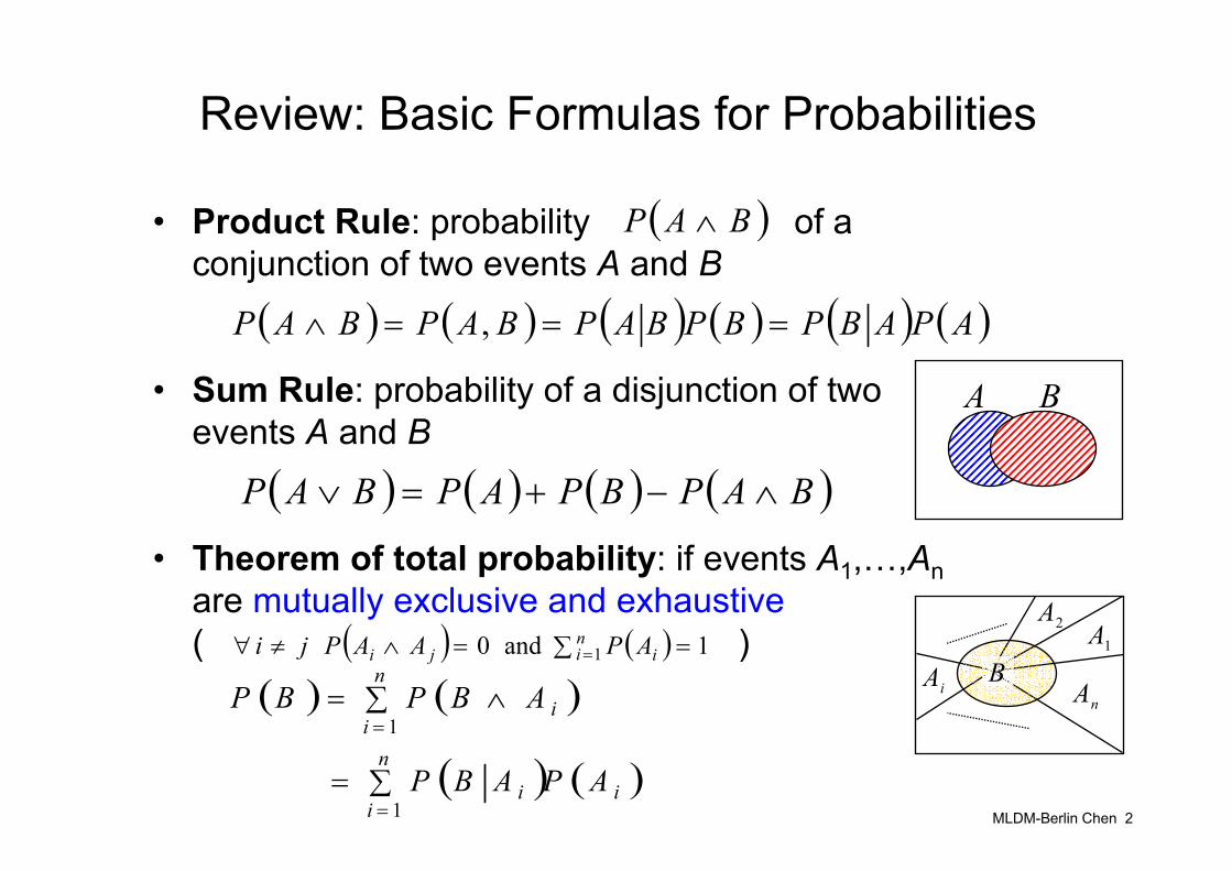
Review: Basic Formulas for Probabilities
• Product Rule: probability of a conjunction of two events A and B
• Sum Rule: probability of a disjunction of twoevents A and B
• Theorem of total probability: if events A1,…,Anare mutually exclusive and exhaustive( )
( )BAP ∧
( ) ( ) ( ) ( ) ( ) ( )APABPBPBAPBAPBAP ===∧ ,
( ) ( )
( ) ( )in
ii
n
ii
APABP
ABPBP
∑=
∑ ∧=
=
=
1
1
( ) ( )∑ ==∧≠∀ =ni iji APAAPji 1 1 and 0
( ) ( ) ( ) ( )BAPBPAPBAP ∧−+=∨
A B
1A2A
iAnA
B
MLDM-Berlin Chen 3
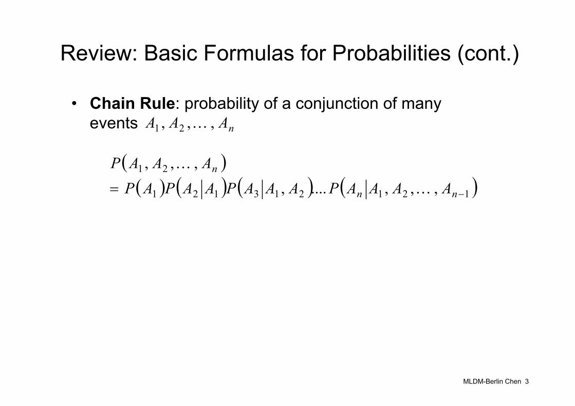
Review: Basic Formulas for Probabilities (cont.)
• Chain Rule: probability of a conjunction of manyevents nAAA ,,, 21 K
( )( ) ( ) ( ) ( )121213121
21
,,,....,,,,
−= nn
n
AAAAPAAAPAAPAPAAAP
K
K
MLDM-Berlin Chen 4
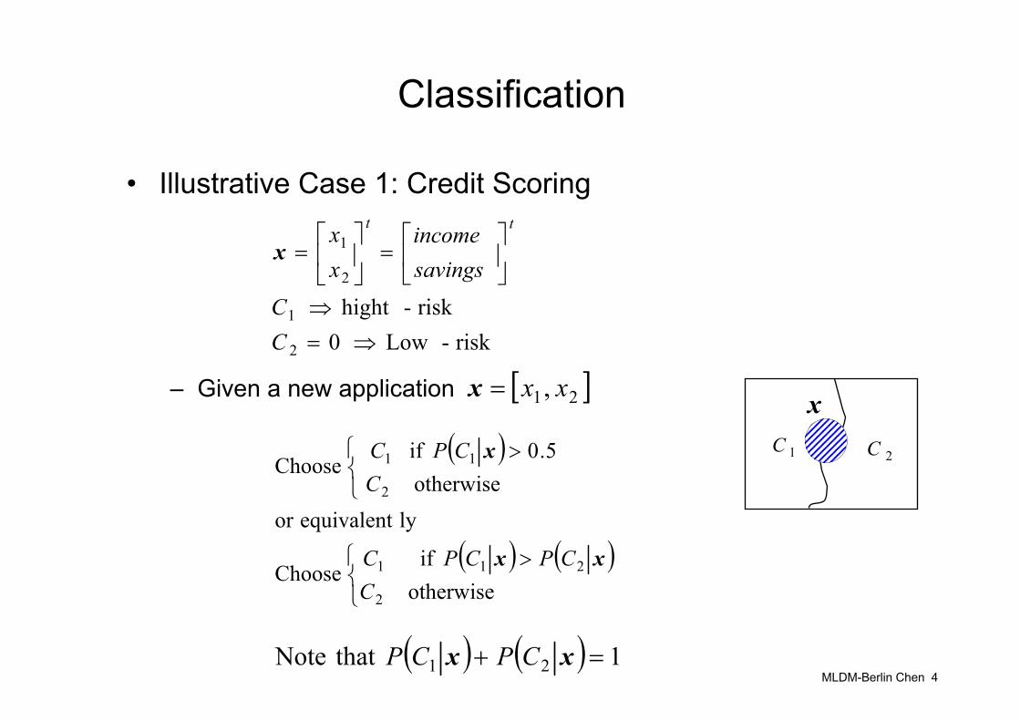
Classification
• Illustrative Case 1: Credit Scoring
– Given a new application
risk-Low 0risk-hight
2
1
2
1
⇒=⇒
⎥⎦
⎤⎢⎣
⎡=⎥
⎦
⎤⎢⎣
⎡=
CC
savingsincome
xx tt
x
[ ]21, xx=x
( )
( ) ( )⎩⎨⎧ >
⎩⎨⎧ >
otherwise if
Choose
lyequivalentor otherwise
5.0 if Choose
2
211
2
11
CCPCPC
CCPC
xx
x
( ) ( ) 1 that Note 21 =+ xx CPCP
1C 2C
x

MLDM-Berlin Chen 5
Classification (cont.)
• Bayes’ Classifier– We can use the probability theory to make inference from data
– : observed data (variable)– : class hypothesis– : prior probability of – : prior probability of – : probability of given
( ) ( ) ( )( )x
xx
PCPCP
CP =
xC
xC
( )xP( )CP
x C( )CP x
MLDM-Berlin Chen 6
Classification (cont.)
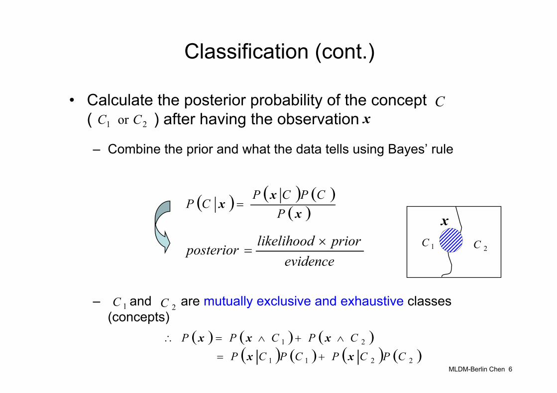
• Calculate the posterior probability of the concept ( ) after having the observation
– Combine the prior and what the data tells using Bayes’ rule
– and are mutually exclusive and exhaustive classes (concepts)
Cx
evidencepriorlikelihoodposterior ×
=
( ) ( ) ( )( )x
xx
PCPCP
CP =
1C
21 or CC
( ) ( ) ( )( ) ( ) ( ) ( )2211
21
CPCPCPCPCPCPPxx
xxx+=
∧+∧=∴
1C 2C
x
2C
MLDM-Berlin Chen 7
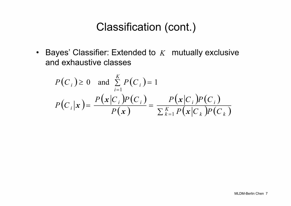
Classification (cont.)
• Bayes’ Classifier: Extended to mutually exclusive and exhaustive classes
K
( ) ( )
( ) ( ) ( )( )
( ) ( )( ) ( )∑
==
=∑≥
=
=
Kk kk
iiiii
K
iii
CPCPCPCP
PCPCP
CP
CPCP
1
11 and 0
xx
xx
x
MLDM-Berlin Chen 8
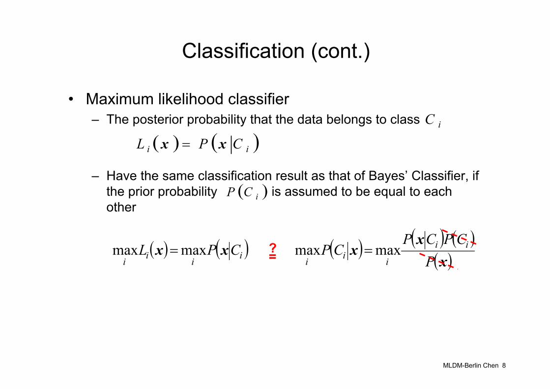
Classification (cont.)
• Maximum likelihood classifier– The posterior probability that the data belongs to class
– Have the same classification result as that of Bayes’ Classifier, if the prior probability is assumed to be equal to each other
( ) ( )ii CPL xx =iC
( )iCP
( ) ( ) ( ) ( ) ( )( )x
xxxx
PCPCP
CPCPL ii
iiiiiiimaxmax maxmax == ?=
MLDM-Berlin Chen 9
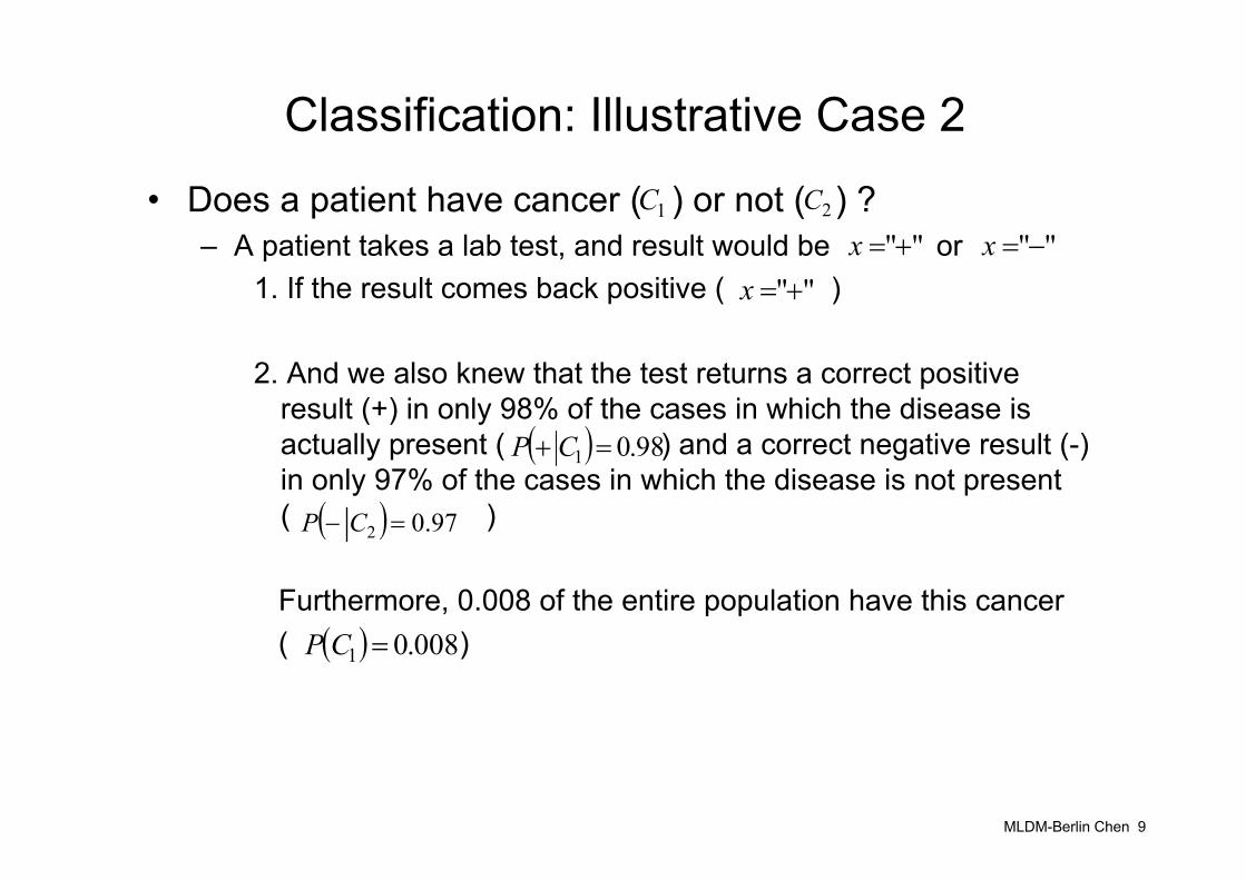
Classification: Illustrative Case 2
• Does a patient have cancer ( ) or not ( ) ? – A patient takes a lab test, and result would be or
1. If the result comes back positive ( )
2. And we also knew that the test returns a correct positive result (+) in only 98% of the cases in which the disease is actually present ( ) and a correct negative result (-) in only 97% of the cases in which the disease is not present( )
Furthermore, 0.008 of the entire population have this cancer( )
1C""−=x
2C
( ) 008.01 =CP
( ) 98.01 =+ CP
""+=x
( ) 97.02 =− CP
""+=x
MLDM-Berlin Chen 10
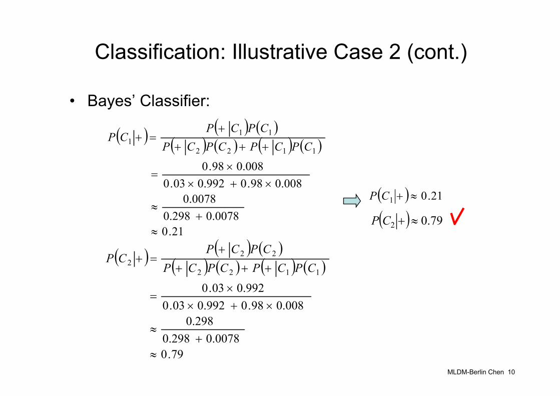
Classification: Illustrative Case 2 (cont.)
• Bayes’ Classifier:
( ) ( ) ( )( ) ( ) ( ) ( )
21.0 0.0078 0.298
0.0078
0.00898.00.99203.0 0.00898.0
1122
111
≈+
≈
×+××
=
+++
+=+
CPCPCPCPCPCP
CP
( ) 21.01 ≈+CP
( ) 79.02 ≈+CP
( ) ( ) ( )( ) ( ) ( ) ( )
79.0 0.0078 0.298
0.298
0.00898.00.99203.0 0.99203.0
1122
222
≈+
≈
×+××
=
+++
+=+
CPCPCPCPCPCP
CP
MLDM-Berlin Chen 11
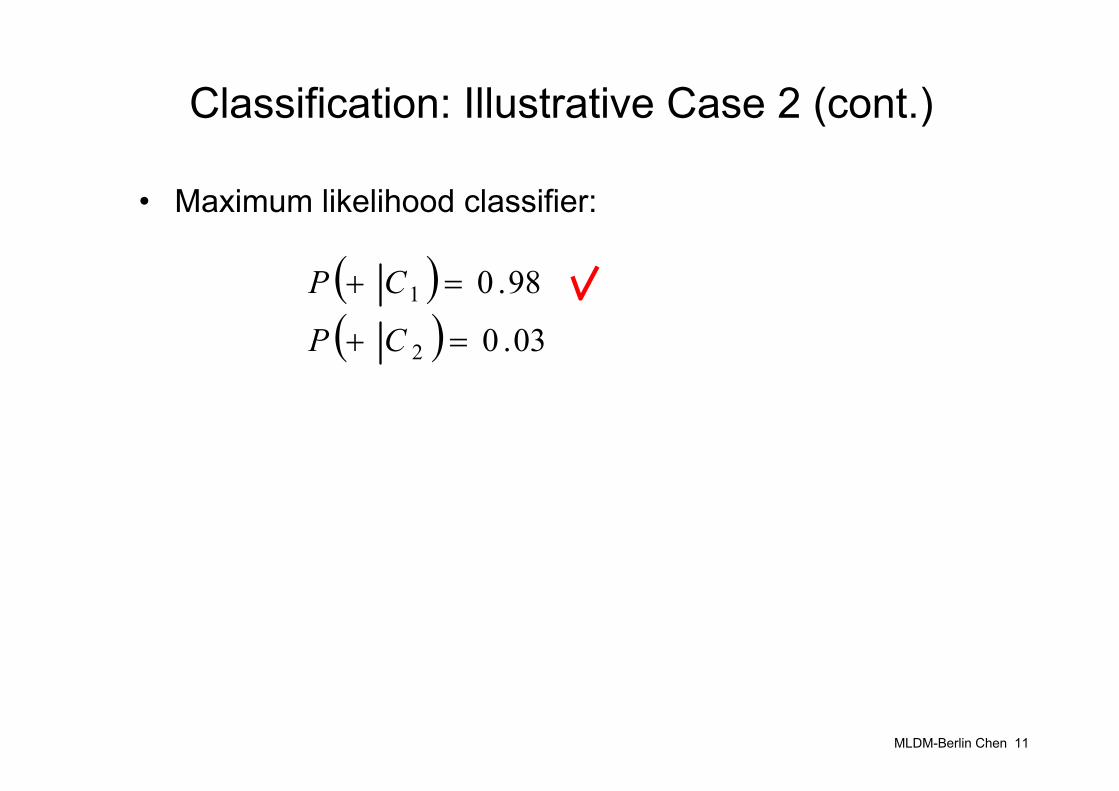
Classification: Illustrative Case 2 (cont.)
• Maximum likelihood classifier:
( )( ) 03.0
98.0
2
1
=+
=+
CP
CP
MLDM-Berlin Chen 12
Losses and Risks
• Decisions are not always prefect– E.g., “Loan Application”
• The loss for a high-risk applicant erroneously accepted (false acceptance) may be different from that for an erroneously rejected low-risk applicant (false rejection)
– Much critical for other cases such as medical diagnosis or earthquake prediction
MLDM-Berlin Chen 13
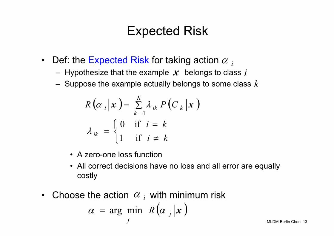
Expected Risk
• Def: the Expected Risk for taking action – Hypothesize that the example belongs to class– Suppose the example actually belongs to some class
• A zero-one loss function• All correct decisions have no loss and all error are equally
costly
• Choose the action with minimum risk
iαx
( ) ( )∑==
K
kkiki CPR
1xx λα
ik
⎩⎨⎧
≠=
=kiki
ik if 1 if 0
λ
iα( )xj
jR αα minarg=
MLDM-Berlin Chen 14
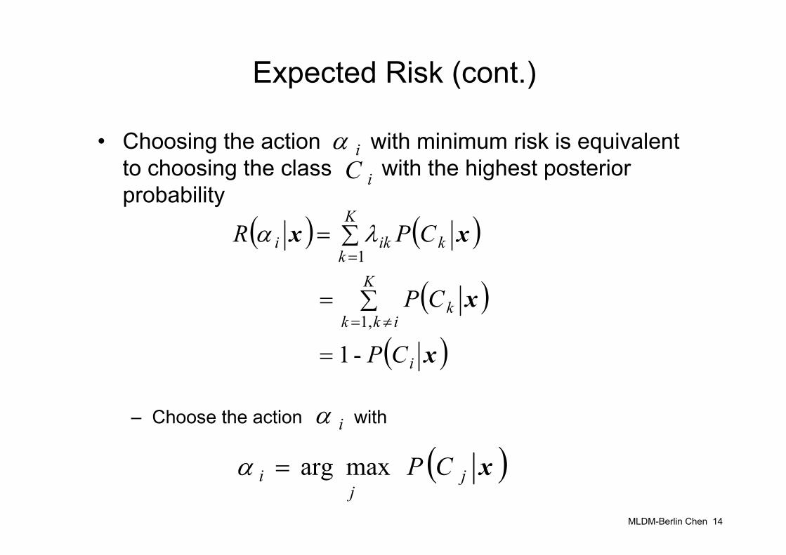
Expected Risk (cont.)
• Choosing the action with minimum risk is equivalent to choosing the class with the highest posterior probability
– Choose the action with
iαiC
( ) ( )
( )( )x
x
xx
i
K
ikkk
K
kkiki
CP
CP
CPR
-1
,1
1
=
∑=
∑=
≠=
=λα
iα
( )xjj
i CPmaxarg=α
MLDM-Berlin Chen 15
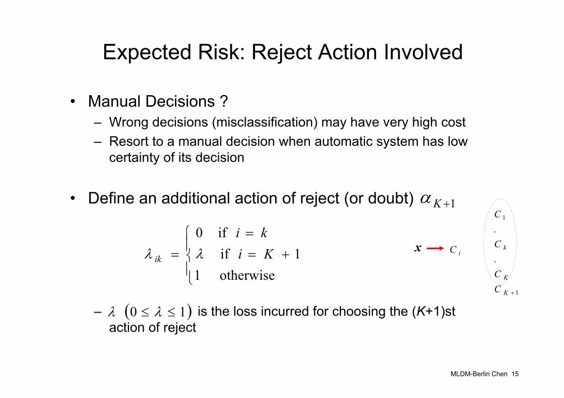
Expected Risk: Reject Action Involved
• Manual Decisions ?– Wrong decisions (misclassification) may have very high cost– Resort to a manual decision when automatic system has low
certainty of its decision
• Define an additional action of reject (or doubt)
– is the loss incurred for choosing the (K+1)st action of reject
⎪⎩
⎪⎨
⎧+=
==
otherwise 11 if
if 0Kiki
ik λλ
1+Kα
( )10 ≤≤ λλ
x
1
1
.
.
+K
K
k
CC
C
C
iC
MLDM-Berlin Chen 16
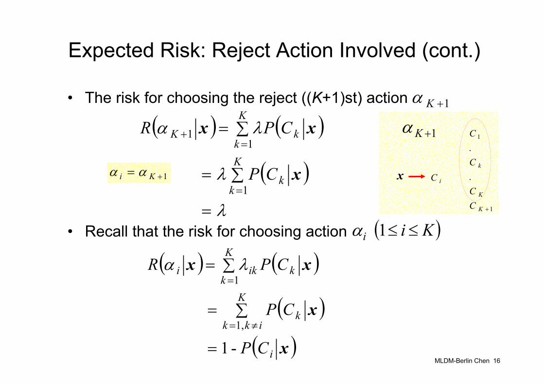
Expected Risk: Reject Action Involved (cont.)
• The risk for choosing the reject ((K+1)st) action
• Recall that the risk for choosing action
( ) ( )
( )λ
λ
λα
=
∑=
∑=
=
=+
1
11
K
kk
K
kkK
CP
CPR
x
xx
( )Kii ≤≤1 α
1+Kα
( ) ( )
( )( )x
x
xx
i
K
ikkk
K
kkiki
CP
CP
CPR
-1
,1
1
=
∑=
∑=
≠=
=λα
1+Kα
x
1
1
.
.
+K
K
k
CC
C
C
iC1+= Ki αα
MLDM-Berlin Chen 17
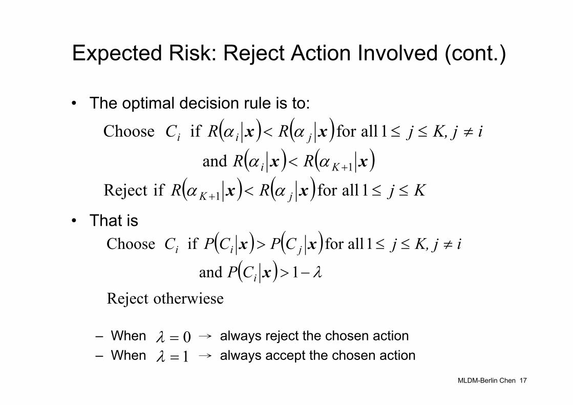
Expected Risk: Reject Action Involved (cont.)
• The optimal decision rule is to:
• That is
– When → always reject the chosen action– When → always accept the chosen action
( ) ( )( ) ( )
( ) ( ) KjRR
RR
iK, jjRRC
jK
Ki
jii
≤≤<
<
≠≤≤<
+
+
1 allfor ifReject
and
1 allfor if Choose
1
1
xx
xx
xx
αα
αα
αα
( ) ( )( )
otherwieseReject 1 and
1 allfor if Choose
λ−>
≠≤≤>
x
xx
i
jii
CP
iK, jjCPCPC
0=λ1=λ
MLDM-Berlin Chen 18
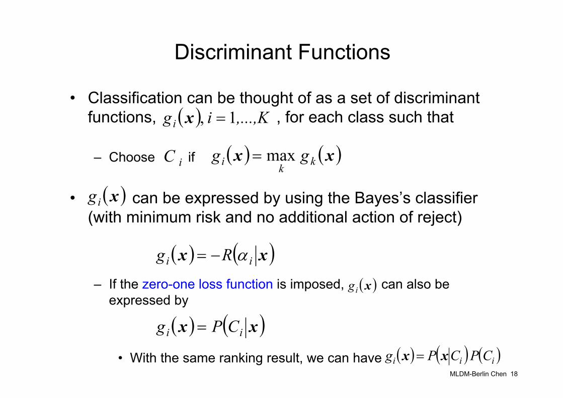
Discriminant Functions
• Classification can be thought of as a set of discriminantfunctions, , for each class such that
– Choose if
• can be expressed by using the Bayes’s classifier (with minimum risk and no additional action of reject)
– If the zero-one loss function is imposed, can also be expressed by
• With the same ranking result, we can have
( ) ,...,Kigi 1 , =x
iC ( ) ( )xx kki gg max=
( )xig
( ) ( ) xx ii Rg α−=
( ) ( ) xx ii CPg =
( ) ( ) ( ) iii CPCPg xx =
( )xig
MLDM-Berlin Chen 19
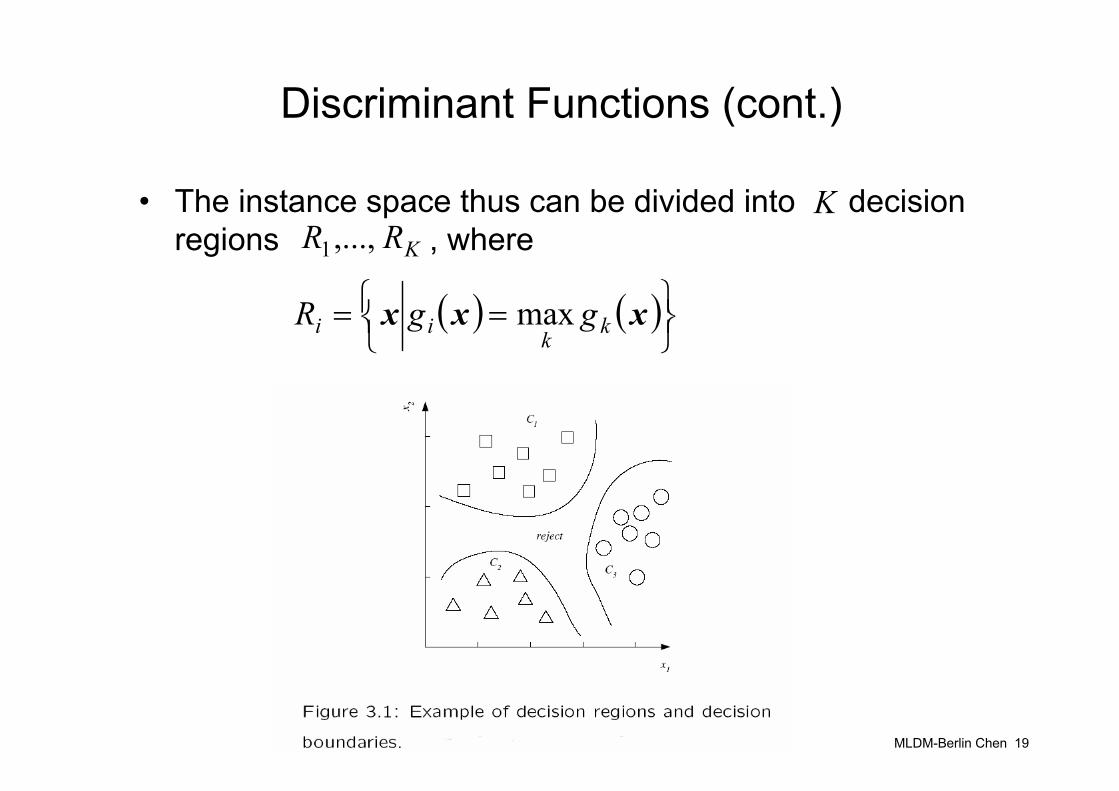
Discriminant Functions (cont.)
• The instance space thus can be divided into decision regions , where
KKRR ,...,1
( ) ( )⎭⎬⎫
⎩⎨⎧ == xxx kkii ggR max
MLDM-Berlin Chen 20
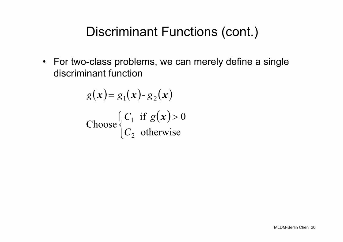
Discriminant Functions (cont.)
• For two-class problems, we can merely define a single discriminant function
( ) ( ) ( )xxx 21 - ggg =
( )⎩⎨⎧ >
otherwise 0 if
Choose2
1
Cg C x

MLDM-Berlin Chen 21
Choosing Hypotheses* : MAP Criterion
• In machine learning, we are interested in finding the best (most probable) hypothesis (classifier) hc from some hypothesis space H, given the observed training data set
– A Maximum a Posteriori (MAP) hypothesis
( ){ }ntcrrxX ittt
c i,,2,1 ,, L===
( )( ) ( )
( )( ) ( )
iiiic
i
iii
ic
iiic
cccHh
c
ccc
Hh
ccHhMAP
hPhP
P
hPhP
hPh
X
X
X
X
∈
∈
∈
=
=
=
maxarg
maxarg
maxarg
MAPh
MLDM-Berlin Chen 22
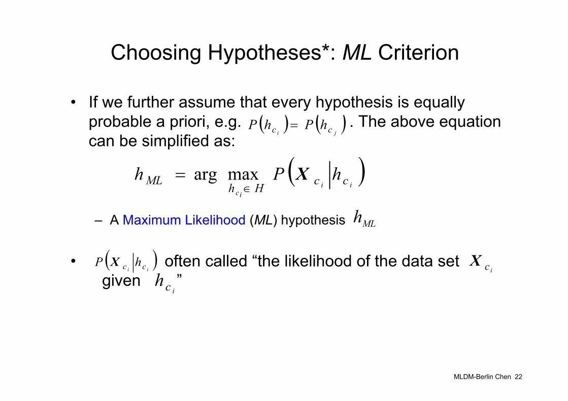
Choosing Hypotheses*: ML Criterion
• If we further assume that every hypothesis is equally probable a priori, e.g. . The above equation can be simplified as:
– A Maximum Likelihood (ML) hypothesis
• often called “the likelihood of the data setgiven ”
( )ii
icccHhML hPh X
∈= maxarg
( ) ( )ji cc hPhP =
MLh
ichicX( )
ii cc hP X
MLDM-Berlin Chen 23
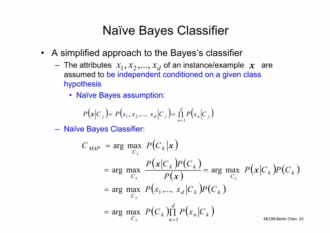
Naïve Bayes Classifier
• A simplified approach to the Bayes’s classifier– The attributes of an instance/example are
assumed to be independent conditioned on a given class hypothesis
• Naïve Bayes assumption:
– Naïve Bayes Classifier:
dxxx ,...,, 21 x
( ) ( ) ( )∏===
d
njnjdj CxPCxxxPCP
121 ,...,,x
( )( ) ( )
( ) ( ) ( )
( ) ( )
( ) ( )∏=
=
==
=
=
d
nknkC
kkdC
kkC
kk
C
kCMAP
CxPCP
CPCxxP
CPCPP
CPCP
CPC
k
k
kk
k
1
1
maxarg
,...,maxarg
maxargmaxarg
maxarg
xx
x
x

MLDM-Berlin Chen 24
Naïve Bayes Classifier (cont.)
• Illustrative case 1– Given a data set with 3-dimensional Boolean
examples , train a naïve Bayes classifier to predict the classification
– What is the predicted probability ? – What is the predicted probability ?
( )CBA xxx ,,=x
FTFF
FTTF
FFFT
TFFT
TTFF
TFTF
Classification DAttribute C
Attribute B
Attribute A
( ) ( )
( ) ( )( ) ( )( ) ( )
( ) ( )( ) ( )( ) ( ) 3/1 ,3/2
3/2 ,3/1
3/2 ,3/1
3/2 ,3/1
3/2 ,3/1
3/2 ,3/1
2/1 ,2/1
======
======
======
======
======
======
====
FDFBPFDTCP
FDFBPFDTBP
FDFAPFDTAP
TDFBPTDTCP
TDFBPTDTBP
TDFAPTDTAP
FDPTDP
( )TCFBTATDP ==== ,,
( )TBTDP ==
( )CBA xxx ,,=x
MLDM-Berlin Chen 25
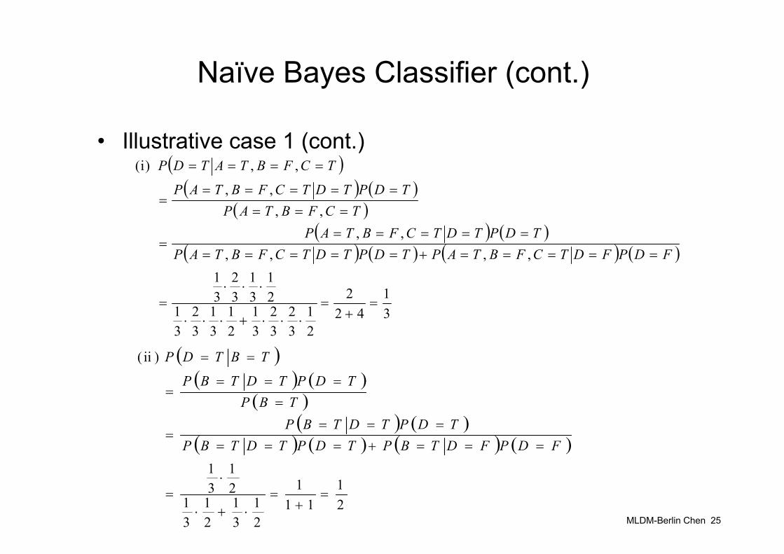
Naïve Bayes Classifier (cont.)
• Illustrative case 1 (cont.)( )( ) ( )
( )( ) ( )
( ) ( ) ( ) ( )
31
422
21
32
32
31
21
31
32
31
21
31
32
31
,,,,,,
,,,,
,, )i(
=+
=⋅⋅⋅+⋅⋅⋅
⋅⋅⋅=
=====+==========
=
========
=
====
FDPFDTCFBTAPTDPTDTCFBTAPTDPTDTCFBTAP
TCFBTAPTDPTDTCFBTAP
TCFBTATDP
( )( ) ( )
( )( ) ( )
( ) ( ) ( ) ( )
21
111
21
31
21
31
21
31
)ii(
=+
=⋅+⋅
⋅=
===+======
=
====
=
==
FDPFDTBPTDPTDTBPTDPTDTBP
TBPTDPTDTBP
TBTDP
MLDM-Berlin Chen 26
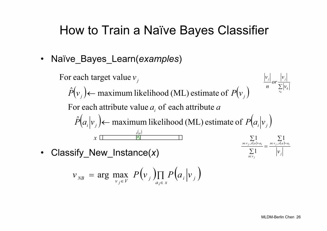
How to Train a Naïve Bayes Classifier
• Naïve_Bayes_Learn(examples)
• Classify_New_Instance(x)
( ) ( )
( ) ( )jiji
i
jj
j
vaPvaP
aavPvP
v
of estimate (ML) likelihood maximumˆ
attributeeach of valueattributeeach For of estimate (ML) likelihood maximumˆ
t valueeach targeFor
←
←
( ) ( )∏=∈∈ xa
jijVvNBij
vaPvPv maxarg
∑kv
k
jj
vv
ornv
( ) ( )
j
aaxvx
vx
aaxvx
vij
j
ij
∑=
∑
∑=∈
∈
=∈ ,,1
1
1( )axiax
MLDM-Berlin Chen 27
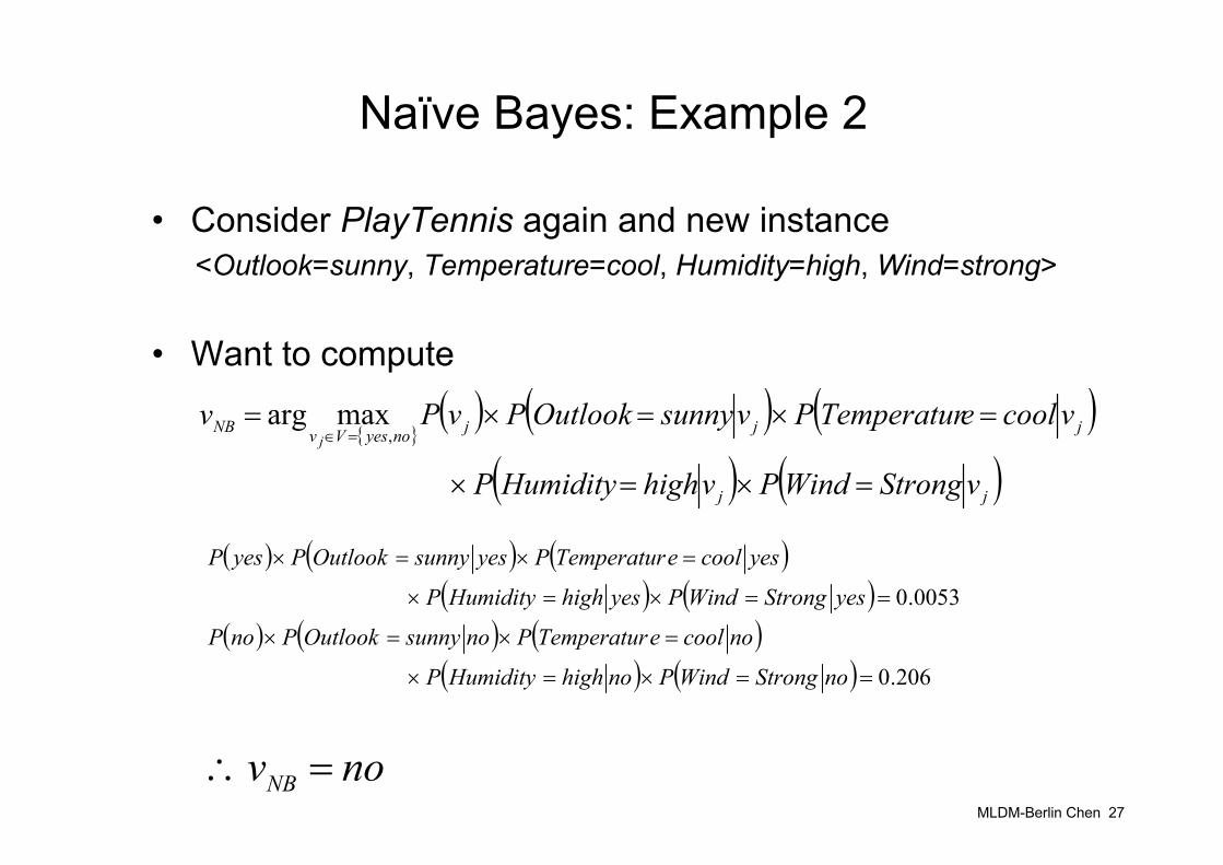
Naïve Bayes: Example 2
• Consider PlayTennis again and new instance<Outlook=sunny, Temperature=cool, Humidity=high, Wind=strong>
• Want to compute
( ) ( ) ( )( ) ( )
( ) ( ) ( )( ) ( ) 206.0
0053.0
==×=×
=×=×
==×=×
=×=×
noStrongWindPnohighHumidityP
nocooleTemperaturPnosunnyOutlookPnoP
yesStrongWindPyeshighHumidityP
yescooleTemperaturPyessunnyOutlookPyesP
{ }( ) ( ) ( )
( ) ( )jj
jjjnoyesVvNB
vStrongWindPvhighHumidityP
vcooleTemperaturPvsunnyOutlookPvPvj
=×=×
=×=×==∈
maxarg,
novNB =∴
MLDM-Berlin Chen 28
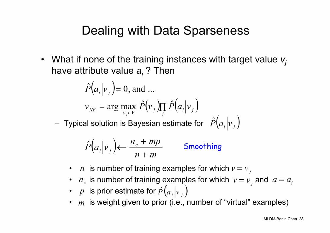
Dealing with Data Sparseness
• What if none of the training instances with target value vjhave attribute value ai ? Then
– Typical solution is Bayesian estimate for
• is number of training examples for which• is number of training examples for which and • is prior estimate for • is weight given to prior (i.e., number of “virtual” examples)
( )( ) ( )∏=
=
∈ ijijVvNB
ji
vaPvPv
vaP
j
ˆˆmaxarg
... and ,0ˆ
( )ji vaP̂
ncn
pm
jvv =jvv = iaa =
( )ji vaP̂
( )mnmpnvaP c
ji ++
←ˆ Smoothing
MLDM-Berlin Chen 29
Example: Learning to Classify Text
• For instance,– Learn which news articles are of interest– Learn to classify web pages by topic
• Naïve Bayes is among the most effective algorithms
• What attributes shall we use to represent text documents– The word occurs in each document position
MLDM-Berlin Chen 30
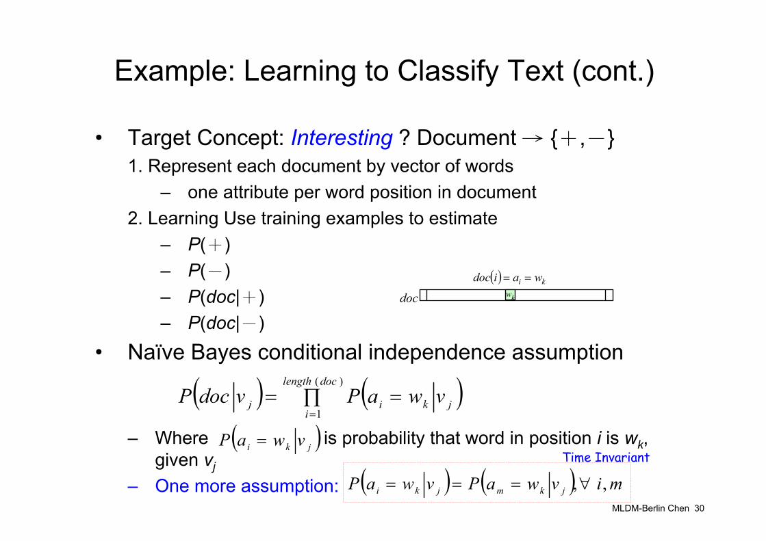
Example: Learning to Classify Text (cont.)
• Target Concept: Interesting ? Document → {+,-}1. Represent each document by vector of words
– one attribute per word position in document2. Learning Use training examples to estimate
– P(+)– P(-)– P(doc|+)– P(doc|-)
• Naïve Bayes conditional independence assumption
– Where is probability that word in position i is wk, given vj
– One more assumption:
( ) ( )∏ ===
)(
1
doclength
ijkij vwaPvdocP
( )jki vwaP =
( ) ( ) mivwaPvwaP jkmjki , ,∀===
Time Invariant
( ) ki waidoc ==
kwdoc

MLDM-Berlin Chen 31
Example: Learning to Classify Text (cont.)
• Learn_Naïve_Bayes_Text(Examples, V)
1. Collect all words and other tokens that occur in Examples• Vocabulary ← all distinct words and other tokens in Examples
2. Calculate the required and probability terms• ← subset of Examples for which the target value is• ←
• ← a single document created by concatenating all members of
• ← total number of words in (counting duplicate words multiple times)
• For each word in Vocabulary– ← number of times word occurs in– ←
( )jvP ( )jk vwP
jdocs jv( )jvP
Examplesdocs j
jTextjdocs
n jText
kn kwkw
( )jk vwPVocabularyn
nk
++ 1
Smoothed unigram
MLDM-Berlin Chen 32
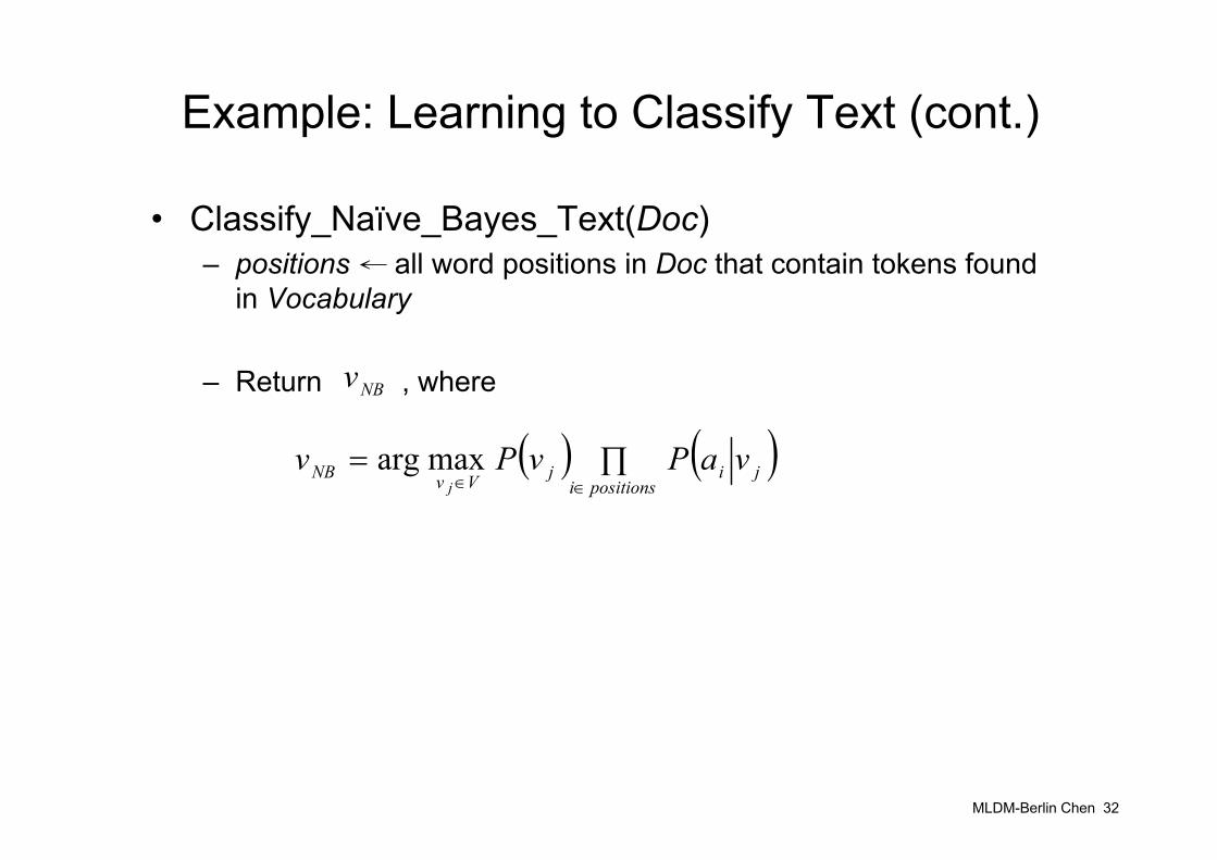
Example: Learning to Classify Text (cont.)
• Classify_Naïve_Bayes_Text(Doc)– positions ← all word positions in Doc that contain tokens found
in Vocabulary
– Return , where
( ) ( )∏=∈∈ positionsi
jijVvNB vaPvPvj
maxarg
NBv
MLDM-Berlin Chen 33
Bayesian Networks
• Premise– Naïve Bayes assumption of conditional independence too
restrictive
– But it is intractable without some such assumptions
– Bayesian networks describe conditional independence among subsets of variables
• Allows combining prior knowledge about (in)dependenciesamong variables with observed training data
• Bayesian Networks also called– Bayesian Belief Networks, Bayes Nets, Belief Networks,
Probabilistic Networks, Graphical Models etc.
MLDM-Berlin Chen 34
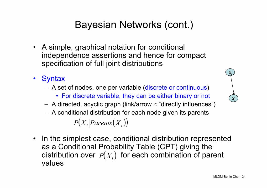
Bayesian Networks (cont.)
• A simple, graphical notation for conditional independence assertions and hence for compact specification of full joint distributions
• Syntax– A set of nodes, one per variable (discrete or continuous)
• For discrete variable, they can be either binary or not– A directed, acyclic graph (link/arrow ≈ “directly influences”)– A conditional distribution for each node given its parents
• In the simplest case, conditional distribution represented as a Conditional Probability Table (CPT) giving the distribution over for each combination of parent values
( )( )ii XParentsXP
( )iXP
xi
xj
MLDM-Berlin Chen 35
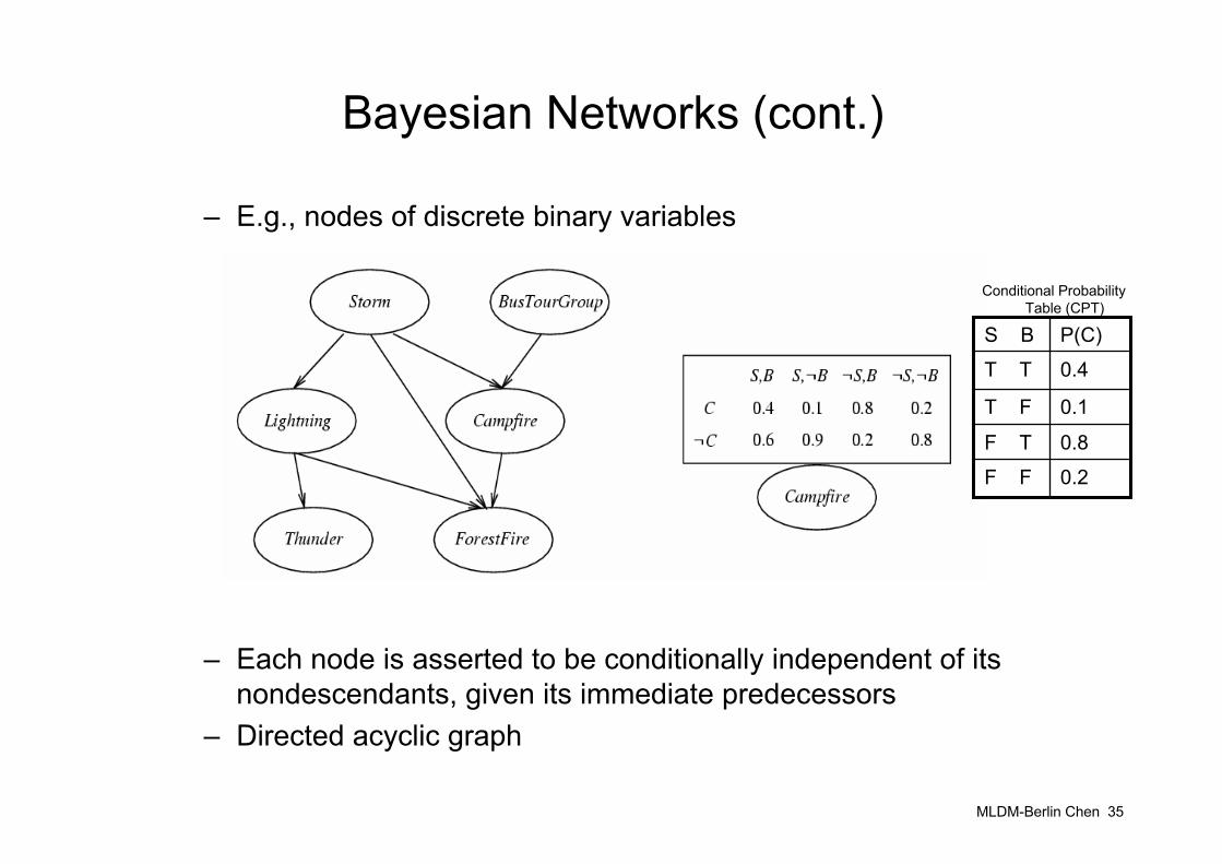
Bayesian Networks (cont.)
– E.g., nodes of discrete binary variables
– Each node is asserted to be conditionally independent of its nondescendants, given its immediate predecessors
– Directed acyclic graph
0.2F F
0.8F T
0.1T F
0.4T T
P(C)S B
Conditional ProbabilityTable (CPT)
MLDM-Berlin Chen 36
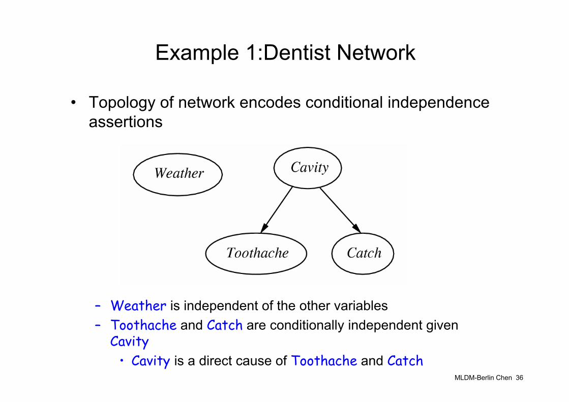
Example 1:Dentist Network
• Topology of network encodes conditional independence assertions
– Weather is independent of the other variables– Toothache and Catch are conditionally independent given
Cavity• Cavity is a direct cause of Toothache and Catch
MLDM-Berlin Chen 37
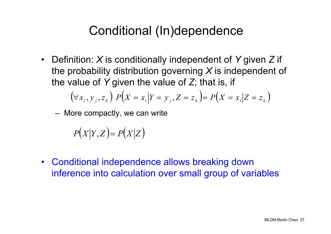
Conditional (In)dependence
• Definition: X is conditionally independent of Y given Z if the probability distribution governing X is independent of the value of Y given the value of Z; that is, if
– More compactly, we can write
• Conditional independence allows breaking down inference into calculation over small group of variables
( ) ( )ZXPZYXP =,
( ) ( ) ( )kikjikji zZxXPzZyYxXPzyx ======∀ , ,,
MLDM-Berlin Chen 38
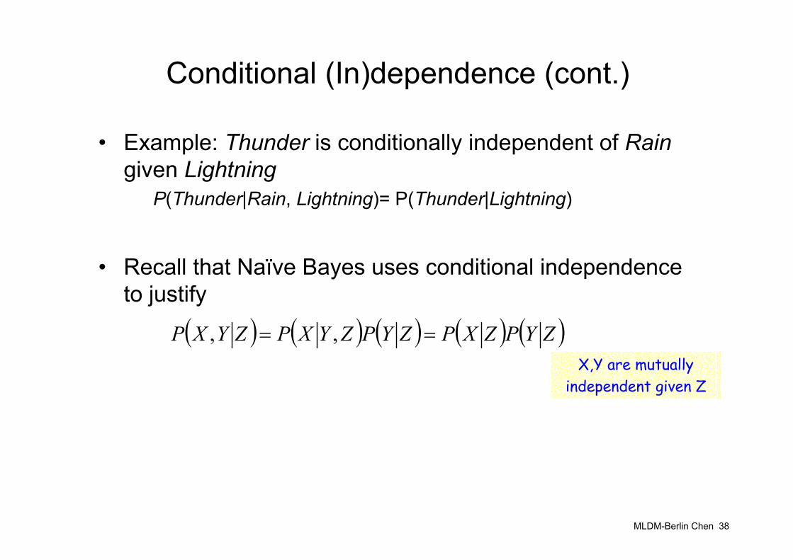
Conditional (In)dependence (cont.)
• Example: Thunder is conditionally independent of Raingiven Lightning
P(Thunder|Rain, Lightning)= P(Thunder|Lightning)
• Recall that Naïve Bayes uses conditional independence to justify
( ) ( ) ( ) ( ) ( )ZYPZXPZYPZYXPZYXP == ,,X,Y are mutually
independent given Z
MLDM-Berlin Chen 39
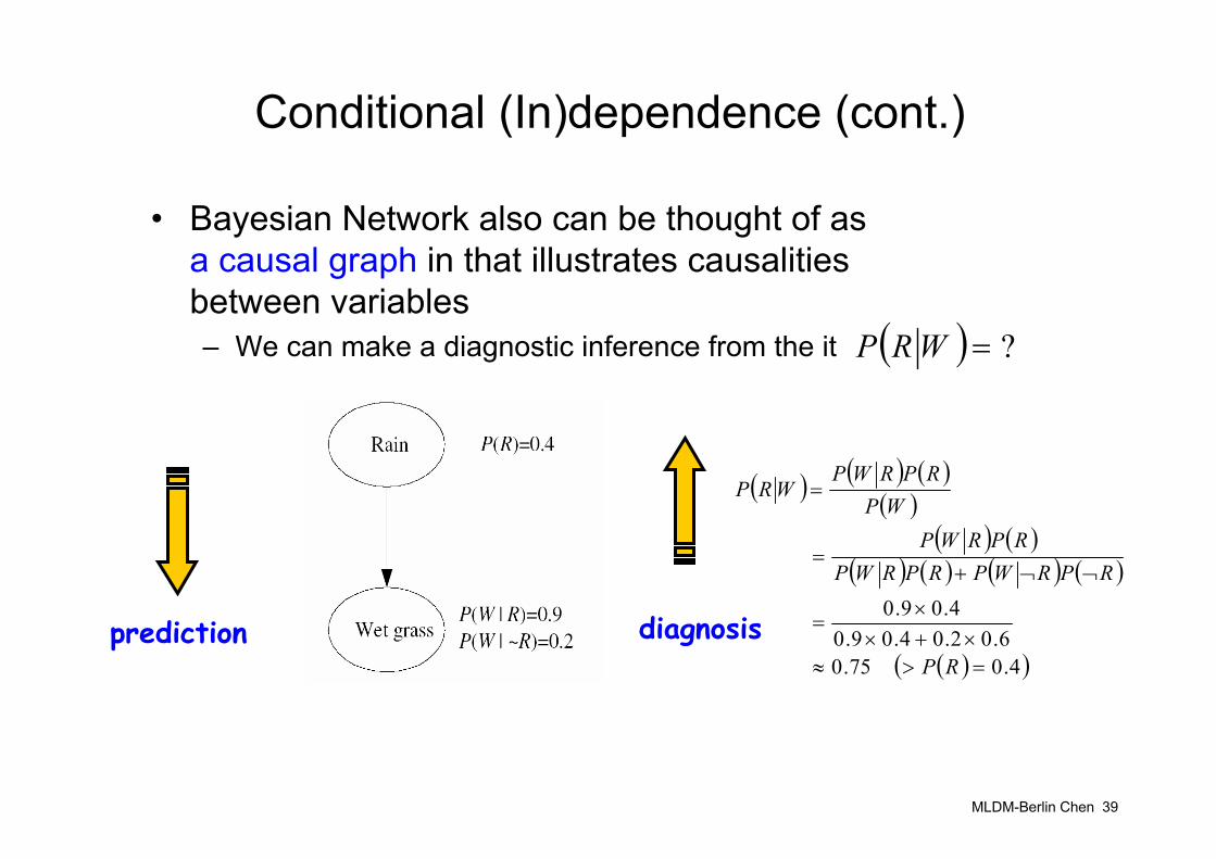
Conditional (In)dependence (cont.)
• Bayesian Network also can be thought of asa causal graph in that illustrates causalities between variables– We can make a diagnostic inference from the it ( ) ?=WRP
prediction diagnosis
( ) ( ) ( )( )
( ) ( )( ) ( ) ( ) ( )
( )( )4.0 75.0 6.02.04.09.0
4.09.0
=>≈×+×
×=
¬¬+=
=
RP
RPRWPRPRWPRPRWP
WPRPRWP
WRP

MLDM-Berlin Chen 40
Conditional (In)dependence (cont.)
• Suppose that sprinkler is included as another cause of wet grass
– Predictive inference
– Diagnostic inference (I)
( )( ) ( ) ( ) ( )( ) ( ) ( ) ( )
92.06.09.04.095.0
,,
,,
≈×+×=
¬¬+=
¬¬+=
RPSRWPRPSRWP
SRPSRWPSRPSRWP
SWP
( )( ) ( )
( )
( )( )2.0 35.052.0
2.092.0
=>≈
×≈
=
SP
WPSPSWP
WSP
( ) ( ) ( ) ( ) ( )( ) ( ) ( ) ( )( ) ( ) ( ) ( ) ( ) ( )( ) ( ) ( ) ( ) ( ) ( )
250. 0.80.60.10.80.40.90.20.60.90.20.40.95
,,
,,
,,,,
,,,,
=××+××+××+××=
¬¬¬¬+¬¬+
¬¬+=
¬¬¬¬+¬¬+
¬¬+=
SPRPSRWPSPRPSRWP
SPRPSRWPSPRPSRWP
SRPSRWPSRPSRWP
SRPSRWPSRPSRWPWP
MLDM-Berlin Chen 41
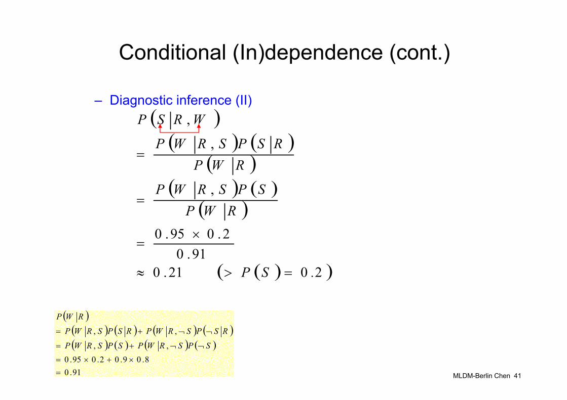
Conditional (In)dependence (cont.)
– Diagnostic inference (II)( )( ) ( )
( )( ) ( )
( )
( )( )20 21.091.0
2.095.0
,
,
,
.SP
RWPSPSRWP
RWPRSPSRWP
WRSP
=>≈
×=
=
=
( )( ) ( ) ( ) ( )( ) ( ) ( ) ( )
91.08.09.02.095.0
,,
,,
=×+×=
¬¬+=
¬¬+=
SPSRWPSPSRWP
RSPSRWPRSPSRWP
RWP
MLDM-Berlin Chen 42
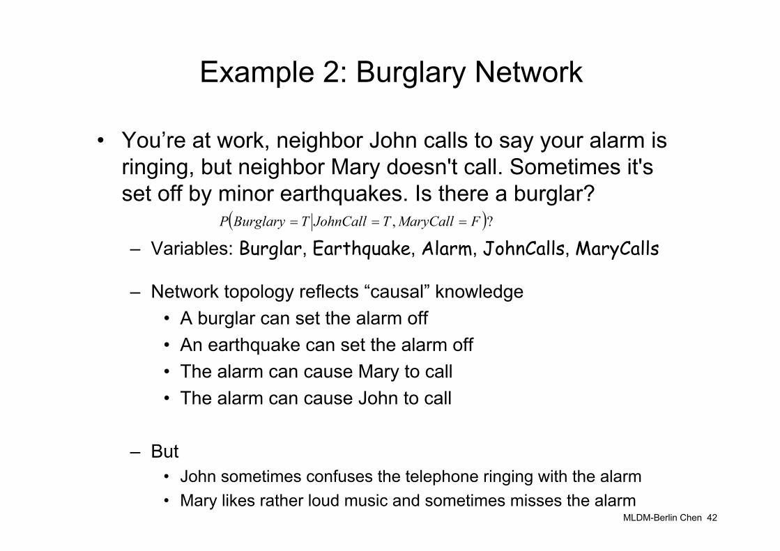
Example 2: Burglary Network
• You’re at work, neighbor John calls to say your alarm is ringing, but neighbor Mary doesn't call. Sometimes it's set off by minor earthquakes. Is there a burglar?
– Variables: Burglar, Earthquake, Alarm, JohnCalls, MaryCalls
– Network topology reflects “causal” knowledge• A burglar can set the alarm off• An earthquake can set the alarm off• The alarm can cause Mary to call• The alarm can cause John to call
– But • John sometimes confuses the telephone ringing with the alarm• Mary likes rather loud music and sometimes misses the alarm
( )?, FMaryCallTJohnCallTBurglaryP ===
MLDM-Berlin Chen 43
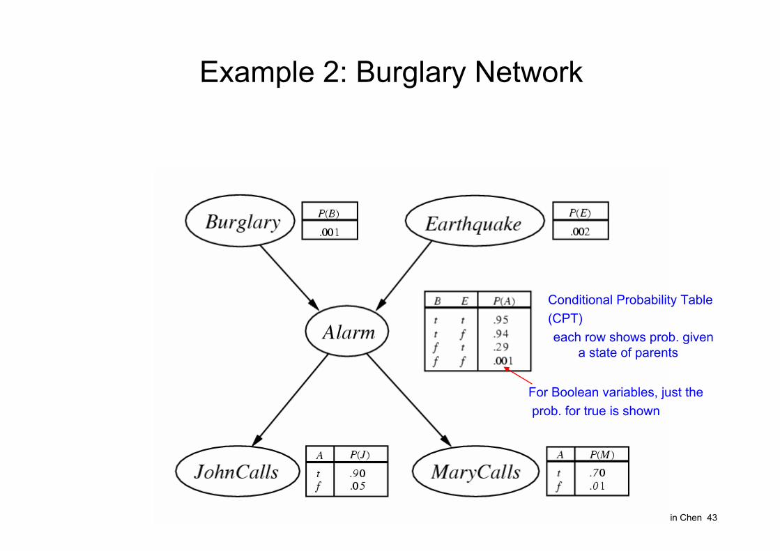
Example 2: Burglary Network
Conditional Probability Table(CPT)
For Boolean variables, just theprob. for true is shown
each row shows prob. givena state of parents
MLDM-Berlin Chen 44
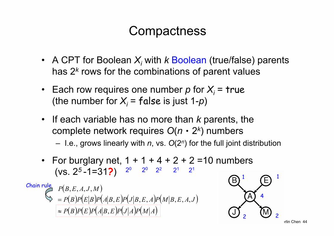
Compactness
• A CPT for Boolean Xi with k Boolean (true/false) parents has 2k rows for the combinations of parent values
• Each row requires one number p for Xi = true(the number for Xi = false is just 1-p)
• If each variable has no more than k parents, the complete network requires O(n‧2k) numbers– I.e., grows linearly with n, vs. O(2n) for the full joint distribution
• For burglary net, 1 + 1 + 4 + 2 + 2 =10 numbers(vs. 25 -1=31?)
1 1
4
2 2
( )( ) ( ) ( ) ( ) ( )( ) ( ) ( ) ( ) ( )AMPAJPEBAPEPBP
JAEBMPAEBJPEBAPBEPBPMJAEBP
,
,,,,,,,,,,
≈
=
Chain rule
20 20 22 21 21
MLDM-Berlin Chen 45
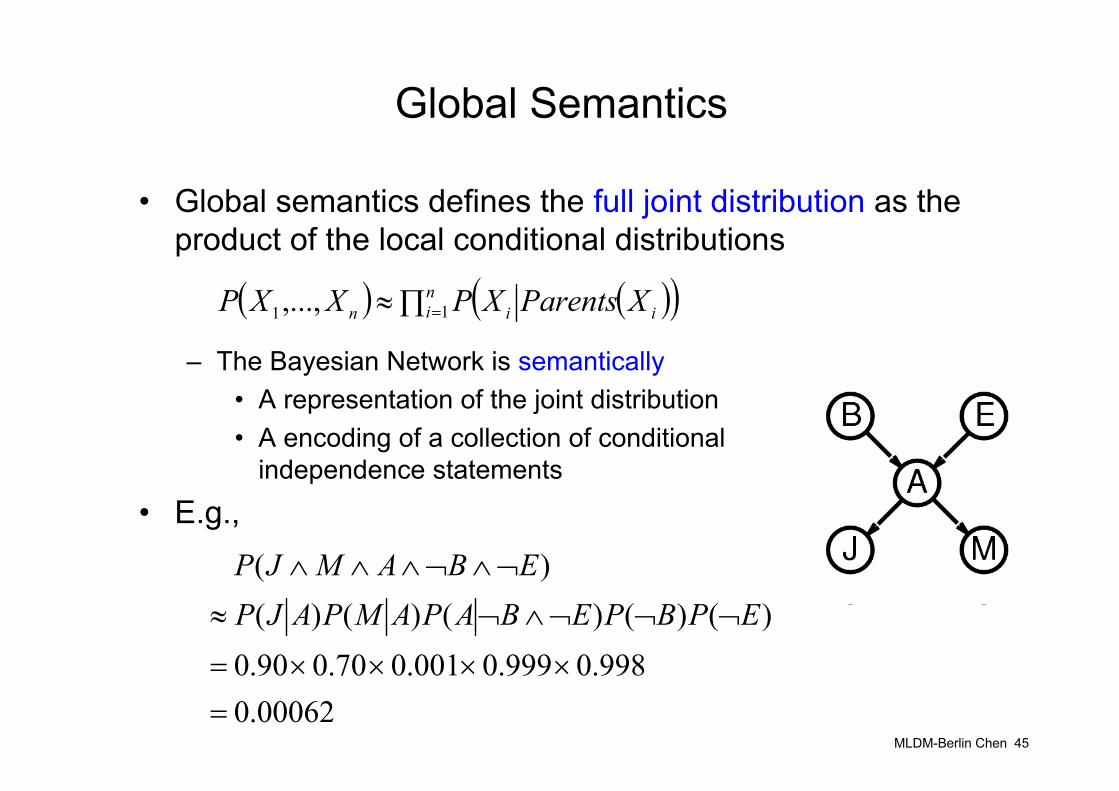
Global Semantics
• Global semantics defines the full joint distribution as the product of the local conditional distributions
– The Bayesian Network is semantically• A representation of the joint distribution• A encoding of a collection of conditional
independence statements
• E.g.,
( ) ( )( )∏≈ =ni iin XParentsXPXXP 11,...,
00062.0998.0999.0001.070.090.0
)()()()()()(
=××××=
¬¬¬∧¬≈
¬∧¬∧∧∧
EPBPEBAPAMPAJPEBAMJP
MLDM-Berlin Chen 46
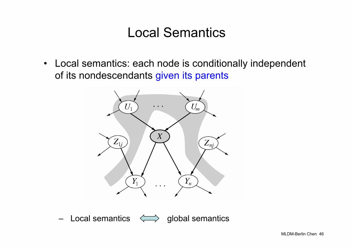
Local Semantics
• Local semantics: each node is conditionally independent of its nondescendants given its parents
– Local semantics global semantics
MLDM-Berlin Chen 47
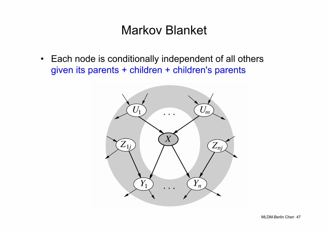
Markov Blanket
• Each node is conditionally independent of all others given its parents + children + children's parents
MLDM-Berlin Chen 48
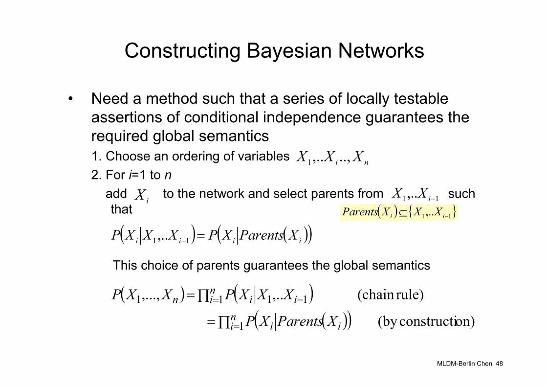
Constructing Bayesian Networks
• Need a method such that a series of locally testable assertions of conditional independence guarantees the required global semantics1. Choose an ordering of variables2. For i=1 to n
add to the network and select parents from such that
This choice of parents guarantees the global semantics
ni XXX ..,,..1
iX 11,.. −iXX
( ) ( )( )iiii XParentsXPXXXP =−11,..
( ) ( )( )( )∏=
∏=
=
= −
ni ii
ni iin
XParentsXP
XXXPXXP
1
1 111
on)constructi(by
rule)(chain ,..,...,
( ) { }11,.. −⊆ ii XXXParents
MLDM-Berlin Chen 49
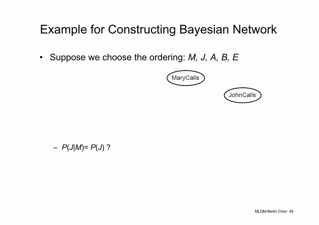
Example for Constructing Bayesian Network
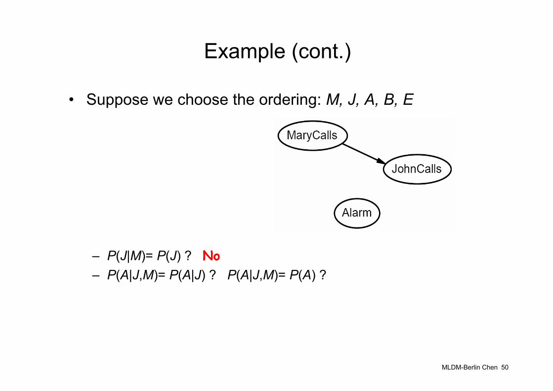
• Suppose we choose the ordering: M, J, A, B, E
– P(J|M)= P(J) ?
MLDM-Berlin Chen 50
Example (cont.)
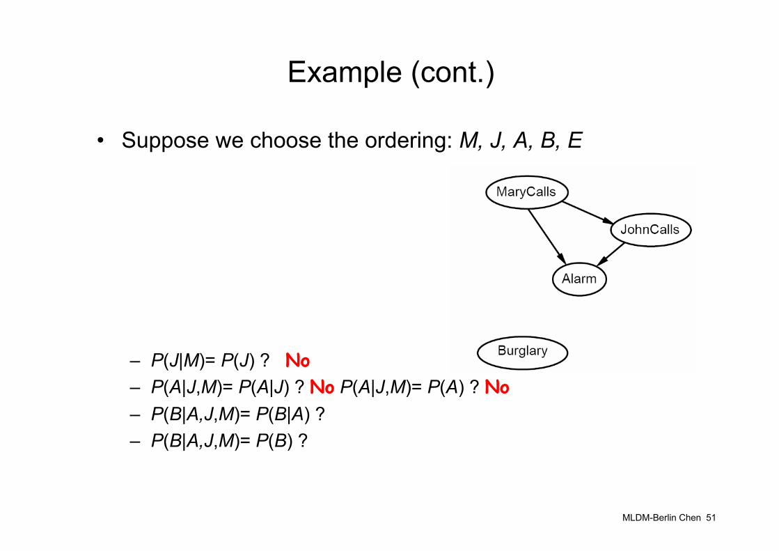
• Suppose we choose the ordering: M, J, A, B, E
– P(J|M)= P(J) ? No– P(A|J,M)= P(A|J) ? P(A|J,M)= P(A) ?
MLDM-Berlin Chen 51
Example (cont.)
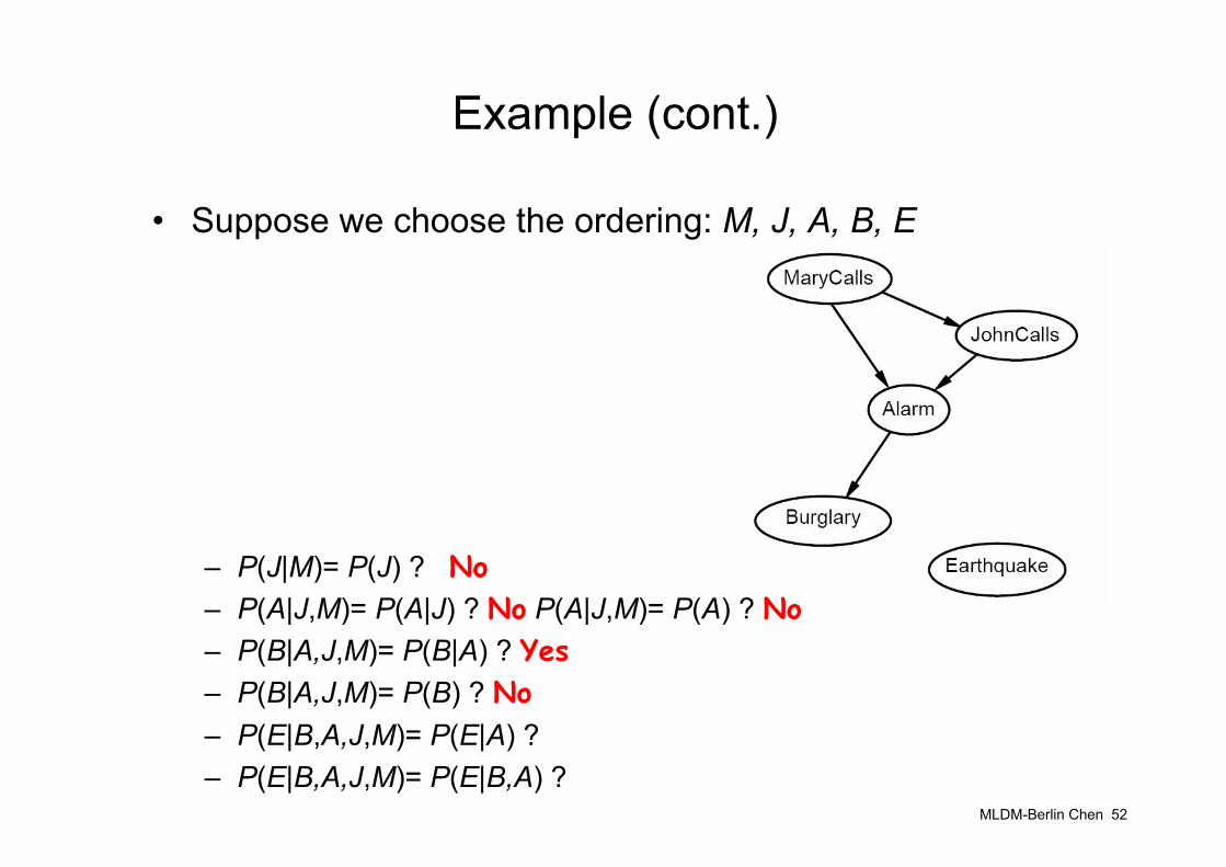
• Suppose we choose the ordering: M, J, A, B, E
– P(J|M)= P(J) ? No– P(A|J,M)= P(A|J) ? No P(A|J,M)= P(A) ? No– P(B|A,J,M)= P(B|A) ?– P(B|A,J,M)= P(B) ?
MLDM-Berlin Chen 52
Example (cont.)
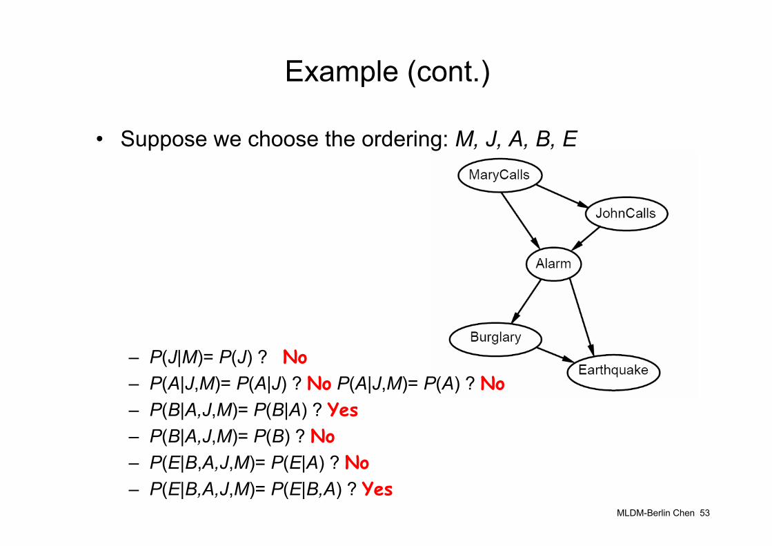
• Suppose we choose the ordering: M, J, A, B, E
– P(J|M)= P(J) ? No– P(A|J,M)= P(A|J) ? No P(A|J,M)= P(A) ? No– P(B|A,J,M)= P(B|A) ? Yes– P(B|A,J,M)= P(B) ? No– P(E|B,A,J,M)= P(E|A) ? – P(E|B,A,J,M)= P(E|B,A) ?
MLDM-Berlin Chen 53
Example (cont.)
• Suppose we choose the ordering: M, J, A, B, E
– P(J|M)= P(J) ? No– P(A|J,M)= P(A|J) ? No P(A|J,M)= P(A) ? No– P(B|A,J,M)= P(B|A) ? Yes– P(B|A,J,M)= P(B) ? No– P(E|B,A,J,M)= P(E|A) ? No– P(E|B,A,J,M)= P(E|B,A) ? Yes
MLDM-Berlin Chen 54
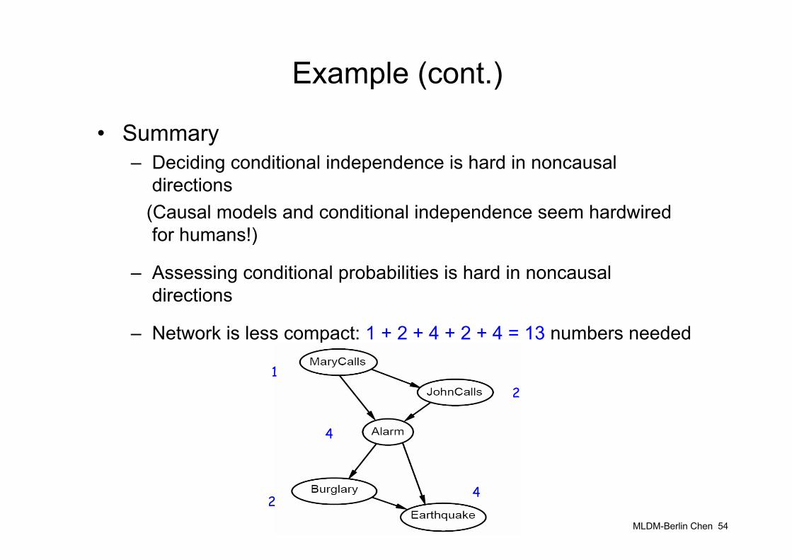
Example (cont.)
• Summary– Deciding conditional independence is hard in noncausal
directions(Causal models and conditional independence seem hardwired for humans!)
– Assessing conditional probabilities is hard in noncausaldirections
– Network is less compact: 1 + 2 + 4 + 2 + 4 = 13 numbers needed
12
4
24
MLDM-Berlin Chen 55
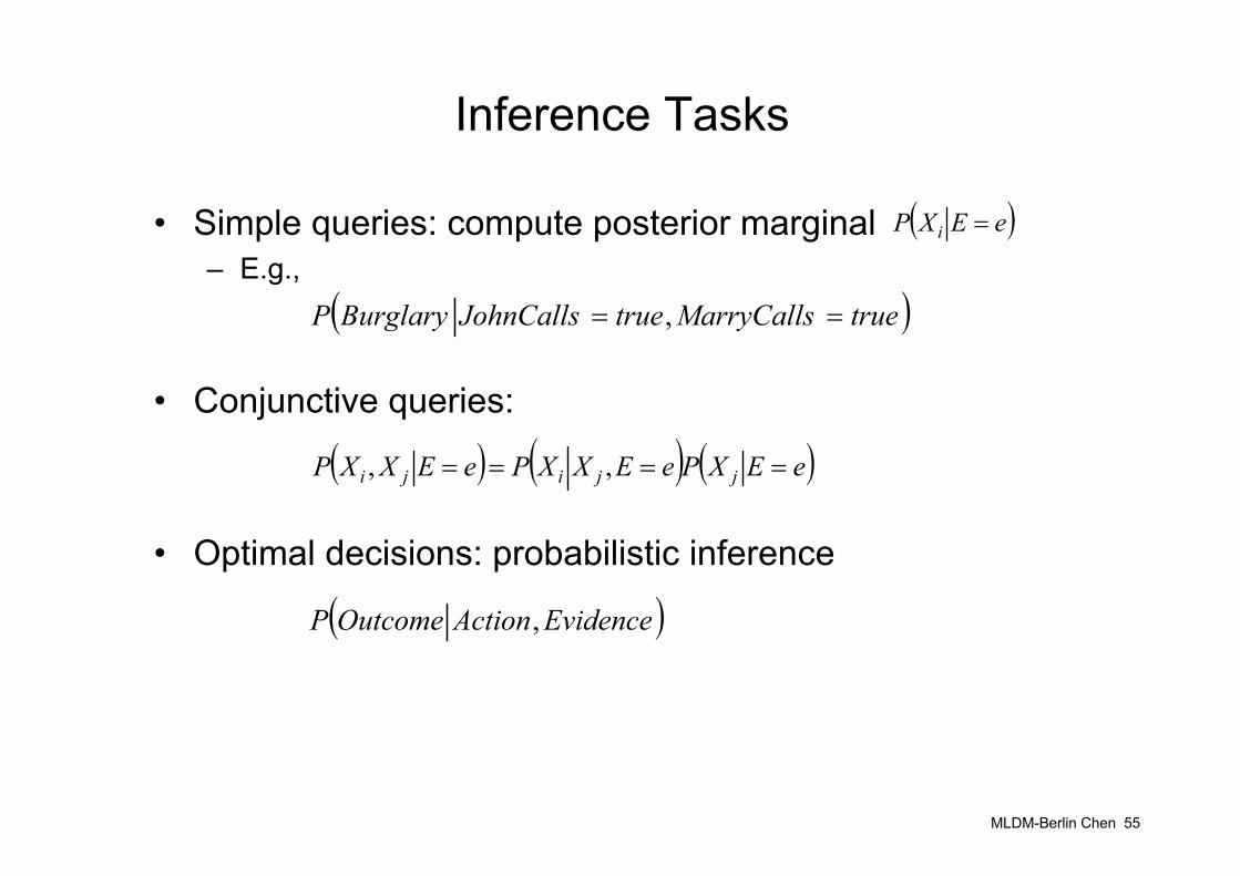
Inference Tasks
• Simple queries: compute posterior marginal– E.g.,
• Conjunctive queries:
• Optimal decisions: probabilistic inference
( )eEXP i =
( )trueMarryCallstrueJohnCallsBurglaryP == ,
( ) ( ) ( )eEXPeEXXPeEXXP jjiji ==== ,,
( )EvidenceActionOutcomeP ,
MLDM-Berlin Chen 56
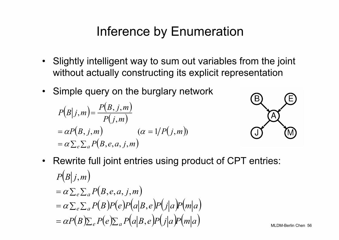
Inference by Enumeration
• Slightly intelligent way to sum out variables from the joint without actually constructing its explicit representation
• Simple query on the burglary network
• Rewrite full joint entries using product of CPT entries:( )
( )( ) ( ) ( ) ( ) ( )
( ) ( ) ( ) ( ) ( )amPajPeBaPePBP
amPajPeBaPePBPmjaeBP
mjBP
e a
e a
e a
∑ ∑=
∑ ∑=
∑ ∑=
,
,,,,,
,
α
α
α
( ) ( )( )
( ) ( )( )∑ ∑=
==
=
e a mjaeBPmjPmjBP
mjPmjBPmjBP
,,,,),1( ,,
,,,,
ααα
MLDM-Berlin Chen 57
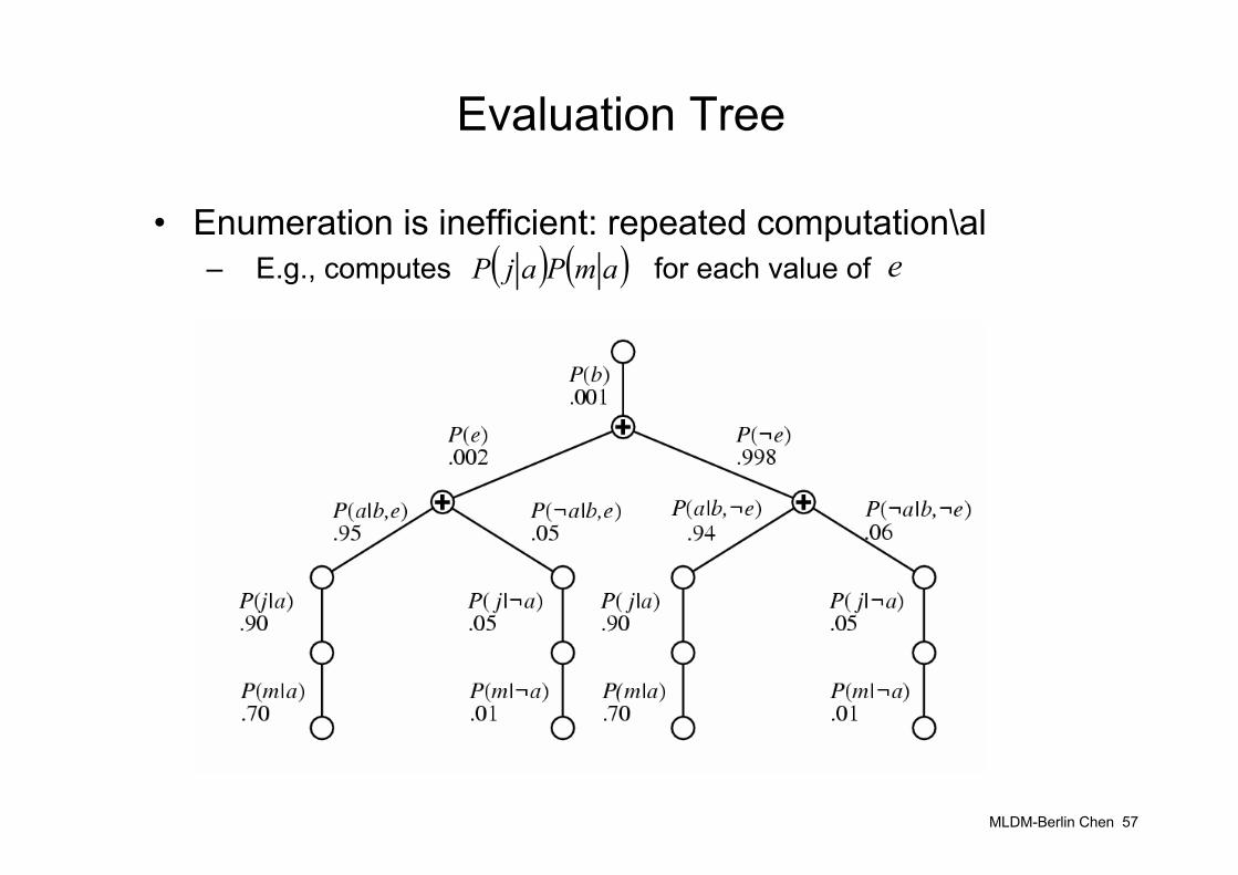
Evaluation Tree
• Enumeration is inefficient: repeated computation\al– E.g., computes for each value of ( ) ( )amPajP e
MLDM-Berlin Chen 58
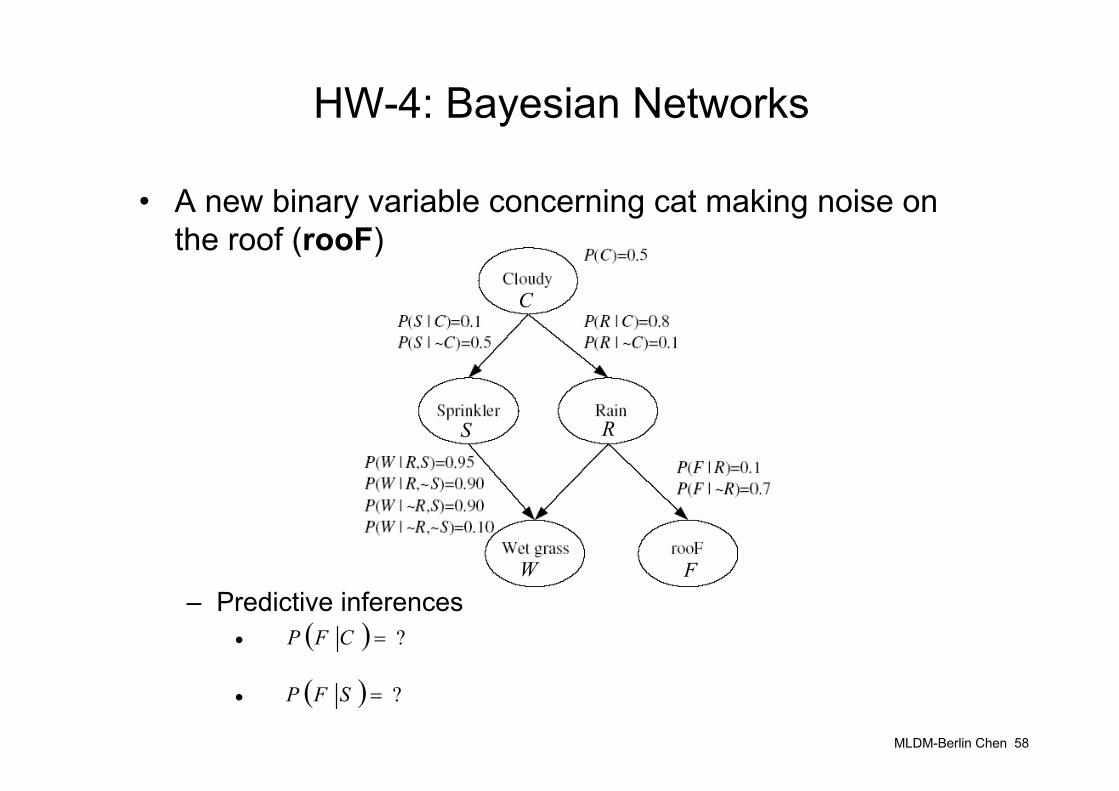
HW-4: Bayesian Networks
• A new binary variable concerning cat making noise on the roof (rooF)
– Predictive inferences•
•
( ) ?=CFP
( ) ?=SFP
FW
RS
C
MLDM-Berlin Chen 59
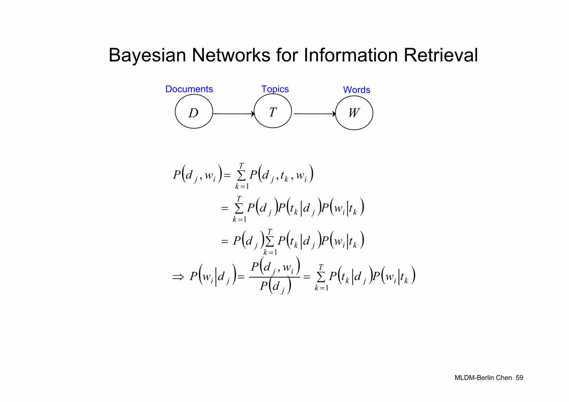
Bayesian Networks for Information Retrieval
D WT
( ) ( )
( ) ( ) ( )
( ) ( ) ( )
( ) ( )( ) ( ) ( )∑==⇒
∑=
∑=
∑=
=
=
=
=
T
kkijk
j
ijji
T
kkijkj
T
kkijkj
T
kikjij
twPdtPdP
wdPdwP
twPdtPdP
twPdtPdP
wtdPwdP
1
1
1
1
,
,,,
Documents Topics Words
MLDM-Berlin Chen 60
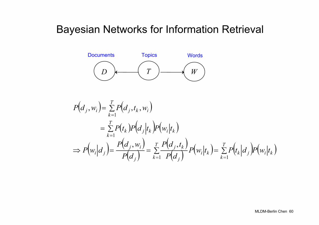
Bayesian Networks for Information Retrieval
D WT
( ) ( )
( ) ( ) ( )
( ) ( )( )
( )( ) ( ) ( ) ( )∑=∑==⇒
∑=
∑=
==
=
=
T
kkijk
T
kki
j
kj
j
ijji
T
kkikjk
T
kikjij
twPdtPtwPdP
tdPdP
wdPdwP
twPtdPtP
wtdPwdP
11
1
1
,,
,,,
Documents Topics Words