BAYESIAN APPROACH TO STRUCTURAL EQUATION MODELS FORORDERED CATEGORICAL AND DICHOTOMOUS DATA

THANOON Y. THANOON

A thesis submitted in fulfilment of therequirements for the award of the degree of

Doctor of Philosophy (Mathematics)

Faculty of ScienceUniversiti Teknologi Malaysia

FEBRUARY 2017

iii

To my beloved wife and my daughters Sara, Hajir and Maria

iv

ACKNOWLEDGEMENT

First of all, my praises and thanks to Almighty Allah, the Most Graciousthe Most Merciful, who gave me the knowledge, encouragement and patience toaccomplish this research. I wish to express my sincere appreciation and thanks tomy supervisor, Assoc. Prof. Dr. Robiah Adnan, for her encouragement when i haveproblems, guidance to the right way, and suggestions when i am hesitate, and criticalreviews of this thesis. Without her continued support and interest, this thesis would nothave been the same as presented here.

I am also indebted to Universiti Teknologi Malaysia (UTM) to give me a chanceto complete my PhD study and for the financial support for the Research UniversityGrant (Q.J130000 .2526. 06H68) and the Ministry of Higher Education (MOHE) ofMalaysia. I also need to take this opportunity to say thank you to the faculty of sciencestaff for their guidance, advice and knowledge in this field to help me successfullyfinished my thesis. Without their contribution, interest and guidance i would not beable to complete this study.

I owe my loving thanks to my wife, who has given me unlimited support andlove during my graduate study. I would also like to thank my beloved mother, father-in-law and mother-in-law, who have encouraged me to make my dreams come true. Itis because of all of you that i am the person i have become. Finally, many thanks aredue to everyone who helped me during my time at the Universiti Teknologi Malaysia.Many thanks to {Prof. Jichuan Wang} for advising the completion of this thesis andfor providing the data.

I would also like to thank my other committee members for their time andeffort. I am very thankful to all the staff in the department for their help. Last but notleast, i want to thank my family for their encouragement and support throughout mygraduate studies.

v

ABSTRACT

Structural equation modeling (SEM) is a statistical methodology that iscommonly used to study the relationships between manifest variables and latentvariables. In analysing ordered categorical and dichotomous data, the basic assumptionin SEM that the variables come from a continuous normal distribution is clearlyviolated. A rigorous analysis that takes into account the discrete nature of the variablesis therefore necessary. A better approach for assessing these kinds of discrete data isto treat them as observations that come from a hidden continuous normal distributionwith a threshold specification. A censored normal distribution and truncated normaldistribution, each includes interval, right and left where the later are with knownparameters, are used to handle the problem of ordered categorical and dichotomousdata in Bayesian non-linear SEMs. The truncated normal distribution is used tohandle the problem of non-normal data (ordered categorical and dichotomous) in thecovariates in the structural model. Two types of thresholds (having equal and unequalspaces) are used in this research. The Bayesian approach (Gibbs sampling method)is applied to estimate the parameters. SEM treats the latent variables as missing data,and imputes them as part of Markov chain Monte Carlo (MCMC) simulation results inthe full posterior distribution using data augmentation. An example using simulationdata, case study and bootstrapping method are presented to illustrate these methods.In addition to Bayesian estimation, this research provide the standard error estimates(SE), highest posterior density (HPD) intervals and a goodness-of-fit test using theDeviance Information Criterion (DIC) to compare with the proposed methods. Here, interms of parameter estimation and goodness-of-fit statistics, it is found that the resultswith a censored normal distribution are better than the results with a truncated normaldistribution, with equal and unequal spaces of thresholds. Furthermore, the results withunequal spaces of thresholds are less than the results of equal spaces of thresholds inthe interval of the censored and truncated normal distributions, this is including the leftcensored and truncated normal distributions. The results of equal spaces of thresholdsare less than the results of unequal spaces of thresholds in right censored and truncatednormal distributions. In other cases, the results of bootstrapping method are better thanthe real data results in terms of SE and DIC. The results of convergence showed thatdichotomous data needs more iterations to convergence than ordered categorical data.

vi

ABSTRAK

Pemodelan persamaan struktur (SEM) adalah suatu kaedah statistik yang

digunakan untuk mengkaji hubungan antara pembolehubah yang nyata dan

pembolehubah terpendam. Dalam menganalisis data berkategori turutan dan dikotomi,

andaian asas dalam SEM bahawa pembolehubah datang daripada taburan normal

selanjar jelas bercanggah. Oleh itu satu analisis teliti yang mengambil kira sifat

pembolehubah diskrit oleh itu adalah perlu. Pendekatan yang lebih baik untuk menilai

jenis data diskret yang seperti ini supaya dapat menanganinya adalah dengan

menganggapnya sebagai data yang datang daripada taburan normal selanjar

tersembunyi dengan nilai ambang yang spesifik. Taburan normal ditapis dan taburan

normal terpangkas dengan selang kanan dan kiri, dimana yang kemudian adalah

dengan parameter yang diketahui digunakan untuk menangani masalah kategori

turutan dan dikotomi dalam SEM Bayesan tidak linear. Taburan normal terpangkas

tersebut digunakan untuk menangani masalah data yang tidak normal (data

berkategori turutan dan dikotomi) dalam covariates model struktur. Dua jenis nilai

ambang (mempunyai ruang yang sama dan yang tidak sama) digunakan dalam kajian

ini. Pendekatan Bayesan (kaedah persampelan Gibbs) digunakan untuk

menganggarkan parameter. SEM menangani pembolehubah terpendam sebagai data

hilang, dan ia digunakan bagi melengkapkan keputusan simulasi Monte Carlo rantaian

Markov (MCMC) untuk taburan posterior penuh dengan menggunakan pembesaran

data. Satu contoh yang menggunakan data simulasi, kajian kes dan kaedah

bootstrapping akan dibentangkan untuk menggambarkan kaedah-kaedah ini. Sebagai

tambahan kepada anggaran Bayesan, kajian ini menyediakan anggaran ralat piawai

(SE), selang ketumpatan posterior tertinggi (HPD) dan ujian kebagusan penyesuaian

yang menggunakan Devians Kiteria Maklumat (DIC), digunakan sebagai

perbandingan dengan kaedah yang dicadangkan. Dari segi anggaran parameter dan

statistik kebagusan penyesuaian, didapati keputusan taburan normal ditapis adalah

lebih baik daripada keputusan taburan normal terpangkas, bagi ruang yang sama dan

tidak sama untuk nilai ambang. Tambahan pula, keputusan dengan ruang yang tidak

sama bagi nilai ambang adalah kurang daripada keputusan untuk ruang sama bagi

nilai ambang dalam selang untuk taburan normal ditapis dan dipangkas, ini

termasuklah taburan normal ditapis kiri dan terpangkas. Keputusan bagi ruang sama

untuk nilai ambang adalah kurang berbanding keputusan bagi ruang yang tidak sama

untuk nilai ambang dalam taburan normal ditapis kanan dan terpangkas. Dalam kes

lain, keputusan bagi kaedah bootstrapping adalah lebih baik daripada data sebenar

dari segi SE dan DIC. Keputusan penumpuan menunjukkan bahawa data dikotomi

memerlukan lebih banyak lelaran untuk menumpu berbanding data berkategori

turutan.

vii

TABLE OF CONTENTS

CHAPTER TITLE PAGE

DECLARATION iiDEDICATION iiiACKNOWLEDGEMENT ivABSTRACT vABSTRAK viTABLE OF CONTENTS viiLIST OF TABLES xiLIST OF FIGURES xivLIST OF ABBREVIATIONS xviiLIST OF SYMBOLS xixLIST OF APPENDICES xxi

1 INTRODUCTION 11.1 Problem Statement 31.2 Objectives of the Study 41.3 Scope of the Study 51.4 The Significance of the Research 51.5 The Organization of Thesis 6

2 LITERATURE REVIEW 82.1 The Introduction 82.2 Non-linear Structural Equation Models 122.3 Structural Equation Models for Ordered Categorical

and Dichotomous Variables 132.4 The Bayesian Analysis of Structural Equation

Models 172.5 Using Bayesian Analysis to Investigate Structural

Equation Models with Dichotomous Variables 21

viii

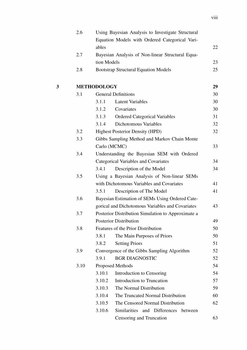
2.6 Using Bayesian Analysis to Investigate StructuralEquation Models with Ordered Categorical Vari-ables 22

2.7 Bayesian Analysis of Non-linear Structural Equa-tion Models 23

2.8 Bootstrap Structural Equation Models 25

3 METHODOLOGY 293.1 General Definitions 30

3.1.1 Latent Variables 303.1.2 Covariates 303.1.3 Ordered Categorical Variables 313.1.4 Dichotomous Variables 32

3.2 Highest Posterior Density (HPD) 323.3 Gibbs Sampling Method and Markov Chain Monte

Carlo (MCMC) 333.4 Understanding the Bayesian SEM with Ordered

Categorical Variables and Covariates 343.4.1 Description of the Model 34

3.5 Using a Bayesian Analysis of Non-linear SEMswith Dichotomous Variables and Covariates 413.5.1 Description of The Model 41

3.6 Bayesian Estimation of SEMs Using Ordered Cate-gorical and Dichotomous Variables and Covariates 43

3.7 Posterior Distribution Simulation to Approximate aPosterior Distribution 49

3.8 Features of the Prior Distribution 503.8.1 The Main Purposes of Priors 503.8.2 Setting Priors 51

3.9 Convergence of the Gibbs Sampling Algorithm 523.9.1 BGR DIAGNOSTIC 52

3.10 Proposed Methods 543.10.1 Introduction to Censoring 543.10.2 Introduction to Truncation 573.10.3 The Normal Distribution 593.10.4 The Truncated Normal Distribution 603.10.5 The Censored Normal Distribution 623.10.6 Similarities and Differences between

Censoring and Truncation 63

ix

3.10.7 Censoring and Truncation Using BUGSPrograms 64

3.11 Data Augmentation 653.12 Model Comparison 66

4 SIMULATION STUDY 694.1 Overview 694.2 Sample Size for SEMs 704.3 Analysis of Simulated Data 714.4 The Results of Censored Normal Distribution 74

4.4.1 Simulation Results and Discussion ofBNSEMs for Ordered Categorical DataUsing Censored Normal Distribution withEqual and Unequal Spaces of Thresholdsas the Following 74

4.4.2 Simulation Results and Discussion ofBNSEMs for Dichotomous Data UsingCensored Normal Distribution with EqualSpaces of Thresholds as the Following 86

4.5 The Results of Truncated Normal Distribution 934.5.1 Simulation Results and Discussion of

BNSEMs for Ordered Categorical DataUsing Truncated Normal Distributionwith Equal and Unequal Spaces ofThresholds as the Following 93

4.5.2 Simulation Results and Discussion ofBNSEMs for Dichotomous Data Us-ing Truncated Normal Distribution withEqual Spaces of Thresholds 105

4.5.3 Goodness of Fit Statistics Results forCensored Normal Distribution with Equaland Unequal Spaces of Thresholds 111

4.5.4 Goodness of Fit Statistics Results forTruncated Normal Distribution withEqual and Unequal Spaces of Thresholds 113

5 A CASE STUDY 1175.1 Real Example for Ordered Categorical Data 117

xi

LIST OF TABLES

TABLE NO. TITLE PAGE

3.1 Cross-Tabulation of Two Ordered Categorical Variables Xand Y 40

3.2 Cross-Tabulation of Two Dichotomous Variables X and Y 434.1 Bayesian Estimation of NSEMs for Ordered Categorical Data

Using Interval Censored Normal Distribution with EqualSpaces of Thresholds 74

4.2 Bayesian Estimation of NSEMs for Ordered Categorical DataUsing Interval Censored Normal Distribution with UnequalSpaces of Thresholds 75

4.3 Bayesian Estimation of NSEMs for Ordered CategoricalData Using Right Censored Normal Distribution with EqualSpaces of Thresholds 78

4.4 Bayesian Estimation of NSEMs for Ordered Categorical DataUsing Left Censored Normal Distribution with Equal Spacesof Thresholds 79

4.5 Bayesian Estimation of NSEMs for Ordered Categorical DataUsing Right Censored Normal Distribution with UnequalSpaces of Thresholds 80

4.6 Bayesian Estimation of NSEMs for Ordered CategoricalData Using Left Censored Normal Distribution with UnequalSpaces of Thresholds 81

4.7 Bayesian Estimation of NSEMs for Dichotomous Data UsingInterval Censored Normal Distribution with Equal Spaces ofThresholds 86

4.8 Bayesian Estimation of NSEMs for Dichotomous Data UsingRight Censored Normal Distribution 89

4.9 Bayesian Estimation of NSEMs for Dichotomous Data UsingLeft Censored Normal Distribution 90

xii

4.10 Bayesian Estimation of NSEMs for Ordered Categorical DataUsing Interval Truncated Normal Distribution with EqualSpaces of Thresholds 93

4.11 Bayesian Estimation of Non-linear SEMs for Ordered Cat-egorical Data Using Interval Truncated Normal Distributionwith Unequal Spaces of Thresholds 94

4.12 Bayesian Estimation of NSEMs for Ordered CategoricalData Using Right Truncated Normal Distribution with EqualSpaces of Thresholds 97

4.13 Bayesian Estimation of NSEMs for Ordered Categorical DataUsing Left Truncated Normal Distribution with Equal Spacesof Thresholds 98

4.14 Bayesian Estimation of NSEMs for Ordered Categorical DataUsing Right Truncated Normal Distribution with UnequalSpaces of Thresholds 99

4.15 Bayesian Estimation of Nonlinear SEMs for OrderedCategorical Data Using Left Truncated Normal Distributionwith Unequal Spaces of Thresholds 100

4.16 Bayesian Estimation of NSEMs for Dichotomous Data UsingInterval Truncated Normal Distribution with Equal Spaces ofThresholds 105

4.17 Bayesian Estimation of NSEMs for Dichotomous Data UsingRight Truncated Normal Distribution 107

4.18 Bayesian Estimation of NSEMs for Dichotomous Data UsingLeft Truncated Normal Distribution 108

4.19 Performance of Deviance Information Criterion (DIC) forBNSEMs with Equal Spaces of Thresholds Using IntervalCensored Normal Distribution 111

4.20 Performance of Deviance Information Criterion (DIC) forBNSEMs with Equal Spaces of Thresholds Using RightCensored Normal Distribution 111

4.21 Performance of Deviance Information Criterion (DIC) forBNSEMs with Equal Spaces of Thresholds Using LeftCensored Normal Distribution 111

4.22 Performance of Deviance Information Criterion (DIC) forBNSEMs with Unequal Spaces of Thresholds Using IntervalCensored Normal Distribution 112

xiii

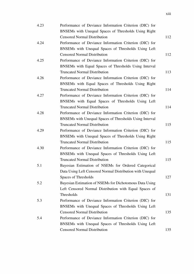
4.23 Performance of Deviance Information Criterion (DIC) forBNSEMs with Unequal Spaces of Thresholds Using RightCensored Normal Distribution 112

4.24 Performance of Deviance Information Criterion (DIC) forBNSEMs with Unequal Spaces of Thresholds Using LeftCensored Normal Distribution 112

4.25 Performance of Deviance Information Criterion (DIC) forBNSEMs with Equal Spaces of Thresholds Using IntervalTruncated Normal Distribution 113

4.26 Performance of Deviance Information Criterion (DIC) forBNSEMs with Equal Spaces of Thresholds Using RightTruncated Normal Distribution 114

4.27 Performance of Deviance Information Criterion (DIC) forBNSEMs with Equal Spaces of Thresholds Using LeftTruncated Normal Distribution 114

4.28 Performance of Deviance Information Criterion (DIC) forBNSEMs with Unequal Spaces of Thresholds Using IntervalTruncated Normal Distribution 115

4.29 Performance of Deviance Information Criterion (DIC) forBNSEMs with Unequal Spaces of Thresholds Using RightTruncated Normal Distribution 115

4.30 Performance of Deviance Information Criterion (DIC) forBNSEMs with Unequal Spaces of Thresholds Using LeftTruncated Normal Distribution 115

5.1 Bayesian Estimation of NSEMs for Ordered CategoricalData Using Left Censored Normal Distribution with UnequalSpaces of Thresholds 127

5.2 Bayesian Estimation of NSEMs for Dichotomous Data UsingLeft Censored Normal Distribution with Equal Spaces ofThresholds 131

5.3 Performance of Deviance Information Criterion (DIC) forBNSEMs with Unequal Spaces of Thresholds Using LeftCensored Normal Distribution 135

5.4 Performance of Deviance Information Criterion (DIC) forBNSEMs with Unequal Spaces of Thresholds Using LeftCensored Normal Distribution 135

xiv

LIST OF FIGURES

FIGURE NO. TITLE PAGE

2.1 Flow Chart of the Study 283.1 Path Diagram of Non-linear Structural Model 373.2 The hidden continuous normal distribution with a thresholds

specification 403.3 The hidden continuous normal distribution with a single of

threshold fixed at zero 433.4 The Normal Distribution with Truncation and Censoring 603.5 Latent, Censored, and Truncation Variables 643.6 Flow Chart of the Proposed Methods 684.1 The Path Diagram of Non-linear SEMs (M4) for the

Simulation Data 724.2 Plots of BGR Diagnostic of λ1, λ2, β2, β3, and γ3 for M4

with Ordered Categorical Data Using Interval Censoring withEqual Spaces of Thresholds and n=200 76

4.3 Plots of BGR Diagnostic of β1, β3, β4, λ2 and λ4 for M4

with Ordered Categorical Data Using Interval Censoring withUnequal Spaces of Thresholds and n=200 77

4.4 Plots of BGR Diagnostic of λ3, λ2, β3, γ1, and γ3 for M4 withOrdered Categorical Data Using Right Censoring with EqualSpaces of Thresholds and n=200 82

4.5 Plots of BGR Diagnostic of λ3, λ4, γ2, γ3, and β4 for M4 withOrdered Categorical Data Using Left Censoring with EqualSpaces of Thresholds and n=200 83

4.6 Plots of BGR Diagnostic of β2, γ3, β4, γ2, and ψεδ for M4

with Ordered Categorical Data Using Right Censoring withUnequal Spaces of Thresholds and n=200 84

4.7 Plots of BGR Diagnostic of λ1, γ3, λ4, β2, and γ2 for M4 withOrdered Categorical Data Using Left Censoring with UnequalSpaces of Thresholds and n=200 85

xv

4.8 Plots of BGR Diagnostic of λ3, λ4, λ2, β2, and γ1 forM4 with Dichotomous data Using Interval Censored NormalDistribution with Equal Spaces of Thresholds and n=200 88

4.9 Plots of BGR Diagnostic of λ1, γ3, λ3, λ4, and β2 forM4 with Dichotomous Data Using Right Censored NormalDistribution with Equal Spaces of Thresholds and n=200 91

4.10 Plots of BGR Diagnostic of β4, γ1, λ4, λ6, and γ3 for M4 withDichotomous Data Left Censored Normal Distribution withEqual Spaces of Thresholds and n=200 92

4.11 Plots of BGR Diagnostic of γ1, λ2, λ1, λ6, and Φ22 forM4 with Ordered Categorical Data Using Interval Truncationwith Equal Spaces of Thresholds and n=200 95

4.12 Plots of BGR Diagnostic of λ5, λ6, λ1, λ3, and β4 for M4

with Ordered Categorical Data Using Interval Truncationwith Unequal Spaces of Thresholds and n=200 96

4.13 Plots of BGR Diagnostic of λ4, β4, λ1, λ5, and γ3 for M4 withOrdered Categorical Data Using Right Truncation with EqualSpaces of Thresholds and n=200 101

4.14 Plots of BGR Diagnostic of λ3, λ6, λ5, β4, and γ1 for M4 withOrdered Categorical Data Using Left Truncation with EqualSpaces of Thresholds and n=200 102

4.15 Plots of BGR Diagnostic of λ2, λ3, λ4, λ5, and β4 for M4

with Ordered Categorical Data Using Right Truncation withUnequal Spaces of Thresholds and n=200 103

4.16 Plots of BGR Diagnostic of β4, γ3, λ3, λ6, and β2 for M4

with Ordered Categorical Data Using Left Truncation withUnequal Spaces of Thresholds and n=200 104

4.17 Plots of BGR Diagnostic of γ1, λ2, λ4, β1, and β2 for M4

with Dichotomous Data Using Interval Truncated NormalDistribution with Equal Spaces of Thresholds and n=200 106

4.18 Plots of BGR Diagnostic of λ2, β2, λ3, λ4, and β4 forM4 with Dichotomous Data Using Right Truncated NormalDistribution with Equal Spaces of Thresholds and n=200 109

4.19 Plots of BGR Diagnostic of λ1, λ4, λ2, λ3, and γ2 forM4 withDichotomous Data Using Left Truncated Normal Distributionwith Equal Spaces of Thresholds and n=200 110

5.1 The path diagram of non-linear SEMs (M4) for Real Data(Dichotomous) 125

xvi

5.2 Plots of BGR Diagnostic of λ1, λ2, λ5, λ9, and λ12 for M4

with Real Data (Ordered Categorical) Using Left CensoredNormal Distribution with Unequal Spaces of Thresholds 129

5.3 Plots of BGR Diagnostic of λ5, λ7, λ8, λ10, and β1

for M4 with bootstrapping (Ordered Categorical) UsingLeft Censored Normal Distribution with Unequal Spaces ofThresholds 130

5.4 Plots of BGR Diagnostic of λ3, λ5, β3, β4, and γ3 for M4

with Real data (Dichotomous) using Left Censored NormalDistribution and Equal Spaces of Thresholds 132

5.5 Plots of BGR Diagnostic of λ4, λ5, γ2, γ3, and β4 for M4

with bootstrapping Method for (Dichotomous Data) usingLeft Censored Normal Distribution and Equal Spaces ofThresholds 133

5.6 Path Diagram of Psychological Data with Non-linear SEMfor Ordered Categorical Data (M4) 136

xvii

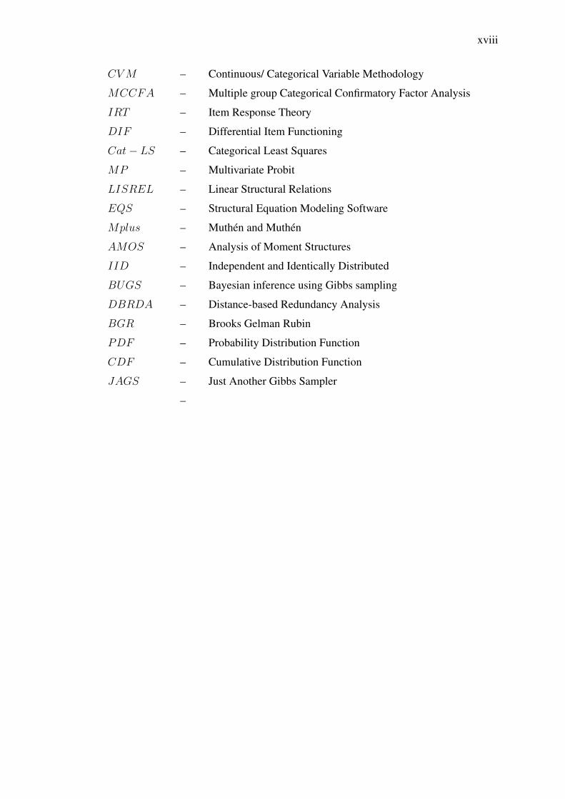
LIST OF ABBREVIATIONS

SEM – Structural Equation Modeling

SEMs – Structural Equation Models

NSEMs – Nonlinear Structural Equation Models

BSEMs – Bayesian Structural Equation Models

BNSEMs – Bayesian Nonlinear Structural Equation Models

PP – Posterior Predictive

ESEM – Exploratory Structural Equation Modeling

FA – Factor Analysis

EFA – Exploratory Factor Analysis

CFA – Confirmatory Factor Analysis

MCMC – Markov chain Monte Carlo

HPD – Highest Posterior Density

DIC – Deviance Information Creterion

AIC – Akaike Information Creterion

BF – Bayes Factor

BIC – Bayesian Information Creterion

WLS – Weighted Least Squares

ML – Maximum Likelihood

WLSMV – Weighted Least Squares with Mean and Variance Adjusted

MLR – Robust Maximum Likelihood

GLS – Generalized Least Squares

ULS – Unweighted Least Squares

MLMV – Maximum Likelihood with Mean and Variance Adjusted

MLM – Maximum Likelihood with Mean Adjusted

ADF – Asymptotically Distribution Free

PLS – Partial Least Square

GLLAMM – Generalized Linear Latent and Mixed Models

GLMM – Generalized Linear Mixed Models

xviii

CVM – Continuous/ Categorical Variable Methodology

MCCFA – Multiple group Categorical Confirmatory Factor Analysis

IRT – Item Response Theory

DIF – Differential Item Functioning

Cat− LS – Categorical Least Squares

MP – Multivariate Probit

LISREL – Linear Structural Relations

EQS – Structural Equation Modeling Software

Mplus – Muthén and Muthén

AMOS – Analysis of Moment Structures

IID – Independent and Identically Distributed

BUGS – Bayesian inference using Gibbs sampling

DBRDA – Distance-based Redundancy Analysis

BGR – Brooks Gelman Rubin

PDF – Probability Distribution Function

CDF – Cumulative Distribution Function

JAGS – Just Another Gibbs Sampler

–

xix

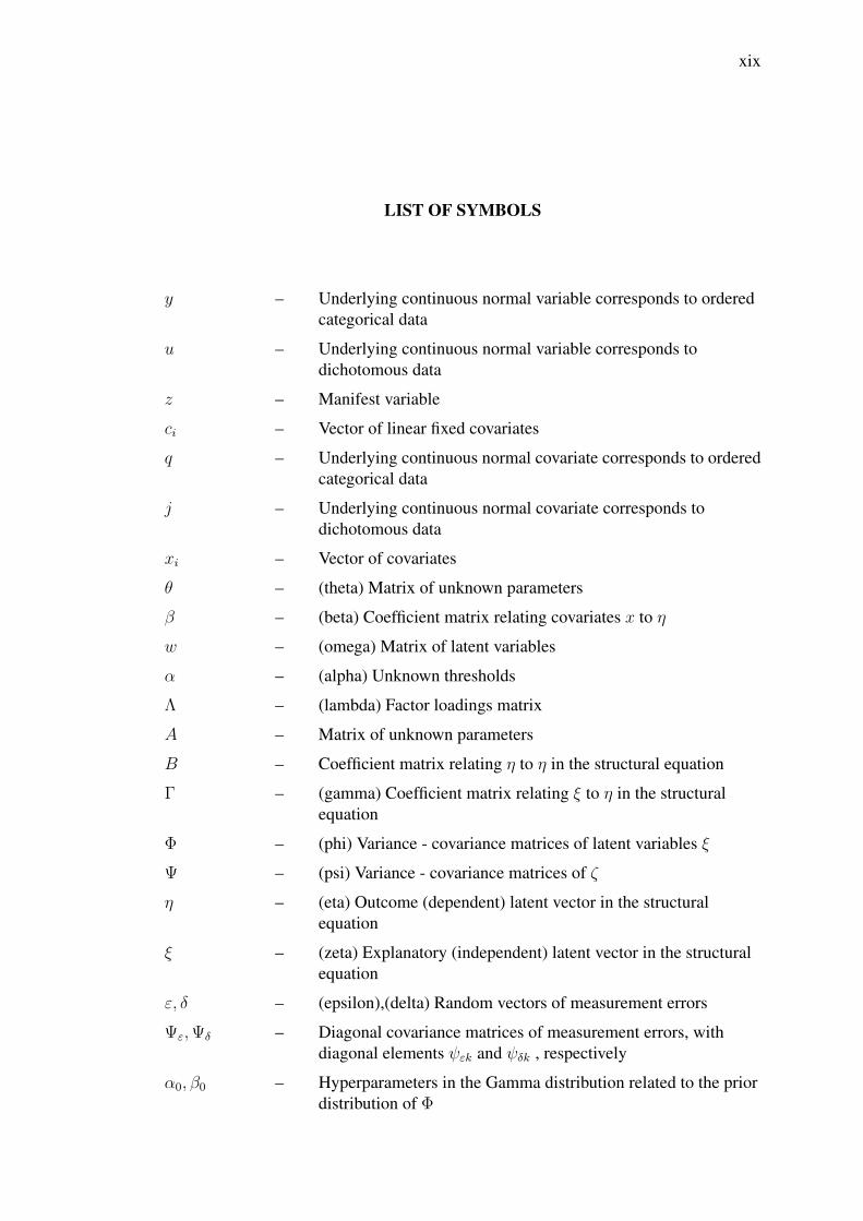
LIST OF SYMBOLS

y – Underlying continuous normal variable corresponds to orderedcategorical data

u – Underlying continuous normal variable corresponds todichotomous data

z – Manifest variable

ci – Vector of linear fixed covariates

q – Underlying continuous normal covariate corresponds to orderedcategorical data

j – Underlying continuous normal covariate corresponds todichotomous data

xi – Vector of covariates

θ – (theta) Matrix of unknown parameters

β – (beta) Coefficient matrix relating covariates x to η

w – (omega) Matrix of latent variables

α – (alpha) Unknown thresholds

Λ – (lambda) Factor loadings matrix

A – Matrix of unknown parameters

B – Coefficient matrix relating η to η in the structural equation

Γ – (gamma) Coefficient matrix relating ξ to η in the structuralequation

Φ – (phi) Variance - covariance matrices of latent variables ξ

Ψ – (psi) Variance - covariance matrices of ζ

η – (eta) Outcome (dependent) latent vector in the structuralequation

ξ – (zeta) Explanatory (independent) latent vector in the structuralequation

ε, δ – (epsilon),(delta) Random vectors of measurement errors

Ψε,Ψδ – Diagonal covariance matrices of measurement errors, withdiagonal elements ψεk and ψδk , respectively

α0, β0 – Hyperparameters in the Gamma distribution related to the priordistribution of Φ

xx

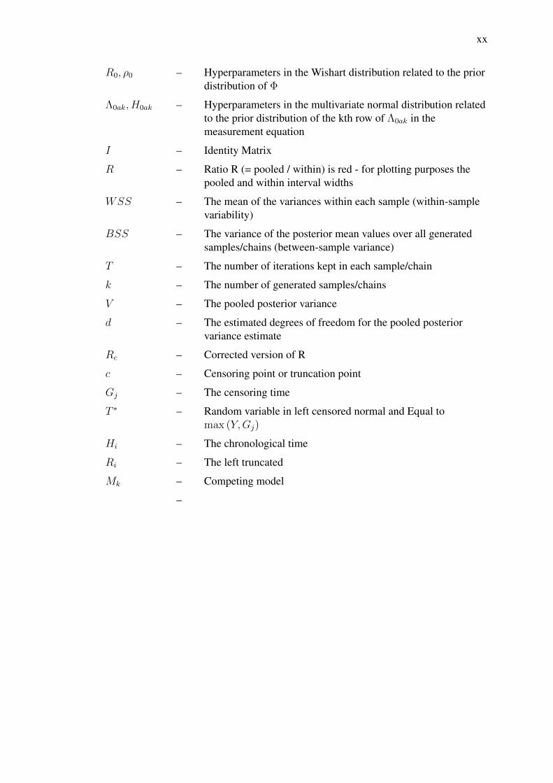
R0, ρ0 – Hyperparameters in the Wishart distribution related to the priordistribution of Φ

Λ0ak, H0ak – Hyperparameters in the multivariate normal distribution relatedto the prior distribution of the kth row of Λ0ak in themeasurement equation

I – Identity Matrix

R – Ratio R (= pooled / within) is red - for plotting purposes thepooled and within interval widths

WSS – The mean of the variances within each sample (within-samplevariability)

BSS – The variance of the posterior mean values over all generatedsamples/chains (between-sample variance)

T – The number of iterations kept in each sample/chain

k – The number of generated samples/chains

V – The pooled posterior variance

d – The estimated degrees of freedom for the pooled posteriorvariance estimate

Rc – Corrected version of R

c – Censoring point or truncation point

Gj – The censoring time

T ∗ – Random variable in left censored normal and Equal tomax (Y,Gj)

Hi – The chronological time

Ri – The left truncated

Mk – Competing model

–

xxi

LIST OF APPENDICES

APPENDIX TITLE PAGE

A Published and Accepted Papers 152

CHAPTER 1

INTRODUCTION

This chapter contains a brief introduction to Bayesian structural equationmodels (BSEMs) with linear fixed covariates and exogenous latent variables in themeasurement model and non-linear covariates and exogenous latent variables in thestructural model. Ordered categorical and dichotomous data are used in this research.Analysing data necessitates a determination of the type of data being analysed.However, there are many types of distributions; the most basic distribution of thedata is the normal distribution. The similarity between the distribution of the dataand the distribution assumed in the analysis can affect the validity of the result.It is not a good idea to assume the distribution of the dependent variables andthe covariates to be normal when using ordered categorical and dichotomous data.However, routinely treating these types of data as coming from a normal distributionmay lead to erroneous results. Structural equation models (SEMs) always assume thatthe dependent variables are normally distributed. In addition, the ordered categoricaland dichotomous variables and covariates are assumed to be normally distributedwhen, in fact, they are discrete variables and covariates. Finally, ordered categoricaland dichotomous variables and covariates often display positive or negative skew, suchthat the frequency for low counts is higher than the frequency when the count levelincreases, or the frequency for low counts is lower than that for high counts. A moreappropriate analysis includes the specification of a censored normal distribution ora truncated normal distribution with known parameters and thresholds specification,rather than a normal distribution.

There are two main types of structural equation models, the first, is classicalstructural equation models which include maximum likelihood method (ML) andweighted least square method (WLS). The second, is Bayesian structural equationmodels such as Gibbs sampling method. However, in this thesis, we will focus onBayesian SEMs using Gibbs sampling method.

2

Ordered categorical data are those with more than two categories, whiledichotomous data are those with only two categories. Two types of distributions thatused in this research, hidden continuous normal distribution are proposed for handlingthe problem of non-normal data in variables and covariates (ordered categorical anddichotomous). The hidden continuous normal distribution considered in this researchare censored normal distribution and truncated normal distribution with knownparameters. The choice between the models depends on the parameter estimationresults and the goodness-of-fit statistics, Deviance Information Criterion (DIC). Inmany applications, the ordered categorical and dichotomous response variable dataare from a complete data set. In this research, the focus is on the unobserved data thatare hidden continuous normal data (censored and truncated normal distribution data).There are many researches that are carried out using structural equation models withfull data. Thus, the likelihood function for a censored or truncated structural equationmodel is not the same as the likelihood function of a structural equation model withfull data.

As we have seen, there is a great deal of research about Bayesian structuralequation models; we can also find studies about ordered categorical and dichotomousdata. However, there has been no research on BSEMs with linear fixed covariatesand latent variables in the measurement model and non-linear covariates and latentvariables in the structural model, for ordered categorical and dichotomous variablesand covariates. The response variables in a Bayesian structural equation model forordered categorical and dichotomous variables and covariates with unobserved data,however, there is not sufficient information for the over-dispersion problem in a normaldistribution in the BSEMs. We are interested in discussing models with this kind ofdata, since the dependent variables are ordered categorical or dichotomous variablesand covariates. Thresholds (cut points) are used to change the ordered categoricaland dichotomous data to the continuous normal data in the variables and covariatesusing underlying continuous normal distribution. Therefore, when talking aboutBSEMs with unobserved data, that means a hidden continuous normal distributionwith censoring or truncation.

Real data usually does not completely satisfy the assumptions often madeby researches which result in a dramatic effect on the quality of statistical analysis.The developement of bootstrap estimation technique has become very competitive forimprovng the efficiency of parameters in structural equation models. Bootstrap isa method for assigning measures of accuracy to sample estimates. The techniquesare more than 30 years old and were first introduced by Efron (1979). The basic

3

idea of bootstrap method is to generate observations that are randomly drawn withreplacement from the original data set. The set of the selected sub-samples areconsidered as bootstrap samples and can be used to estimate the parameters ofstructural equation models. The bootstrap method obtained from such procedure iscalled pair bootstrap. However, these bootstraps are computer intensive method thatcan replace the theoretical formulation. The attractive feature of bootstrap methodis that it does not rely on the assumption of normal distribution and is capable ofestimating the standard error of any complicated estimator without any theoreticalcalculations. The interesting properties of the bootstrap techniques have to be tradedoff with computation cost and time (Rana et al., 2012).

1.1 Problem Statement

Several models and methods have been proposed in the past for analysingBSEMs with ordered categorical and dichotomous data. For instance, Song andLee (2006a) proposed Bayesian structural equation models with non-linear covariatesand latent variables in the structural model, with mixed continuous and dichotomousdata, and they treated the dichotomous data in the covariates as a continuous normaldistribution. A truncated normal distribution with unknown parameters was usedto handle the problem of dichotomous data. The posterior predictive (PP) p-valuewas used as a goodness-of-fit statistics for model comparison. Lee (2007) used ahidden continuous normal distribution (truncated normal distribution) with unknownparameters to handle the problem of ordered categorical data. Lunn et al. (2009)and Lunn et al. (2012) mentioned that the truncated normal distribution is to be usedonly if there are no unknown parameters or if a censored prior distribution has beenspecified for the parameters. However, the truncated normal distribution is used whenthe dependent variables contain observed data only or when the dependent variablescontain some unobserved data with no unknown parameters. Lu et al. (2012) usedcontinuous normal distribution as a proposed method to handle the problem of orderedcategorical variables in BSEMs, with an application to behavioral finance. In thisthesis, the first problem is how to handle the problem of non-normal data (orderedcategorical variables) in Bayesian non-linear SEMs to the measurement model . Thesecond problem is how to improve the performance of Bayesian non-linear SEMs whenthere are non-normal data (dichotomous) in the variables in the measurement model.The third problem is how to find Bayesian analysis of non-linear structural equationmodels when there are (ordered categorical and dichotomous data) in the covariates inthe structural model.

4

1.2 Objectives of the Study

A number of studies have presented applications of the analysis of Bayesianstructural equation models with non-normal data. Most of these researches haveconsidered hidden continuous normal distribution (truncated normal distribution withunknown parameters) for the data. The aim of this study is to discuss the problems ofordered categorical and dichotomous data and also covariates in these models, whichmeans that we are going to discuss Bayesian non-linear structural equation models(BNSEMs) as a tool for the analysis of ordered categorical and dichotomous data withunobserved data in variables and covariates. This study embarks on the followingobjectives:

1. To handle the problem of ordered categorical variables in the measurementmodel, using a hidden continuous normal distribution (interval censored normaldistribution, right and left censoring) and (interval truncated normal distribution,right and left truncation) with two types of thresholds (with equal and unequalspaces).

2. To improve the performance of BNSEMs with dichotomous variables using ahidden continuous normal distribution (interval censored normal distribution,right and left censoring) and (interval truncated normal distribution, right andleft truncation) with known parameters and one type of thresholds (with equalspaces).

3. To handle the problem of non-normal data (ordered categorical anddichotomous) for the covariates in the structural model using an intervaltruncated normal distribution, and right truncation and left truncation with twotypes of thresholds (with equal and unequal spaces) for ordered categorical dataand one type of thresholds (with equal spaces) for dichotomous data.

4. To evaluate the performance of the proposed methods when dealing with orderedcategorical and dichotomous variables and covariates, through simulation, a casestudy and bootstrapping method. Comparisons are made based on goodness-of-fit statistics using Deviance Information Criterion (DIC).

5

1.3 Scope of the Study

In this research, we discuss BNSEMs with non-linear covariates and latentvariables for ordered categorical and dichotomous variables and covariates. The focusis on hidden continuous normal distribution methods, with both censored normaldistribution (which includes interval, right and left censoring) and truncated normaldistribution (which includes interval, right and left truncation) with known parameters,to handle the problem of ordered categorical and dichotomous variables. Furthermore,three different kinds of truncation – interval, right and left truncation with knownparameters are going to handle the problem of discrete data in the covariates. TheGibbs sampling method is used to perform the parameter estimation for the proposedmodels. It will discuss the previous models in the simulation study and apply theproposed methods to simulated data by using the R-program, and analyse these usingthe R2OpenBUGS package in the R-program. First, the simulated data is made upof SEMs with ordered categorical variables and covariates. The second simulationinvolves data with SEMs and dichotomous variables and covariates. One sample size(n=200), two different initial values and two different types of thresholds (with equaland unequal spaces) for ordered categorical data and one type of thresholds (with equalspaces) for dichotomous data will be considered, to investigate the effects of differentsample sizes and different initial values on the proposed methods. The proposedmethods (left censored normal distribution with unequally spaces of thresholds forordered categorical data, and left censored normal distribution with equally spaces ofthresholds for dichotomous data) will be applied to a case study and bootstrappingmethod (resampling the real data) with SEMs for ordered categorical and dichotomousvariables and covariates with sample size n=200. The non-linear models are selected inthis research using a combination between covariates and exogenous latent variables.Quadratic and cubic effects are used in the proposed models to explain the non-lineareffects on the endogenous latent variables.

1.4 The Significance of the Research

Analysis of structural equation models is very important since these modelsare used in many fields, including scientific, social and behavioral sciences. Manyresearchers have proposed methods to obtain accurate estimates of parameters fordifferent types of variables. This research focuses on the problem of orderedcategorical and dichotomous data in variables and covariates in Bayesian non-linearstructural equation models. The focus is to determine which of the proposed methods

6

is the best for estimating the parameters of the models. The best model can beidentified by using the statistical error measurements such as standard error (SE) andhighest posterior density (HPD). The Deviance Information Criterion (DIC) is usedas a goodness-of-fit statistic to compare the performance of the proposed models. Tohandle the problems referred to above, we use a hidden continuous normal distribution(censored and truncated normal distribution) in Bayesian analysis with a Markov chainMonte Carlo (MCMC) simulation method for analysing non-linear structural equationmodels. In this approach, the standard error estimates (SE) can easily be obtainedthrough simulated observations from the joint posterior distribution by the MCMCmethods, and the Bayesian analysis can be conducted in SEM by using the OpenBUGSprogram and R2OpenBUGS package in the R-program. The Gibbs sampler algorithmis used to implement the Bayesian SEMs. The Bayesian SEM methodology permitsthe user to utilize the prior information for updating the current information on theparameter. This research provides the parameter estimation, standard error (SE),highest posterior density (HPD) and the goodness-of-fit statistics (DIC) of the proposedmodels, and these results can help researchers in determining the appropriate modelwith ordered categorical and dichotomous data in variables and covariates.

1.5 The Organization of Thesis

The goal of this research is to introduce some new methods to handle theproblem of ordered categorical and dichotomous data in variables and covariates inBayesian non-linear structural equation models. The proposed research work has beenintroduced, with an overview, a statement of the problem, objectives, scope and thesignificance of the research. The research study deals with the problem of orderedcategorical and dichotomous variables and covariates in Bayesian structural equationmodels. To reach this goal, an improved approach was proposed that will enable us tohandle the problem of these types of variables, based on the objectives that have beendefined in this chapter.

The rest of the work is organized as follows: Chapter 2 reviews the relevantliterature, including research related to structural equation models (SEMs), non-linearSEMs, Bayesian SEMs, classical and Bayesian SEMs with ordered categorical anddichotomous variables, Bayesian non-linear SEMs, and Bootstrap SEMs. In Chapter3, we present our methodology, which uses Bayesian structural equation models withnon-linear covariates and latent variables for ordered categorical and dichotomous datain variables and covariates. We also present some proposed methods. Chapter 4

65

through the T(,) construct, whose syntax is the same as that of the I(,) construct inOpenBUGS. However, the interpretation is different. The I(,) mechanism throughwhich censored data is dealt with, cannot be used for modeling truncated distribution aslong as they lack unknown parameters. In case there are parameters that are unknown,then there will be wrong inferences. Hence, the I(,) construct does not work wellfor truncated distribution where there are unknown parameters. Nonetheless, theI(,) construct is necessary for making truncated distribution with known parameters(Plummer, 2012).

3.11 Data Augmentation

Data augmentation, which occurs as the result of latent or auxiliary variables, isa method of converting the unobserved variable to more usable form, like usual linearregression. This allows the Gibbs sampler to be used, and simplifies calculation. Onereason why data augmentation is used, is to ensure that the conjugacy of the prior andthe likelihood will regulate the posterior, allowing it to take a standard form. As aresult, it can be used to simplify sample collection in discrete mixture models, and alsoforms the foundation for using the missing data model (Congdon, 2005).

The concept of data augmentation comes from missing value problems, asdemonstrated by its similarity to missing cells in balanced two-way tables. From aBayesian perspective, the posterior distribution of the parameter of interest shouldbe calculated. This can be accomplished through data augmentation, maximisingthe likelihood estimate, and computing the posterior distribution. The posteriordistribution of the parameters of interest must be computed at that very moment. In theevent that one is able to use data augmentation in computing for the maximum possibleestimate, it is also then possible to use the same data in computing the posteriordistribution. Accomplishing this will require the use of the observed data z, whichhas to be augmented by the unobserved data, or the quantity y. The assumption is thatthe computation of the augmented data posterior which p(θ|z,y) represents can becomputed if the values of z and y are known.

However, when figuring the posterior density, the equation p(θ|z) must beused. It would be more effective, however, if one can generate multiple values ofy from the predictive distribution p(y|z) (i.e., multiple imputations of y). Thenp(θ|z) can be approximately obtained as the average of p(θ|z,y) over the imputed

66

2’s. However, p(y|z) must, thereby, turn on p(θ|z). So, p(θ|z) if it is known, incontrast, then it could be used to calculate p(y|z). Analytically speaking, this analysisis essentially the method of successive substitution for solving an operator fixed pointequation. This fact is routinely exploited, and yields fact that it is this that provesconvergence, under mild regularity conditions (Tanner and Wong, 1987).

3.12 Model Comparison

The DIC is a goodness of fit or model comparison statistic that takes intoaccount the number of unknown parameters in the model (see Spiegelhalter et al.

(2002)). This statistic is intended as a generalisation of the Akaike InformationCriterion (AIC; Akaike (1973)). Under a competing model Mk with a vector ofunknown parameters θk of dimension dk, let {θ(t)

k : t = 1, ..., T} be a sample ofobservations simulated from the posterior distribution. The DIC for Mk is computedas follows:

DICk = − 2

T

T∑t=1

log p(Z |θ(t)k ,M k) + 2dk (3.29)

where

k = 1, ..., p,

Z: observed ordered categorical or dichotomous data,

dk: dimension of parameters.

The model having the smallest value of DIC is selected in model comparison(Lee, 2007). When applying DIC practically, it is worth noting that in case the variationin the DIC is minute, and the inferences being made by the models are very different,reporting the model having the smallest DIC might be misleading. DIC may also beapplied to non-tested models. As with the AIC and the Bayes factor (Kass and Raftery,1995), DIC ensures a clear conclusion for supporting the alternative or null hypothesis.

67

To illustrate the use of the DIC for model comparison, we analysed the samedata from a non-linear structural equation model with the same measurement model.Due to the complex model with non-linear fixed covariate and latent variables, andWinBUGS program doesn’t treat with non-linear models so, the DIC is grey out inWinBUGS. We developed a WinBUGS program to treat with non-linear models andfind the DIC values of the model. The DIC values corresponding to the non-linearstructural equation models with simulation data and a case study are produced byOpenBUGS program.

When making comparisons between complex hierarchical models, there isnormally the challenge of some parameters not being defined clearly. With the methodsdevelopment Markov chain Monte Carlo (MCMC), an investigator would be able tofit considerably huge classes of models. Naturally, this ability leads to the wish ofcomparing alternative model formulations. This would enable the identification ofa class of concise models that seem to elaborate the data’s information sufficiently.For instance, an investigator might consider the need of incorporating a randomeffect, which would permit overdispersion. Model comparison, as far as the classicalmodeling structure is concerned, takes place through the measure of fit definition. It isall about the deviance statistic (Celeux et al., 2006).

68

Figure 3.6: Flow Chart of the Proposed Methods

REFERENCES

Agresti, A. (2010). Analysis of ordinal categorical data. vol. 656. John Wiley & Sons.ISBN 0470082895.

Agresti, A. and Hitchcock, D. B. (2005). Bayesian inference for categorical dataanalysis. Statistical Methods and Applications. 14(3), 297–330. ISSN 1618-2510.

Akaike, H. (1973). Information Theory and an Extension of the Maximum LikelihoodPrinciple. In Second international symposium on information theory. AkademinaiKiado, 267–281.

Andersen, P. K., Borgan, O., Gill, R. D. and Keiding, N. (1993). Statistical models

based on counting processes. Springer Science & Business Media.

Arbuckle, J. (1997). Amos user’s guide, version 3.6. Marketing Division, SPSSIncorporated.

Asparouhov, T. and Muthen, B. (2009). Exploratory structural equation modeling.Structural Equation Modeling: A Multidisciplinary Journal. 16(3), 397–438.

Asparouhov, T. and Muthén, B. (2010). Bayesian Analysis of Latent Variable Models

using Mplus.

Barrett, P. (2007). Structural equation modelling: Adjudging model fit. Personality

and Individual differences. 42(5), 815–824.

Bollen, K. A. (1989). Structural equations with latent variables. John Wiley & Sons.

Bollen, K. A. and Bauldry, S. (2011). Three Cs in measurement models: causalindicators, composite indicators, and covariates. Psychological methods. 16(3),265–284.

Bollen, K. A. and Stine, R. A. (1993). Bootstrapping goodness-of-fit measures instructural equation models. Sage Focus Editions. 154, 111–135.

Booth, B. M., Leukefeld, C., Falck, R., Wang, J. and Carlson, R. (2006). Correlatesof rural methamphetamine and cocaine users: Results from a multistate communitystudy. Journal of Studies on Alcohol. 67(4), 493–501.

Breckler, S. J. (1990). Applications of covariance structure modeling in psychology:Cause for concern? Psychological bulletin. 107(2), 260–273.

143

Broemeling, L. D. (1985). Bayesian Analysis of Linear Models. Dekker New York.ISBN 082477230X.

Brooks, S. P. and Gelman, A. (1998). General methods for monitoring convergenceof iterative simulations. Journal of computational and graphical statistics. 7(4),434–455.

Brown, T. A. (2006). Confirmatory factor analysis for applied research. GuilfordPublications.

Byrne, B. M. (2010). Structural equation modeling with AMOS: Basic concepts,

applications, and programming . Routledge/Taylor & Francis Group.

Cai, J.-H. and Song, X.-Y. (2010). Bayesian analysis of mixtures in structuralequation models with non-ignorable missing data. British Journal of Mathematical

and Statistical Psychology. 63(3), 491–508.

Cai, J.-H., Song, X.-Y. and Lee, S.-Y. (2008). Bayesian Analysis of NonlinearStructural Equation Models with Mixed Continuous, Ordered and UnorderedCategorical, and Nonignorable Missing Data. Statistics and its Interface. 1, 99–114.

Celeux, G., Forbes, F., Robert, C. P. and Titterington, D. M. (2006). Devianceinformation criteria for missing data models. Bayesian analysis. 1(4), 651–673.ISSN 1936-0975.

Chen, J., Liu, P. and Song, X. (2013). Bayesian diagnostics of transformation structuralequation models. Computational Statistics & Data Analysis. 68, 111–128.

Chernick, M. R. (2008). Bootstrap methods: A guide for practitioners and researchers.John Wiley & Sons.

Codd, C. L. (2011). Nonlinear Structural Equation Models: Estimation and

Applications. Ph.D. Thesis. The Ohio State University.

Congdon, P. (2005). Bayesian models for categorical data. John Wiley & Sons. ISBN0470092386.

Deniz, E., Bozdogan, H. and Katragadda, S. (2011). Structural equation modeling(SEM) of categorical and mixed-data using the Novel Gifi transformations andinformation complexity (ICOMP) criterion. Journal of the School of Business

Administration, Istanbul University. 40(1), 86–123. ISSN 1303-1732.

Efron, B. (1979). Bootstrap Methods: Another Look at the Jackknife. The Annals of

Statistics. 7(1), 1–26.

Fox, J. (2006). TEACHER’S CORNER: Structural Equation Modeling with the semPackage in R. Structural Equation Modeling: A Multidisciplinary Journal. 13(3),465–486. ISSN 1070-5511 1532-8007.

144

Gelman, A. (2008). Objections to Bayesian statistics. Bayesian Analysis. 3(3), 445–449.

Gelman, A. and Hill, J. (2007). Data analysis using regression and

multilevel/hierarchical models. vol. 1. Cambridge University Press Cambridge.

Geman, S. and Geman, D. (1984). Stochastic Relaxation,Gibbs Distribution,andthe Bayesian Restoration of Images. IEEE Transactions on Pattern Analysis and

Machine Intelligence. PAMI-6(6), 721–741.

Geyer, C. J. (1992). Practical Markov Chain Monte Carlo. Statistical Science. 7(4),473–511.

Ghosh, J. K., Delampady, M. and Samanta, T. (2006). An Introduction to Bayesian

Analysis: Theory and Methods. New York: Springer Science+ Business Media,LLC.

Greene, W. H. (2003). Econometric Analysis. Pearson Education India. ISBN817758684X.

Hastings, W. K. (1970). Monte Carlo sampling methods using Markov chains and theirapplications. Biometrika. 57(1), 97–109.

Henseler, J. and Chin, W. W. (2010). A Comparison of Approaches for the Analysisof Interaction Effects Between Latent Variables Using Partial Least Squares PathModeling. Structural Equation Modeling: A Multidisciplinary Journal. 17(1), 82–109. ISSN 1070-5511 1532-8007.

Hildreth, L. (2013). Residual Analysis for Structural Equation Modeling. Ph.D. Thesis.

Hoyle, R. H. (2000). Confirmatory factor analysis,Handbook of applied multivariate

statistics and mathematical modeling. In H. E. A. Tinsley & S. D.

Iacobucci, D. (2010). Structural Equations Modeling: Fit Indices, Sample Size, andAdvanced Topics. Journal of Consumer Psychology. 20(1), 90–98. ISSN 10577408.

Ievers-Landis, C. E., Burant, C. J. and Hazen, R. (2011). The concept of bootstrappingof structural equation models with smaller samples: an illustration using mealtimerituals in diabetes management. Journal of Developmental & Behavioral Pediatrics.32(8), 619–626.

Jackson, D. L. (2003). Revisiting sample size and number of parameter estimates:Some support for the N: q hypothesis. Structural Equation Modeling. 10(1), 128–141.

Kass, R. E. and Raftery, A. E. (1995). Bayes Factors. Journal of the american

statistical association. 90(430), 773–795. ISSN 0162-1459.

145

Kéry, M. (2010). Introduction to WinBUGS for ecologists: Bayesian approach to

regression, ANOVA, mixed models and related analyses. Academic Press.

Khine, M. S. (2013). Application of structural equation modeling in educational

research and practice. Springer.

Kim, E. S. and Yoon, M. (2011). Testing Measurement Invariance: A Comparisonof Multiple-Group Categorical CFA and IRT. Structural Equation Modeling: A

Multidisciplinary Journal. 18(2), 212–228. ISSN 1070-5511 1532-8007.

Klein, J. P. and Moeschberger, M. L. (2003). Survival analysis: techniques for

censored and truncated data. Springer Science & Business Media. ISBN038795399X.

Kline, R. B. (2011). Principles and Practice of Structural Equation Modeling. NewYork: Guilford Publications. ISBN 9781606238769 1606238760.

Koh, K. H. and Zumbo, B. D. (2008). Multi-Group Confirmatory Factor Analysis forTesting Measurement Invariance in Mixed Item Format Data. Journal of Modern

Applied Statistical Methods. 7(2), 471–477. ISSN 1538-9472.

Lee, S., Poon, W. and Bentler, P. M. (1995). A Two-Stage Estimation of StructuralEquation Models with Continuous and Polytomous Variables. British Journal of

Mathematical and Statistical Psychology. 48(2), 339–358. ISSN 2044-8317.

Lee, S.-Y. (2006). Bayesian Analysis of Nonlinear Structural Equation Models withNonignorable Missing Data. Psychometrika. 71(3), 541–564. ISSN 0033-31231860-0980.

Lee, S.-Y. (2007). Structural Equation Modeling : A Bayesian Approach. Chichester,England; Hoboken, NJ: Wiley. ISBN 9780470024232 0470024232.

Lee, S.-Y., Poon, W.-Y. and Bentler, P. (1990a). Full Maximum Likelihood Analysisof Structural Equation Models with Polytomous Variables. Statistics & probability

letters. 9(1), 91–97. ISSN 0167-7152.

Lee, S.-Y., Poon, W.-Y. and Bentler, P. (1990b). A three-stage estimation procedurefor structural equation models with polytomous variables. Psychometrika. 55(1),45–51.

Lee, S.-Y. and Shi, J.-Q. (2000). Bayesian Analysis of Structural Equation Model WithFixed Covariates. Structural Equation Modeling: A Multidisciplinary Journal. 7(3),411–430. ISSN 1070-5511 1532-8007.

Lee, S.-Y. and Song, X.-Y. (2003a). Bayesian analysis of structural equation modelswith dichotomous variables. Statistics in medicine. 22(19), 3073–3088.

146

Lee, S.-Y. and Song, X.-Y. (2003b). Model Comparison of Nonlinear StructuralEquation Models with Fixed Covariates. PSYCHOMETRIK. 68(1), 27–47.

Lee, S.-Y. and Song, X.-Y. (2004). Evaluation of the Bayesian And MaximumLikelihood Approaches in Analyzing Structural Equation Models with SmallSample Sizes. Multivariate Behavioral Research. 39(4), 653–686. ISSN 0027-3171.

Lee, S.-Y. and Song, X.-Y. (2005). Maximum likelihood analysis of a two-levelnonlinear structural equation model with fixed covariates. Journal of Educational

and Behavioral Statistics. 30(1), 1–26.

Lee, S.-Y. and Song, X.-Y. (2008). On Bayesian Estimation and Model Comparison ofan Integrated Structural Equation Model. Computational Statistics & Data Analysis.52(10), 4814–4827. ISSN 01679473.

Lee, S.-Y. and Song, X.-Y. (2012). Basic and Advanced Structural Equation Models

for Medical and Behavioural Sciences. Hoboken: Wiley. ISBN 97804706695250470669527.

Lee, S.-Y., Song, X.-Y. and Cai, J.-H. (2010). A Bayesian Approach for NonlinearStructural Equation Models with Dichotomous Variables Using Logit and ProbitLinks. Structural Equation Modeling. 17(2), 280–302. ISSN 1070-5511.

Lee, S.-Y., Song, X.-Y., Cai, J.-H., So, W.-Y., Ma, C.-W. and Chan, C.-N. J. (2009).Non-linear structural equation models with correlated continuous and discrete data.British Journal of Mathematical and Statistical Psychology. 62(2), 327–347.

Lee, S.-Y., Song, X.-Y., Skevington, S. and Hao, Y.-T. (2005). Application of structuralequation models to quality of life. Structural equation modeling. 12(3), 435–453.ISSN 1070-5511.

Lee, S.-Y., Song, X.-Y. and Tang, N.-S. (2007). Bayesian Methods for AnalyzingStructural Equation Models With Covariates, Interaction, and Quadratic LatentVariables. Structural Equation Modeling: A Multidisciplinary Journal. 14(3), 404–434. ISSN 1070-5511 1532-8007.

Lee, S.-Y. and Xia, Y.-M. (2008). A Robust Bayesian Approach for Structural EquationModels with Missing Data. Psychometrika. 73(3), 343–364. ISSN 0033-3123 1860-0980.

Li, Y. and Yang, A. (2011). A Bayesian Criterion-based Statistic for Model Selectionof Structural Equation Models with Ordered Categorical data. International Journal

of Modeling and Optimization. 1(2), 151:157.

Loehlin, J. C. (2004). Latent variable models: An introduction to factor, path, and

structural equation analysis. Psychology Press.

147

Lu, B., Song, X.-Y. and Li, X.-D. (2012). Bayesian Analysis of Multi-Group NonlinearStructural Equation Models with Application to Behavioral Finance. Quantitative

Finance. 12(3), 477–488. ISSN 1469-7688 1469-7696.

Lunn, D., Jackson, C., Best, N., Thomas, A. and Spiegelhalter, D. (2012). The BUGS

book: A practical introduction to Bayesian analysis. CRC press. ISBN 1584888490.

Lunn, D., Spiegelhalter, D., Thomas, A. and Best, N. (2009). The BUGS project:Evolution, critique and future directions. Statistics in medicine. 28(25), 3049–3067.ISSN 1097-0258.

Markus, K. A. (2010). Structural Equations and Causal Explanations: SomeChallenges for Causal SEM. Structural Equation Modeling: A Multidisciplinary

Journal. 17(4), 654–676. ISSN 1070-5511 1532-8007.

McCullagh, P. (1980). Regression models for ordinal data. Journal of the royal

statistical society. Series B (Methodological). 42(2), 109–142.

Montfort, K. v., Mooijaart, A. and Meijerink, F. (2009). Estimating StructuralEquation Models with Non-Normal Variables by Using Transformations. Statistica

Neerlandica. 63(2), 213–226. ISSN 00390402 14679574.

Muthen, B. and Asparouhov, T. (2002). Latent Variable Analysis with CategoricalOutcomes: Multiple-Group and Growth Modeling in Mplus. Mplus web notes. 4(5),1–22.

Muthén, B. and Muthén, B. O. (2009). Statistical analysis with latent variables. WileyHoboken.

Nevitt, J. and Hancock, G. R. (2001). Performance of bootstrapping approaches tomodel test statistics and parameter standard error estimation in structural equationmodeling. Structural Equation Modeling. 8(3), 353–377.

Nevitt, J. and Hancock, G. R. (2004). Evaluating small sample approaches for modeltest statistics in structural equation modeling. Multivariate Behavioral Research.39(3), 439–478.

Ntzoufras, I. (2009). Bayesian modeling using WinBUGS. John Wiley & Sons. ISBN1118210352.

Olsson, U. (1979a). Maximum Likelihood Estimation of the Polychoric CorrelationCoefficient. Psychometrika. 44(4), 443–460. ISSN 0033-3123.

Olsson, U. (1979b). On the robustness of factor analysis against crude classification ofthe observations. Multivariate Behavioral Research. 14(4), 485–500.

Paul, W. L. and Anderson, M. J. (2013). Causal modeling with multivariate speciesdata. Journal of Experimental Marine Biology and Ecology. 448, 72–84. ISSN

148

0022-0981.

Pek, J., Losardo, D. and Bauer, D. J. (2011). Confidence Intervals for a SemiparametricApproach to Modeling Nonlinear Relations among Latent Variables. Structural

Equation Modeling: A Multidisciplinary Journal. 18(4), 537–553. ISSN 1070-55111532-8007.

Plummer, M. (2012). JAGS User manual, version 3.2.

Poon, W.-Y. and Wang, H.-B. (2012). Latent variable models with ordinal categoricalcovariates. Statistics and Computing. 22(5), 1135–1154. ISSN 0960-3174.

Qian, J. and Betensky, R. A. (2014). Assumptions regarding right censoring in thepresence of left truncation. Statistics & probability letters. 87, 12–17.

Rabe-Hesketh, S., Skrondal, A. and Pickles, A. (2004). Generalized multilevelstructural equation modeling. Psychometrika. 69(2), 167–190. ISSN 0033-3123.

Rana, S., Midi, H. and Imon, A. (2012). Robust wild bootstrap for stabilizing thevariance of parameter estimates in heteroscedastic regression models in the presenceof outliers. Mathematical Problems in Engineering. 2012, 1–14.

Raykov, T. (2001). Approximate confidence interval for difference in fit of structuralequation models. Structural Equation Modeling. 8(3), 458–469.

Rhemtulla, M., Brosseau-Liard, P. E. and Savalei, V. (2012). When Can CategoricalVariables be Treated as Continuous? A Comparison of Robust Continuous andCategorical Sem Estimation Methods under Suboptimal Conditions. Psychological

methods. 17(3), 354:373. ISSN 1939-1463.

Rubin, D. B. (1991). EM and beyond. Psychometrika. 56(2), 241–254.

Sammel, M. and Ryan, L. (1996). Latent variable models with fixed effects.Biometrics. 52(2), 650–663.

Schumacker, R. E. and Lomax, R. G. (2012). A Beginner’s Guide to Structural

Equation Modeling. Routledge.

Schumacker, R. E. and Marcoulides, G. A. (1998). Interaction and nonlinear effects

in structural equation modeling. Lawrence Erlbaum Associates Publishers.

Scott Long, J. (1997). Regression models for categorical and limited dependent

variables. vol. 7. Sage Publications.

Shah, R. and Goldstein, S. M. (2006). Use of structural equation modeling inoperations management research: Looking back and forward. Journal of Operations

Management. 24(2), 148–169.

Shi, J. and Lee, S. (2000). Latent Variable Models with Mixed Continuous and

149

Polytomous Data. Journal of the Royal Statistical Society: Series B (Statistical

Methodology). 62(1), 77–87. ISSN 1467-9868.

Shi, J.-Q. and Lee, S.-Y. (1998). Bayesian sampling-based approach for factor analysismodels with continuous and polytomous data. British Journal of Mathematical and

Statistical Psychology. 51(2), 233–252.

Skrondal, A. and Rabe-Hesketh, S. (2005). Structural equation modeling: categorical

variables. Wiley Online Library.

Song, X. and Lee, S. (2001). Bayesian Estimation and Test for Factor Analysis Modelwith Continuous and Polytomous Data in Several Populations. British Journal of

Mathematical and Statistical Psychology. 54(2), 237–263. ISSN 2044-8317.

Song, X., Lee, S. and Hser, Y. (2008). A two-level structural equation model approachfor analyzing multivariate longitudinal responses. Statistics in medicine. 27(16),3017–3041. ISSN 1097-0258.

Song, X.-Y. and Lee, S.-Y. (2002). A Bayesian Approach for Multigroup NonlinearFactor Analysis. Structural Equation Modeling: A Multidisciplinary Journal. 9(4),523–553. ISSN 1070-5511 1532-8007.

Song, X.-Y. and Lee, S.-Y. (2004). Bayesian analysis of two-level nonlinearstructural equation models with continuous and polytomous data. British Journal

of Mathematical and Statistical Psychology. 57(1), 29–52.

Song, X.-Y. and Lee, S.-Y. (2005). A Multivariate Probit Latent Variable Model forAnalyzing Dichotomous Responses. Statistica Sinica. 15, 645–664.

Song, X.-Y. and Lee, S.-Y. (2006a). Bayesian analysis of structural equation modelswith nonlinear covariates and latent variables. Multivariate Behavioral Research.41(3), 337–365. ISSN 0027-3171.

Song, X.-Y. and Lee, S.-Y. (2006b). A Maximum Likelihood Approach forMultisample Nonlinear Structural Equation Models with Missing Continuous andDichotomous Data. Structural Equation Modeling. 13(3), 325–351. ISSN 1070-5511.

Song, X.-Y. and Lee, S.-Y. (2007). Bayesian analysis of latent variable models withnon-ignorable missing outcomes from exponential family. Statistics in Medicine.26(3), 681–693.

Song, X.-Y. and Lee, S.-Y. (2008). A Bayesian Approach for Analyzing HierarchicalData with Missing Outcomes Through Structural Equation Models. Structural

Equation Modeling. 15(2), 272–300. ISSN 1070-5511.

Song, X.-Y. and Lee, S.-Y. (2012). A Tutorial on the Bayesian Approach for Analyzing

150

Structural Equation Models. Journal of Mathematical Psychology. 56(3), 135–148.ISSN 00222496.

Song, X.-Y., Lu, Z.-H., Cai, J.-H. and Ip, E. H.-S. (2013). A BayesianModeling Approach for Generalized Semiparametric Structural Equation Models.Psychometrika. 78(4), 624–647. ISSN 0033-3123.

Song, X.-Y., Lu, Z.-H., Hser, Y.-I. and Lee, S.-Y. (2011a). A Bayesian Approach forAnalyzing Longitudinal Structural Equation Models. Structural Equation Modeling:

A Multidisciplinary Journal. 18(2), 183–194. ISSN 1070-5511 1532-8007.

Song, X.-Y., Tang, N.-S. and Chow, S.-M. (2012). A Bayesian approach forgeneralized random coefficient structural equation models for longitudinal data withadjacent time effects. Computational Statistics & Data Analysis. 56(12), 4190–4203. ISSN 0167-9473.

Song, X.-Y., Xia, Y.-M. and Lee, S.-Y. (2009). Bayesian semiparametric analysisof structural equation models with mixed continuous and unordered categoricalvariables. Statistics in medicine. 28(17), 2253–2276.

Song, X.-Y., Xia, Y.-M., Pan, J.-H. and Lee, S.-Y. (2011b). Model Comparison ofBayesian Semiparametric and Parametric Structural Equation Models. Structural

Equation Modeling: A Multidisciplinary Journal. 18(1), 55–72. ISSN 1070-55111532-8007.

Spiegelhalter, D., Thomas, A., Best, N. and Lunn, D. (2003). WinBUGS user manual.MRC Biostatistics Unit, Cambridge.

Spiegelhalter, D., Thomas, A., Best, N. and Lunn, D. (2007). OpenBUGS user manual,version 3.2. 3. MRC Biostatistics Unit, Cambridge.

Spiegelhalter, D. J., Best, N. G., Carlin, B. P. and Van Der Linde, A. (2002). Bayesianmeasures of model complexity and fit. Journal of the Royal Statistical Society:

Series B (Statistical Methodology). 64(4), 583–639.

Stine, R. (1989). An introduction to bootstrap methods examples and ideas.Sociological Methods & Research. 18(2-3), 243–291.

Stokes-Riner, A. (2009). Residual Diagnostic Methods for Bayesian Structural

Equation Models. Ph.D. Thesis. University of Rochester.

Tanner, M. A. and Wong, W. H. (1987). The calculation of posterior distributions bydata augmentation. Journal of the American statistical Association. 82(398), 528–540. ISSN 0162-1459.

Wang, J. and Wang, X. (2012). Structural Equation Modeling: Applications Using

Mplus. John Wiley & Sons. ISBN 1118356314.

151

Wang, Y.-F. and Fan, T.-H. (2011). A Bayesian analysis on time series structuralequation models. Journal of Statistical Planning and Inference. 141(6), 2071–2078.ISSN 0378-3758.

Wen, Z., Marsh, H. W. and Hau, K.-T. (2010). Structural Equation Models of LatentInteractions: An Appropriate Standardized Solution and Its Scale-Free Properties.Structural Equation Modeling: A Multidisciplinary Journal. 17(1), 1–22. ISSN1070-5511 1532-8007.

Winer, B. J., Brown, D. R. and Michels, K. M. (1991). Statistical principles in

experimental design. vol. 3. McGraw-Hill New York.

Wooldridge, J. M. (2006). Introductory Econometrics. 3. Auflage, Mason.

Wooldridge, J. M. (2010). Econometric Analysis of Cross Section and Panel Data.MIT press. ISBN 0262232588.

Wu, J.-Y. and Kwok, O.-m. (2012). Using SEM to Analyze Complex Survey Data:A Comparison between Design-Based Single-Level and Model-Based MultilevelApproaches. Structural Equation Modeling: A Multidisciplinary Journal. 19(1),16–35. ISSN 1070-5511 1532-8007.

Yang, M. and Dunson, D. B. (2010). Bayesian Semiparametric Structural EquationModels with Latent Variables. Psychometrika. 75(4), 675–693. ISSN 0033-31231860-0980.

Yang, Y. and Green, S. B. (2010). A Note on Structural Equation Modeling Estimatesof Reliability. Structural Equation Modeling: A Multidisciplinary Journal. 17(1),66–81. ISSN 1070-5511 1532-8007.

Yanuar, F., Ibrahim, K. and Jemain, A. A. (2013). Bayesian structural equationmodeling for the health index. Journal of Applied Statistics. 40(6), 1254–1269.

Yung, Y.-F. and Bentler, P. M. (1994). Bootstrap-corrected ADF test statisticsin covariance structure analysis. British Journal of Mathematical and Statistical

Psychology. 47(1), 63–84.