DIANA MILENA GALVIS SOTO

BAYESIAN ANALYSIS OF REGRESSION MODELS FOR PROPORTIONAL DATA IN THE PRESENCE OF ZEROS AND

ONES

ANALISE BAYESIANA DE MODELOS DE REGRESSÃO PARA DADOS DE PROPORÇÕES NA PRESENÇA DE ZEROS E UNS

CAMPINAS 2014

i

ii

UNIVERSIDADE ESTADUAL DE CAMPINAS INSTITUTO DE MATEMÁTICA, ESTATÍSTICA

E COMPUTAÇÃO CIENTÍFICA

DIANA MILENA GALVIS SOTO

BAYESIAN ANALYSIS OF REGRESSION MODELS FOR PROPORTIONAL DATA IN THE PRESENCE OF ZEROS AND

ONES

ANALISE BAYESIANA DE MODELOS DE REGRESSÃO PARA DADOS DE PROPORÇÕES NA PRESENÇA DE ZEROS E UNS

Thesis presented to the Institute of Mathematics, Statistics and Scientific Computing of the University of Campinas in partial fulfillment of the requirements for the degree of Doctor in Statistics Tese apresentada ao Instituto de Matemática, Estatística e Computação Científica da Universidade Estadual de Campinas como parte dos requisitos exigidos para a obtenção do título de Doutora em Estatística

Orientador: Víctor Hugo Lachos Dávila ESTE EXEMPLAR CORRESPONDE À VERSÃO FINAL DA TESE DEFENDIDA PELA ALUNA DIANA MILENA GALVIS SOTO, E ORIENTADA PELO PROF. DR VÍCTOR HUGO LACHOS DÁVILA

CAMPINAS 2014

iii

Ficha catalográficaUniversidade Estadual de Campinas

Biblioteca do Instituto de Matemática, Estatística e Computação CientíficaMaria Fabiana Bezerra Muller - CRB 8/6162

Galvis Soto, Diana Milena, 1978- G139b GalBayesian analysis of regression models for proportional data in the presence of

zeros and ones / Diana Milena Galvis Soto. – Campinas, SP : [s.n.], 2014.

GalOrientador: Víctor Hugo Lachos Dávila. GalTese (doutorado) – Universidade Estadual de Campinas, Instituto de

Matemática, Estatística e Computação Científica.

Gal1. Inferência bayesiana. 2. Modelos mistos. 3. Dados de proporções. 4. Dados

agrupados. 5. Doença periodontal. I. Lachos Dávila, Víctor Hugo,1973-. II.Universidade Estadual de Campinas. Instituto de Matemática, Estatística eComputação Científica. III. Título.

Informações para Biblioteca Digital

Título em outro idioma: Análise bayesiana de modelos de regressão para dados deproporções na presença de zeros e unsPalavras-chave em inglês:Bayesian InferenceMixed modelsProportional dataClustered dataPeriodontal diseaseÁrea de concentração: EstatísticaTitulação: Doutora em EstatísticaBanca examinadora:Víctor Hugo Lachos Dávila [Orientador]Nancy Lopes GarciaSilvia Lopes de Paula FerrariMarcos Oliveira PratesMário de Castro Andrade FilhoData de defesa: 25-09-2014Programa de Pós-Graduação: Estatística

Powered by TCPDF (www.tcpdf.org)

iv

vi

AbstractContinuous data in the unit interval (0, 1) represent, generally, proportions, rates or

indices. However, zeros and/or ones values can be observed, representing absence or totalpresence of a carachteristic of interest. In that case, regression models that analyze thee�ect of covariates such as beta, beta rectangular or simplex are not appropiate. In order todeal with this type of situations, an alternative is to add the zero and/or one values to thesupport of these models. In this thesis and based on these models, we propose the mixedregression models for proportional data augmented by zero and one, which allow analyzethe e�ect of covariates into the probabilities of observing absence or total presence of theinterest characteristic, besides of being possivel to deal with correlated responses. Estimationof parameters can follow via maximum likelihood or through MCMC algorithms. We followthe Bayesian approach, which presents some advantages when it is compared with classicalinference because it allows to estimate the parameters even in small size sample. In addition,in this approach, the implementation is straightforward and can be done using software asopenBUGS or winBUGS. Based on the marginal likelihood it is possible to calculate selectionmodel criteria as well as q-divergence measures used to detect outlier observations.

Keywords: Bayesian inference, mixed models, proportional data, clustered data, peri-odontal disease.

ResumoDados no intervalo (0,1) geralmente representam proporções, taxas ou índices. Porém, épossível observar situações práticas onde as proporções sejam zero e/ou um, representandoausência ou presença total da característica de interesse. Nesses casos, os modelos que ana-lisam o efeito de covariáveis, tais como a regressão beta, beta retangular e simplex não sãoconvenientes. Com o intuito de abordar este tipo de situações, considera-se como alternativaaumentar os valores zero e/ou um ao suporte das distribuições previamente mencionadas.Nesta tese, são propostos modelos de regressão de efeitos mistos para dados de propor-ções aumentados de zeros e uns, os quais permitem analisar o efeito de covariáveis sobre aprobabilidade de observar ausência ou presença total da característica de interesse, assimcomo avaliar modelos com respostas correlacionadas. A estimação dos parâmetros de inte-resse pode ser via máxima verossimilhança ou métodos Monte Carlo via Cadeias de Markov

vii

(MCMC). Nesta tese, será adotado o enfoque Bayesiano, o qual apresenta algumas vantagensem relação à inferência clássica, pois não depende da teoria assintótica e os códigos são defácil implementação, através de softwares como openBUGS e winBUGS. Baseados na distri-buição marginal, é possível calcular critérios de seleção de modelos e medidas Bayesianas dedivergência q, utilizadas para detectar observações discrepantes.

Palavras-chave: Inferência Bayesiana, modelos mistos, dados de proporções, dadosagrupados, doença periodontal.

viii

Contents

Dedication xi

Acknowledgements xiii

1 Introduction 11.1 Preliminaries . . . . . . . . . . . . . . . . . . . . . . . . . . . . . . . . . . . 3

1.1.1 Bayesian model selection and influence diagnostics . . . . . . . . . . . 31.2 Organization of Thesis . . . . . . . . . . . . . . . . . . . . . . . . . . . . . . 4

2 Augmented mixed beta regression models for periodontal proportion data 62.1 Introduction . . . . . . . . . . . . . . . . . . . . . . . . . . . . . . . . . . . . 62.2 Statistical Model and Bayesian Inference . . . . . . . . . . . . . . . . . . . . 9

2.2.1 Beta regression model . . . . . . . . . . . . . . . . . . . . . . . . . . 92.2.2 Zero-and-one augmented beta random e�ects model . . . . . . . . . . 92.2.3 Likelihood function . . . . . . . . . . . . . . . . . . . . . . . . . . . . 102.2.4 Prior and posterior distributions . . . . . . . . . . . . . . . . . . . . . 112.2.5 Bayesian model selection and influence diagnostics . . . . . . . . . . . 12

2.3 Data analysis and findings . . . . . . . . . . . . . . . . . . . . . . . . . . . . 122.4 Simulation studies . . . . . . . . . . . . . . . . . . . . . . . . . . . . . . . . 172.5 Conclusions . . . . . . . . . . . . . . . . . . . . . . . . . . . . . . . . . . . . 19

3 Augmented mixed models for clustered proportion data using the simplexdistribution 213.1 Introduction . . . . . . . . . . . . . . . . . . . . . . . . . . . . . . . . . . . . 213.2 Statistical model . . . . . . . . . . . . . . . . . . . . . . . . . . . . . . . . . 23

3.2.1 Preliminaries . . . . . . . . . . . . . . . . . . . . . . . . . . . . . . . 233.2.2 Simplex regression model . . . . . . . . . . . . . . . . . . . . . . . . . 243.2.3 Zero-and-one augmented simplex random e�ects model . . . . . . . . 24

3.3 Bayesian Inference . . . . . . . . . . . . . . . . . . . . . . . . . . . . . . . . 253.3.1 Priors and posterior distributions . . . . . . . . . . . . . . . . . . . . 253.3.2 Bayesian model selection and influence diagnostics . . . . . . . . . . . 27

3.4 Application to periodontal disease proportions . . . . . . . . . . . . . . . . . 273.5 Simulation Studies . . . . . . . . . . . . . . . . . . . . . . . . . . . . . . . . 293.6 Conclusions . . . . . . . . . . . . . . . . . . . . . . . . . . . . . . . . . . . . 33

ix

4 Augmented mixed models for clustered proportion data 354.1 Introduction . . . . . . . . . . . . . . . . . . . . . . . . . . . . . . . . . . . . 354.2 General proportion density . . . . . . . . . . . . . . . . . . . . . . . . . . . . 37

4.2.1 Densities in the GPD class . . . . . . . . . . . . . . . . . . . . . . . . 384.3 Model development and Bayesian inference . . . . . . . . . . . . . . . . . . . 40

4.3.1 GPD regression model . . . . . . . . . . . . . . . . . . . . . . . . . . 404.3.2 Augmented GPD random e�ects model . . . . . . . . . . . . . . . . . 414.3.3 Priors and posterior distributions . . . . . . . . . . . . . . . . . . . . 424.3.4 Bayesian model selection and influence diagnostics . . . . . . . . . . . 43

4.4 Data analysis and findings . . . . . . . . . . . . . . . . . . . . . . . . . . . . 444.5 Simulation studies . . . . . . . . . . . . . . . . . . . . . . . . . . . . . . . . 484.6 Conclusions . . . . . . . . . . . . . . . . . . . . . . . . . . . . . . . . . . . . 49

5 Concluding remarks 555.1 Conclusions . . . . . . . . . . . . . . . . . . . . . . . . . . . . . . . . . . . . 555.2 Other publications . . . . . . . . . . . . . . . . . . . . . . . . . . . . . . . . 555.3 Future research . . . . . . . . . . . . . . . . . . . . . . . . . . . . . . . . . . 56

Bibliography 57

A BUGS code to implement the ZOAB-Re model with covariates in p0 andp1 61

B Simulation results obtained when the sample is generated from ZOAB-REmodel 63

C Sensibility analysis for the hiperparameter of Dirichlet distribution 66

D Results about of simulation scheme 1 in the Chapter 3. 68

x

A Dios, mi esposo, mi madre y mis lindos hijos Juan Pablo y Ana Sofía.

xi

xii

Acknowledgements

First, I am thankful to our awesome god for his constant presence in my life.I would like to express my deepest gratitude to CAPES/CNPQ - IEL Nacional Brazil by

the economic support during my PhD studies. Thanks by the support.I would like to thank my husband and my mother by their support, love and understand-

ing, without them this PhD would have been just my biggest dream and not my greatestacademic achievement. Also, I would like thank my children by their support in periods ofabsence and also by the immense amount of love that they always give me.

I would like to express my deepest gratitude to my advisor and friend Víctor Hugo LachosDávila by his guidance, patience and by his confidence in myself.

Also, I would like to thank Professores Dipankar and Mauricio Castro by sharing withme their knowledge. I am very grateful for all that I have learned.

I also appreciate all the assistance that I received from my teachers Marina, Nancy, Víctorand Ronaldo for sharing with me the knowledge they have acquired during their lives.

I am very thankful to my friends Diego, Marcos and José Alejandro, by their supportand company during my first and most di�cult year away from my family.

I also would like to thank Maria Cecilia Baranauskas from the Institute of Computationat UNICAMP, advisor of my husband Julian, for allow me to join my family here in Brazil.

There are many other people who I am very thankful, People from the secretary ofpos-graduate students at IMECC, to Mrs Zefa, who always o�ered me his a�ection andfriendship, and also to all my friends of IMECC, who I not will list because would be huge.

I want to thank the Center for Oral Health Research at MUSC for providing the moti-vating data for this thesis.

xiii

xiv

List of Figures

1.1 Clinical attachment level. . . . . . . . . . . . . . . . . . . . . . . . . . . . . . 2

2.1 The left panel plots the (raw) density histogram, aggregated over subjectsand tooth-types for the PrD data. The ‘pins’ at the extremes represent theproportion of zeros (9.8%) and ones (8.1%). The right panel presents theempirical cumulative distribution function of the real data, and that obtainedafter fitting the ZOAB-RE (Model 1) and the LS model (Model 3). . . . . . 8

2.2 Posterior mean and 95% CIs of parameter estimates from Models 1-3. CIsthat include zero are gray, those that does not include zero are black. . . . . 14

2.3 Posterior mean and 95% CI of parameter estimates for p0ij

(left panel) andp1ij

(right panel) from Model 1. CIs that include zero are gray, those thatdoes not include zero are black. . . . . . . . . . . . . . . . . . . . . . . . . . 15

2.4 Observed and fitted relationship between the linear predictor ÷ij

and the (con-ditional) non-zero-one mean µ

ij

. Modeled logit relationships are representedby black box-plots, while the empirical proportions by gray box-plots. . . . . 16

2.5 Relative Bias, MSE and CP of —0 and —1 after fitting the ZOAB-RE (blackline) and LS (gray line) models, with p0 = p1 = 1% (upper panel) and p0 =10%,p1 = 8% (lower panel). . . . . . . . . . . . . . . . . . . . . . . . . . . . 18

2.6 The q-divergence measures (K-L, J and L1 distance) without perturbation(upper panel), and after perturbing subject ID #20 (lower panel) for thesimulated data. . . . . . . . . . . . . . . . . . . . . . . . . . . . . . . . . . . 19

3.1 (Upper panel) pdf of the simplex distribution and (lower panel) pdf of the betadistribution with mean µ and precision parameter „. . . . . . . . . . . . . . 24

3.2 Posterior mean and 95% credible intervals (CI) of parameter estimates formean not being zero or one (left panel), for p0 (middle panel) and for p1 (rightpanel) from Models 1 and 3. CIs that include zero are gray, those that do notinclude zero are black. . . . . . . . . . . . . . . . . . . . . . . . . . . . . . . 29

3.3 The q-divergence measures (K-L, J and L1 distances) for the application datausing the ZOAS-RE model (upper panel) and the ZOAB-RE model (lowerpanel). . . . . . . . . . . . . . . . . . . . . . . . . . . . . . . . . . . . . . . . 31

3.4 Relative bias, MSE and CP of —0 and —1 after fitting the ZOAS-RE (blackline) and ZOAB-RE (gray line) models for the simulated data. . . . . . . . . 32

3.5 Relative Bias, MSE and CP of —0 and —1 after fitting the ZOAS-RE (blackline) and S-RE (gray line) models using (p0, p1)€ = (1%, 1%) (upper panel)and (10%, 8%) (lower panel). . . . . . . . . . . . . . . . . . . . . . . . . . . . 33

xv

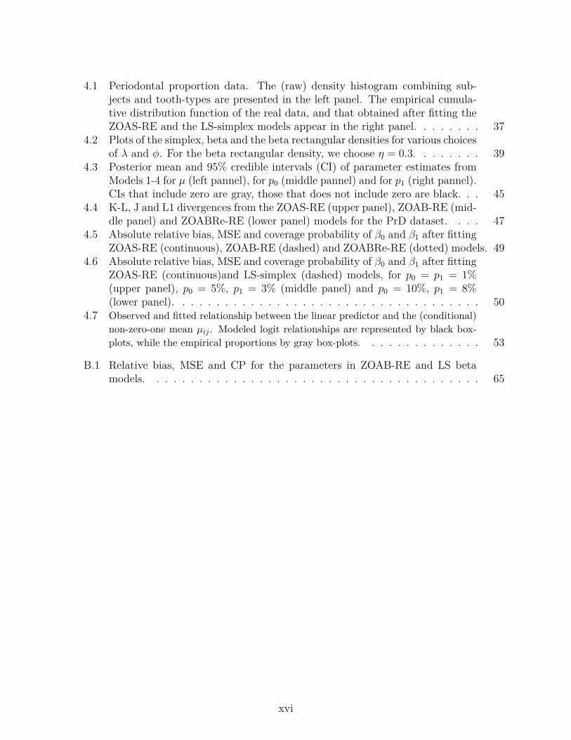
4.1 Periodontal proportion data. The (raw) density histogram combining sub-jects and tooth-types are presented in the left panel. The empirical cumula-tive distribution function of the real data, and that obtained after fitting theZOAS-RE and the LS-simplex models appear in the right panel. . . . . . . . 37

4.2 Plots of the simplex, beta and the beta rectangular densities for various choicesof ⁄ and „. For the beta rectangular density, we choose ÷ = 0.3. . . . . . . . 39

4.3 Posterior mean and 95% credible intervals (CI) of parameter estimates fromModels 1-4 for µ (left pannel), for p0 (middle pannel) and for p1 (right pannel).CIs that include zero are gray, those that does not include zero are black. . . 45

4.4 K-L, J and L1 divergences from the ZOAS-RE (upper panel), ZOAB-RE (mid-dle panel) and ZOABRe-RE (lower panel) models for the PrD dataset. . . . 47

4.5 Absolute relative bias, MSE and coverage probability of —0 and —1 after fittingZOAS-RE (continuous), ZOAB-RE (dashed) and ZOABRe-RE (dotted) models. 49

4.6 Absolute relative bias, MSE and coverage probability of —0 and —1 after fittingZOAS-RE (continuous)and LS-simplex (dashed) models, for p0 = p1 = 1%(upper panel), p0 = 5%, p1 = 3% (middle panel) and p0 = 10%, p1 = 8%(lower panel). . . . . . . . . . . . . . . . . . . . . . . . . . . . . . . . . . . . 50

4.7 Observed and fitted relationship between the linear predictor and the (conditional)non-zero-one mean µ

ij

. Modeled logit relationships are represented by black box-plots, while the empirical proportions by gray box-plots. . . . . . . . . . . . . . 53

B.1 Relative bias, MSE and CP for the parameters in ZOAB-RE and LS betamodels. . . . . . . . . . . . . . . . . . . . . . . . . . . . . . . . . . . . . . . 65

xvi

List of Tables

2.1 Model comparison using DIC3, LPML, EAIC and EBIC criteria. . . . . . . . . . 132.2 The values are the number of times higher/lower the ratio of the conditional

‘expected proportion of diseased sites’ (denoted by µij

) is, to the ‘expectedremaining proportion to complete disease’ (denoted by 1 - µ

ij

), conditional onthis proportion not being zero or one, with one unit increase in the covariates. 14

2.3 The values corresponding to p0ij represent odds of having a ‘disease free’ versus ‘diseased’ tooth-type, while

those for p1ij denote odds of ‘completely diseased’ versus ‘diseased and disease-free’ tooth types. . . . . 15

3.1 Posterior parameter (mean) estimates and standard deviations (SD) obtainedafter fitting Models 1-4 to the periodontal data. s denotes a significant pa-rameter. . . . . . . . . . . . . . . . . . . . . . . . . . . . . . . . . . . . . . . 30

4.1 Model comparison using DIC3, LPML, EAIC and EBIC criteria. . . . . . . . . . 454.2 Absolute Relative bias (Abs.RelBias), mean squared error (MSE), and cover-

age probabilities (CP) of the the parameter estimates after fitting the ZOAS-RE, ZOAB-RE, and ZOABRe-RE models to simulated data for various samplesizes. . . . . . . . . . . . . . . . . . . . . . . . . . . . . . . . . . . . . . . . . 54

B.1 Relative bias, MSE and CP for the parameters of ZOAB-RE and LS betamodels using di�erent sample size . . . . . . . . . . . . . . . . . . . . . . . . 64

C.1 Relative bias and MSE of the parameters in the ZOAS-RE and ZOAB-REmodels obtained with the prior – ≥ Gamma(1, 0.01) in the hiperparameterof Dirichlet distribution . . . . . . . . . . . . . . . . . . . . . . . . . . . . . 66

C.2 Relative bias and MSE of the parameters in the ZOAS-RE and ZOAB-REmodels obtained with the prior – ≥ Gamma(0.1, 0.01) in the hiperparameterof Dirichlet distribution. . . . . . . . . . . . . . . . . . . . . . . . . . . . . . 67

D.1 Results of the scheme of simulation 1 presented in the chapter 3 where thedata is analyzed of the ZOAS-RE model . . . . . . . . . . . . . . . . . . . . 68

D.2 Results of the scheme of simulation 1 presented in the chapter 3 where thedata analized by the ZOAS-RE model . . . . . . . . . . . . . . . . . . . . . . 68

xvii

xviii

Chapter 1

Introduction

Clinical studies often generate proportion data where the response of interest is continu-ous and confined in the interval (0, 1), such as percentages, proportions, fractions and rates(Kieschnick and McCullough, 2003). Examples include proportion of nucleotides that di�erfor a given sequence or gene in foot-and-mouth disease (Branscum et al., 2007), the percentdecrease in glomerular filtration rate at various follow-up times since baseline (Song and Tan,2000). Some of the strategies pointed out in the statistical literature to analyze this type ofdata are based on regression models combined with a particular data transformation suchas the logit transformation. However, the use of nonlinear transformations may hinder theinterpretation of the regression parameters. This situation can be overcome by consideringprobability distributions with double-bounded support, such as the beta, simplex (Barndor�-Nielsen and Jørgensen, 1991), and beta rectangular distributions (Hahn, 2008), which canbe parameterized in terms of their mean. Based on these models, regression models wereproposed.

The beta regression (BR) reparameterizes the associated beta parameters, connectingthe response to the data covariates through suitable link functions (Ferrari and Cribari-Neto, 2004). Yet, the beta density does not accommodate tail-area events, or flexibility invariance specifications (Bayes et al., 2012). To accommodate this, the BRe density Hahn(2008), and associated regression modelsBayes et al. (2012) were considered under a Bayesianframework. Note, the BRe regression includes the (constant dispersion) BRFerrari andCribari-Neto (2004), and the variable dispersion BRSmithson and Verkuilen (2006) as specialcases. The simplex regressionSong and Tan (2000) is based on the simplex distribution fromthe dispersion family (Jørgensen, 1997), assumes constant dispersion, and uses extendedgeneralized estimating equations for inference connecting the mean to the covariates via thelogit link. Subsequently, frameworks with heterogenous dispersion (Song et al., 2004), andfor mixed-e�ects models (Qiu et al., 2008) were explored. Yet, their potential were limitedto proportion responses with support in (0, 1).

The methodology developed in this thesis is motivated from a study conducted at theMedical University of South Carolina (MUSC) via a detailed questionnaire focusing on de-mographics, social, medical and dental history. In this study, was assessed the status andprogression of periodontal disease (PrD) among Gullah-speaking African-Americans withType-2 diabetes (Fernandes et al., 2006). The dataset contain measurements from ClinicalAttachment Level (CAL), obtained as the distance between the soft tissue in relation to

1

the cemento-enamel junction (see Figure 1.1), on six di�erent sites of each one of 28 teeth(considered full dentition, excluding the 4 third-molars). In this study were observed 290subjects, recording proportion of diseased tooth-sites. The proportion is calculated as thenumber of sites with the disease divided by the number of sites. This number depends onthe type of tooth, for example, there are 48 sites for molar, premolar and incisive, but 24sites for canine. A site is said to be diseased if the value of CAL is Ø 3mm. Hence, thisclustered data framework has 4 observations (corresponding to the 4 tooth-types) for eachsubject. If a tooth is missing, it was considered ‘missing due to PrD’, where all sites forthat tooth contributed to the diseased category. Note that in this case, the response lies inthe closed interval [0,1]; where 0 and 1 represent completely disease free and highly diseasedcases, respectively.

Subject-level covariables in the dataset include gender (0=male, 1= female), age of sub-ject at examination (in years, ranging from 26 to 87 years), glycosylated hemoglobin (HbA1c)status indicator (0=controlled,< 7%; 1=uncontrolled,Ø 7%) and smoking status (0=non-smoker,1=smoker). We also considered a tooth-level variable representing each of the fourtooth types, with ‘canine’ as the baseline.

Figure 1.1: Clinical attachment level.

The underlying statistical question here is to estimate the functions that model the depen-dence of the ‘proportion of diseased sites corresponding to a specific tooth-type (representedby incisors, canines, premolars and molars)’ with the covariables.

In this thesis are presented mixed regression models for proportional data in the presenceof zeros and ones as an alternative when the response is a vector with correlated compo-nents in [0, 1]. In this case, the estimation of the parameters, model selection and influencediagnostics follows a Bayesian approach.

2

1.1 Preliminaries1.1.1 Bayesian model selection and influence diagnosticsModel selection and assessments

There is a variety of methods for selecting the model that best fit a dataset. In thisthesis will be used the log pseudo-marginal likelihood (LPML), the observed informationcriterion DIC3, the expected Akaike information criterion (EAIC) and the expected Bayesianinformation criterion EBIC.

The LPML (Geisser and Eddy, 1979) is a summary statistic of the conditional pre-dictive ordinate (CPO) statistic and is defined by LPML =

nqi=1

log( [CPOi

), where [CPOi

can be obtained using a harmonic-mean approximation Dey et al. (1997) as [CPOi

=I1Q

Qqq=1

1f(yi|◊(q))

J≠1

and ◊(1), . . . , ◊(Q) is a post burn-in sample of size Q from the posterior

distribution of ◊ and f(yi

|◊(q)) is the marginal distribution of Y . Larger values of LPMLindicates better fit.

Some other measures, like the DIC, EAIC and EBIC Carlin and Louis (2008) can alsobe used. Because of the mixture framework in our models, we use the DIC3 Celeux et al.(2006) measure, which is an alternative to DIC Spiegelhalter et al. (2002). This is defined asDIC3 = D(◊) + ·

D

, D(◊) = ≠2E{log[f(y|◊)]|y}, f(y|◊) = rn

i=1 f(yi

|◊), E{log[f(y|◊)]|y}is the posterior expectation of log[f(y|◊)] and ·

D

is a measure of the e�ective number ofparameters in the model, given by ·

D

= D(◊) + 2 log(E[f(y|◊)|y]). Thus, we have DIC3 =≠4E{log[f(y|◊)]|y} + 2 log(E[f(y|◊)|y]). The first expectation in this expression can beapproximated by D = 1

Q

qQ

q=1q

n

i=1 logËf(y

i

|◊(q))È, as recommended by Celeux et al. (2006),

the second term in the expression can be approximated by qn

i=1 2 log f̂(yi

|◊) with f̂(yi

|◊) =1Q

qQ

q=1 f(yi

|◊(q)). The EAIC and EBIC can be estimated as \EAIC = ≠2D+2‹ and \EBIC =≠2D + ‹ log n, where ‹ is the number of parameters in the model, n is the number ofobservations and D defined above. Model selection follows the ‘lower is better’ law, i.e., themodel with the lowest value for these criteria gets selected.

Bayesian case influence diagnostics

In this section, we develop some influence diagnostics measures to study the impact ofoutliers on fixed e�ects parameter estimates motivated by data perturbation schemes basedon case-deletion statistics of Cook and Weisberg (1982). A common way of quantifyinginfluence with and without a given subset of data is to use the q-divergence measures Csiszet al. (1967); Weiss (1996) between posterior distributions. Consider a subset I with kelements from the whole dataset with n elements. When the subset I is deleted from thedata y, we denote the eliminated data as y

I

and the remaining data as y(≠I). Then, theperturbation function for deletion cases can be written as p(◊) = fi

1◊|y(≠I)

2/fi (◊|y). The q-

divergence measure between two arbitrary densities fi1 and fi2 for ◊ is defined as dq

(fi1, fi2) =s

q3

fi1(◊)fi2(◊)

4fi2(◊)d◊, where q is a convex function such that q(1) = 0. The q-influence of

3

the data yI

on the posterior distribution of ◊, dq

(I) = dq

(fi1, fi2), is obtained by consideringfi1(◊) = fi1(◊|y(≠I)) and fi2(◊) = fi(◊|y), and can be written as d

q

(I) = E◊|y {q(p(◊))}, wherethe expectation is taken with respect to the unperturbed posterior distribution. For variouschoices of the q(·) function, we have, for example, the Kullback-Leibler (KL) divergencewhen q(z) = ≠ log(z), the J-distance (symmetric version of the KL divergence) when q(z) =(z ≠ 1) log(z), and the L1-distance when q(z) = |z ≠ 1|.

Note that, dq

(I) defined above precludes itself from quantifying a cut-o� point beyondwhich an observation can be considered influential. Hence, we use the calibration methodPeng and Dey (1995), in that work, the q-divergence is given by d

q

(p) = q(2p)+q(2(1≠p))2 , where

dq

(p) increases as p moves away from 0.5, and is symmetric and reaches its minimum valueat 0.5. It is possible consider p Ø 0.90 (or p Æ 0.10), however, in this thesis will be usedp = 0.95. Thus, we can detect an influential observation (using the L1 distance) whend

L1(i) Ø 0.90, i = 1, . . . , n, for the KL divergence, we have dKL

(0.95) = 0.83, and for theJ-distance d

J

(0.95) = 1.32.

1.2 Organization of ThesisThis thesis is divided into five chapters and four appendices. The second chapter is an

already published paper and the fourth chapter is a paper that has been recently acceptedfor publication. In the fifth chapter are presented the conclusions and the plan for futureresearch. Next, I describe the results of chapters second to fourth.

• Chapter 2: Augmented mixed beta regression models for periodontal proportion data,published paper in Statistics in Medicine (2014).

– Description: In this chapter was proposed the Bayesian analysis of the zero andone augmented mixed beta regression (ZOAB-RE) model for clustered responsesin [0, 1], and applied it to an interesting PrD dataset. Through this model itwas possible to identifying covariates that are significant to explain disease-free,progressing with disease, and completely diseased tooth types. We also developedtools for outlier detection using q-divergence measures, and quantified their e�ecton the posterior estimates of the model parameters. Both simulation studiesand real data application justify seeking an appropriate theoretical model overutilizing ad hoc data transformations for proportion data

• Chapter 3: Augmented mixed models for clustered proportion data using the simplexdistribution.

– Description: In this chapter was proposed a Bayesian random e�ect model basedon the simplex distribution for modeling data in the interval [0, 1] called zero andone mixed simplex regression (ZOAS-RE) model. The versatility of this classto model correlated data in the interval [0, 1] has not been explored elsewhere,and this is our major contribution. Simulation studies reveal good consistencyproperties of the Bayesian estimates when compared with the ZOAS-RE regressioncounterpart, as well as, high performance of the model selection techniques to pickthe appropriately fitted model

4

• Chapter 4: Augmented mixed models for clustered proportion data. Accepted paperin Statistical Methods in Medical Research (2014).

– Description: In this chapter, it was proposed a class of (parametric) augmentedproportion distribution models. Particular cases of this family are the beta, betarectangular and simplex distributions. Based on this distributions were proposedthe regression models under a Bayesian framework, and demonstrate its applica-tion to the PrD dataset. Also, these regression models were compared using thePrD dataset and simulation studies. The results allow conclude that the ZOAS-RE model fits better to the PrD than the ZOAB-RE and zero and one augmentedbeta rectangular (ZOABr-RE) models. It was also concluded via simulation stud-ies.

5

Chapter 2

Augmented mixed beta regressionmodels for periodontal proportiondata

AbstractContinuous (clustered) proportion data often arise in various domains of medicine and pub-lic health where the response variable of interest is a proportion (or percentage) quantifyingdisease status for the cluster units, ranging between zero and one. However, due to the pres-ence of relatively disease-free as well as heavily diseased subjects in any study, the proportionvalues can lie in the interval [0, 1]. While Beta regression can be adapted to assess covariatee�ects in these situations, its versatility is often challenged due to the presence/excess of zerosand ones because the Beta support lies in the interval (0, 1). To circumvent this, we augmentthe probabilities of zero and one with the Beta density, controlling for the clustering e�ect.Our approach is Bayesian with the ability to borrow information across various stages of thecomplex model hierarchy, and produces a computationally convenient framework amenableto available freeware. The marginal likelihood is tractable, and can be used to developBayesian case-deletion influence diagnostics based on q-divergence measures. Both simula-tion studies and application to a real dataset from a clinical periodontology study quantifythe gain in model fit and parameter estimation over other ad hoc alternatives and providequantitative insight into assessing the true covariate e�ects on the proportion responses.

2.1 IntroductionClinical studies often generate proportion data where the response of interest is continu-

ous and confined in the interval (0, 1), such as percentages, proportions, fractions and rates(Kieschnick and McCullough, 2003). Examples include proportion of nucleotides that di�erfor a given sequence or gene in foot-and-mouth disease (Branscum et al., 2007), the percentdecrease in glomerular filtration rate at various follow-up times since baseline (Song and Tan,2000). With fidelity to the usual Gaussian assumptions for model errors, one might here betempted to fit a linear regression model to assess the response-covariate relationship (Qiuet al., 2008). However, this leads to misleading conclusions by ignoring the range constraints

6

in the responses. The logistic-normal model of Aitchison (1986), which assumes normaldistribution for logit-transformed proportion responses, can provide a computationally con-venient framework, but it su�ers from an interpretation problem given that the expectedvalue of response is not a simple logit function of the covariates. In this context, the betaregression (BR) proposed by Ferrari and Cribari-Neto (2004) can accomplish direct mod-eling of covariates under a generalized linear model (GLM) specification, leading to easyinterpretation. The beta density (Johnson et al., 1994) is extremely flexible, and can takeon a variety of shapes to account for non-normality and skewness in proportion data. TheBR model considers a specific re-parameterization of the associated beta density parameters,and connects the covariates with the mean and precision of the density through appropriatelink functions. Despite its versatility, its potential is limited for proportion responses withsupport in (0, 1).

The motivating data example for this paper comes from a clinical study (Fernandes et al.,2006), where the clinical attachment level (or, CAL), a clinical marker of periodontal disease(PrD), is measured at each of the 6 sites of a subject’s tooth. The underlying statisticalquestion here is to estimate the functions that model the dependence of the ‘proportionof diseased sites corresponding to a specific tooth-type (represented by incisors, canines,premolars and molars)’ with the covariables. Figure 1 (left panel) plots the raw (unadjusted)density histogram of the proportion responses aggregated over subjects and tooth types. Theresponses lie in the closed interval [0, 1] where 0 and 1 represent ‘completely disease free’,and ‘highly diseased’ cases, respectively. Although BR might be applicable here post (adhoc) re-scaling (Smithson and Verkuilen, 2006) of the data from [0, 1] to the interval (0, 1),various limitations are observed working on a transformed scale (Lachos et al., 2011). Thesere-scalings might provide a nice working solution for small proportions of 0’s and 1’s, butsensitivity towards parameter estimation can be considerable with higher proportions. Thisine�ciency is only aggravated due to the presence of additional clustering (tooth withinmouth/subject) in the data, as in our case. Hence, from a practical perspective, thereis a need to seek an appropriate theoretical model that avoids data transformations, yetis capable of handling the challenges the data present. To circumvent this, we propose ane�cient generalized linear mixed model (GLMM) framework by augmenting the probabilitiesof occurrence of zeros and ones to the BR model via a zero-and-one-augmented beta (ZOAB)random e�ects (ZOAB-RE) model, which can accommodate the subject-level clustering.

There have been various specifications of the BR model. The BR model of Ferrari andCribari-Neto (2004) re-parameterizes the beta density parameters and connects the datacovariates to the response mean via a logit link, assuming that the data precision is con-stant (nuisance) across all observations. This was subsequently modified by linking thecovariates to the dispersion parameter via the variable dispersion BR model by Smithsonand Verkuilen (2006). Very recently, Verkuilen and Smithson (2012) used Gauss-Hermitequadrature to calculate ML estimates and a Gibbs sampler for Bayesian estimation in thecontext of BR models for correlated proportion data. Also, Figueroa-Zúniga et al. (2013)presents a Bayesian approach to the correlated BR model through Gibbs samplers, and usesthe deviance information criterion (DIC) (Spiegelhalter et al., 2002), expected-AIC (EAIC)and expected-BIC (EBIC) for model selection. However, to the best of our knowledge, thereare no studies that utilize a Bayesian paradigm to model clustered (correlated) proportiondata where the proportions lie in the interval [0,1]. Our proposition ‘augments’ point masses

7

Proportion CAL data

Den

sity

0.0 0.2 0.4 0.6 0.8 1.0

0.00

0.02

0.04

0.06

0.08

0.10

0.12

0.0 0.1 0.2 0.3 0.4 0.5 0.6 0.7 0.8 0.9 1.0

0.0

0.1

0.2

0.3

0.4

0.5

0.6

0.7

0.8

0.9

1.0

Proportion CAL data

Cum

ulat

ive p

erce

nt

Actual DataZOAB−RE ModelLS Model

Figure 2.1: The left panel plots the (raw) density histogram, aggregated over subjects andtooth-types for the PrD data. The ‘pins’ at the extremes represent the proportion of zeros(9.8%) and ones (8.1%). The right panel presents the empirical cumulative distributionfunction of the real data, and that obtained after fitting the ZOAB-RE (Model 1) and theLS model (Model 3).

at zero and one to a continuous (beta) density that does not include zero and one in itssupport, similar in spirit to Hatfield et al. (2012). In addition, following the pioneering workof Cook (1986), we develop case-deletion and local influence diagnostics to assess the e�ectof outliers on the parameter estimates. Our approach is Bayesian, with the ability to borrowinformation across various stages of the complex model hierarchy, and produces a computa-tionally convenient framework amenable to available freeware like OpenBUGS (Thomas et al.,2006).

The rest of the article proceeds as follows. After a brief introduction to the BR model,Section 2 introduces the ZOAB-RE model, and develops the Bayesian estimation scheme.Section 3 applies the proposed ZOAB-RE model to the motivating data and uses Bayesianmodel selection to select the best model. It also summarizes and discusses the estimationof the fixed e�ects, other model parameters and outlier detections. Section 4 presents sim-ulation studies to assess finite sample performance of our model with another competingtransformation-based model under model misspecification, and also to study the e�ciencyof the influence diagnostic measures to detect outliers. Conclusions and future developmentsappear in Section 6.

8

2.2 Statistical Model and Bayesian Inference2.2.1 Beta regression model

The beta distribution is often the model of choice for fitting continuous data restrictedin the interval (0,1) due to the flexibility it provides in terms of the variety of shapes it canaccommodate. The probability density function of a beta distributed random variable Yparameterized in terms of its mean µ and a precision parameter „ is given by

f(y|µ, „) = �(„)�(µ„)�((1 ≠ µ)„)yµ„≠1(1 ≠ y)(1≠µ)„≠1, 0 < y < 1, 0 < µ < 1, „ > 0, (2.2.1)

where �(·) denotes the gamma function, E(Y ) = µ, and Var(Y ) = µ(1 ≠ µ)1 + „

. Therefore, fora fixed value of the mean µ, higher values of „ leads to a reduction of Var(Y ), and conversely.If Y has pdf as in (2.2.1), we write Y ≥ beta(µ„; (1 ≠ µ)„). Next, to connect the covariatevector x

i

to the random sample Y1, . . . , Yn

of Y , we use a suitable link function g1 that mapsthe mean interval (0,1) onto the real line. This is given as g1(µi

) = x€i

—, where — is thevector of regression parameters, and the first element of x

i

is 1 to accommodate the intercept.The precision parameter „

i

is either assumed constant (Ferrari and Cribari-Neto, 2004), orregressed onto the covariates (Smithson and Verkuilen, 2006) via another link function h1,such that h1(„i

) = zT

i

–, where zi

is a covariate vector (not necessarily similar to xi

), and– is the corresponding vector of regression parameters. Similar to x

i

, zi

also accommodatesan intercept. Both g1 and h1 are strictly monotonic and twice di�erentiable. Choices ofg1 includes the logit specification g1(µi

) = log{µi

/(1 ≠ µi

)}, the probit function g1(µi

) =�≠1(µ

i

) where �(·) is the standard normal density, the complementary log-log functiong1(µi

) = log{≠log(1 ≠ µi

)} among others, and for h1, the log function h1(„i

) = log(„),the square-root function h1(„i

) =Ô

„i

, and the identity function h1(„i

) = „i

(with specialattention to the positivity of the estimates) (Simas et al., 2010). Estimation follows via eitherthe (classical) maximum likelihood (ML) route (Ferrari and Cribari-Neto, 2004) or throughGauss-Hermite quadratures (Smithson and Verkuilen, 2006) available in the betareg libraryin R (Zeileis et al., 2010), or Bayesian (Branscum et al., 2007) through Gibbs sampling.

2.2.2 Zero-and-one augmented beta random e�ects modelThe BR model described above only applies to observations that are independent, and

moreover it is suitable only for responses lying in (0, 1). However, for our PrD dataset,the responses pertaining to a particular subject are clustered in nature, and lie boundedin [0, 1]. We now develop a ZOAB model to address both the bounded support problemand the data clustering. Our proposition comprises a three-part mixture distribution, withdegenerate point masses at 0 and 1, and a beta density to have the support of Y

i

œ [0, 1].Thus, Y ≥ ZOAB(p0

i

, p1i

, µi

, „), if the density of Yi

, i = 1, . . . , n, follows

f(yi

|p0i

, p1i

, µi

, „) =

Y_]

_[

p0i

if yi

= 0,p1

i

if yi

= 1,(1 ≠ p0

i

≠ p1i

)f(yi

|µi

, „) if yi

œ (0, 1),(2.2.2)

9

where p0i

Ø 0 denotes P (Yi

= 0), p1i

Ø 0 denotes P (Yi

= 1), 0 Æ p0i

+p1i

Æ 1 and f(yi

|µi

, „)is given in (2.2.1). The mean and variance of Y

i

are given by

E[Yi

] = (1 ≠ p0i

≠ p1i

)µi

+ p1i

and

Var(Yi

) = p1i

(1 ≠ p1i

) + (1 ≠ p0i

≠ p1i

)C

µi

(1 ≠ µi

)1 + „

+ (p0i

+ p1i

)µ2i

≠ 2µi

p1i

D

.

For clustered data, the ZOAB-RE model is defined as follows. Let Y1, . . . , Yn

be nindependent continuous random vectors, where Y

i

= (yi1, . . . , y

ini) is the vector of length ni

for the sample unit i, with the components yij

œ [0, 1]. Next, the covariates can be regressedonto a suitably transformed µ

ij

, p0ij

and p1ij

, such that

g1(E[Yi

|bi

]) = g1(µi

) = X€i

— + Z€i

bi

, (2.2.3)g2(p0

i

) = W0€i

Â, (2.2.4)g3(p1

i

) = W1€i

fl, (2.2.5)

where µi

= (µi1, . . . , µ

ini), p0i

= (p0i1, . . . , p0

ini), p1

i

= (p1i1, . . . , p1

ini); X

i

, W0i

and W1i

are design matrices of dimension p◊ni

, r◊ni

and s◊ni

, corresponding to the vectors of fixede�ects — = (—1, . . . , —

p

)€, Â = (Â1, . . . , Âr

)€, fl = (fl1, . . . , fls

)€, respectively, and Zi

is thedesign matrix of dimension q ◊ n

i

corresponding to REs vector bi

= (bi1, . . . , b

iq

)€. Choiceof link functions for g1, g2 and g3 here remain the same as for g1 in Subsection 2.2.1. For thesake of interpretation, we prefer to use the logit link. Note that in our model development,the dispersion parameter „ is chosen as constant and the regressions onto p0

i

and p1i

arefree of REs to avoid over-parameterization. However, it is certainly possible to regress „onto covariates through an appropriate link function (say, log). Also, p0ij

and p1ij

can betreated as constants across all sample units. To this end, we define our ZOAB-RE model asY

ij

≥ ZOAB-RE(p0ij

, p1ij

, µij

, „) i = 1, . . . , n, j = 1, . . . , ni

.

2.2.3 Likelihood functionLet � = (—, Â, fl, „) denote the parameter vector in this ZOAB-RE model. The primary

goal here is to estimate �, and to derive inference on — adjusting for the e�ects of clustering.Our observed sample for n subjects is (y1, X1, Z1, W01, W11), . . . , (y

n

, Xn

, Zn

, W0n

, W1n

),with y

i

as the response vector for subject i. The joint data likelihood (without integratingout the random-e�ects b

i

) is given as:

L(�|b, y, X, Z, W0, W1) =nŸ

i=1L

i

(�|bi

, yi

, Xi

, Zi

, W0i

, W1i

), (2.2.6)

where

Li

(�|bi

, yi

, Xi

, Zi

, W0i

, W1i

) = §Ëp0

€i

D0i

+ p1€i

D1i

+ (1 ≠ p0i

≠ p1i

)€(Ini ≠ D0

i

≠ D1i

)Bi

È€,

§Ai

indicates the product of the elements of Ai

, p0i

= (p0i1, . . . , p0

ini)€ with p0

ij

=exp(W0

€ij

Â)1 + exp(W0

€ij

Â), p1

i

= (p1i1, . . . , p1

ini)€, with p1

ij

=exp(W1

€ij

fl)1 + exp(W1

€ij

fl), D

k

i

is a diagonal

10

matrix of dimension ni

◊ ni

whose j-th element of the diagonal is the indicator func-tion I{yij=k}, k = 0, 1, j = 1, . . . , n

i

, Ini is the identity matrix with dimension n

i

◊ ni

and Bi

is a diagonal matrix of dimension ni

◊ ni

whose j-th element of the diagonal is�(„)

�(µij„)�((1≠µij)„)yµij„≠1ij

(1 ≠ yij

)(1≠µij)„≠1 and µij

=exp(X€

ij

— + Z€ij

bi

)1 + exp(X€

ij

— + Z€ij

bi

) , Xij

and Zij

cor-

respond to the j-th column of the matrices Xi

and Zi

, respectively.Although one can certainly pursue a classical estimation route using maximum likeli-

hood methods following Ospina and Ferrari (2010), a Bayesian treatment of our model hasnot been considered earlier in the literature. Recent developments in Markov chain MonteCarlo (MCMC) methods facilitate easy and straightforward implementation of the Bayesianparadigm through conventional software such as OpenBUGS. Hence, we consider a Bayesianestimation framework which can accommodate full parameter uncertainty through appropri-ate prior choices supported by proper sensitivity investigations. This framework can providea direct probability statement about a parameter through credible intervals (C.I.) (Dun-son, 2001). Next, we investigate the choice of priors for our model parameters to conductBayesian inference.

2.2.4 Prior and posterior distributionsWe specify practical weakly informative prior opinion on the fixed e�ects regression pa-

rameters —, Â, fl, „ (dispersion parameter) and the random e�ects bi

. Specifically, weassign i.i.d Normal(0, precision = 0.01) priors on the elements of —, Â and fl, which cen-ters the ‘odds-ratio’ type inference at 1 with a su�ciently wide 95% interval. Priors for„ ≥ Gamma(0.1, 0.01), and b

i

are Normal with zero mean and precision = 1/‡2b

), where‡

b

≥ Unif(0, 100) (Gelman, 2006). Although multivariate specifications (multivariate zeromean vector with inverted-Wishart covariance) are certainly possible, we stick to simple (andindependent) choices. For cases where p0 and p1 are considered constants across all subjects,we allocate the Dirichlet prior with hyperparameter – = (–1, –2, –3) for the probabilityvector (p0, p1, 1 ≠ p0 ≠ p1), where –

s

≥ Gamma(1, 0.001), s = 1, 2, 3.The posterior conclusions are based on the joint posterior distribution of all the model

parameters (conditional on the data), and obtained by combining the likelihood given in(2.2.6), and the joint prior densities using the Bayes’ Theorem:

p(◊, b|y, X, Z, W0, W1) Ã L(�|b, y, X, Z, W0, W1)◊fi0(—)◊fi1(Â)◊fi2(fl)◊fi3(„)◊fi4(b|‡b

)◊fi5(‡b

),(2.2.7)

where ◊ = (�, ‡2b

)€, fij

(.), j = 0, . . . , 5 denote the prior/hyperprior distributions on themodel parameters as described above. The relevant MCMC steps (combination of Gibbs andMetropolis-within-Gibbs sampling) was implemented using the BRugs package (Ligges et al.,2009) which connects the R language with the OpenBUGS software. After discarding 50000burn-in samples, we used 50000 more samples (with spacing of 10) from two independentchains with widely dispersed starting values for posterior summaries. Convergence wasmonitored via MCMC chain histories, autocorrelation and crosscorrelation, density plots,and the Brooks-Gelman-Rubin potential scale reduction factor R̂, all available in the R codalibrary (Cowles and Carlin, 1996). Associated BRugs code is available on request from thecorresponding author.

11

2.2.5 Bayesian model selection and influence diagnosticsWe use the conditional predictive ordinate (CPO) statistic (Carlin and Louis, 2008) for

our model selection derived from the posterior predictive distribution (ppd). A summarystatistic obtained from the CPO is the log pseudo-marginal likelihood (LPML) (Carlin andLouis, 2008). Larger values of LPML indicate better fit. Because the harmonic-mean iden-tity used in the CPO computation can be unstable (Raftery et al., 2007), we consider amore pragmatic route and compute the CPO (and associated LPML) statistics using 500non-overlapping blocks of the Markov chain, each of size 2000 post-convergence (i.e., afterdiscarding the initial burn-in samples), and report the expected LPML computed over the500 blocks. Some other measures, like the deviance information criteria (DIC), expectedAIC (EAIC) and expected BIC (EBIC) (Carlin and Louis, 2008) can also be used. Becauseof the mixture framework in our ZOAB-RE model, we use the DIC3 (Celeux et al., 2006)measure as an alternative to the DIC (Spiegelhalter et al., 2002). Model selection followsthe ‘lower is better’ law, i.e., the model with the lowest value for these criteria gets selected.

To determine model adequacy after selecting the best model, we apply the Bayesian p-value (Gelman et al., 2004) which utilizes some discrepancy measures based on ppd. Samplesfrom the ppd (denoted by y

pr

) are replicates of the observed model generated data y, hencethere is some signal of model inadequacy if the observed value is extreme relative to thereference ppd. Because of the clustered nature of our data, we consider the sum statisticT (y, ◊) = sum(y) as our discrepancy measure. Then, the Bayesian p-value p

B

is calculatedas the number of times T (y

pr

, ◊) exceeds T (y, ◊) out of L simulated draws, i.e., pB

=Pr(T (y

pr

, ◊) Ø T (y, ◊)|y). A very large p-value (> 0.95), or a very small one (< 0.05)signals model misspecification.

In addition, some influence diagnostic measures are developed to study the impact ofoutliers on fixed e�ects parameter estimates caused by data perturbation schemes based oncase-deletion statistics (Cook and Weisberg, 1982), and the q-divergence measures (Csiszet al., 1967; Weiss, 1996; Lachos et al., 2013) between posterior distributions. We use threechoices of these divergences, namely, the Kullback-Leibler (KL) divergence, the J-distance(symmetric version of the KL divergence), and the L1-distance. We use the calibrationmethod (Peng and Dey, 1995) to obtain the cut-o� values as 0.90, 0.83 and 1.32 for the L1,KL and J-distances, respectively.

2.3 Data analysis and findingsIn this section, we apply our proposed ZOAB-RE model to the PrD data. We start with

a short description of the dataset. A study assessing the status and progression of PrDamong Gullah-speaking African-Americans with Type-2 diabetes (Fernandes et al., 2006)was conducted at the Medical University of South Carolina (MUSC) via a detailed ques-tionnaire focusing on demographics, social, medical and dental history. CAL was recordedat each of the 6 tooth-sites per tooth for 28 teeth (considered full dentition, excluding the4 third-molars). With 290 subjects, we focus on quantifying the extent and severity of PrDfor the tooth-types (4 canines and 8 each of incisors, pre-molars and molars). Our responsevariable is: ‘Proportion of diseased tooth-sites (with CAL value Ø 3mm) for each of the four

12

tooth types’. This gives rise to a clustered data framework where each subject records 4observations corresponding to the 4 tooth-types. Missing teeth were considered ‘missing dueto PrD’, where all sites for that tooth contributed to the diseased category. Subject-levelcovariables in this dataset include gender (0=male,1= female), age of subject at examination(in years, ranging from 26 to 87 years), glycosylated hemoglobin (HbA1c) status indicator(0=controlled,< 7%; 1=uncontrolled,Ø 7%) and smoking status (0=non-smoker,1=smoker).The smoker category is comprised of both the current and past smokers. We also considereda tooth-level variable representing each of the four tooth types, with ‘canine’ as the baseline.As observed in the density histogram in Figure 2.1 (Panel left), the data are continuous in therange [0,1]. Due to the presence of a substantial number of 0’s (114, 9.8%) and 1’s (94, 8.1%),BR might be inappropriate here. Hence, we resort to the ZOAB-RE model, controlling forsubject-level clustering. From Equation (2.2.3), we now have ÷

i

= g1(µi

) = X€i

— + bi

, with

ModelCriterion 1 2

DIC3 993.0 1243.5LPML ≠500.5 -623.7EAIC 992.7 1231.0EBIC 1124.2 1286.6

Table 2.1: Model comparison using DIC3, LPML, EAIC and EBIC criteria.

g1 the logit link, —€ = (—0, . . . , —7), with —0 the intercept and —1, . . . , —7 the regression pa-rameters, X€

i

= (1, Genderi

, Agei

, HbA1ci

, Smokeri

, Incisori

, Premolari

, Molari

), and bi

is thesubject-level random e�ect term. To improve convergence of the sampler, we standardized‘Age’ by subtracting its mean and dividing by its standard deviation. Note that, here themodel covariates are regressed onto µ

ij

, p0ij

and p1ij

, but it is also possible to consider p0and p1 constants across all subjects. This leads to our choice of two competing models:

Model 1: logit(µi

) = ÷i

, logit(p0i

) = W0€i

 and logit(p1i

) = W0€i

fl, with W0€i

=W1

€i

= X€i

.Model 2: logit(µ

i

) = ÷i

p0i

= p0 and p1i

= p1.

We also fit a non-augmented BR model by transforming the data points y to yÕ viathe lemon-squeezer (LS) transformation given by yÕ = [y(N ≠ 1) + 1/2]/N (Smithson andVerkuilen, 2006), where N is the total number of observations, and fit the above regressionsto µ

i

with the logit link. This is our Model 3, or the LS model. Although other linkfunctions (such as probit, cloglog, etc) are available, we currently restrict ourselves to thesymmetric logit link whose adequacy is assessed later. Note that Models 1 and 2 which fit thesame dataset can be compared using the model choice criteria described in Subsection 2.2.5,but not Model 3 since it considers a transformed dataset. Hence, Model 3 is assessed usingplots of empirical cumulative distribution functions (ecdfs) of the fitted values to determinehow closely the fits resemble the true data.

13

Molar

Premolar

Incisor

Smoker

HbA1c

Age

Gender

Intercept

−1 0 1 2 3

Model 1Model 2Model 3

Figure 2.2: Posterior mean and 95% CIs of pa-rameter estimates from Models 1-3. CIs thatinclude zero are gray, those that does not in-clude zero are black.

Table 2.2: The values are the number of timeshigher/lower the ratio of the conditional ‘ex-pected proportion of diseased sites’ (denotedby µ

ij

) is, to the ‘expected remaining propor-tion to complete disease’ (denoted by 1 - µ

ij

),conditional on this proportion not being zeroor one, with one unit increase in the covari-ates.

Parameter Model 1 Model 2 Model 3Intercept 0.5 0.5 0.4Gender 0.6 0.6 0.5

Age 1.4 1.4 1.6HbA1c 1.1 1.1 1.3Smoker 1.1 1.1 1.0Incisor 1.2 1.2 1.4

Premolar 2.3 2.3 3.1Molar 8.5 8.5 15.3

In the absence of historical data/experiment, our prior choices follow the specificationsdescribed in Section 2.2.4. Table 2.1 presents the DIC3, LPML, EAIC and EBIC valuescalculated for Models 1 and 2. Notice that Model 1 (our ZOAB-RE model with regressionon µ

ij

, p0ij

and p1ij

) outperforms Model 2 for all criteria. From Figure 2.1 (right panel),it is also clear that the ecdf from the fitted values using Model 1 represent the true datamore closely than Model 3. Considering these, we select Model 1 as our best model. Withrespect to goodness-of-fit assessment, p

B

= 0.798, which indicates no overall lack of fit.Figure 2.2 plots the posterior parameter means and the 95% credible intervals (CIs) for theregression onto µ for Models 1-3. The gray intervals in Figure 2.2 contain zero (the non-significant covariates), while the black intervals do not include zero (the significant ones at5% level). The covariates gender, age, and the tooth types (incisor, premolar and molar)significantly explain the proportion responses. Conditional on the set of other covariatesand REs, parameter interpretation can be expressed in terms of the corresponding covariatee�ect directly on µ

ij

, specifically the ratio µij

1≠µij. Here, µ

ij

is the ‘expected proportion ofdiseased sites’, and 1 ≠ µ

ij

is the complement, i.e., the ‘expected remaining proportion tobeing completely diseased’, both conditional on Y

ij

not being zero or one. Hence, the resultsin Table 2.2 can be expressed as the number of times the ratio is higher/lower with everyunit increase (for a continuous covariate, such as age), or a change in category say from 0 to1 (for a discrete covariate, say gender). For example, this ratio for age (a strong predictorof PrD) is (1.4, 95%CI = [1.2, 1.6]). For gender, we conclude that this ratio is 40% lower formales as compared to females. Although study recruitment design was gender blind, females

14

Molar

Premolar

Incisor

Smoker

HbA1c

Age

Gender

Intercept

−8 −6 −4 −2 0 2 −4 −2 0 2

Figure 2.3: Posterior mean and 95% CI of parameter estimatesfor p0ij

(left panel) and p1ij

(right panel) from Model 1. CIsthat include zero are gray, those that does not include zero areblack.

Table 2.3: The values correspond-ing to p0ij represent odds of havinga ‘disease free’ versus ‘diseased’ tooth-type, while those for p1ij denote oddsof ‘completely diseased’ versus ‘diseasedand disease-free’ tooth types.

Parameter p0ij

p1ij

Intercept 0.2 0.03Gender 2.9 0.5

Age 0.6 2.5HbA1c 0.7 1.4Smoker 0.7 0.7Incisor 0.5 1.4

Premolar 0.08 1.3Molar 0.005 13.3

participated at a higher rate than the males, not unusual for studies on this population(Johnson-Spruill et al., 2009; Bandyopadhyay et al., 2009), and further patient navigatortechniques are being developed to achieve better gender balance. The other significantcovariates can be interpreted similarly. For example, this ratio is 8.5 times higher for theposteriorly located molars as compared to anteriorly placed canines (the baseline).

The mean estimates (standard deviations) of „ for the Models 1, 2 and 3 are 7.6 (0.42),7.6 (0.43) and 4.6 (0.26), and those of ‡2

b

are 1.2 (0.13), 1.2 (0.13) and 1.8 (0.18), respectively.Based on these and from Table 2.2, we conclude there is little di�erence between the Models1 and 2 with respect to the estimates of —, „ and ‡2

b

. The main advantage of Model 1is that it identifies significant covariates related to free PrD and completely diseased toothtypes, which is not available in Model 2. However, the estimates of premolar, molar, „ and‡2

b

obtained from Model 3 are greater than those obtained from Models 1 and 2, with thehighest di�erence being for molar. Interestingly, the estimates of „ (‡2

b

) from Model 3 aresmaller (greater) than those from Models 1 and 2, implying that augmenting leads to a lower(estimated) variance of Y than the transformation-based Model 3.

Figure 2.3 plots the posterior parameter means and the 95% CIs of the parametersused to model p0 (left panel) and p1 (right panel) for Model 1. Gender, age and type oftooth significantly explain free of PrD, while gender, age and molar significantly explain thecompletely diseased category. Table 2.3 presents the number of times higher/lower of theodds for free of PrD (second column) and completely diseased (third column). For example,the odds of a tooth type free of PrD are 2.9 times greater for men than for women, whilethe odds of a completely diseased molar are about 13 times that that of a (baseline) Canine.Interestingly, the odds of a completely diseased tooth type are 2.5 times higher for a unit

15

−1.6 −1.3 −0.9 −0.6 −0.2 0.1 0.5 0.9 1.4 3.4

0.0

0.2

0.4

0.6

0.8

1.0

Linear predictor (deciles)

E[Y|

Y≠

0,1]

−1.6 −1.3 −0.9 −0.6 −0.2 0.1 0.5 0.9 1.4 3.4

0.0

0.2

0.4

0.6

0.8

1.0

Figure 2.4: Observed and fitted relationship between the linear predictor ÷ij

and the (con-ditional) non-zero-one mean µ

ij

. Modeled logit relationships are represented by black box-plots, while the empirical proportions by gray box-plots.

increase in age. Interpretation for the other parameters is similar.To investigate the adequacy of the logit link for our regression, we consider an empirical

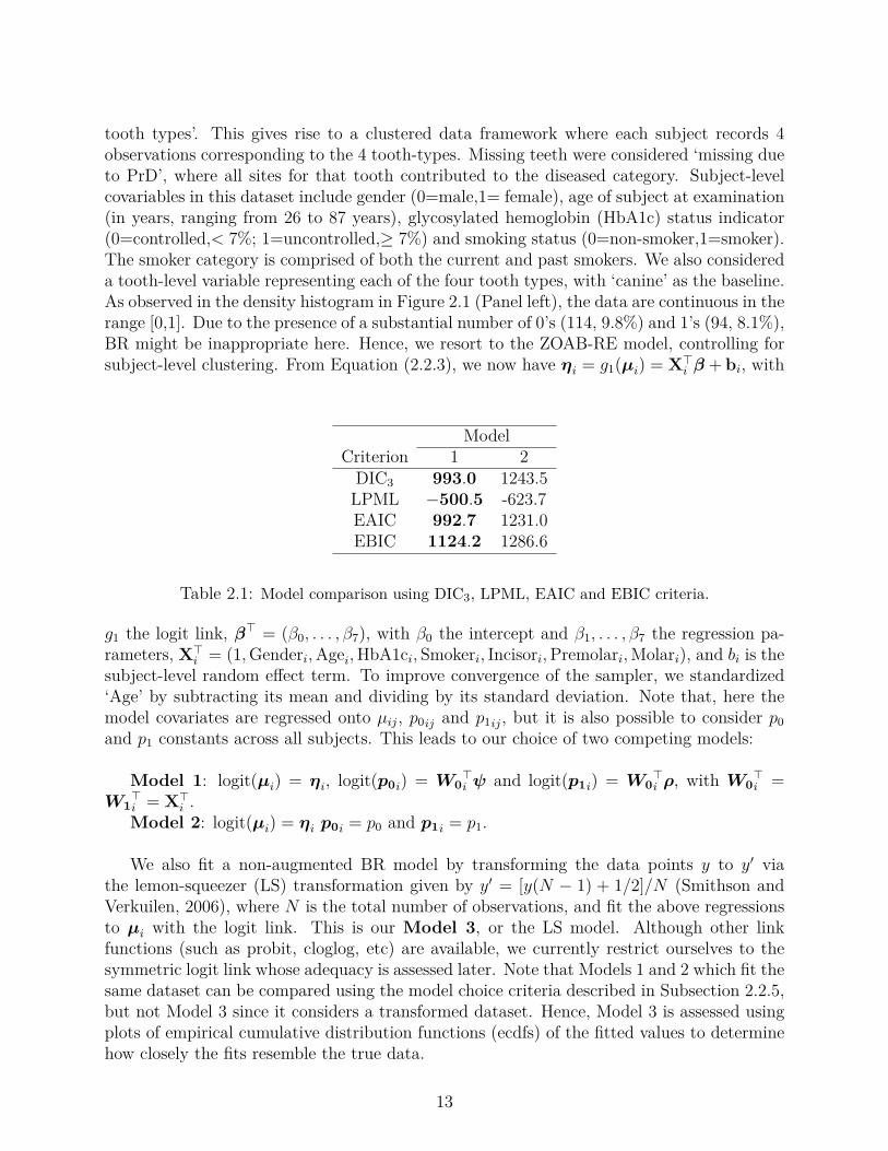
approach via plots of the linear predictor versus the predicted probability (Hatfield et al.,2012), as depicted in Figure 2.4. We consider ÷

ij

from Model 1, and divide it into 10 intervalscontaining roughly an equal number of observations. We plot the distribution of the inverse-logit transformed linear predictors (denoted by the black box-plots) representing the fittedmean µ

ij

of the non-zero-one responses. Next, we overlay the empirical distributions ofthe observed non-zero-one responses represented by the gray box-plots. From Figure 2.4,we observe no evidence of link misspecification, i.e., the shapes of the fitted and observedtrends are similar. As mentioned earlier, one can definitely fit other link functions, but theconvenient interpretations in terms of µ

ij

are no longer valid for these fits.We also conducted a sensitivity analysis on the prior assumptions for the random ef-

fects precision (1/‡2b

) and the fixed e�ects precision parameter. In particular, we allowed‡

b

≥ Uniform(0, k), where k œ {10, 50} and also the typical Inverse-gamma choice for theprecision 1/‡2

b

≥ Gamma(k, k), where k œ {0.001, 0.1}. We also chose the normal precisionon the fixed e�ects to be 0.1, 0.25 (which reflects an odds-ratio in between e≠4 to e4) and0.001. We checked the sensitivity in the posterior estimates of — by changing one parameterat a time, and refitting Model 1. Although slight changes were observed in parameter esti-mates and model comparison values, the results appeared to be robust, and did not changeour conclusions regarding the best model, inference (and sign) of the fixed-e�ects, and theinfluential observations.

Finally, to determine the e�ect of possible influential observations, we computed the q-

16

divergence measures for Model 1. In particular, the subjects with id # 135, 159, 174 and285 were considered influential because the values of the L1, KL and J-distances exceededthe specified thresholds. The subjects 135, 159 and 285 have higher proportion responsesfor all tooth types (with Y

ij

Ø 0.75) for than the corresponding mean proportions across allsubjects. On the contrary, subject 174 is free of PrD (Y

ij

= 0) across all tooth types. Toquantify the impact of these observations on the covariate e�ects, we refit the model by firstremoving these subjects successively, and then as a whole. Compared to other covariates, theestimate of molar for the regression onto p0ij

was impacted substantially. A minor impacton smoker for regression onto p0ij

was also observed when all influential observations wereremoved. Overall, parameter significance and signs of the coe�cients remained the same.Henceforth, we assert to use the estimates obtained from fitting Model 1 to the full datawithout removing these subjects.

2.4 Simulation studiesIn this section, we conduct two simulation studies. For the first, we plan to investigate

the consequences on the (regression) parameter estimation under model misspecification viamean squared error (MSE), relative bias (RB), and coverage probability for the (a) ZOAB-RE model (Model 1), and (b) the LS model (Model 3) for varying sample sizes. In the second,we evaluate the e�ciency of the q-divergence measures to detect atypical observations in theZOAB-RE model.

Simulation 1: We generate Tij

≥ Normal(µij

, 1), where i = 1, . . . , n (the number ofsubjects), j = 1, . . . , 5 (indicating cluster of size 5 for each subject), with location parameterµ

ij

modeled as µij

= —0 + —1xij

+ bi

, and bi

≥ N(0, ‡2). Then, yij

= exp(Tij)1+exp(Tij) . We choose

various sample sizes n = 50, 100, 150, 200. The explanatory variables xij

are generated asindependent draws from a Uniform(0, 1), and regression parameters and variance componentsare fixed at —0 = ≠0.5, —1 = 0.5, and ‡2 = 2. This generates data from a logit-normal modelwith y

ij

œ (0, 1). Next, we can have two sets of p0 and p1; namely, Case (a): p0 = 0.01, p1 =0.01 and Case (b): p0 = 0.1, p1 = 0.08 (representative of the real data). The final step is toallocate the 0’s, 1’s, and the y

ij

œ (0, 1) with probabilities p0, p1 and 1 ≠ p0 ≠ p1, which isachieved via multinomial sampling. To keep the simulation design simple, we do not considerthe regressions onto p0 and p1.

In the first simulation study, we simulated 500 such data sets and fitted the ZOAB-RE and the LS models with similar prior choices as in the data analysis. With our pa-rameter vector ◊ = (—0, —1, ‡2

b

, p0, p1), and ◊s

an element of ◊, we calculate the MSE asMSE(◊̂

s

) = 1500

q500i=1(◊̂is

≠ ◊s

)2, the relative bias as Relative Bias(◊̂s

) = 1500

q500i=1

1◊̂is◊s

≠ 12,

and the 95% coverage probability (CP) as CP(◊̂s

) = 1500

q500i=1 I(◊

s

œ [◊̂s,LCL

, ◊̂s,UCL

]), whereI is the indicator function such that ◊

s

lies in the interval [◊̂s,LCL

, ◊̂s,UCL

], with ◊̂s,LCL

and◊̂

s,UCL

as the estimated lower and upper 95% limitis of the CIs, respectively. Figure 2.5presents a visual comparison of the parameters —0 and —1 for varying sample sizes and pro-portions p0 and p1, where the black and gray lines represent the ZOAB-RE model and theLS model, respectively.

As expected, both panels of Figure 2.5 reveal that the absolute values of RB for both —0

17

50 150

−1.2

−0.8

−0.4

0.00.2

n

Relat

ive bi

as

β0

p0=1%p1=1%

50 150

0.00

0.05

0.10

0.15

0.20

n

MSE

50 150

0.00.2

0.40.6

0.81.0

nCP

ZOAB−RELS

50 150

−1.2

−0.8

−0.4

0.00.2

n

Relat

ive bi

as

β1

50 150

0.00

0.05

0.10

0.15

0.20

n

MSE

50 150

0.00.2

0.40.6

0.81.0

n

CP

50 150

−1.2

−0.8

−0.4

0.00.2

n

Relat

ive bi

as

β0

p0=10%p1=8%

50 150

0.00

0.05

0.10

0.15

0.20

n

MSE

50 150

0.00.2

0.40.6

0.81.0

1.2

n

CP

50 150

−1.2

−0.8

−0.4

0.00.2

n

Relat

ive bi

as

β1

50 1500.0

00.0

50.1

00.1

50.2

0

n

MSE50 150

0.00.2

0.40.6

0.81.0

1.2

n

CP

Figure 2.5: Relative Bias, MSE and CP of —0 and —1 after fitting the ZOAB-RE (black line)and LS (gray line) models, with p0 = p1 = 1% (upper panel) and p0 = 10%,p1 = 8% (lowerpanel).

and —1 are much larger for the LS model than the ZOAB-RE model, with the RB increasingwith increasing p0 and p1 (Case b). We observe similar behavior for MSE and CP, i.e., boththe parameters from the ZOAB-RE model are estimated with lower MSE and higher CPwhen compared to the corresponding ones from the LS model, with the performance of theLS model getting worse with increasing proportions of extreme values. Clearly, when dataare generated from a misspecified (augmented logit-normal) model, the LS model seems toproduce a considerable impact on the regression parameter estimates as compared to themore robust ZOAB-RE model. For the sake of brevity, the MSE, RB and CP for the otherparameters (p0, p1, ‡2

b

) are not presented here, but we discuss the results. The proportionsp0 and p1 are estimated with positive RB. Interestingly, for ‡2

b

, the RB remains negative forall cases, with the absolute value of the RB increasing with increasing sample size mainlyfor the LS model. This might occur because the LS transformation induces lower variabilityin the data leading to an underestimated ‡2

b

and RB. With this increase in RB, the 95% CIdoes not include the true value of ‡2

b

, and hence the CP is mostly 0 for higher n (150 and200) for both models in Case (a), and also for all sample sizes for the LS model in Case (b).We conclude that under model misspecification, applying the LS transformation may notbe adequate even for a moderate number of 0’s and 1’s, with the performance deteriorating

18

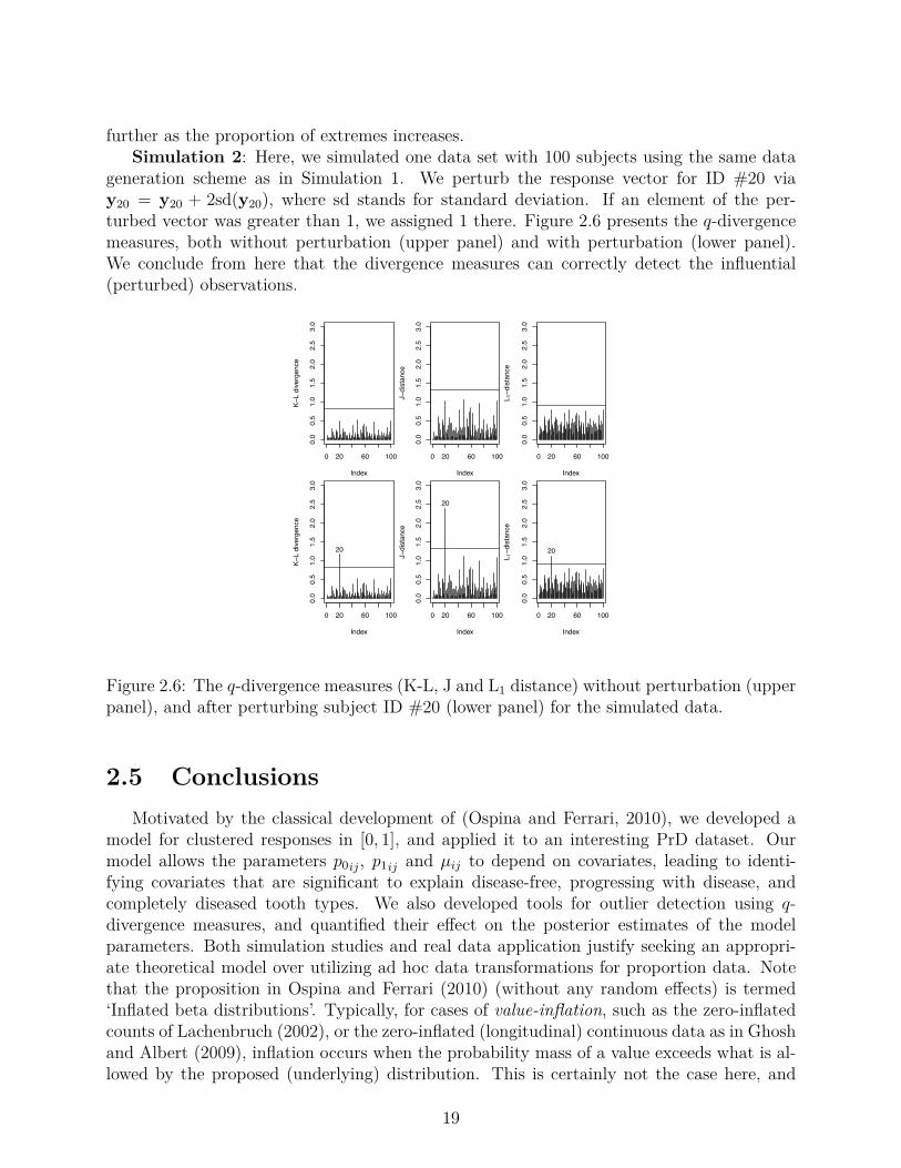
further as the proportion of extremes increases.Simulation 2: Here, we simulated one data set with 100 subjects using the same data

generation scheme as in Simulation 1. We perturb the response vector for ID #20 viay20 = y20 + 2sd(y20), where sd stands for standard deviation. If an element of the per-turbed vector was greater than 1, we assigned 1 there. Figure 2.6 presents the q-divergencemeasures, both without perturbation (upper panel) and with perturbation (lower panel).We conclude from here that the divergence measures can correctly detect the influential(perturbed) observations.

0 20 60 100

0.0

0.5

1.0

1.5

2.0

2.5

3.0

Index

K−L

dive

rgen

ce

0 20 60 100

0.0

0.5

1.0

1.5

2.0

2.5

3.0

Index

J−di

stan

ce

0 20 60 100

0.0

0.5

1.0

1.5

2.0

2.5

3.0

Index

L 1−d

ista

nce

0 20 60 100

0.0

0.5

1.0

1.5

2.0

2.5

3.0

Index

K−L

dive

rgen

ce

20

0 20 60 100

0.0

0.5

1.0

1.5

2.0

2.5

3.0

Index

J−di

stan

ce

20

0 20 60 100

0.0

0.5

1.0

1.5

2.0

2.5

3.0

Index

L 1−d

ista

nce

20

Figure 2.6: The q-divergence measures (K-L, J and L1 distance) without perturbation (upperpanel), and after perturbing subject ID #20 (lower panel) for the simulated data.

2.5 ConclusionsMotivated by the classical development of (Ospina and Ferrari, 2010), we developed a

model for clustered responses in [0, 1], and applied it to an interesting PrD dataset. Ourmodel allows the parameters p0

ij

, p1ij

and µij

to depend on covariates, leading to identi-fying covariates that are significant to explain disease-free, progressing with disease, andcompletely diseased tooth types. We also developed tools for outlier detection using q-divergence measures, and quantified their e�ect on the posterior estimates of the modelparameters. Both simulation studies and real data application justify seeking an appropri-ate theoretical model over utilizing ad hoc data transformations for proportion data. Notethat the proposition in Ospina and Ferrari (2010) (without any random e�ects) is termed‘Inflated beta distributions’. Typically, for cases of value-inflation, such as the zero-inflatedcounts of Lachenbruch (2002), or the zero-inflated (longitudinal) continuous data as in Ghoshand Albert (2009), inflation occurs when the probability mass of a value exceeds what is al-lowed by the proposed (underlying) distribution. This is certainly not the case here, and

19

following Hatfield et al. (2012), we prefer to call it an ‘augmented’ model over an ‘inflated’model. Our model can be fitted using standard available software packages, such as R andOpenBUGS, with easy access to practitioners in the field.

It is of interest to investigate the presence of thick/heavy tails in the underlying ZOAB-RE proposition, and to model the random e�ect term b

i

using robust alternatives (say, thet-density) over the normal density as in Figueroa-Zúniga et al. (2013). For our dataset, theresults were very similar using a t-density, and hence we did not consider it any further.

Our current analysis considers clustered cross-sectional periodontal proportion data. Of-ten, these study subjects can be randomized to dental treatments and subsequent longitudi-nal follow-ups, leading to a clustered-longitudinal framework, where one might be interestedin estimating the profiles (both overall, and subject-level) in the proportion of diseased sur-faces for the four tooth types with time. Our ZOAB-RE can certainly be extended to suchsituations with proper consideration to the GLMM REs specification. Other propositionsavailable in the literature on modeling clustered (or longitudinal) proportion responses in-clude simplex mixed-e�ects models (Qiu et al., 2008), robust transformation models (Songand Tan, 2000; Zhang et al., 2009), etc. How these models compare with ours, and ways toadapt these to proportion responses in [0, 1] are components of future research, and will beconsidered elsewhere.

20

Chapter 3

Augmented mixed models forclustered proportion data using thesimplex distribution

AbstractProportional continuous data can be found in areas such as biological sciences, health, engi-neering, etc. This type of data, doubly bounded, assumes values in the interval (0, 1) and foranalysis, distributions such as logistic-normal, beta, beta-rectangular and simplex, amongothers, have been used. However, because in practical situations it is possible to observe,proportions, rates or percentages that are zero and/or one, these distributions cannot beused. To deal with this, we propose a regression model based on the simplex distributionthat allows modelling the values zero and one simultaneously. For our analysis, we adopt aBayesian framework and develop a Markov chain Monte Carlo algorithm to carry out theposterior analyses for longitudinal proportional data. Bayesian case deletion influence diag-nostics based on the q-divergence measure and model selection criteria are also developed.We illustrated the proposed methodology through both simulation studies and real data todemonstrate the performance of our proposal.

Keywords Augmented distributions; Bayesian inference; MCMC; simplex distribution;q-divergence measures.

3.1 IntroductionDouble-bounded data can be found in di�erent areas such as biology, health sciences and

engineering, among many others. Some of the strategies pointed out in the statistical litera-ture to analyze this type of data are based on regression models combined with a particulardata transformation such as the logit transformation. However, the use of nonlinear trans-formations may hinder the interpretation of the regression parameters. This situation canbe overcome by considering probability distributions with double-bounded support, such asthe beta, simplex (Barndor�-Nielsen and Jørgensen, 1991), and beta rectangular distribu-tions (Hahn, 2008), which can be parameterized in terms of their mean. Other distributions,such as the logistic normal (Atchison and Shen, 1980) and the Kumaraswamy distribution

21

(Kumaraswamy, 1980) also have support in the unit interval. Nevertheless, the probabilitydensity function (pdf) of these distributions cannot be parameterized in terms of the means,limiting their use in regression analysis.

In this work, we focus on the simplex distribution to model proportions, rates or frac-tional data because its pdf presents a wide range of shapes including skewed, bimodal andmultimodal ones. Based on this distribution, Song and Tan (2000) proposed a regressionmodel relating the covariates with the mean via the logit link and assuming a fixed dispersionparameter. In that case, the the parameters are estimated through an extended version of thegeneralized estimating equations (GEE). Subsequently, Song et al. (2004) relaxed the con-dition over the dispersion parameter considering it to be heterogeneous as a function of thecovariates through the logarithm link function. On the other hand, Qiu et al. (2008) derivedthe penalized quasi-likelihood (PQL) and restricted maximum likelihood (REML) (Breslowand Clayton, 1993), using the high-order multivariate Laplace approximation, which givessatisfactory maximum likelihood (ML) estimation of the model parameters in the simplexmixed-e�ects model. More recently, López (2013) presented a Bayesian approach for estimat-ing the parameters in the simplex regression model where the response variable is confinedin the interval (0, 1).

In practical situations, proportions zero and/or one can be observed. Alternatives for theanalysis of this type of data (in the interval [0, 1]) consider some transformations such as thatproposed by Smithson and Verkuilen (2006). In this case, data values in the interval [0, 1] aretransformed to values in the interval (0, 1). Once the transformation is applied, distributionslike the beta or simplex, among others can be used. However, these transformations induceestimates with poor statistical properties even when small quantities of zeros and ones areobserved (Galvis et al., 2014). For that reason and motivated by our data application, whichincludes zeros and ones, we propose a zero and one augmented simplex model (ZOAS), whichallows us to deal with data in the interval [0, 1] without the need for transformations.

After fitting the model, it is important to conduct sensitivity analysis to detect possibleinfluential observations. An important approach to identify these influential cases is thecase-deletion method introduced by Cook (1977). In the Bayesian context, Xie et al. (2014)investigated the Bayesian estimation and case influence diagnostics for the zero-inflatedgeneralized Poisson regression model and Galvis et al. (2014) studied the Bayesian case-deletion diagnostics for the zero-and-one augmented beta random e�ects model. To thebest of our knowledge, the Bayesian approach for drawing influence diagnostics in ZOASrandom e�ects (ZOAS-RE) models has not been investigated in the literature. Therefore,an additional purpose of this work is to discuss and to develop some Bayesian influencediagnostic measures, based on the q-divergence, as proposed by Peng and Dey (1995), forthe ZOAS-RE model. These Bayesian measures can be easily implemented with standardBayesian software packages such as OpenBUGS (Thomas et al., 2006).

The paper is organized as follows. Section 3.2 presents some characteristics of the familyof dispersion models and introduces the simplex distribution as an element of this family.In addition, the ZOAS regression model and the ZOAS-RE model are presented. Section3.3 deals with the Bayesian inference, Bayesian model selection tools and case influencediagnostics for our proposed models. The application of the ZOAS-RE model is presentedin Section 3.4 and simulation studies are presented in Section 3.5. Finally, some concludingremarks and avenues for further research are presented in Section 3.6.

22

3.2 Statistical model3.2.1 Preliminaries

Dispersion models (DM) (Jørgensen, 1997) are a bi-parametric class of distributionswhose elements have a pdf given by

f(y|µ, ‡2) = a(y, ‡2) exp;

≠ 12‡2 d(y, µ)

<, (3.2.1)

where E[Y ] = µ, ‡2 > 0 is a dispersion parameter, a(y, ‡2) > 0 does not depend on µ andthe function d(·, ·) measures the discrepancy between the observed y and the expected µ.Through this function it is possible to identify each element belonging to the DM familyof distributions. This function is called unit deviance if it satisfies d(y, y) = 0 when y = µand d(y, µ) Ø 0 when y ”= µ. Moreover, the unit deviance is said to be regular if it is twicecontinuously di�erentiable with respect to (y, µ), satisfying ˆ

2

ˆµ

2 d(y, µ) = ˆ

2

ˆµ

2 d(y, y)---y=µ

> 0.

In this case (regular unit deviance), the variance function is defined as

V (µ) = 2I

ˆ2

ˆµ2 d(y, µ)---y=µ

J≠1

.

Some well known distributions such as the normal, gamma, inverse normal, binomialand Poisson, among others, are particular cases of the DM models and, additionally, belongto a subclass of the DM family called exponential dispersion models (EDM), as previouslyproposed by Jørgensen (1987). Note that our work is focused on the simplex distributionintroduced by Barndor�-Nielsen and Jørgensen (1991), which also belongs to the DM classof distributions. The simplex distribution is flexible and presents a wide variety of shapes,including some multimodal ones, which cannot be obtained by its counterpart, the betadistribution (see Figure 3.1). The pdf of a random variable Y following a simplex distribution,with mean µ and dispersion parameter ‡2, denoted by S(µ, ‡2), is given by

f(y|µ, ‡2) = {2fi‡2[y(1 ≠ y)]3}≠1/2 expI

≠ (y ≠ µ)2

2‡2y(1 ≠ y)µ2(1 ≠ µ)2

J

, (3.2.2)

where 0 < y < 1, 0 < µ < 1, ‡2 > 0.From the pdf (3.2.1), we have that a(y, ‡) = {2fi‡2[y(1 ≠ y)]3}≠1/2 and

d(y, µ) = ≠ (y ≠ µ)2

2‡2y(1 ≠ y)µ2(1 ≠ µ)2 . It can be shown that d(y, µ) is a regular unit deviance

and therefore the variance function for the simplex distribution is given by V (µ) = µ3(1≠µ)3.Figure 3.1 shows several shapes of the simplex distribution for some values of µ and

‡2. Note that, when µ is close to zero (one) and the value of ‡2 is large, the mass of thesimplex model is in the left (right) tail of the distribution. Moreover, when µ is close to 0.5and the value of ‡2 is large, the pdf of the simplex distribution is bimodal, unlike the betadistribution, which has a unique mode.

23

0.0 0.4 0.8

05

1015

y

f(y)

µ=0.1, !2=16

µ=0.1, !2=1

0.0 0.4 0.8

01

23

4

y

f(y)

µ=0.5, !2=16

µ=0.5, !2=1

0.0 0.4 0.8

01

23

45

6

y

f(y)

µ=0.7, !2=16

µ=0.7, !2=1

0.0 0.4 0.8

01

23

4

y

f(y)

µ=0.3, "=5µ=0.25, "=2

0.0 0.4 0.8

01

23

4

y

f(y)

µ=0.5, "=5µ=0.5, "=2

0.0 0.4 0.8

01

23

4

y

f(y)

µ=0.75, "=2µ=0.7, "=5

Figure 3.1: (Upper panel) pdf of the simplex distribution and (lower panel) pdf of the betadistribution with mean µ and precision parameter „.

3.2.2 Simplex regression modelIn order to define the simplex regression model, we consider the random variables y1, . . . , y

n

following the distribution given in (3.2.2). To relate the mean of the distribution with thecovariate vector x

i

, i = 1 . . . , n, we used a link function g1 with domain in the interval (0,1)and range on the real line. This function is given by g1(µi

) = x€i

—, where — is a vectorof regression parameters of dimension p where the first element of x

i

is equal to one to ac-commodate the intercept. The dispersion parameter ‡2 can be considered invariant for allsubjects as was adopted by Song and Tan (2000) and Qiu et al. (2008) or it can be regressedonto the covariates by using link functions such as the log, square root, etc, as was proposedby Song et al. (2004). The parameter estimation is conducted via ML in the classical contextor using a Markov chain Monte Carlo (MCMC) scheme in the case of the Bayesian approach.

3.2.3 Zero-and-one augmented simplex random e�ects modelTo deal with longitudinal data with observations in the [0, 1] interval, the ZOAS-RE

model is defined. Let Y1, . . . , Yn

be n random vectors, where Yi

= (Yi1, . . . , Y

ini)€ is aresponse vector of length n

i

corresponding to the i-th subject. In order to define the ZOAS-RE model, it is assumed that conditional on the random e�ects b

i

= (bi1, . . . , b

iq

)€, thecomponents Y

ij

of Yi

are independent and distributed according to the ZOAS model whose

24

pdf is given by

f(yij

|p0ij

, p1ij

, µij

, ‡2) =

Y_]

_[

p0ij

, if yij

= 0,p1

ij

, if yij

= 1,(1 ≠ p0

ij

≠ p1ij

)f(Yij

= yij

|µij

, ‡2), if yij

œ (0, 1),(3.2.3)

where f(yij

|µij

, ‡2) is as in (3.2.2), j = 1, . . . , ni

, p0ij

> 0, p1ij

> 0 and p0ij

+ p1ij

< 1. Wedenote by Y

ij

|bi

≥ ZOAS(µij

, ‡2, p0ij

, p1ij

) if the pdf of Yij

is given as in (3.2.3). Note that,in this case, the model parameters can be regressed onto some covariates using appropriatelink functions, as follows:

g1(µi

) = X€i

— + Z€i

bi

,

g2(p0i

) = W0€i

Â

andg3(p1

i

) = W1€i

fl,

where µi

= (µi1, . . . , µ

ini)€, bi

= (bi1, . . . , b

iq

)€ with bi· ≥ N(0, ‡2

b

), p0i

= (p0i1, . . . , p0

ini)€,

p1i

= (p1i1, . . . , p1

ini)€; X

i

, W0i

and W1i

are design matrices of dimension p ◊ ni

, r ◊ ni

and s ◊ ni

related to the fixed e�ects —, Â and fl respectively, and Zi

is the design matrixof dimension q ◊ n

i

related to the random e�ects vector bi

. Link functions as the logit,probit or complementary log-log can be considered for g1, g2 and g3. However, for the sakeof interpretation, here we choose the logit function. As was mentioned previously, ‡2 (as wellas the other parameters) can be regressed onto some covariates or considered invariant. Inthis work, we consider it invariant for all subjects. Finally, we define our ZOAS-RE modelas Y

ij

|bi

≥ ZOAS(µij

, ‡2, p0ij

, p1ij

), i = 1, . . . , n and j = 1, . . . , ni

.

3.3 Bayesian Inference3.3.1 Priors and posterior distributions

In order to complete the Bayesian specification, it is necessary to consider prior dis-tributions for all the unknown model parameters. In this case, we use Normal multi-variate distributions for the parameters —, Â and fl. That is, — ≥ Normal

p

(0, �≠1—

), ≥ Normal

r

(0, �≠1Â

), fl ≥ Normals

(0, �≠1fl

). For the dispersion parameter, we consid-ered a uniform distribution, which is ‡ ≥ Unif(0, a1) with a large value for a1. When thevector of probabilities (p0, p1, 1 ≠ p0 ≠ p1)€ is considered invariant, we use the Dirichlet priorwith hyperparameter –€ = (–1, –2, –3) and –

s

≥ Gamma(1, 0.001), s = 1, 2, 3. The priorfor the variance of RE is ‡

b

≥ Unif(0, b1), with a large positive value for b1. Although multi-variate specifications (multivariate zero mean vector with inverted-Wishart covariance) arecertainly possible, we stick to simple (and independent) choices.

Posterior conclusions are based on the joint posterior distribution of all the model pa-rameters (conditional on the data), and are obtained by combining the likelihoodL(�|b, X, Z, W0, W1, y) given by

nŸ

i=1

niŸ

j=1

1p0

ij

2Iyij =0 1

p1ij

2Iyij =1 Ë

(1 ≠ p0ij

≠ p1ij

)f(yij

; µij

, ‡2)È

Iyij œ(0,1),

25

and the joint prior densities using the Bayes’ rule. Thus, assuming a priori independence ofthe elements of the parameter vector, we can write

p(�, b, ‡b

|X, Z, W0, W1, y) Ã L(�|b, X, Z, W0, W1, y) ◊ fi(�, b, ‡b

),

where fi(�, b, ‡b

) = fi0(—)fi1(Â)fi2(fl)fi3(‡2)fi4(b|‡b

)fi5(‡b

) and fij

(.), j = 0, . . . , 5 denotesthe prior/hyperprior distributions for the model parameters as was described above.

The full conditional distributions necessary for the MCMC algorithm (a Metropolis-within-Gibbs algorithm) of the ZOAS-RE regression model are obtained as follows:

• fi(—|y, b, ‡b

, �(≠—)), is proportional to

expY]

[≠12(— ≠ —0)€�≠1

—

(— ≠ —0) ≠nÿ

i=1

niÿ

j=1

[yij

≠ (1 ≠ yij

)Aij

]2 (1 + Aij

)2

2‡2yij

(1 ≠ yij

)A2ij

I{yijœ(0,1)}

Z^

\ ,

where Aij

= exp(X€ij

— + Z€ij

bi

).

• fi(‡2|y, b, ‡b

, �(≠‡

2)) is a right truncated inverse gamma with truncation point a2. Thatis ‡2|y, b, ‡

b

, �(≠‡

2) ≥ IGamma+(a2, N ≠ 2,q

n

i=1q

nij=1 B

ij

), where N = qn

i=1 ni

and

Bij

= (yij

≠ µij

)2

2yij

(1 ≠ yij

)µ2ij

(1 ≠ µij

)2 , µij

= Aij

1 + Aij

and yij

œ (0, 1).

• fi(bi

|y, ‡b

, �) is proportional to

expY]

[≠12‡2

b

qÿ

k=1b2

ik

≠niÿ

j=1

[yij

≠ (1 ≠ yij

)Aij

]2 (1 + Aij

)2

2‡2yij

(1 ≠ yij

)A2ij

I{yijœ(0,1)}

Z^

\ I{bikœR}.

• When the probabilities p0 and p1 are regressed through some covariates,fi(Â|y, b, ‡

b

, �(≠Â)) is proportional to

exp;

≠12( ≠ Â0)€�≠1

Â

(Â ≠ Â0)<

nŸ

i=1

niŸ

j=1C

I{yij =0}ij

(1 ≠ Cij

≠ Dij

)I{yij œ(0,1)} ,

where Cij

= logit≠1(W0€ij

Â) and Dij

= logit≠1(W1€ij

fl); and fi(fl|y, b, ‡b

, �(≠fl)), isproportional to

exp;

≠12(fl ≠ fl0)€�≠1

fl

(fl ≠ fl0)<

nŸ

i=1

niŸ

j=1D

I{yij =1}ij

(1 ≠ Cij

≠ Dij

)I{yij œ(0,1)} .

• If p0 and p1 are considered invariant for all subjects, we have that fi(p|y, b, —, ‡b

)is a Dirichlet distribution with parameters (‹0, ‹1, ‹2), where ‹

l

= –l

qn

i=1q

nij=1 I

yij=l

,l = 0, 1 and ‹2 = –2

qn

i=1q

nij=1 I

yijœ(0,1).

26

The relevant MCMC steps were implemented using the BRugs package (Ligges et al., 2009),which connects the R with the OpenBUGS software. After discarding 50000 burn-in samples,we used 50000 more samples (with a spacing of 50) from two independent chains with widelydispersed starting values for posterior summaries. Convergence was monitored via MCMCchain histories, autocorrelation and crosscorrelation, density plots, and the Brooks-Gelman-Rubin potential scale reduction factor R̂, all of which are available in the R coda library(Cowles and Carlin, 1996). The associated BRugs code is available on request from thecorresponding author.

3.3.2 Bayesian model selection and influence diagnosticsWe use the conditional predictive ordinate (CPO) for our model selection derived from

the posterior predictive distribution (ppd), and summarize these CPOs via the log pseudo-marginal likelihood (LPML) statistic (Carlin and Louis, 2008). Larger values of LPMLindicate better fit. Owing to the instability of the harmonic-mean identity used for CPOcomputations (Raftery et al., 2007), we consider a more pragmatic route and compute theCPO (and LPML) statistics using 500 non-overlapping blocks of the Markov chain, each ofsize 2000, post-convergence (i.e., after discarding the initial burn-in samples), and reportthe expected LPML computed over the 500 blocks. In addition, we also apply the expectedAIC (EAIC), expected BIC (EBIC) (Carlin and Louis, 2008) and the DIC3 (Celeux et al.,2006) criteria. The DIC3 was used as an alternative to the usual DIC (Spiegelhalter et al.,2002) because of the ease of computation directly from the MCMC output, and also due tothe mixture modeling framework. All these criteria abide by the ‘lower is better’ law, i.e.,the model producing the lowest value gets selected.

In addition, as a direct by product of the MCMC output, some influence diagnosticmeasures are developed to study the impact of outliers on mainly the fixed e�ects parametersdue to data perturbation schemes based on case-deletion statistics (Cook and Weisberg,1982), and the q-divergence measures (Csisz et al., 1967; Weiss, 1996) between posteriordistributions. We consider three choices of these divergences, namely, the Kullback-Leibler(KL) divergence, the J-distance (symmetric version of the KL divergence), and the L1-distance. We use the calibration method of Peng and Dey (1995) to obtain the cut-o� valuesas 0.90, 0.83 and 1.32 for the L1, KL and J-distances, respectively.

3.4 Application to periodontal disease proportionsWe start this section with a brief description of the dataset. The Medical University

of South Carolina (MUSC) performed a study in order to know the status and progressionof clinical attachment level (CAL), a clinical marker of periodontal disease (PrD) amongGullah-speaking African-Americans with Type-2 diabetes. The main goal in that studyis to identify covariates related with absence, limited presence and total presence of thedisease. The dataset contain records on 28 teeth (considered full dentition, excluding the4 third-molars) from 290 subjects, where the attention is focused on quantifying the extentand severity of PrD with respect to tooth-types. The observed response is: ‘the proportionof diseased tooth-sites (with Cal value Ø 3mm), for each of the four tooth types, i.e.,

27

incisors, canines, pre-molars and molars, within a subject’, and therefore, a clustered dataframework is generated, where each subject records four observations corresponding to thefour tooth-types. Note that in this case, the response lies in the closed interval [0,1]; where0 and 1 represent completely disease free and highly diseased cases, respectively. Missingteeth were considered ‘missing due to PrD’ where all sites for that tooth contributed tothe diseased category. Subject-level covariates include Gender (0=male,1= female), Ageof subject at examination (in years), Glycosylated Hemoglobin (HbA1c) status indicator(0=controlled,< 7%; 1=uncontrolled,Ø 7%) and smoking status (0=non-smoker,1=smoker).The smokers category includes current and past smokers. We also considered a tooth-levelvariable, representing each of the four tooth-types, with ‘canine’ as the baseline.

Due to the presence of a substantial number of 0’s (114, 9.83%) and 1’s (94, 8.10%),the use of a simplex regression might be inappropriate in this context. Consequently, weconsider our proposed ZOAS-RE model in two di�erent setups:

Model 1 Yij

≥ ZOAS ≠ RE(µij

, ‡2, p0ij

, p1ij

),Model 2 Y

ij

≥ ZOAS ≠ RE(µij

, ‡2, p0, p1),where µ

ij

= logit≠1(X€ij

— + bi

), Xij

= (1, Genderi

, Agei

, HbA1ci

, Smokeri

,Incisor

ij

, Premolarij

, Molarij

)€, —0 is the intercept, —1, . . . , —7 are the regression parameters,and b

i

is the subject-level random e�ect term. For the parameters p0 and p1 we also uselogit link functions, that is, p0

ij

= logit≠1(W0€ij

Â) and p1ij

= logit≠1(W1€ij

Â) with W0ij

=W1

ij

= Xij

.We also consider in the analysis the zero and one augmented beta model with random

e�ects (ZOAB-RE) proposed by Galvis et al. (2014). This model uses the beta distributionparameterized as in Ferrari and Cribari-Neto (2004) to model data in (0, 1). In this model, asin the ZOAS-RE model, the parameters p0 and p1 can be considered constants or regressedonto covariates. Therefore, as in the case of the ZOAS-RE model, we consider two naturalcompeting models:

Model 3 Yij

≥ ZOAB ≠ RE(µij

, „, p0ij

, p1ij

),Model 4 Y

ij

≥ ZOAB ≠ RE(µij

, „, p0, p1).In these models, we consider the same systematic part and link function used in models 1and 2.

Although other link functions (such as probit, cloglog, etc) are available, here we restrictourselves to the symmetric logit link. Those models can be compared using the model choicecriteria described in Subsection 3.3.2. In the absence of historical data/experiments, our priorchoices follow the specifications described in Subsection 3.3.1. In the case of the parameter„ in the ZOAB-RE model, we consider a Gamma prior, that is, „ ≥ Gamma(0.1, 0.01).

Table 3.1 presents the DIC3, LPML, EAIC and EBIC values calculated for models 1-4.Notice that, Model 1 (ZOAS-RE model with covariates in p0 and p1) outperforms the othermodels for all criteria. Therefore, we select Model 1 as our best model. Figure 3.2 plots theposterior parameter means and the 95% credible intervals (CIs) for regression onto µ (leftpanel), p0 (middle panel) and p1 (right panel) from the models 1 and 3. The gray intervalsin this figure contain the zero value (the non-significant covariates), while the black intervalsdo not include the zero value (the significant ones at 5% level). In this figure, it can be notedthat the significance of the covariates is similar in both models. However, this significancechanges for the incisor covariate used to model µ, which is not significant under the Model1.

28

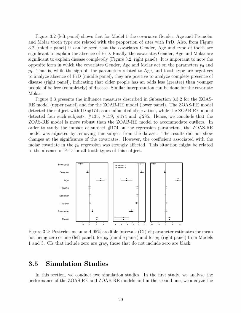
Figure 3.2 (left panel) shows that for Model 1 the covariates Gender, Age and Premolarand Molar tooth type are related with the proportion of sites with PrD. Also, from Figure3.2 (middle panel) it can be seen that the covariates Gender, Age and type of tooth aresignificant to explain the absence of PrD. Finally, the covariates Gender, Age and Molar aresignificant to explain disease completely (Figure 3.2, right panel). It is important to note theopposite form in which the covariates Gender, Age and Molar act on the parameters p0 andp1. That is, while the sign of the parameters related to Age, and tooth type are negativesto analyze absence of PrD (middle panel), they are positive to analyze complete presence ofdisease (right panel), indicating that older people has an odds less (greater) than youngerpeople of be free (completely) of disease. Similar interpretation can be done for the covariateMolar.

Figure 3.3 presents the influence measures described in Subsection 3.3.2 for the ZOAS-RE model (upper panel) and for the ZOAB-RE model (lower panel). The ZOAS-RE modeldetected the subject with ID #174 as an influential observation, while the ZOAB-RE modeldetected four such subjects, #135, #159, #174 and #285. Hence, we conclude that theZOAS-RE model is more robust than the ZOAB-RE model to accommodate outliers. Inorder to study the impact of subject #174 on the regression parameters, the ZOAS-REmodel was adjusted by removing this subject from the dataset. The results did not showchanges at the significance of the covariates. However, the coe�cient associated with themolar covariate in the p0 regression was strongly a�ected. This situation might be relatedto the absence of PrD for all tooth types of this subject.

Molar

Premolar

Incisor

Smoker

HbA1c

Age

Gender

Intercept

!2 0 2 4 !8 !6 !4 !2 0 2

Model 1Model 3

!10 !5 0 5 10

Figure 3.2: Posterior mean and 95% credible intervals (CI) of parameter estimates for meannot being zero or one (left panel), for p0 (middle panel) and for p1 (right panel) from Models1 and 3. CIs that include zero are gray, those that do not include zero are black.

3.5 Simulation StudiesIn this section, we conduct two simulation studies. In the first study, we analyze the

performance of the ZOAS-RE and ZOAB-RE models and in the second one, we analyze the

29

Model 1 Model 2 Model 3 Model 4DIC3 915.3 1165.3 993.0 1243.5

LPML -461.1 -584.1 -500.5 -623.7EAIC 917.8 1154.9 992.7 1231.0EBIC 1047.2 1210.5 1124.2 1286.6

Parameter mean SD mean SD mean SD mean SDIntercept ≠0.72s 0.20 ≠0.71s 0.21 ≠0.67s 0.18 ≠0.67s 0.18Gender ≠0.51s 0.18 ≠0.51s 0.17 ≠0.55s 0.16 ≠0.54s 0.17

Age 0.36s 0.08 0.37s 0.07 0.35s 0.07 0.34s 0.07HbA1c 0.05 0.15 0.04 0.15 0.08 0.14 0.07 0.15Smoker 0.11 0.16 0.10 0.17 0.11 0.16 0.12 0.15Incisor 0.14 0.09 0.15 0.09 0.20s 0.07 0.19s 0.07

Premolar 0.89s 0.09 0.89s 0.09 0.85s 0.07 0.85s 0.07Molar 2.17s 0.09 2.17s 0.09 2.15s 0.08 2.14s 0.08

‡2 7.25 0.40 7.26 0.41 - - - -„ - - - - 7.60 0.43 7.63 0.42p0 - - 0.098 0.009 - - 0.098 0.009p1 - - 0.081 0.008 - - 0.081 0.008‡2

b

1.33 0.14 1.30 0.13 1.22 0.11 1.22 0.13

Table 3.1: Posterior parameter (mean) estimates and standard deviations (SD) obtainedafter fitting Models 1-4 to the periodontal data. s denotes a significant parameter.

e�ect of transforming the observed zero and one values on the Bayesian estimates of theregression parameters.

In both studies, the data was generated from a logistic normal distribution (Atchison andShen, 1980), as follows. The location parameter µ

ij

was generated as: µij

= —0 + —1xij

+ bi

,with, b

i

≥ N(0, ‡2b

), i = 1, . . . , n, j = 1, . . . , 5, indicating a cluster of size 5. Then, wegenerated a random variable T

ij

following a normal distribution with mean µij

and variance1. Next, we obtained the random variable Y

ij

by applying the inverse logit of Tij

, that is,Y

ij

= logit≠1(Tij

). This strategy generates values for yij

in the interval (0, 1). The final stepis to allocate the 0’s, 1’s in the random sample y

ij

œ (0, 1). It is done by generating randomsamples from a multinomial distribution with probabilities vector (p0

ij

, p1ij

, 1 ≠ p0ij

≠ p1ij

)€

in simulation scheme 1 and (p0, p1, 1 ≠ p0 ≠ p1)€ in simulation scheme 2. The maingoal in both studies is to compare the mean squared error (MSE), relative bias, and coverageprobability for the regression parameter — = (—0, —1)€.

Simulation scheme 1

In this case, the parameters p0ij

and p1ij

are modeled through covariates as logit(p0ij

) =Â0 + Â1W0

ij

and logit(p1ij

) = fl0 + fl1W1ij

, respectively. The explanatory variables xij

andW1

ij

are generated as an independent draws from a Unif(0, 1) and W0ij

= W0i

is generatedas independent sample from a Bernoulli(0.8). The regression parameters and variance com-

30

0 50 150 250

0.0

0.5

1.0

1.5

2.0

2.5

3.0

Index

K!

L d

iverg

ence

174

ZOAS!RE Model

0 50 150 250

01

23

45

6

Index

J!

dis

tance

174

0 50 150 250

0.0

0.5

1.0

1.5

2.0

2.5

3.0

Index

L1!

dis

tance

174

0 50 150 250

0.0

0.5

1.0

1.5

2.0

2.5

3.0

Index

K!

L d

iverg

ence

174

ZOAB!RE Model

0 50 150 250

01

23

45

6

Index

J!

dis

tance

135159

174

285

0 50 150 250

0.0

0.5

1.0

1.5

2.0

2.5

3.0

Index

L1!

dis

tance

135

174

Figure 3.3: The q-divergence measures (K-L, J and L1 distances) for the application datausing the ZOAS-RE model (upper panel) and the ZOAB-RE model (lower panel).

ponents are fixed at —0 = ≠0.5, —1 = 0.5, Â0 = ≠1, Â1 = ≠1, fl0 = ≠1, fl1 = ≠1.5 and‡2

b

= 2, respectively.We simulated 200 data sets with di�erent sample sizes and fitted the ZOAS-RE and

the ZOAB-RE model with both, p0 and p1 modeled as explained above. In all cases sim-ilar priors were chosen as those used in Section 3.4. Using the parameter vector ◊ =(—0, —1, Â0, Â1, fl0, fl1, ‡2

b

), with ◊s

being an element of ◊, we calculate the MSE as MSE(◊̂s

) =1

200q200

i=1(◊̂is

≠ ◊s

)2, the relative bias as Relative Bias(◊̂s

) = 1200

q200i=1

1◊̂is◊s

≠ 12, and the 95%

coverage probability (CP) as CP(◊̂s

) = 1200

q200i=1 I(◊

s

œ [◊̂s,LCL

, ◊̂s,UCL

]), where I is the indi-cator function such that ◊

s

lies in the interval [◊̂s,LCL

, ◊̂s,UCL

], with ◊̂s,LCL

and ◊̂s,UCL

as theestimated lower and upper 95% CIs, respectively.

Figure 3.4 presents the results obtained for the parameters —0 and —1. It can be observedthat the ZOAS-RE model outperforms the ZOAB-RE model when the relative bias andCP are analyzed. However, both models exhibit similar MSE. The results related to theparameters Â0, Â1, fl0 and fl1 shown equal performance for both models, although this doesnot occur with the variance of the random e�ect, where the ZOAS-RE model outperformsthe ZOAB-RE model. In the ZOAS-RE model, the absolute relative bias is close to 20%for all sample sizes, while in the ZOAB-RE model the relative bias is close to 40%. Also,the MSE for the ZOAS-RE model decreases when the sample size increases. This is 0.31 forn = 50 and 0.21 for n = 200. In the case of the ZOAB-RE model, the MSE remains around0.60. Finally, the CP is greater for the ZOAS-RE model.

31

Further we fit the ZOAS-RE and ZOAB-RE models without covariates on p0 and p1. It ispossible to note that the performance of the relative bias, MSE and CP of the parameters —0,—1 and ‡2

b

of these models are very close to those obtained considering covariates on p0 andp1. Thus, we can conclude that considering p0 and p1 as constants, the Bayesian estimatesof the regression coe�cients —0 and —1 are not a�ected.

50 100 150 200

−1.2

−0.8

−0.4

0.0

0.2

n

Rel

ativ

e bi

as

β0

50 100 150 200

0.00

0.05

0.10

0.15

0.20

n

MS

E

ZOAS−RE ModelZOAB−RE Model

50 100 150 200

0.0

0.2

0.4

0.6

0.8

1.0

1.2

n

CP

50 100 150 200

−1.2

−0.8

−0.4

0.0

0.2

n

Rel

ativ

e bi

as

β1

50 100 150 200

0.00

0.05

0.10

0.15

0.20

n

MS

E

50 100 150 200

0.0

0.2

0.4

0.6

0.8

1.0

1.2

n

CP

Figure 3.4: Relative bias, MSE and CP of —0 and —1 after fitting the ZOAS-RE (black line)and ZOAB-RE (gray line) models for the simulated data.

Simulation scheme 2In this study, the parameters p0 and p1 are considered constants across all subjects by

assuming the probability values p0 = 1%, p1 = 1% in case a and p0 = 10%, p1 = 8% in caseb. Furthermore, the regression parameters and variance components are fixed at —0 = ≠0.5,—1 = 0.5 and ‡b

2 = 0.8. Using these values, we generated 200 datasets following the schemeabove and we fit our ZOAS-RE model and the simplex regression model (S-RE model) aftertransformation. The transformation used was that proposed by Smithson and Verkuilen(2006), where 0’s and 1’s are approximated by 1/2N and (2N ≠ 1)/2N , respectively, and Nis the total number of observations. The main goal of this study is to analyze the e�ect ofthis transformation on the estimates of the regression parameters —.

Figure 3.5 displays the results of Relative Bias, MSE and CP for the estimates of —0 and—1 in case a (upper panel) and case b (lower panel). As can be seen from this figure, eventhough the transformation of 0’s and 1’s is not prominent, there is a strong impact in thestatistical properties of the regression estimates. The results obtained in the variances ofRE are described next (figure not shown). In the ZOAS-RE model, the Relative Bias of ‡b

2is around of 20% for all sample sizes, while in the simplex counterpart, it starts at 0.34 for

32

n = 50 and greaches 1.34 for n = 200, indicating an increasing of the Relative Bias when thesample size increases. The MSE for this parameter is close to 5% in the ZOAS-RE model,but in the simplex model (transformed) it increases from 0.15 for n = 50 to 0.85 for n = 200.Also, when analyzing the CP, the ZOAS-RE model outperforms the (transformed) simplexmodel.

50 150

−1.2

−1.0

−0.8

−0.6

−0.4

−0.2

0.00.2

n

Relat

ive bi

as

β0

p0=p1=1%

50 150

0.00

0.05

0.10

0.15

0.20

0.25

0.30

n

MSE

50 150

0.00.2

0.40.6

0.81.0

1.2

n

CP

50 150

−1.2

−1.0

−0.8

−0.6

−0.4

−0.2

0.00.2

nRe

lative

bias

β1

ZOAS−RESimplex LS

50 150

0.00.1

0.20.3

0.40.5

0.60.7

n

MSE

50 150

0.00.2

0.40.6

0.81.0

1.2

n

CP50 150

−1.2

−1.0

−0.8

−0.6

−0.4

−0.2

0.00.2

n

Relat

ive bi

as

β0

p0=10%p1=8%

50 150

0.00

0.05

0.10

0.15

0.20

0.25

0.30

n

MSE

50 150

0.00.2

0.40.6

0.81.0

1.2

n

CP

50 150

−1.2

−1.0

−0.8

−0.6

−0.4

−0.2

0.00.2

n

Relat

ive bi

as

β1

50 150

0.00.1

0.20.3

0.40.5

0.60.7

n

MSE

50 1500.0

0.20.4

0.60.8

1.01.2

n

CP

Figure 3.5: Relative Bias, MSE and CP of —0 and —1 after fitting the ZOAS-RE (black line)and S-RE (gray line) models using (p0, p1)€ = (1%, 1%) (upper panel) and (10%, 8%) (lowerpanel).

3.6 ConclusionsThis article proposes a Bayesian random e�ect model based on the simplex distribution

for modeling data in the interval [0, 1]. The versatility of this class to model correlated datain the interval [0, 1] has not been explored elsewhere, and this is our major contribution. Sim-ulation studies reveal good consistency properties of the Bayesian estimates when comparedwith the beta regression counterpart, as well as, high performance of the model selectiontechniques to pick the appropriately fitted model. We also apply our method to a data setfrom periodontal disease conducted at the Medical University of South Carolina (MUSC) toillustrate how the procedures can be used to evaluate model assumptions, identify outliersand obtain unbiased parameter estimates. Although our modeling is primarily motivated

33

from periodontal disease data, it can be easily applied to other datasets, since the modelsconsidered in this article have been fitted using standard available software packages, like Rand OpenBUGS. This makes our approach easily accessible to practitioners of many fieldsof research. This paper complements the recently published work of Galvis et al. (2014),which also considers Bayesian estimation and inference of this kind of data by using the betadistribution (Ferrari and Cribari-Neto, 2004).

The models developed here do not consider skewness in the random e�ects and theirrobustness can be seriously a�ected by the presence of skewness and heavy tails in therandom e�ects. Recently, Lachos et al. (2009) adopted a Markov chain Monte Carlo approachto draw Bayesian inferences in linear mixed models with multivariate skew-normal (SNI)distributions in the random e�ects. Therefore, it would be a worthwhile task to investigatethe applicability of a Bayesian treatment in the context of ZOAS-RE models with SNIdistributions. Incorporating measurement error in covariates (Carrasco et al., 2014) withinour robust framework is also part of our future research.

34

Chapter 4

Augmented mixed models forclustered proportion data

AbstractOften in biomedical research, we deal with continuous (clustered) proportion responses rang-ing between zero and one quantifying the disease status of the cluster units. Interestingly,the study population might also consist of relatively disease-free as well as highly diseasedsubjects, contributing to proportion values in the interval [0, 1]. Regression on a variety ofparametric densities with support lying in (0, 1), such as beta regression, can assess impor-tant covariate e�ects. However, they are deemed inappropriate due the presence of zerosand/or ones. To evade this, we introduce a class of general proportion density (GPD), andfurther augment the probabilities of zero and one to this GPD, controlling for the clustering.Our approach is Bayesian, and presents a computationally convenient framework amenableto available freeware. Bayesian case-deletion influence diagnostics based on q-divergencemeasures are automatic from the MCMC output. The methodology is illustrated using bothsimulation studies and application to a real dataset from a clinical periodontology study.Keywords: Augment; Bayesian; Dispersion models; Kullback-Leibler divergence; Propor-tion data; Periodontal disease.

4.1 IntroductionContinuous proportion data (expressed as percentages, proportions, and rates), such as

the percent decrease in glomerular filtration rate at various follow-up times since baselineSong and Tan (2000); Kieschnick and McCullough (2003) are routinely analyzed in medicineand public health. Because the responses are confined in the open interval (0, 1), one mightbe tempted to use the logistic-normal model (Aitchison, 1986) with Gaussian assumptionsfor logit-transformed proportion responses. However, covariate e�ects interpretation arenot straightforward because the logit link is no longer preserved for the expected value ofthe response. Alternatively, to tackle this, the beta (Cepeda-Cuervo, 2001; Ferrari andCribari-Neto, 2004), beta rectangular (BRe) (Hahn, 2008) and simplex (Barndor�-Nielsenand Jørgensen, 1991) distributions (all with common support within the open unit interval),and their corresponding regressions were proposed under a generalized linear model (GLM)

35

framework.The flexible beta density (Johnson et al., 1994) can represent a variety of shapes, ac-

counting for uncorrectable non-normality and skewness (Smithson and Verkuilen, 2006) inthe context of bounded proportion data. The beta regression (BR) reparameterizes the as-sociated beta parameters, connecting the response to the data covariates through suitablelink functions (Ferrari and Cribari-Neto, 2004). Yet, the beta density does not accommodatetail-area events, or flexibility in variance specifications (Bayes et al., 2012). To accommodatethis, the BRe density Hahn (2008), and associated regression modelsBayes et al. (2012) wereconsidered under a Bayesian framework. Note, the BRe regression includes the (constantdispersion) BRFerrari and Cribari-Neto (2004), and the variable dispersion BR Smithsonand Verkuilen (2006) as special cases. The simplex regressionSong and Tan (2000) is basedon the simplex distribution from the dispersion family (Jørgensen, 1997), assumes constantdispersion, and uses extended generalized estimating equations for inference connecting themean to the covariates via the logit link. Subsequently, frameworks with heterogenous dis-persion (Song et al., 2004), and for mixed-e�ects models (Qiu et al., 2008) were explored.Yet, their potential were limited to proportion responses with support in (0, 1).

A clinical study on periodontal disease (PrD) conducted at the Medical University ofSouth Carolina (MUSC)(Fernandes et al., 2006) motivates our work. The clinical attachmentlevel (CAL), a clinical marker of PrD was measured at each of the 6 sites of a subject’s tooth,and we were interested to assess covariate-response relationships on ‘tooth-type specific (suchas incisors, canines, pre-molars and molars) proportion of diseased sites’ to determine thestatus of PrD. Figure 4.1 (left panel) plots the raw (unadjusted) density histogram of theproportion responses, packed over all subjects and tooth-types. The responses are in theclosed interval [0, 1] where 0 and 1 represent ‘completely disease free’, and ‘highly diseased’cases, respectively. For a simple parametric treatment to this data, one might be tempted touse one of the three distributions mentioned above after possible transformation Smithsonand Verkuilen (2006) of the response from [0, 1] to the interval (0, 1). These ad hoc re-scalings might work out for small proportions of 0’s and 1’s, but the sensitivity on parameterestimates can be considerable as the proportions increase. Transformations, in general,are not universal. In addition, presence of clustering (tooth-sites within mouth) brings in anextra level of heterogeneity, and these transformations which are usually applied component-wise may not guarantee a tractable (multivariate) joint distribution Jara et al. (2008). At thisstage, we desire an appropriate theoretical model capable of handling all these challenges,yet avoiding data transformations.

Note that the beta, BRe and simplex densities (and their regressions) present a notice-able analytic di�erence in their probability density function (pdf) specification. Motivatedby these di�erences and the flexibility they provide, we seek to combine them into a new(parametric) class of density called the general proportion density (GPD), where these threepopular models appear as particular cases. In this context, our paper generalizes the recentaugmented beta proposition Galvis et al. (2014). Next, we extend this GPD to a regressionsetup for independent responses in (0, 1). Finally, for a unified (regression) framework forclustered responses in [0, 1], we propose a generalized linear mixed model (GLMM) frame-work by augmenting the probabilities of occurrence of zeros, ones or both to the standardGPD regression model via an augmented GPD random e�ects (AugGPD-RE) model. Ourinferential framework is Bayesian, and can be easily handled using freeware like OpenBUGS.

36

Proportion CAL data

Densi

ty

0.0 0.2 0.4 0.6 0.8 1.0

0.00

0.02

0.04

0.06

0.08

0.10

0.12

0.0 0.2 0.4 0.6 0.8 1.0

0.00.1

0.20.3

0.40.5

0.60.7

0.80.9

1.0

Proportion CAL data

Cumu

lative

percen

t

Actual DataZOAS−RE ModelLS−simplex Model

Figure 4.1: Periodontal proportion data. The (raw) density histogram combining subjectsand tooth-types are presented in the left panel. The empirical cumulative distribution func-tion of the real data, and that obtained after fitting the ZOAS-RE and the LS-simplex modelsappear in the right panel.

Furthermore, case-deletion and local influence diagnostics (Peng and Dey, 1995) to assessoutlier e�ects are immediate from the Markov chain Monte Carlo (MCMC) output.

The rest of the article is organized as follows. Section 2 formulates the GPD and theaugmented GPD class of density as well as some useful statistical properties. Section 3 de-velops the Bayesian estimation framework for the AugGPD-RE regression model and relateddiagnostics. Application to the motivating PD data appear in Section 4. Section 5 presentssimulation studies to compare finite-sample performance of parameter estimates among theGPD class members, and also under model misspecification. Finally, some concluding state-ments appear in Section 6.

4.2 General proportion densityWe start with the definition of proportion density (PD) models, and then proceed to

establish the GPD density class.

Definition 1. A random variable (rv) › with support in the unit interval (0, 1) belongs tothe class of PD with parameters ⁄ and „ if it can be expressed as

g1(›; ⁄, „) = a1(⁄, „)a2(›, „) exp{≠„a3(›, ⁄)}, „ > 0, ⁄ œ (0, 1), (4.2.1)

where E[›] = ⁄, and as

(·, ·), s = 1, 2, 3 are real-valued functions with a1, a2 Ø 0, and a3 takingvalue on the real line. We use the notation › ≥ PD(⁄, „) to represent › a member of the PDclass defined in (4.2.1). Following Jørgensen (1997), if a3(›, ⁄) in (4.2.1) is continuous and

37

twice di�erentiable function with respect to › and ⁄ and is non-zero, the variance function

is V (⁄) = ≠A

ˆ2a3(›, ⁄)ˆ⁄ˆ›

B≠1 -----›=⁄

.

Next, consider the density of the rv X following the 2-component mixture X = ÷U +(1≠÷)›,where ÷ œ [0, 1] is a mixture parameter and U a Uniform(0, 1) rv distributed independentlyof › with pdf in (4.2.1). Then, X follows the general proportion density (GPD), i.e., X ≥GPD(÷, ⁄, „) with the pdf given by

g(X; ÷, ⁄, „) = ÷ + (1 ≠ ÷)g1(X; ⁄, „), (4.2.2)

where g1 is as defined in (4.2.1). Note that for ÷ = 1, the GPD reduces to the uniformdistribution, and for ÷ = 0 we retrieve the PD class of distributions. The mean and varianceof X are µ = E[X] = ÷/2 + (1 ≠ ÷)E[›], ‡2 = Var(X) = ÷

12 + (1 ≠ ÷)2Var(›), respectively.

4.2.1 Densities in the GPD classThe GPD class includes the beta, simplex, and the BRe densities with support in the

interval (0,1), and can be used to model proportion data. These are described in the propo-sitions below with their respective pdf’s presented in Appendix A.

Proposition 1. The beta density (Ferrari and Cribari-Neto, 2004) reparametrized in termsof µ (the mean) and of „ (the precision parameter) belongs to the GPD class of distributionswith its variance function given by V (µ) = µ(1 ≠ µ).

Proof. In (4.2.2), consider ÷ = 0, ⁄ = µ and g1(x; µ, „) = �(„)�(µ„)�((1 ≠ µ)„)xµ„≠1(1 ≠

x)(1≠µ)„≠1, such that a1(µ, „) = �(„)�(µ„)�((1 ≠ µ)„) , a2(x, „) =

1x(1 ≠ x)1≠„

2≠1and a3(x, µ) =

µ log 1≠x

x

. Then, the variance functionFerrari and Cribari-Neto (2004) (from Definition 1)is

V (µ) = ≠A

ˆ2a3(x, µ)ˆµˆx

B≠1 -----x=µ

= ≠A

≠1x(1 ≠ x)

B≠1 -----x=µ

= µ(1 ≠ µ)

.

Proposition 2. The simplex distribution (Barndor�-Nielsen and Jørgensen, 1991) with pa-rameters µ and „ belongs to the GPD class with the variance function given by V (µ) =µ3(1 ≠ µ)3.

Proof. In (4.2.2), consider ÷ = 0, ⁄ = µ and g1(x; µ, „) =Ô

„Ô

2fi (x(1 ≠ x))3/2

◊ expI

≠„(x ≠ µ)2

2x(1 ≠ x)µ2(1 ≠ µ)2

J

, such that a1(µ, „) = 1, a2(x, „) = „Ô

2fi (x(1 ≠ x))3/2

and a3(x, µ) = (x ≠ µ)2

2x(1 ≠ x)µ2(1 ≠ µ)2 . Then, the variance functionJørgensen (1997) isgiven by

V (µ) = ≠1

ˆ

2a3(x,µ)ˆµˆx

2≠1-----x=µ

= ≠1

≠1x

3(1≠x)3

2≠1-----x=µ

= µ3(1 ≠ µ)3.

38

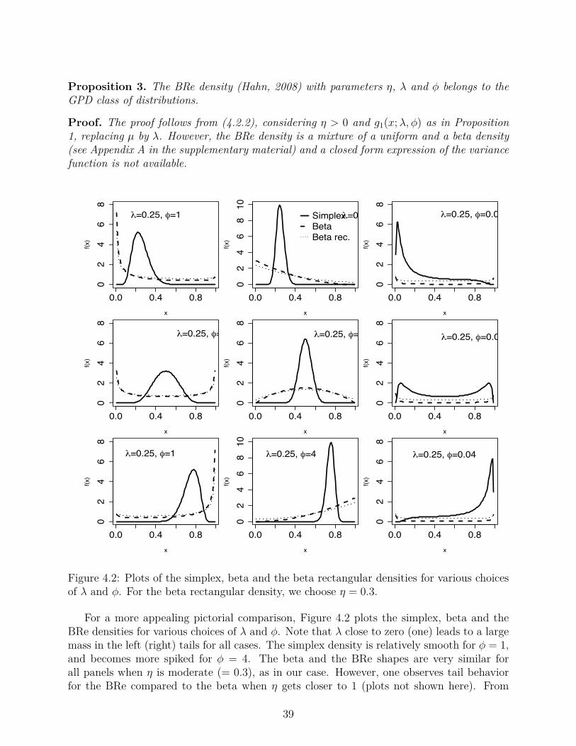
Proposition 3. The BRe density (Hahn, 2008) with parameters ÷, ⁄ and „ belongs to theGPD class of distributions.

Proof. The proof follows from (4.2.2), considering ÷ > 0 and g1(x; ⁄, „) as in Proposition1, replacing µ by ⁄. However, the BRe density is a mixture of a uniform and a beta density(see Appendix A in the supplementary material) and a closed form expression of the variancefunction is not available.

0.0 0.4 0.8

02

46

8

x

f(x)

λ=0.25, φ=1

0.0 0.4 0.8

02

46

810

x

f(x)

SimplexBetaBeta rec.

λ=0.25,

0.0 0.4 0.8

02

46

8

x

f(x)

λ=0.25, φ=0.04

0.0 0.4 0.8

02

46

8

x

f(x)

λ=0.25, φ=1

0.0 0.4 0.8

02

46

8

x

f(x)

λ=0.25, φ=4

0.0 0.4 0.8

02

46

8

x

f(x)

λ=0.25, φ=0.04

0.0 0.4 0.8

02

46

8

x

f(x)

λ=0.25, φ=1

0.0 0.4 0.8

02

46

810

x

f(x)

λ=0.25, φ=4

0.0 0.4 0.8

02

46

8

x

f(x)

λ=0.25, φ=0.04

Figure 4.2: Plots of the simplex, beta and the beta rectangular densities for various choicesof ⁄ and „. For the beta rectangular density, we choose ÷ = 0.3.

For a more appealing pictorial comparison, Figure 4.2 plots the simplex, beta and theBRe densities for various choices of ⁄ and „. Note that ⁄ close to zero (one) leads to a largemass in the left (right) tails for all cases. The simplex density is relatively smooth for „ = 1,and becomes more spiked for „ = 4. The beta and the BRe shapes are very similar forall panels when ÷ is moderate (= 0.3), as in our case. However, one observes tail behaviorfor the BRe compared to the beta when ÷ gets closer to 1 (plots not shown here). From

39

the plots, it is clear that the simplex density is more flexible than the two competitors. Itis capable of capturing various shapes of the underlying proportion data density in (0, 1),even in situations (say, small „) where the popular beta density may be far from the groundtruth. However, a major shortcoming of these densities is that they are not appropriate formodeling datasets containing proportion responses at the extremes (i.e., 0, or 1, or both).We seek to address this via an augmented GPD framework defined as follows:

Definition 2. The pdf of a rv Y with support in the interval [0, 1] belongs to the augmentedGPD class if it has the form

f(y; ÷, ⁄, „, p0, p1) = p0I{y=0} + p1I{y=1} + (1 ≠ p0 ≠ p1)g(y; ÷, ⁄, „)I{yœ(0,1)}, (4.2.3)

where I{A} is the indicator function of the set A; g(·) is as defined in Equation (4.2.2) andp0, p1 Ø 0, with p0 + p1 < 1.

From (4.2.3), the expectation and variance of Y are, respectively, E[Y ] = p1 + (1 ≠ p0 ≠p1)µ = ” and Var(Y ) = p1(1≠p1)+(1≠p0 ≠p1)[‡2 ≠2p1µ+(p0 +p1)µ2], where µ and ‡2 areas in Definition 1. Note, the augmented GPD class defined in (2) reduces to the GPD classwhen p0 and p1 are simultaneously equals to zero. When p0 > 0 and p1 = 0 we have the zeroaugmented GPD class, and for p0 = 0 and p1 > 0 we have the one augmented GPD class.Finally, when p0 > 0 and p1 > 0, we have the more general zero-one augmented GPD class.Motivated by the PrD data, we are particularly interested in the following three subfamiliesof the augmented GPD class, corresponding to the densities specified in Subsection 2.1

- Zero-one augmented beta (ZOAB) density, if ÷ = 0 and g1(·) the beta density

- Zero-one augmented simplex (ZOAS) density, if ÷ = 0 and g1(·) the simplex density

- Zero-one augmented beta rectangular (ZOABRe) density, if ÷ > 0 and g1(·) the betadensity

4.3 Model development and Bayesian inference4.3.1 GPD regression model

Let Y1, . . . , Yn

be n independent rv’s such that Yi

≥ GPD(÷i

, ⁄i

, „i

). Consider that µi

=÷

i

/2+(1≠÷i

)⁄ is directly modeled through covariates as g1(µi

) = x€i

— where g1 is a adequatelink function with counterdomain the real line, — is the vector of regression parameters withthe first element of x

i

being 1. However, µi

is a function of the mixture parameter ÷i

and⁄, which leads to a restricted parametric space of ÷

i

, defined as 0 < ÷i

< |2µi

≠ 1| that isdependent on µ

i

. Hence, for a more appropriate regression framework that connects Y tocovariates, we work with the reparameterization proposed in Bayes et al. (2012), and define–

i

œ [0, 1] such that –i

= ÷i

1 ≠ (1 ≠ ÷i

)|2⁄i

≠ 1| . Henceforth, the GPD class is parameterizedin terms of µ

i

, –i

and „i

.The parameters „

i

and –i

can be assumed constants, or regressed onto covariates throughconvenient link functions. For µ

i

and –i

, link functions such as, logit, probit or complemen-tary log-log can be used. Finally, for „

i

, the log, square-root, or identity link functions can

40

be considered. Parameter estimation can follow either the (classical) maximum likelihood(ML), or the Bayesian route through MCMC methods.

4.3.2 Augmented GPD random e�ects modelThe augmented GPD model described in (4.2.3) is only appropriate for independent

responses in (0, 1). To accommodate clustering (as in our case) or longitudinal subject-specific profiles, we proceed with the augmented GPD random e�ects (henceforth, AugGPD-RE) model. Let Y1, . . . , Y

n

be n independent continuous random vectors, where Yi

=(y

i1, . . . , yini)€ is the vector of length n

i

for the sample unit i, with the components yij

œ ’,where ’ is an element of the set {[0, 1), (0, 1], [0, 1]}. Thus, under the AugGPD-RE model,the parameters µ

ij

, p0ij

and p1ij

can be connected with covariates through suitable linkfunctions as

g1(E[Yi

|bi

]) = g1(µi

) = X€i

— + Z€i

bi

, (4.3.1)g2(p0

i

) = W0€i

Â, (4.3.2)g3(p1

i

) = W1€i

fl, (4.3.3)

where Xij

, W0ij

and W1ij

correspond to the j-th column from the design matrices Xi

,W0

i

and W1i

of dimension p ◊ ni

, r ◊ ni

and s ◊ ni

, related with the i-th unit sam-ple, corresponding to the vectors of fixed e�ects — = (—1, . . . , —

p

)€, Â = (Â1, . . . , Âr

)€,fl = (fl1, . . . , fl

s

)€, respectively, and Zi

is the design matrix of dimension q ◊ ni

correspond-ing to REs vector b

i

= (bi1, . . . , b

iq

)€. Choice of link functions for g1, g2 and g3 remainthe same as for µ

i

and –i

in Subsection 4.3.1. For purpose of interpretation, we focuson the logit link. In this work, we consider „ and – as constants despite those parame-ters can also be regressed onto covariates through suitable link functions. Also, to avoidover-parameterization, the probabilities p0

ij

and p1ij

are free of REs, however, both couldbe considered constants across subjects. Finally, we denote our AugGPD-RE model asY

ij

≥ AugGPD-RE(p0ij

, p1ij

, µij

, –, „) i = 1, . . . , n, j = 1, . . . , ni

.Let D = (X

i

, W0i

, W1i

, Zi

, y)€ be the full observed data and � = (—, Â, fl, „, –)€ bethe parameter vector in the AugGPD-RE model. The joint data likelihood, conditional onthe random-e�ects b

i

, L(�; D, b) is given by

L(�; b, D) =nŸ

i=1

niŸ

j=1p0

Iyij =0ij

p1Iyij =1ij

Ë(1 ≠ p0

ij

≠ p0ij

)g(yij

; –, µij

, „)È

Iyij œ(0,1), (4.3.4)

where p0ij

= logit≠1(W0€ij

Â), p1ij

= logit≠1(W1€ij

fl), I is an indicator function, and g isgiven by

g(yij

; –, µij

, „) = ÷ij

+ (1 ≠ ÷ij

)a1(⁄ij

, „)a2(yij

, „) exp {≠„a3(yij

, ⁄ij

)} , (4.3.5)

with ÷ij

= –(1 ≠ 2|µij

≠ 12 |), ⁄

ij

=µ

ij

≠ ÷ij

21 ≠ ÷

ij

and µij

= logit≠11X

µ

€ij

— + Zb

€ij

bi

2.

Although ML estimation of � is certainly feasible using standard softwares such as (e.g.,SAS, R, etc), we seek a Bayesian treatment here. The Bayesian approach accommodatesfull parameter uncertainty through appropriate choice of priors choices, proper sensitivity

41

investigations, and provides direct probability statement about a parameter through credibleintervals (C.I.) (Dunson, 2001). Next, we investigate the choice of priors on our modelparameters to conduct Bayesian inference.

4.3.3 Priors and posterior distributionsIn order to complete the Bayesian specification, we need to consider prior distributions

for all the unknown model parameters. In particular, we specify practical weakly informativeprior opinion on the fixed e�ects regression parameters —, Â, fl, „ (dispersion parameter),–, and the random e�ects b

i

. In general, for the regression components, we can assume— ≥ Normal

p

(0, �≠1—

), Â ≥ Normalr

(0, �≠1Â

), fl ≥ Normals

(0, �≠1fl

). A Uniform(0, 1) den-sityBayes et al. (2012) was adopted as prior for –. Prior on each element of b

i

are N(0, ‡2b

),where ‡

b

≥ Uniform(0, c1), the usual GelmanGelman (2006) specification. The prior on „for the specific models in Subsection 2.1 were chosen as follows:

(i) Beta and BRe models: „ ≥ Gamma(a, c), with small positive values of a and c (c π a).

(ii) Simplex model: „≠1/2 ≥ Uniform(0, a1), with large positive value for a1.

Assuming the elements of the parameter vector to be independent, the posterior conclu-sions are obtained combining the likelihood in (4.3.4), and the joint prior densities, givenby

p(�, b, ‡b

|D) Ã L(�; D) ◊ fi(�, b, ‡b

),where fi(�, b, ‡

b

) = fi0(—)fi1(Â)fi2(fl)fi3(–)fi4(„)fi5(b|‡b

)fi6(‡b

) and fij

(.), j = 0, . . . , 6 denotethe prior/hyperprior distributions on the model parameters as described above. The fullconditional distributions necessary for the MCMC algorithm (combination of Gibbs samplingand Metropolis-within-Gibbs) in the AugGPD-RE model are as follows:

• The full conditional density for Â|y, b, ‡b

, �(≠Â), fi1Â|y, b, ‡

b

, �(≠Â)

2is proportional

to

expÓ≠1

2€�≠1Â

ÂÔ nŸ

i=1

niŸ

j=1p0

Iyij =0ij

(1 ≠ p0ij

≠ p1ij

)Iyij œ(0,1) .

• The full conditional density for fl|y, b, ‡b

, �(≠fl), fi1fl|y, b, ‡

b

, �(≠fl)2

is proportionalto

expÓ≠1

2fl€�≠1fl

flÔ nŸ

i=1

niŸ

j=1p1

Iyij =1ij

(1 ≠ p0ij

≠ p1ij

)Iyij œ(0,1) .

• The full conditional density for —|y, b, ‡b

, �(≠—), fi1—|y, b, ‡

b

, �(≠—)

2is proportional

to

expÓ≠1

2—€�≠1—

—Ô nŸ

i=1

niŸ

j=1g(y

ij

; –, µij

, „)Iyij œ(0,1) , with g(yij

; –, µij

, „) given by (4.3.5).

42

• The full conditional density for „|y, b, ‡b

, �(≠„), fi(„|y, b, ‡b

, �(≠„)) is proportional to

fi(„)nŸ

i=1

niŸ

j=1g(y

ij

; –, µij

, „)Iyij œ(0,1) .

• The full conditional density for –|y, b, ‡b

, �(≠–), fi(–|y, b, ‡b

, �(≠–)) is proportional tonŸ

i=1

niŸ

j=1g(y

ij

; –, µij

, „)Iyij œ(0,1)I–œ[0,1].

• The full conditional density for bi

|y, ‡b

, �, fi(bi

|y, ‡b

, �) is proportional to

expI

≠qÿ

k=1

12‡2

b

b2ik

JniŸ

j=1g(y

ij

; –, µij

, „)Iyij œ(0,1) with bik

the k-th element of bi

= (bi1, . . . b

iq

)€.

• The full conditional density for ‡b

|y, b, �, fi(‡b

|y, b, �) is proportional to

expY]

[≠ 12‡

2b

nÿ

i=1

niÿ

j=1b2

ij

}

Z^

\ I‡bœ(0,c1).

For specific densities of the GPD class, the full conditionals for the beta, BRe and simplexmodels are presented in Appendix B. For computational simplicity, we avoid the multivariateprior specifications for —, Â and fl (multivariate zero mean vector with inverted-Wishartcovariance) and instead assign simple i.i.d Normal(0, Variance = 100) priors on the elementsof these vectors, which centers the ‘odds-ratio’ type inference at 1 with a su�ciently wide 95%interval. When p0 and p1 represent constant proportions for the whole data, we allocate theDirichlet prior with hyperparameter – = (–1, –2, –3)€ for the probability vector (p0, p1, 1 ≠p0 ≠ p1)€, with –

s

≥ Gamma(1, 0.01), s = 1, 2, 3. After discarding the first 50000 burn-insamples, we used 50000 more samples (with a spacing of 10) from 2 independent chainswith widely dispersed starting values for posterior summaries. Convergence was monitoredvia MCMC trace plots, autocorrelation plots and the Brooks-Gelman-Rubin R̂ statistics.Associated R code is available on request from the corresponding author.

4.3.4 Bayesian model selection and influence diagnosticsFor model selection, we use the conditional predictive ordinate (CPO) and the log pseudo-

marginal likelihood (LPML) statistic (Carlin and Louis, 2008), derived from the posteriorpredictive distribution (ppd). Larger values of LPML indicate better fit. Computing CPOvia the harmonic mean identity can lead to instability(Raftery et al., 2007). Hence, weconsider a more pragmatic route and compute the CPO (and LPML) statistics using 500non-overlapping blocks of the Markov chain, each of size 2000, post-convergence and reportthe expected LPML computed over the 500 blocks. In addition, we also apply the expectedAIC (EAIC), expected BIC (EBIC) (Carlin and Louis, 2008) and the DIC3 (Celeux et al.,2006) criteria. The DIC3 was used as an alternative to the usual DIC (Spiegelhalter et al.,2002) because of the ease of computation directly from the MCMC output, and also due tothe mixture modeling framework. All these criteria abide by the ‘lower is better’ law.

43

In addition, as a direct byproduct from the MCMC output, we develop some influencediagnostic measures to assess outlier e�ects on the fixed e�ects parameters based on case-deletion statistics (Cook and Weisberg, 1982), and the q-divergence measures (Csisz et al.,1967; Weiss, 1996) between posterior distributions. We consider three choices of these di-vergences, namely, the Kullback-Leibler (KL) divergence, the J-distance (symmetric versionof the KL divergence), and the L1-distance. We use the calibration methodPeng and Dey(1995) to obtain the cut-o� values as 0.90, 0.83 and 1.32 for the L1, KL and J-distances,respectively.

4.4 Data analysis and findingsThe motivating PrD dataset assessed the PrD status of Gullah-speaking African-Americans

with Type-2 diabetes via a detailed questionnaire focusing on demographics, social, medicaland dental history. The dataset contain measurements on 28 teeth (considered full dentition,excluding the 4 third-molars) from 290 subjects, recording proportion of diseased tooth-sites(with CAL value Ø 3mm) per tooth type as the response for each subject. Hence, thisclustered data framework has 4 observations (corresponding to the 4 tooth-types) for eachsubject. If a tooth is missing, it was considered ‘missing due to PrD’ where all sites forthat tooth contributed to the diseased category. Subject-level covariables in the datasetinclude gender (0=male,1= female), age of subject at examination (in years, ranging from26 to 87 years), glycosylated hemoglobin (HbA1c) status indicator (0=controlled,< 7%;1=uncontrolled,Ø 7%) and smoking status (0=non-smoker,1=smoker). We also considereda tooth-level variable representing each of the four tooth types, with ‘canine’ as the baseline.

From Figure 1 (left panel), the data are continuous on [0,1], with non-negligible pro-portions of of 0’s (114, 9.8%) and 1’s (94, 8.1%). Avoiding transformation, modeling viaone of the members of the GPD class might not be feasible. Hence, we proceed using theAugGPD-RE model, adjusted for subject-level clustering. From Equations (4.3.1), (4.3.2)and (4.3.3), we have

logit(µij

) = X€ij

— + bi

, (4.4.1)logit(p0

ij

) = W0€ij

Â,

logit(p1ij

) = W1€ij

fl,

where Xij

= (1, Genderij

, Ageij

, HbA1cij

, Smokerij

, Incisorij

, Premolarij

, Molarij

)€, Xij

=W0

ij

= W1ij

, — = (—0, . . . , —7)€, Â = (Â0, . . . , Â7)€ and fl = (fl0, . . . , fl7)€ are the vectors ofregression parameters, and b

i

is the subject-level random e�ect. The examination age wasstandardized (subtracting the mean and dividing by its standard deviation) to achieve betterconvergence. We have 6 competing models, varying with the densities in the GPD class andthe regression over p0 and p1, as follows:

Model 1 Yij

≥ ZOAS-RE(µij

, „, p0ij

, p1ij

).Model 1a Y

ij

≥ ZOAS-RE(µij

, „, p0, p1).Model 2 Y

ij

≥ ZOAB-RE(µij

, „, p0ij

, p1ij

).Model 2a Y

ij

≥ ZOAB-RE(µij

, „, p0, p1).Model 3 Y

ij

≥ ZOABRe-RE(–, µij

, „, p0ij

, p1ij

).Model 3a Y

ij

≥ ZOABRe-RE(–, µij

, „, p0, p1).

44

Note that the parameter – is specific to the ZOABRe model only. In addition, we alsofit the LS-simplex model (or Model 4) by transforming the response from y to yÕ via theLemon-squeezer (LS) transformation(Smithson and Verkuilen, 2006) given by yÕ = [y(N ≠1)+1/2]/N , where N is the number total of observations, with the regression on µ as (4.4.1).Although models 1, 1a, 2, 2a, 3 and 3a can be compared using standard model choice criteriadescribed in Subsection 4.3.4 because they fit the same dataset, this is not the case for theLS-simplex model which fits a transformed dataset. Thus, we assess its fit visually via theempirical cumulative distribution functions (ecdfs) of the fitted values. Table 4.1 presents

Criterion Model1 1a 2 2a 3 3a

DIC3 915.3 1165.3 993.0 1243.5 1001.3 1253.4LPML -461.1 -584.1 -500.5 -623.7 -503.8 -627.8EAIC 917.8 1154.9 992.7 1231.0 967.4 1210.4EBIC 1047.2 1210.5 1124.2 1286.6 1103.9 1281.2

Table 4.1: Model comparison using DIC3, LPML, EAIC and EBIC criteria.

the DIC3, LPML, EAIC and EBIC values for the 6 competing models. Notice that Model 1(ZOAS-RE model) provides the best fit uniformly across all criteria. Also, the fit for modelswith constant p0 and p1 are worser than the corresponding ones with regression on p0 and p1.The right panel of Figure 4.1 clear tells us that the ecdf from the fitted values using Model1 represent the true data much closely as compared to Model 4. Hence, we select Model 1as our best model and proceed with inference.

Molar

Premolar

Incisor

Smoker

HbA1c

Age

Gender

Intercept

−2 −1 0 1 2 3 4

Model 1Model 2Model 3Model 4

−8 −6 −4 −2 0 2 −4 −2 0 2

Figure 4.3: Posterior mean and 95% credible intervals (CI) of parameter estimates fromModels 1-4 for µ (left pannel), for p0 (middle pannel) and for p1 (right pannel). CIs thatinclude zero are gray, those that does not include zero are black.

45

Plots of the means of the posterior parameter estimates and their 95% CIs for the regres-sion onto µ (left panel), p0 (middle panel) and p1 (right panel) for Models 1-4 are presentedin Figure 4.3. We do not report the estimates from the models that consider p0 and p1as constants (i.e., Models 1a, 2a, and 3a). In this Figure, the gray intervals contain zero(non-significant covariates), while the black intervals do not include zero and are consideredsignificant at 5% level. From the left panel (regression onto µ

ij

), the covariates gender, ageand tooth-types significantly explain the proportion responses mostly for Models 1-4, withthe exception of Incisor for Model 1 where it is non-significant. Parameter interpretationcan be expressed in terms of its e�ect directly on µ

ij

, specifically µij

1≠µij, conditional on the

set of other covariates and REs Galvis et al. (2014). Here, µij

is the ‘expected proportionof diseased sites, and 1 ≠ µ

ij

is the complement, i.e., the ‘expected remaining proportion tobeing completely diseased’, both conditional on µ

ij

not being zero or one. These results areinterpreted in terms of the number of times the ratio is higher/lower with every unit increase(for a continuous covariate, such as age), or a change in category say from 0 to 1 (for a dis-crete covariate, say gender). For example, for age (a strong predictor of PrD), this ratio is1.43 (exp(0.36) = 1.43, 95% CI=[1.23, 1.66]) times higher for every unit increase in Age. ForGender, this ratio is 40% lower for males as compared to females, which might be influencedby the lower participation of males common in this population (Johnson-Spruill et al., 2009).Similarly, this ratio is 8.7 times higher for molars as compared to the canines (the baseline),which confirms that the posteriorly placed molars typically experience a higher PrD statusthan the anterior canines. From the plots in the middle and right panels of Figure 4.3, weidentify gender, age and tooth-types to be significant in explaining absence of PrD, whilegender, age and molar significantly explaining the completely diseased category. Once again,we have similar odds-ratio explanation as earlier. For example, the odds of a tooth type freeof PrD are 3 times greater for men than for women, while the odds of a completely dis-eased molar are about 13 times than of a (baseline) canine. Rest of the parameters can beinterpreted similarly.

The mean estimates (standard deviations) of „ from Models 1-4 are 0.14 (0.007), 7.6(0.43), 10.6 (1.56) and 0.002 (< 0.0001), and of ‡2

b

are 1.3 (0.13), 1.2 (0.13), 1.2 (0.13)and 2.6 (0.34), respectively. Due to parametrization involved, these estimates of „ are notcomparable across Models 1-3. However, the e�ect of the LS transformation is evident whilecomparing the estimates between Models 1 and 4. Additionally, the estimates of ‡2

b

revealthat the transformation in Model 4 leads to a higher (estimated) variance of the response Ythan the Models 1-3.

The adequacy of the logit link is assessed via plots of the linear predictor versus thepredicted probability (Hatfield et al., 2012) as depicted in the Figure in Appendix C. Con-sidering logit≠1(µ

ij

) from Model 1, we divided it into 10 intervals containing roughly anequal number of observations, and plot the distribution of the inverse-logit transformed lin-ear predictors (denoted by the black box-plots) that represents the fitted mean µ

ij

of thenon-zero-one responses. Next, we overlay the empirical distributions of the observed non-zero-one responses represented by the gray box-plots. There seem to be no evidence of modelmisspecification, i.e., the shapes of the fitted and observed trends are similar, as revealedfrom Figure C in the Appendix.

In addition, we conduct sensitivity analysis on the prior assumptions for the random

46

e�ects precision (1/‡2b

) and the fixed e�ects precision parameters on — by changing oneparameter at a time and refitting Model 1, as in (Galvis et al., 2014). In particular, weallowed ‡

b

≥ Uniform(0, k), where k œ {10, 50}, and also the typical Inverse-gamma choiceon the precision 1/‡2

b

≥ Gamma(k, k), where k œ {0.001, 0.1}. We also chose the normalprecision on the fixed e�ects to be 0.1, 0.25 (which reflects an odds-ratio in between e≠4

to e4) and 0.001. There were slight changes observed in parameter estimates and modelcomparison values, however, that did not change our conclusions regarding the best model,inference (and sign) of the fixed-e�ects, and the influential observations.

0 50 100 150 200 250 300

0.00.5

1.01.5

2.02.5

3.0

Index

K−L d

iverge

nce

KL di

verge

nce

ZOAS−RE Model

174

0 50 100 150 200 250 300

01

23

45

6

Index

J−dis

tance

J−dis

tance

174

0 50 100 150 200 250 300

0.00.5

1.01.5

2.02.5

3.0

Index

L1−d

istan

ce

174

0 50 100 150 200 250 300

0.00.5

1.01.5

2.02.5

3.0

Index

K−L d

iverge

nce

KL di

verge

nce

ZOAB−RE Model

174

0 50 100 150 200 250 300

01

23

45

6

Index

J−dis

tance

J−dis

tance

135159

174

285

0 50 100 150 200 250 300

0.00.5

1.01.5

2.02.5

3.0

Index

L1−d

istan

ce

135

174

0 50 100 150 200 250 300

0.00.5

1.01.5

2.02.5

3.0

Index

K−L d

iverge

nce

KL di

verge

nce

ZOABRe−RE Model

4 522

135159

174

285

0 50 100 150 200 250 300

01

23

45

6

Index

J−dis

tance

J−dis

tance

45

2231 86135159

174

285

0 50 100 150 200 250 300

0.00.5

1.01.5

2.02.5

3.0

Index

L1−d

istan

ce

4

5

2231 86135159

174

285

Figure 4.4: K-L, J and L1 divergences from the ZOAS-RE (upper panel), ZOAB-RE (middlepanel) and ZOABRe-RE (lower panel) models for the PrD dataset.

Finally, we detect outlying observations via the q-divergence measures for the augmentedmodels using the cut-o�s described in Subsection 4.3.4. These plots are presented in Fig-ure 4.4, where the upper, middle and lower panels represent the ZOAS-RE, ZOAB-RE andZOABRe-RE models, respectively. Interestingly, we find that the ZOABRe-RE model pro-duces several outlying observations exceeding the threshold, whereas the best-fitting model

47

(ZOAS-RE) produces only one such observation (subject id # 174). To quantify the impactof this observation, we refit the model by removing it. The covariate ‘Molar’ in the regressiononto p0

ij

is impacted by this observation, perhaps due to this subject is free of PrD for alltooth types. However, the parameter significance and sign of the coe�cients remained thesame. Henceforth, we stick to the estimates obtained from fitting Model 1 to the full data,without removing this particular subject.

4.5 Simulation studiesIn order to assess the finite sample performance of the class of AugGPD-RE mixed

regression models, we conduct two simulation studies. First (Scheme 1), we assess the impactof model misspecification on the parameters for the ZOAS-RE, ZOAB-RE and ZOABRe-REmodels when the data in (0,1) are generated from a logistic normal model (Atchison and Shen,1980). Next (Scheme 2), we analyze the impact of the LS transformation on the parameterestimates in presence of various proportions of zeros and ones. In both studies, we generatedata with various sample sizes, and compare the mean squared error (MSE), absolute relativebias (Abs.RelBias), and coverage probability (CP) of the regression parameters across thevarious models.

Initially, we generate yij

for both schemes and sample sizes n = 50, 100, 150, 200 asy

ij

= logit≠1(Tij

), i = 1, . . . , n (the number of subjects), j = 1, . . . , 5 (indicating cluster ofsize 5 for each subject), with T

ij

≥ Normal(µij

, 1) and the location parameter µij

modeledas µ

ij

= —0 + —1xij

+ bi

, with bi

≥ N(0, ‡2b

). The explanatory variables xij

are generated asindependent draws from a Uniform(0, 1), with the regression parameters fixed at —0 = ≠0.5,and —1 = 0.5, variance component ‡2 = 2, and constant proportions p0 = 0.1 and p1 = 0.1.Thus, y

ij

œ (0, 1) are draws from a logistic-normal model. Finally, via multinomial sampling,we allocate the 0’s, 1’s, and the y

ij

œ (0, 1) with probabilities p0, p1 and 1≠p0≠p1 respectively.No regression onto p0 and p1 are considered.

After simulating 200 such datasets, we fitted the ZOAS-RE, ZOAB-RE and ZOABRe-RE models with similar prior choices as in the data analysis. With our parameter vector◊ = (—0, —1, p0, p1, ‡2

b

), and ◊s

being an element of ◊, we calculate the MSE as MSE(◊̂s

) =1

200q200

i=1(◊̂is

≠ ◊s

)2, the absolute relative bias as Abs.RelBias (◊̂s

) = 1200

q200i=1| ◊̂is

◊s≠ 1|, and

the 95% coverage probability (CP) as CP(◊̂s

) = 1200

q200i=1 I(◊

s

œ [◊̂s,LCL

, ◊̂s,UCL

]), where I

is the indicator function such that ◊s

lies in the interval [◊̂s,LCL

, ◊̂s,UCL

], with ◊̂s,LCL

and◊̂

s,UCL

as the estimated lower and upper bounds of the 95% limits of the CIs, respectively.The results from this study for varying sample sizes are presented in Figure 4.5 and Table1 (Appendix D). Figure 4.5 presents a visual comparison of the models (bold line for theZOAS-RE model, dashed line for the ZOAB-RE model and dotted line for the ZOABRe-REmodel) for —0 (upper panel) and —1 (lower panel). For the sake of brevity, we do not produceplots for p0, p1 and ‡2

b

. We observe that the Abs.RelBias of both —0, —1 and ‡2b

are muchsmaller for the ZOAS-RE model as compared to the ZOAB-RE model and the ZOABRe-REmodels, while those for p0 and p1 are comparable. The MSEs of the parameters other than‡2

b

are comparable. For ‡2b

, the ZOAS-RE performs better (MSE is lower) than the othertwo. CP remains higher for the ZOAS-RE as compared to the other two models across all

48

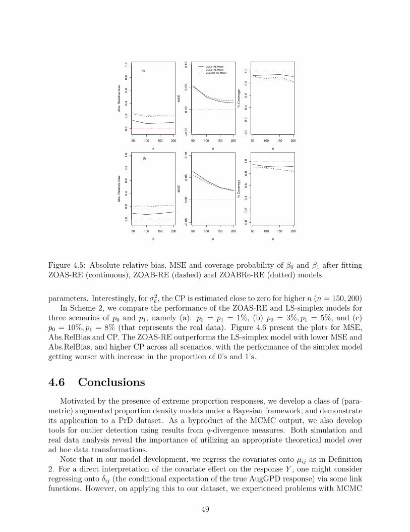
50 100 150 200

0.0

0.2

0.4

0.6

0.8

1.0

n

Abs

. Rel

ativ

e bi

as

β0

50 100 150 200

−0.0

50.

000.

050.

10

n

MS

E

ZOAS−RE ModelZOAB−RE ModelZOABRe−RE Model

50 100 150 200

0.0

0.2

0.4

0.6

0.8

1.0

n

% C

over

age

50 100 150 200

0.0

0.2

0.4

0.6

0.8

1.0

n

Abs

. Rel

ativ

e bi

as

β1

50 100 150 200

−0.0

50.

000.

050.

10

n

MS

E

50 100 150 200

0.0

0.2

0.4

0.6

0.8

1.0

n%

Cov

erag

e

Figure 4.5: Absolute relative bias, MSE and coverage probability of —0 and —1 after fittingZOAS-RE (continuous), ZOAB-RE (dashed) and ZOABRe-RE (dotted) models.

parameters. Interestingly, for ‡2b

, the CP is estimated close to zero for higher n (n = 150, 200)In Scheme 2, we compare the performance of the ZOAS-RE and LS-simplex models for

three scenarios of p0 and p1, namely (a): p0 = p1 = 1%, (b) p0 = 3%, p1 = 5%, and (c)p0 = 10%, p1 = 8% (that represents the real data). Figure 4.6 present the plots for MSE,Abs.RelBias and CP. The ZOAS-RE outperforms the LS-simplex model with lower MSE andAbs.RelBias, and higher CP across all scenarios, with the performance of the simplex modelgetting worser with increase in the proportion of 0’s and 1’s.

4.6 ConclusionsMotivated by the presence of extreme proportion responses, we develop a class of (para-

metric) augmented proportion density models under a Bayesian framework, and demonstrateits application to a PrD dataset. As a byproduct of the MCMC output, we also developtools for outlier detection using results from q-divergence measures. Both simulation andreal data analysis reveal the importance of utilizing an appropriate theoretical model overad hoc data transformations.

Note that in our model development, we regress the covariates onto µij

as in Definition2. For a direct interpretation of the covariate e�ect on the response Y , one might considerregressing onto ”

ij

(the conditional expectation of the true AugGPD response) via some linkfunctions. However, on applying this to our dataset, we experienced problems with MCMC

49

50 100 150 200

0.00.2

0.40.6

0.81.0

n

Abs.

Relat

ive bi

as

β0

p0=p1=1%

50 100 150 200

0.00.2

0.40.6

0.81.0

nMS

E

50 100 150 200

0.00.2

0.40.6

0.81.0

n

% C

overa

ge

ZOAS−RE ModelLS−simplex Model

50 100 150 200

0.00.2

0.40.6

0.81.0

n

Abs.

Relat

ive bi

as

β1

50 100 150 200

0.00.2

0.40.6

0.81.0

n

MSE

50 100 150 200

0.00.2

0.40.6

0.81.0

n

% C

overa

ge

50 100 150 200

0.0

0.2

0.4

0.6

0.8

1.0

n

Abs.

Rel

ative

bia

s

β0

p0=5% p1=3%

50 100 150 200

0.0

0.2

0.4

0.6

0.8

1.0

n

MSE

50 100 150 200

0.0

0.2

0.4

0.6

0.8

1.0

n

% C

over

age

50 100 150 200

0.0

0.2

0.4

0.6

0.8

1.0

n

Abs.

Rel

ative

bia

s

β1

50 100 150 200

0.0

0.2

0.4

0.6

0.8

1.0

n

MSE

50 100 150 200

0.0

0.2

0.4

0.6

0.8

1.0

n

% C

over

age

50 100 150 200

0.0

0.2

0.4

0.6

0.8

1.0

n

Abs.

Rela

tive

bias

β0

p0=10% p1=8%

50 100 150 200

0.0

0.2

0.4

0.6

0.8

1.0

n

MSE

50 100 150 200

0.0

0.2

0.4

0.6

0.8

1.0

n

% C

over

age

50 100 150 200

0.0

0.2

0.4

0.6

0.8

1.0

n

Abs.

Rela

tive

bias

β1

50 100 150 200

0.0

0.2

0.4

0.6

0.8

1.0

n

MSE

50 100 150 200

0.0

0.2

0.4

0.6

0.8

1.0

n

% C

over

age

Figure 4.6: Absolute relative bias, MSE and coverage probability of —0 and —1 after fittingZOAS-RE (continuous)and LS-simplex (dashed) models, for p0 = p1 = 1% (upper panel),p0 = 5%, p1 = 3% (middle panel) and p0 = 10%, p1 = 8% (lower panel).

convergence. Hence, we did not pursue it any further, although it may be appropriate forother datasets.

The current clustered setup can be extended to a longitudinal, or a clustered-longitudinalframework (often found in dental clinical trials). In addition, the current development ex-plores a simple parametric framework with ease in implementation. Certainly, the shapeof the proportion data can also be adequately captured via some (flexible) nonparametricspecification of the density. However, the Bayesian implementation may not be automatic,and would require developing customized MCMC algorithms. All these remain viable com-ponents of future research.

APPENDIXAPPENDIX A: Some densities in the GPD class

• The beta distributionThe density of a r.v Y following the beta distribution with mean µ and precision parameter

50

„ is given byf(y|µ, „) = �(„)

�(µ„)�((1 ≠ µ)„)yµ„≠1(1 ≠ y)(1≠µ)„≠1, (A1)

with 0 < E[Y ] = µ < 1, Var(Y ) = µ(1≠µ)1+„

and „ > 0.• The simplex distributionA r.v Y follows a simplex distribution with parameters µ and „ if its pdf is given by

f(y|µ, „) =Ô

„1fi [y(1 ≠ y)]3

21/2 expI

≠„(y ≠ µ)2

2y(1 ≠ y)µ2(1 ≠ µ)2

J

, (A2)

with 0 < E[Y ] = µ < 1 and „ > 0.• The beta rectangularA r.v Y is distribuited according to beta rectangular distribution with parameters ÷, ⁄ and„ if its pdf is given by

f(y|÷, ⁄, „) = ÷ + (1 ≠ ÷) �(„)�(⁄„)�((1 ≠ ⁄)„)y⁄„≠1(1 ≠ y)(1≠⁄)„≠1, (A3)

with 0 Æ ÷ Æ 1, 0 < ⁄ < 1, „ > 0, E[Y ] = ÷/2 + (1 ≠ ÷)⁄ and Var(Y ) = ⁄(1≠⁄)1+„

(1 ≠ ÷)(1 +÷(1 + „)) + ÷

12(4 ≠ 3÷).

APPENDIX B: Full conditional distributions from models ZOAS-RE, ZOAB-RE andZOABRe-RE in the augmented GPD class

The full conditional distributions of the parameters Â, fl and ‡b

necessary for the MCMCalgorithm in the three models above remain equal to presented for the augmented-GPD class.For the other parameters, the full conditional distributions are obtained for every model asfollows.ZOAS-RE model

• The full conditional density for —|y, b, ‡b

, �(≠—), fi1—|y, b, ‡

b

, �(≠—)

2is proportional

to

expY]

[≠12(— ≠ —0)€�≠1(— ≠ —0) ≠ „

nÿ

i=1

niÿ

j=1

[yij

≠ (1 ≠ yij

)Aij

]2 (1 + Aij

)2

2yij

(1 ≠ yij

)A2ij

Iyijœ(0,1)

Z^

\,

where Aij

= exp{X€ij

— + Z€ij

bi

}.

• The full conditional density for „|y, b, ‡b

, �(≠„), fi(„|y, b, ‡b

, �(≠„)) is a left truncatedgamma with left truncation point a≠2. That is „|y, b, ‡

b

, �(≠„) ≥ TGamma≠(a≠2, (n≠1)/2,

qn

i=1q

nij=1 a3(yij

, µij

)) where a3(yij

, µij

) = (yij≠µij)2

2yij(1≠yij)µ2ij(1≠µij)2 and µ

ij

= Aij

1+Aij.

• The full conditional density for bi

|y, ‡b

, �, fi(bi

|y, ‡b

, �) is proportional to

exp;

≠12‡

2b

qq

k=1 b2ik

≠ „q

nij=1

[yij≠(1≠yij)Aij ]2(1+Aij)2

2yij(1≠yij)A2ij

Iyijœ(0,1)

<I{bikœR}.

ZOAB-RE model

51

• The full conditional density for —|y, b, ‡b

, �(≠—), fi1—|y, b, ‡

b

, �(≠—)

2is proportional

to

expY]

[≠12(— ≠ —0)€�≠1(— ≠ —0) ≠

nÿ

i=1

niÿ

j=1

A

µij

„ log yij

1 ≠ yij

≠ Bij

B

Iyijœ(0,1)

Z^

\ ,

where Bij

= log �(µij

„) + log[�(1 ≠ µij

)„], µij

= Aij

1+Aij.

• The full conditional density for „|y, b, ‡2b

, �(≠„), fi(„|y, b, ‡2b

, �(≠„)) is proportional to

„a≠1 expY]

[≠„

Q

ac ≠nÿ

i=1

niÿ

j=1C

ij

Iyijœ(0,1)

R

b

Z^

\ ,

where Cij

= µij

log yij

1≠yij+ (1 ≠ µ

ij

) log(1 ≠ yij

) + log(„) ≠ Bij

and „ > 0.

• The full conditional density for bi

|y, ‡2b

, �, fi(bi

|y, ‡2b

, �) is proportional to

expY]

[≠12‡2

b

qÿ

k=1b2

ik

≠nÿ

i=1

niÿ

j=1

A

µij

„ log 1 ≠ yij

yij

≠ Bij

B

Iyijœ(0,1)

Z^

\ ,

with bik

œ R.

ZOABRe-RE model

• The full conditional density for —|y, b, ‡2b

, �(≠—), fi1—|y, b, ‡2

b

, �(≠—)

2is proportional

toexp

Ó≠1

2(— ≠ —0)€�≠1(— ≠ —0) + qn

i=1q

nij=1 I{yijœ(0,1)} log [÷

ij

+ (1 ≠ ÷ij

)Mij

]Ô

,

where Mij

= �(„)�(⁄ij„)�((1≠⁄ij)„)y

⁄ij„≠1ij

(1 ≠ yij

)(1≠⁄ij)„≠1, ÷ij

= –(1 ≠ 2|µij

≠ 12 |), ⁄

ij

=µij≠

÷ij2

1≠÷ijand µ

ij

= Aij

1+Aij.

• The full conditional density for „|y, b, ‡2b

, �(≠„), fi(„|y, b, ‡2b

, �(≠„)) is proportional to

„a≠1 expÓ≠„c + q

n

i=1q

n

i

j=1 I{yijœ(0,1)} log [÷ij

+ (1 ≠ ÷ij

)Mij

]Ô

,with „ > 0.

• The full conditional density for bi

|y, ‡2b

, �, fi(bi

|y, ‡2b

, �) is proportional to

exp;

≠12‡

2b

qnik=1 b2

ik

+ qn

i=1q

nij=1 I{yijœ(0,1)} log [÷

ij

+ (1 ≠ ÷ij

)Mij

]<

,

with bij

œ R.

• The full conditional density for –|y, ‡2b

, �, fi(–|y, ‡2b

, �) is proportional toexp

Óqn

i=1q

nij=1 I{yijœ(0,1)} log [÷

ij

+ (1 ≠ ÷ij

)Mij

]Ô

I{–œ[0,1]}.

52

APPENDIX C: Adequacy of the logit link

−1.7 −0.9 −0.2 0.5 1.4

0.0

0.2

0.4

0.6

0.8

1.0

Linear predictor (deciles)

E[Y|

Y≠

0,1]

−1.7 −0.9 −0.2 0.5 1.4

0.0

0.2

0.4

0.6

0.8

1.0

Figure 4.7: Observed and fitted relationship between the linear predictor and the (conditional)non-zero-one mean µ

ij

. Modeled logit relationships are represented by black box-plots, while theempirical proportions by gray box-plots.

53

APPENDIX D: Simulation Results from Scheme 1

ZOAS-RE model ZOAB-RE model ZOABRe-RE ModelParameter n = 50 n = 100 n = 150 n = 200 n = 50 n = 100 n = 150 n = 200 n = 50 n = 100 n = 150 n = 200

Abs.RelBias—0 0.13 0.08 0.09 0.10 0.23 0.19 0.20 0.20 0.25 0.21 0.21 0.20—1 0.09 0.07 0.09 0.11 0.19 0.19 0.20 0.21 0.21 0.20 0.21 0.22p0 0.02 0.02 0.00 0.0001 0.02 0.02 0.0003 0.00058 0.02 0.022 0.0009 0.0002p1 0.05 0.005 0.01 0.01 0.05 0.005 0.01 0.01 0.05 0.005 0.011 0.01‡2

b 0.19 0.20 0.22 0.226 0.37 0.38 0.40 0.40 0.38 0.38 0.40 0.40MSE

—0 0.05 0.03 0.02 0.01 0.05 0.03 0.02 0.02 0.05 0.03 0.02 0.19—1 0.06 0.04 0.03 0.02 0.06 0.04 0.03 0.02 0.06 0.04 0.03 0.02p0 0.0004 0.0002 0.0001 8e-05 0.0004 0.0002 0.0001 8e-05 0.0004 0.0002 0.0001 8e-0p1 0.0004 0.0001 0.0001 8e-05 0.0004 0.0001 0.0001 8e-05 0.0004 0.0001 0.0001 8e-0‡2

b 0.28 0.23 0.24 0.24 0.63 0.62 0.66 0.66 0.65 0.63 0.66 0.66CP

—0 0.92 0.93 0.94 0.91 0.91 0.88 0.90 0.83 0.90 0.89 0.87 0.81—1 0.95 0.91 0.91 0.91 0.90 0.90 0.86 0.83 0.90 0.88 0.85 0.85p0 0.94 0.92 0.93 0.96 0.94 0.93 0.93 0.97 0.94 0.91 0.92 0.95p1 0.94 0.95 0.94 0.96 0.92 0.95 0.94 0.96 0.93 0.95 0.94 0.96‡2

b 0.82 0.68 0.50 0.35 0.49 0.16 0.01 0.05 0.49 0.15 0.01 0.0

Table 4.2: Absolute Relative bias (Abs.RelBias), mean squared error (MSE), and coverageprobabilities (CP) of the the parameter estimates after fitting the ZOAS-RE, ZOAB-RE,and ZOABRe-RE models to simulated data for various sample sizes.

54

Chapter 5

Concluding remarks

5.1 ConclusionsMotivated by the presence of extreme proportion responses and the classical development

of (Ospina and Ferrari, 2010), it was developed a class of (parametric) augmented proportiondensity models under a Bayesian perspective, and demonstrated its application to a Peri-odontal dataset. In this model development, there were regressed covariates onto µ

ij

, p0ij

,p1

ij

, leading to identifying covariates that are significant to explain disease-free, progressingwith disease, and completely diseased tooth types. An alternative method (Smithson andVerkuilen, 2006) that transforms data was also studied and compared with the proposedmodels. Both simulation and real data analysis reveal the importance of utilizing an appro-priate theoretical model over ad hoc data transformations. There were also developed toolsfor outlier detection using q-divergence measures, and quantified their e�ect on the posteriorestimates of the model parameters.

Within the GPD class, the simplex density is more flexible than both its competitors.Hence, most likely the simplex regression (and its augmented counterpart) will outperformthe beta and the Bre regressions for relatively non-smooth proportion data, such as, datawith lots of spikes and structures, for support within (0, 1) (and [0, 1]). However, it is recom-mended a pragmatic modeling approach by fitting these 3 parametric densities successivelyto any dataset, and choosing the best one via popular model selection techniques.

5.2 Other publications• A Mixed-E�ect Model for Positive Responses Augmented by Zeros. Mariana Rodrigues-

Motta, Diana Milena Galvis Soto, Victor H. Lachos et al. Provisionally accepted paperin Statistics in Medicine. 2014.

• Bayesian semiparametric longitudinal data modeling using normal/independent densi-ties. Luis M. Castro, Victor H. Lachos, Diana M. Galvis and Dipankar Bandyopadhyay.Aceito para publicação em Chapman & Hall/CRC Press. Edited volume in “CurrentTrends in Bayesian Methodology with Applications”. 2014.

55

5.3 Future researchIt is of interest to investigate the presence of thick/heavy tails in the underlying ZOAB-

RE, ZOAS-RE and ZOABr-RE models, and to model the random e�ect term bi

using robustalternatives (say, the t-density) over the normal density as in Figueroa-Zúniga et al. (2013).For periodontal dataset, the results were very similar using a t-density, and hence we did notconsider it any further. The current analysis considers clustered cross-sectional periodontalproportion data. Often, these study subjects can be randomized to dental treatments andsubsequent longitudinal follow-ups, leading to a clustered-longitudinal framework, whereone might be interested in estimating the profiles (both overall, and subject-level) in theproportion of diseased surfaces for the four tooth types with time.

Certainly, the shape of the proportion data can also be adequately captured via some(flexible) nonparametric specification of the density. However, the Bayesian implementationmay not be automatic, and would require developing customized MCMC algorithms. Also,it is possible to include a e�ect that model the spatial relation that exist in the applicationdata as in Bandyopadhyay et al. (2011).

56

Bibliography

Aitchison, J. (1986). The Statistical Analysis of Compositional Data. London: Chapman &Hall.

Atchison, J. and S. M. Shen (1980). Logistic-normal distributions: Some properties anduses. Biometrika 67 (2), 261–272.

Bandyopadhyay, D., B. J. Reich, and E. H. Slate (2009). Bayesian modeling of multivariatespatial binary data with applications to dental caries. Statistics in Medicine 28, 3492–3508.

Bandyopadhyay, D., B. J. Reich, and E. H. Slate (2011). A spatial beta-binomial modelfor clustered count data on dental caries. Statistical Methods in Medical Research 20 (2),85–102.

Barndor�-Nielsen, O. E. and B. Jørgensen (1991). Some parametric models on the simplex.Journal of Multivariate Analysis 39 (1), 106–116.

Bayes, C. L., J. L. Bazán, and C. García (2012). A new robust regression model for propor-tions. Bayesian Analysis 7 (4), 841–866.

Branscum, A. J., W. O. Johnson, and M. C. Thurmond (2007). Bayesian Beta Regression:Applications to Household Expenditure Data and Genetic Distance Between Foot-and-Mouth Disease Viruses. Australian & New Zealand Journal of Statistics 49 (3), 287–301.

Breslow, N. E. and D. G. Clayton (1993). Approximate inference in generalized linear mixedmodels. Journal of the American Statistical Association 88 (421), 9–25.

Carlin, B. and T. Louis (2008). Bayesian Methods for Data Analysis (Texts in StatisticalScience). Chapman and Hall/CRC, New York.

Carrasco, J. M., S. L. Ferrari, and R. B. Arellano-Valle (2014). Errors-in-variables betaregression models. Journal of Applied Statistics 41 (7), 1–18.

Celeux, G., F. Forbes, C. P. Robert, and D. M. Titterington (2006). Deviance informationcriteria for missing data models. Bayesian Analysis 1 (4), 651–673.

Cepeda-Cuervo, E. (2001). Modeling variability in generalized linear models. Ph. D. thesis,Mathematics Institute, Universidade Federal do Rio de Janeiro.

Cook, R. D. (1977). Detection of influential observation in linear regression. Technomet-rics 19 (1), 15–18.

57

Cook, R. D. (1986). Assessment of local influence. Journal of the Royal Statistical Society,Series B 48, 133–169.

Cook, R. D. and S. Weisberg (1982). Residuals and influence in regression. Boca Raton,FL: Chapman & Hall/CRC.

Cowles, M. K. and B. P. Carlin (1996). Markov chain Monte Carlo convergence diagnostics:a comparative review. Journal of the American Statistical Association 91 (434), 883–904.

Csisz, I. et al. (1967). Information-type measures of di�erence of probability distributionsand indirect observations. Studia Sci. Math. Hungar. 2, 299–318.

Dey, D. K., M.-H. Chen, and H. Chang (1997). Bayesian approach for nonlinear randome�ects models. Biometrics, 1239–1252.

Dunson, D. (2001). Commentary: Practical advantages of Bayesian analysis of epidemiologicdata. American Journal of Epidemiology 153 (12), 1222.

Fernandes, J., C. Salinas, S. London, R. Wiegand, E. Hill, E. Slate, J. Grewal, P. Werner,J. Sanders, and M. Lopes-Virella (2006). Prevalence of periodontal disease in gullah africanamerican diabetics. Journal of Dental Research 85 (Special Issue A), 0997.

Ferrari, S. and F. Cribari-Neto (2004). Beta Regression for Modelling Rates and Proportions.Journal of Applied Statistics 31 (7), 799–815.

Figueroa-Zúniga, J. I., R. B. Arellano-Valle, and S. L. Ferrari (2013). Mixed beta regression:A Bayesian perspective. Computational Statistics & Data Analysis 61, 137–147.

Galvis, D. M., D. Bandyopadhyay, and V. H. Lachos (2014). Augmented mixed beta regres-sion models for periodontal proportion data. Statistics in Medicine 33 (21), 3759–3771.

Geisser, S. and W. F. Eddy (1979). A predictive approach to model selection. Journal ofthe American Statistical Association 74 (365), 153–160.

Gelman, A. (2006). Prior distributions for variance parameters in hierarchical models.Bayesian analysis 1 (3), 515–534.

Gelman, A., J. B. Carlin, H. S. Stern, and D. B. Rubin (2004). Bayesian Data Analysis.Chapman & Hall/CRC.

Ghosh, P. and P. S. Albert (2009). A Bayesian analysis for longitudinal semicontinuous datawith an application to an acupuncture clinical trial. Computational Statistics & DataAnalysis 53 (3), 699–706.

Hahn, E. D. (2008). Mixture densities for project management activity times: A robustapproach to PERT. European Journal of Operational Research 188 (2), 450–459.

Hatfield, L. A., M. E. Boye, M. D. Hackshaw, and B. P. Carlin (2012). Multilevel Bayesianmodels for survival times and longitudinal patient-reported outcomes with many zeros. J.Am. Stat. Assoc. 107, 875–885.

58

Jara, A., F. Quintana, and E. San Martín (2008). Linear mixed models with skew-ellipticaldistributions: A bayesian approach. Computational Statistics & Data Analysis 52 (11),5033–5045.

Johnson, N., S. Kotz, and N. Balakrishnan (1994). Continuous Univariate Distributions,Vol. 2. New York: John Wiley & Sons.

Johnson-Spruill, I., P. Hammond, B. Davis, Z. McGee, and D. Louden (2009). Healthof Gullah Families in South Carolina With Type 2 Diabetes Diabetes Self-managementAnalysis From Project SuGar. The Diabetes Educator 35 (1), 117–123.

Jørgensen, B. (1987). Exponential dispersion models. Journal of the Royal Statistical Society.Series B (Methodological), 127–162.

Jørgensen, B. (1997). The Theory of Dispersion Models, Volume 76. CRC Press.

Kieschnick, R. and B. D. McCullough (2003). Regression analysis of variates observed on(0, 1): percentages, proportions and fractions. Statistical Modelling 3 (3), 193–213.

Kumaraswamy, P. (1980). A generalized probability density function for double-boundedrandom processes. Journal of Hydrology 46 (1), 79–88.

Lachenbruch, P. A. (2002). Analysis of data with excess zeros. Statistical Methods in MedicalResearch 11 (4), 297–302.

Lachos, V. H., D. Bandyopadhyay, and D. K. Dey (2011). Linear and nonlinear mixed-e�ectsmodels for censored HIV viral loads using normal/independent distributions. Biomet-rics 67 (4), 1594–1604.

Lachos, V. H., L. M. Castro, and D. K. Dey (2013). Bayesian inference in nonlinear mixed–e�ects models using normal independent distributions. Computational Statistics & DataAnalysis 64, 237–252.

Lachos, V. H., D. K. Dey, and V. G. Cancho (2009). Robust linear mixed models withskew-normal independent distributions from a Bayesian perspective. Journal of StatisticalPlanning and Inference 139, 4098–4110.

Ligges, U., A. Thomas, D. Spiegelhalter, N. Best, D. Lunn, K. Rice, and S. Sturtz (2009).BRugs 0.5: OpenBUGS and its R/S-PLUS interface BRugs. http://www.stats.ox.ac.uk/pub/RWin/src/contrib.

López, F. O. (2013). A Bayesian approach to parameter estimation in simplex regressionmodel: a comparison with beta regression. Revista Colombiana de Estadística 36 (1), 1–21.

Ospina, R. and S. Ferrari (2010). Inflated beta distributions. Statistical Papers 51 (1),111–126.

Peng, F. and D. K. Dey (1995). Bayesian analysis of outlier problems using divergencemeasures. The Canadian Journal of Statistics 23, 199–213.

59

Qiu, Z., P. X.-K. Song, and M. Tan (2008). Simplex Mixed-E�ects Models for LongitudinalProportional Data. Scandinavian Journal of Statistics 35 (4), 577–596.

Raftery, A., M. Newton, J. Satagopan, and P. Krivitsky (2007). Estimating the integratedlikelihood via posterior simulation using the harmonic mean identity (with discussion). InJ. Berger, A. Dawid, D. Heckerman, A. Smith, and M. West (Eds.), Bayesian Statistics8, Volume 8, pp. 1–45. Oxford University Press.

Simas, A., W. Barreto-Souza, and A. Rocha (2010). Improved estimators for a general classof beta regression models. Computational Statistics and Data Analysis 54 (2), 348–366.

Smithson, M. and J. Verkuilen (2006). A better lemon squeezer? Maximum-likelihoodregression with beta-distributed dependent variables. Psychological Methods 11 (1), 54.

Song, P. X.-K., Z. Qi, and M. Tan (2004). Modelling heterogeneous dispersion in marginalmodels for longitudinal proportional data. Biometrical Journal 46 (5), 540–553.

Song, P. X.-K. and M. Tan (2000). Marginal models for longitudinal continuous proportionaldata. Biometrics 56 (2), 496–502.

Spiegelhalter, D. J., N. G. Best, B. P. Carlin, and A. van der Linde (2002). Bayesian measuresof model complexity and fit. Journal of the Royal Statistical Society-Series B 64 (4), 583–639.

Thomas, A., B. O’Hara, U. Ligges, and S. Sturtz (2006). Making BUGS open. R News 6 (1),12–17.

Verkuilen, J. and M. Smithson (2012). Mixed and mixture regression models for continuousbounded responses using the beta distribution. Journal of Educational and BehavioralStatistics 37 (1), 82–113.

Weiss, R. (1996). An approach to Bayesian sensitivity analysis. Journal of the Royal Statis-tical Society. Series B 58 (4), 739–750.

Xie, F.-C., J.-G. Lin, and B.-C. Wei (2014). Bayesian zero-inflated generalized poisson regres-sion model: estimation and case influence diagnostics. Journal of Applied Statistics 41 (6),1383–1392.

Zeileis, A., F. Cribari-Neto, and B. Grün (2010). Beta regression in R. Journal of StatisticalSoftware 34 (2), 1–24.

Zhang, P., Z. Qiu, Y. Fu, and P. X.-K. Song (2009). Robust transformation mixed-e�ects models for longitudinal continuous proportional data. Canadian Journal of Statis-tics 37 (2), 266–281.

60

Appendix A

BUGS code to implement theZOAB-Re model with covariates in p0and p1

model{Cte<-1000000

for(i in 1:n){b[i]~dnorm(0,tau)}

for(j in 1:N){zeros[j] <- 0zeros[j] ~ dpois(zeros.means[j])zeros.means[j] <- -lBetaInf[j]+CtefdBeta[j] <- exp(loggam(a1[j]+a2[j])-loggam(a1[j])-loggam(a2[j])

+(a1[j]-1)*log(Y[j])+(a2[j]-1)*log(1-Y[j]))a1[j] <- mu[j]*phia2[j] <- (1-mu[j])*philogit(mu1[j]) <- Beta[1] + Beta[2] * gender[j] + Beta[3] * age[j]

+ Beta[4] * hba1cd[j] + Beta[5] * smoker[j]+ Beta[6] * incisor [j] + Beta[7] * premolar[j]+ Beta[8] * molar[j] + b[cluster[j]]

mu[j] <- max(0.00001,min(0.9999,mu1[j]))logit(p0[j]) <- gamma[1] + gamma[2] * gender[j] + gamma[3] * age[j]

+ gamma[4] * hba1cd[j] + gamma[5] * smoker[j]+ gamma[6] * incisor [j] + gamma[7] * premolar[j]+ gamma[8] * molar[j]

logit(p1[j]) <- rho[1] + rho[2] * gender[j] + rho[3] * age[j]

61

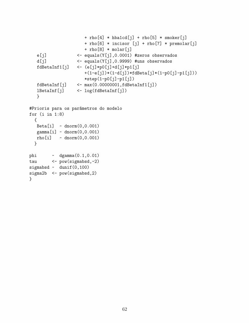
+ rho[4] * hba1cd[j] + rho[5] * smoker[j]+ rho[6] * incisor [j] + rho[7] * premolar[j]+ rho[8] * molar[j]

e[j] <- equals(Y[j],0.0001) #zeros observadosd[j] <- equals(Y[j],0.9999) #uns observadosfdBetaInf1[j] <- (e[j]*p0[j]+d[j]*p1[j]

+(1-e[j])*(1-d[j])*fdBeta[j]*(1-p0[j]-p1[j]))*step(1-p0[j]-p1[j])

fdBetaInf[j] <- max(0.00000001,fdBetaInf1[j])lBetaInf[j] <- log(fdBetaInf[j])}

#Prioris para os parâmetros do modelofor (i in 1:8)

{Beta[i] ~ dnorm(0,0.001)gamma[i] ~ dnorm(0,0.001)rho[i] ~ dnorm(0,0.001)

}

phi ~ dgamma(0.1,0.01)tau <- pow(sigmabsd,-2)sigmabsd ~ dunif(0,100)sigma2b <- pow(sigmabsd,2)}

62

Appendix B

Simulation results obtained when thesample is generated from ZOAB-REmodel

In this case, it was conducted a finite sample simulation study to investigate the conse-quences on parameter estimates after applying the LS transformation to the data in [0, 1]. Forthe data generation scheme, there were generated 100 samples of the ZOAB-RE model withthe location parameter µ

ij

is generated as: logit(µij

) = —0 + —1xij

+ bi

, with, bi

≥ N(0, ‡2),i = 1, . . . , n, j = 1, . . . , 5 indicating a cluster of size 5, and various choices of sample sizesn = 50, 100, 150, 200. The parameters „, p0 and p1 are considered constants, with values„ = 2, p0 = 0.1 and p1 = 0.1. The explanatory variables x

ij

= xi

, are generated as indepen-dent draws from a Bernoulli(0.8), and regression parameters and variance components arefixed at: —0 = 0.5, —1 = ≠0.5, and ‡2 = 4. This generates y

ij

’s in (0, 1). The final step is toallocate the 0’s, 1’s, and the y

ij

œ (0, 1), with probabilities p0, p1 and 1 ≠ p0 ≠ p1, which is aresult of multinomial draws.

63

ZOAB-RE model LS BetaParameter n = 50 n = 100 n = 150 n = 200 n = 50 n = 100 n = 150 n = 200

Relative bias—0 -0.115 -0.260 -0.264 -0.192 -0.613 -0.669 -0.666 -0.642—1 -0.076 -0.307 -0.235 -0.189 -0.603 -0.722 -0.678 -0.656„ 0.008 -0.008 -0.001 -0.010 -0.614 -0.648 -0.663 -0.675p0 0.052 0.004 0.001 0.011 - - - -p1 0.186 0.188 0.146 0.149 - - - -‡2 -0.193 -0.226 -0.235 -0.243 -0.893 -0.896 -0.898 -0.899

MSE—0 0,27 0,15 0,14 0,07 0,15 0,14 0,15 0,12—1 0,35 0,22 0,16 0,11 0,17 0,17 0,15 0,13„ 0,09 0,03 0,02 0,01 1,52 1,69 1,76 1,82p0 0,001 0,0001 0,0001 0,00001 - - - -p1 0,001 0,0001 0,0003 0,0003 - - - -‡2

b

0,96 0,97 0,98 1,05 12,81 12,87 12,91 12,95CP

—0 0,98 0,93 0,97 0,98 0,82 0,51 0,53 0,28—1 0,97 0,94 0,95 0,96 0,87 0,59 0,61 0,38„ 0,92 0,95 0,96 0,95 0,00 0,00 0,00 0,00p0 0,94 0,96 0,98 0,98 - - - -p1 0,81 0,76 0,72 0,67 - - - -‡2

b

0,90 0,60 0,49 0,31 0,00 0,00 0,00 0,00

Table B.1: Relative bias, MSE and CP for the parameters of ZOAB-RE and LS beta modelsusing di�erent sample size .

64

50 100 150 200

−1.2

−0.8

−0.4

0.0

0.2

n

Relat

ive b

ias

β0

50 100 150 200

−0.2

0.0

0.2

0.4

0.6

0.8

1.0

1.2

n

MSE

ZOAB−RE ModelLS Model

50 100 150 2000.

00.

20.

40.

60.

81.

01.

2

n

% C

over

age

50 100 150 200

−1.2

−0.8

−0.4

0.0

0.2

n

Relat

ive b

ias

β1

50 100 150 200

−0.2

0.0

0.2

0.4

0.6

0.8

1.0

1.2

n

MSE

50 100 150 200

0.0

0.2

0.4

0.6

0.8

1.0

1.2

n

% C

over

age

Figure B.1: Relative bias, MSE and CP for the parameters in ZOAB-RE and LS beta models.

65

Appendix C

Sensibility analysis for thehiperparameter of Dirichletdistribution

In order to analyse the sensibility of the hiperparameter of Dirichlet distribution, Itwas generated 50 sample of normal logistic distribution augmented by zeros and ones withparameters values —0 = ≠0.5, —1 = 0.5, p0 = 0.1, p1 = 0.08 and ‡2

b

= 2. Tables C.1 and C.2present the results about the relative bias and MSE when it is used the prior Gamma(1, 0.01)and Gamma(0.1, 0.01), respectively, in the models ZOAS-RE and ZOAB-RE.

ZOAS-RE modelRel. bias MSE

n=50 n=100 n=150 n=200 n=50 n=100 n=150 n=200—0 -0.10 -0.03 -0.08 -0.11 0.02 0.03 0.02 0.02—1 -0.09 -0.11 -0.10 -0.11 0.06 0.03 0.03 0.02p0 0.05 0.03 0.01 -0.0009 0.0003 0.0002 0.0001 0.00007p1 0.04 0.01 0.02 0.01 0.0002 0.0001 0.00009 0.00007‡2

b

-0.17 -0.22 -0.23 -0.23 0.32 0.26 0.26 0.25ZOAB-RE model

Rel. bias MSEn=50 n=100 n=150 n=200 n=50 n=100 n=150 n=200

—0 -0.23 -0.16 -0.20 -0.23 0.05 0.03 0.02 0.02—1 -0.20 -0.24 -0.22 -0.22 0.06 0.04 0.02 0.02p0 0.05 0.03 0.01 -0.0009 0.0003 0.0002 0.0001 0.00007p1 0.04 0.01 0.02 0.01 0.0002 0.0001 0.00009 0.00007‡2

b

-0.36 -0.40 -0.41 -0.41 0.60 0.68 0.70 0.69

Table C.1: Relative bias and MSE of the parameters in the ZOAS-RE and ZOAB-RE modelsobtained with the prior – ≥ Gamma(1, 0.01) in the hiperparameter of Dirichlet distribution

66

Modelo ZOAS-RERel. bias MSE

n=50 n=100 n=150 n=200 n=50 n=100 n=150 n=200—0 -0.02 -0.06 -0.08 -0.10 0.05 0.02 0.02 0.02—1 -0.09 -0.06 -0.06 -0.16 0.05 0.03 0.02 0.03p0 0.03 -0.02 -0.01 -0.01 0.0003 0.0001 0.0001 0.00007p1 0.03 0.04 -0.03 -0.01 0.0002 0.0002 0.0001 0.00007‡2

b

-0.18 -0.21 -0.22 -0.24 0.32 0.23 0.26 0.25Modelo ZOAB-RE

Rel. bias MSEn=50 n=100 n=150 n=200 n=50 n=100 n=150 n=200

—0 -0.15 -0.19 -0.21 -0.22 0.04 0.03 0.02 0.02—1 -0.20 -0.20 -0.20 -0.26 0.04 0.03 0.02 0.03p0 0.03 -0.03 -0.01 -0.01 0.0003 0.0002 0.0001 0.00007p1 0.03 0.04 -0.03 -0.01 0.0002 0.0002 0.0001 0.00007‡2

b

-0.37 -0.39 -0.41 -0.42 0.62 0.64 0.69 0.72

Table C.2: Relative bias and MSE of the parameters in the ZOAS-RE and ZOAB-RE modelsobtained with the prior – ≥ Gamma(0.1, 0.01) in the hiperparameter of Dirichlet distribu-tion.

67

Appendix D

Results about of simulation scheme 1in the Chapter 3.

ZOAS-RE model modelling p0 e p1 with covariatesRel. bias MSE CP

n=50 n=100 n=150 n=200 n=50 n=100 n=150 n=200 n=50 n=100 n=150 n=200—0 -0.10 -0.10 -0.12 -0.10 0.06 0.03 0.02 0.02 0.94 0.94 0.92 0.95—1 -0.10 -0.11 -0.13 -0.08 0.08 0.04 0.04 0.02 0.94 0.94 0.90 0.91‡

2b -0.18 -0.23 -0.22 -0.20 0.31 0.28 0.24 0.21 0.82 0.60 0.52 0.43

ZOAS-RE model with p0 and p1 constants across all observationsRel. bias MSE CP

n=50 n=100 n=150 n=200 n=50 n=100 n=150 n=200 n=50 n=100 n=150 n=200—0 -0.10 -0.11 -0.12 -0.11 0.06 0.03 0.02 0.02 0.96 0.94 0.92 0.94—1 -0.10 -0.11 -0.13 -0.08 0.08 0.04 0.04 0.02 0.95 0.95 0.90 0.90‡

2b -0.18 -0.23 -0.22 -0.20 0.31 0.28 0.24 0.21 0.82 0.60 0.52 0.43

Table D.1: Results of the scheme of simulation 1 presented in the chapter 3 where the datais analyzed of the ZOAS-RE model

ZOAB-RE model modelling p0 and p1 with covariatesRel. bias MSE CP

n=50 n=100 n=150 n=200 n=50 n=100 n=150 n=200 n=50 n=100 n=150 n=200—0 -0.23 -0.22 -0.23 -0.22 0.06 0.03 0.03 0.02 0.90 0.88 0.81 0.80—1 -0.25 -0.23 -0.25 -0.19 0.07 0.04 0.04 0.02 0.92 0.90 0.86 0.85‡

2b -0.36 -0.40 -0.40 -0.37 0.61 0.68 0.68 0.60 0.52 0.12 0.02 0.12

ZOAB-RE model with p0 and p1 constants across all observationsRel. bias EQM CP

n=50 n=100 n=150 n=200 n=50 n=100 n=150 n=200 n=50 n=100 n=150 n=200—0 -0.23 -0.22 -0.24 -0.22 0.06 0.03 0.03 0.02 0.91 0.89 0.81 0.80—1 -0.25 -0.23 -0.25 -0.19 0.07 0.04 0.04 0.02 0.93 0.89 0.86 0.84‡

2b -0.36 -0.40 -0.40 -0.37 0.61 0.68 0.68 0.60 0.50 0.12 0.02 0.12

Table D.2: Results of the scheme of simulation 1 presented in the chapter 3 where the dataanalized by the ZOAS-RE model

68