412TW-PA-15218

Bayes Tutorial using R and JAGS

James Brownlow

AIR FORCE TEST CENTER EDWARDS AFB, CA

12-14 May, 2015

4 1 2TW

Approved for public release ; distribution is unlimited. 412TW-PA-15218

AIR FORCE TEST CENTER EDWARDS AIR FORCE BASE, CALIFORNIA

AIR FORCE MATERIEL COMMAND UNITED STATES AIR FORCE

REPORT DOCUMENTATION PAGE Form Approved

OMB No. 0704-0188 Public reporting burden for this collection of information is estimated to average 1 hour per response, including the time for reviewing instructions, searching existing data sources, gathering and maintaining the data needed, and completing and reviewing this collection of information. Send comments regarding this burden estimate or any other aspect of this collection of information, including suggestions for reducing this burden to Department of Defense, Washington Headquarters Services, Directorate for Information Operations and Reports (0704-0188), 1215 Jefferson Davis Highway, Suite 1204, Arlington, VA 22202-4302. Respondents should be aware that notwithstanding any other provision of law, no person shall be subject to any penalty for failing to comply with a collection of information if it does not display a currently valid OMB control number. PLEASE DO NOT RETURN YOUR FORM TO THE ABOVE ADDRESS. 1. REPORT DATE 21/04/2015

2. REPORT TYPE ITEA tutorial

3. DATES COVERED (From - To)

4. TITLE AND SUBTITLE Bayes using R and JAGS

5a. CONTRACT NUMBER 5b. GRANT NUMBER 5c. PROGRAM ELEMENT NUMBER

6. AUTHOR(S) James Brownlow

5d. PROJECT NUMBER 5e. TASK NUMBER 5f. WORK UNIT NUMBER 7. PERFORMING ORGANIZATION NAME(S) AND ADDRESS(ES) AND ADDRESS(ES)

412 TSS/ENT 307 E. Popson Edwards AFB CA 92424

412TW-PA-15218

9. SPONSORING / MONITORING AGENCY NAME(S) AND ADDRESS(ES)

10. SPONSOR/MONITOR’S ACRONYM(S) N/A

11. SPONSOR/MONITOR’S REPORT NUMBER(S)

12. DISTRIBUTION / AVAILABILITY STATEMENT Approved for public release A: distribution is unlimited. 13. SUPPLEMENTARY NOTES CA: Air Force Test Center Edwards AFB CA CC: 012100

14. ABSTRACT Tutorial on how to obtain, load and use fundamental Bayesian analysis for flight test: examples include estimation of a binomial proportion, parameters of a normal distribution and reliability – homogeneous Poisson process trend estimation and prediction

15. SUBJECT TERMS

16. SECURITY CLASSIFICATION OF: Unclassified

17. LIMITATION OF ABSTRACT

18. NUMBER OF PAGES

19a. NAME OF RESPONSIBLE PERSON 412 TENG/EN (Tech Pubs)

a. REPORT Unclassified

b. ABSTRACT Unclassified

c. THIS PAGE Unclassified None 69

19b. TELEPHONE NUMBER (include area code)

661-277-8615 Standard Form 298 (Rev. 8-98)

Prescribed by ANSI Std. Z39.18

1

Bayes using R and JAGS

412th Test Wing

James Brownlow 812 TSS/ENT 661 277-4843

I n t e g r i t y - S e r v i c e - E x c e l l e n c e

Approved for public release; distribution is unlimited. 412TW-PA No.: 15218

War-Winning Capabilities … On Time, On Cost

12-14 May, 2015

2

Overview

• Introduction

• Background

• Uncertainty Analysis

• Systematic Error

• Random Error

• Conclusion

3

Goals

Load R, JAGS onto your laptop! (Disk set up for Windows)

Learn the fundamentals of Bayesian analyses Learn how to run Bayesian analyses from within R,

using JAGS, and interpret the results Learn how to evaluate “goodness of fit” for a Bayes

model Learn predictive posterior distributions, hierarchical

modeling

4

background

What is Bayesian data analysis? Why Bayes? Why R and Bugs Bayesian examples: binomial, normal distribution reliability applications

Model checking Bayes estimate and prediction of lambda in HPP reliability

analysis

5

What are BUGS and R?

Bugs – Bayesian analysis Using Gibbs Samplers BUGS is a language used to set up Bayesian inference JAGS (Just Another Gibbs Sampler) is the Bayes software

that runs within R R – GNU statistical analysis package

Open source language for statistical computing and graphics Well vetted, used in virtually every university on this planet

Bugs from within R Offers flexibility in data manipulation before the analysis and

display of inferences after Avoids tedious issues of working with Bugs directly

6

A brief prehistory of Bayesian data analysis

Reverend Thomas Bayes (1763) Links statistics to probability

Laplace (1800) Normal distribution Many applications, including census [sampling models]

Gauss (1800) Least squares Applications to astronomy [measurement error models]

Keynes, von Neumann, Savage (1920’s-1950’s) Link Bayesian statistics to decision theory

Applied statisticians (1950’s-1970’s) Hierarchical linear models Applications to medical trials, conjugate priors 1990s MCMC techniques, increased computing power

7

A brief history of Bayesian data analysis, BUGS, and R

“Empirical Bayes” (1950’s-1970’s) Estimate prior distributions from data

Hierarchical Bayes (from 1970) Include hyper parameters as part of the full model

Markov chain simulation (from 1940’s [physics] and 1980’s [statistics]) Computation with general probability models Iterative algorithms that give posterior simulations (not point estimates)

R code (open source) for statistical applications (1994) • lme() and lmer() functions by Doug Bates for fitting hierarchical linear and

generalized linear models

Bugs (from 1994) Bayesian inference Using Gibbs Sampling. Developed explicitly for

Bayesian statistics

8

What is Bayesian data analysis? Why Bayes?

Effective and flexible Combine information from different sources Examples of previous uses of Bayes from

flight test include: Radar systems analysis Regression testing (“same as old”) Reliability applications Multilevel regression, hierarchical modeling- test

unit parameters are not all the same, but are drawn from “parent” distribution

9

Structure of the tutorial

Computer use Example code included R, and JAGS “Follow along” computer demonstrations Feel free to Interrupt with questions Preliminaries include

How to set up a BUGS model in R Use R to facilitate posterior distribution

inference and diagnostics

10

Structure.. continued

Understanding how BUGS works and basic requirements for using JAGS with BUGS

Examples – Use Bayesian approach to Estimate the parameter of a binomial

distribution Estimate parameters of a log-normal

distribution Do reliability analysis- examine trend in an

assumed HPP

11

What are BUGS and R?

BUGS (Bayesian Inference Using Gibbs Sampling) Represent/Fit Bayesian statistical models Is a “language” designed to express Bayesian models

R Open source language for statistical computing and graphics

BUGS from within R Run MCMC based Bayesian analyses from within R Offers flexibility in data manipulation before the analysis and

display of inferences after Avoids tedious issues of working with Bugs directly

[Open R: binomial]

12

Bayes, Bugs, and R

Use R for data manipulations and various

analysis models Use BUGS within R to fit complex Bayesian

models User R to summarize results: Statistical inference from a posterior distribution check that fitted model makes sense (validity of

the BUGS) result check for validity of model implemented in BUGS

13

Fitting a Bayesian model in R and Bugs… We’ll cover

What’s required for a BUGS model Setting up data and initial values in R Running BUGS and checking results

(convergence, model adequacy) Displaying the posterior distribution, draw

inferences

EVERY R-script using JAGS looks like

1. Clear the workspace, get R2jags rm(list=ls()) require(R2jags) #interface: R and JAGS

2. Enter the “BUGS” model using R-function cat() …. As shown on next slide

14

Class Example: Estimate the probability of success of a rocket launch for companies

with limited launch/design experience

• Example is from Hamada et al., Bayesian Reliability, Springer, 2008

• Data: 11 companies with little launch/design experience. Objective is to develop a statistical model to predict launch success of a “new” company

• Model as a Bernoulli process- rocket launch was a success or it was not

15

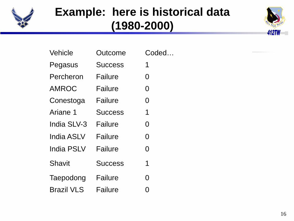
Example: here is historical data (1980-2000)

Vehicle Outcome Coded… Pegasus Success 1 Percheron Failure 0 AMROC Failure 0 Conestoga Failure 0 Ariane 1 Success 1 India SLV-3 Failure 0

India ASLV Failure 0

India PSLV Failure 0

Shavit Success 1

Taepodong Failure 0 Brazil VLS Failure 0

16

Begin with Maximum Likelihood Estimation of p

Probability of success is p, failure is (1-p)

f(y|n,p) = 𝑛𝑛𝑦𝑦 𝑝𝑝𝑦𝑦(1 − 𝑝𝑝)𝑛𝑛−𝑦𝑦

Log-likelihood: log[f(y|n,p)] α y * log(p) + (n-y) * log(1-p)

y = 3, n=11, take first derivative of log-likelihood, set =0,

0 = d( log(f(y|n,p))/d(p) = y/p - (n-y)/(1-p), solve for p

p = 3/11 = 0.272

17

Enter the BUGS model

• cat(‘ # model is a character string model { for(i in 1:n) { x[i] ~ dbern(theta) } theta ~ dbeta(1,1) #prior on theta }’ , # end of BUGS model file=“fileName.txt”) # end of cat()

18

19

R and Bugs for classical inference

Estimate the parameter of a binomial distribution using R / BUGS

Displaying the results in R or rmarkdown Use two priors for the analysis “vague” prior- uniform across (0,1) “informative” prior- p around 0.3

Required to run jags: data

fileNameData=list(x=c(rep(1,3), rep(0,8)), n=11)

• NOTE data must be a list()

20

Required to run jags: inits

fileNameInits = function() { list(theta = rbeta(1,1,1))} • NOTE inits must be a function, return a list

(allows for multiple MCMC chains) • Inits can be a NULL function- i.e. let JAGS

pick initial values of parameters

21

Required to run jags: parameters to save

fileNameParms = c(“theta”) • NOTE: parameters must be a text

“collection” (vector) of variable names

22

Summary, so far…

1. data must be a list 2. Inits must be a function 3. parameters must be a vector of text name(s)

of the variable(s) we want to examine, use for inference

23

Run jags

• Call to jags: (from within an R script) fileNameJags=jags( data=fileNameData, inits = fileNameInits, parameters.to.save = fileNameParms, model.file=“fileName.txt”, . .

24

Run jags continued

n.iter = 2000, n.thin = 1, n.burnin = 1000, n.chains = 4, DIC = TRUE) • Notice it’s all case sensitive!

25

Put together….

fileNameJags=jags( data = fileNameData, inits = fileNameInits, parameters.to.save = fileNameParms, model.file = “fileName.txt”, n.iter = 2000, n.thin = 1, n.burnin = 500, n.chains = 4, DIC = TRUE)

26

To get some diagnostics, and a plot:

fileNameJagsMC2 = autojags(fileNameJags)

attach.jags(fileNameJagsMC2)

plot(density(theta))

27

Now you try it! (exercise1.R)

Exercise: set up and run the binomial distribution- estimate theta, get a posterior density function of theta Use 3 successes in 11 trials Uniform prior distribution on p Parameter θ, plot posterior of θ Repeat using a beta distribution for prior p,

parameters (alpha=2.24, beta=2)

28

29

Overview of Bayesian data analysis

Decision analysis for reliability Where did the “prior distribution” come from? Simulation-based model checking

Result dependent on prior!

Different priors yielded different results! One can incorporate prior information into

analyses Prior distributions may be useful: Suppose we do a reliability test and have no

failures in 311 hours – what can we say about MTBF?

30

31

Decision analysis for reliability

Bayesian inference Prior(θ) + data + likelihood(data|θ) = posterior(θ) Where did the prior distribution come from?

32

Prior distribution

Example of Bayesian data analysis Binomial

Assume a beta prior for p Incorporate data to update estimate of p, MTBF On the disk- binomial.R

HPP model Number of failures proportional to interval length Poisson model On the disk– poisson.R

In both cases: model is flexible- add arbitrary time intervals, new data

33

More on Bayesian inference

Allows estimation of an arbitrary number of parameters

Summarizes uncertainties using probability Combines data sources Model is testable

OK, let’s, estimate p(successful launch) using Bayes..

MLE has excellent “large sample” properties, but, not so good for small to medium samples: large sample properties of MLE do not pertain

to complicated applications MLE is not appropriate for hierarchical models MLE does not work well when parameters are

close to boundary of the parameter space Deriving analytic expressions is difficult in

high-dimension situations All of these difficulties are, of course,

eliminated in Bayesian estimation

34

Fundamentals of Bayesian Inference

Frequentist estimation includes a confidence interval- i.e. an interval that will contain the true value of the parameter some specified proportion of the time in an infinite sequence of repetitions of the experiment

Bayesian estimation combines knowledge of the parameter available before sample data are analyzed with information gathered during an experiment Update the estimate of the parameter Summarize knowledge of the parameter using a

probability density function

35

Bayes fundamentals – the mechanism

∫=

=

θθθ

θθθ

dpyfym

ympyfyp

)()|()(

)()()|()|(

p(θ|y) is the posterior density of θ p(θ) is the prior density of θ m(y) is the marginal density of the data, and f(y|θ) is the sampling density of the data

36

And the parameter of interest, θ

θθθθ dyfE )|()( ∫=Once we get f(θ|y) we can estimate any density-related parameter!

37

The prior distribution

• In the launch vehicle example, θ is the parameter of interest, the probability of success of a launch

• Prior information: – Diffuse: θ can be anywhere in the interval (0,1) – Informative: more specific information about θ

may be available- past history indicates that θ is concentrated near 0.4

• We will look at the launch problem using first the “diffuse” (aka vague) prior and then the “informative” prior

38

Priors

• A priori we take all values in the interval (0,1) to be equally likely for θ: p(θ) = 1, 0 < θ < 1

• OR we use previous experience with launch vehicles to assert that the probably of a successful launch is around 0.55, and choose for the prior a beta distribution with parameters α=2.4, and β = 2 – Mean of the beta distribution is α/(α+β ) =

0.545, and – Median of the beta distribution is (α-1)/(α+β-1)

= 0.583

39

Beta prior for p

•

40

Likelihood function

• Likelihood = bernouli, so result is either 1, or 0 with probability p, repeated 11 times

• Can use a single likelihood, binomial- three successes in 11 trials

41

Now let’s use Bayes rule to estimate posterior distributions of the parameter, θ

• Bayes Rule: posterior α likelihood * prior • Implement this in the “BUGS” language • Call “jags” to develop the estimate of the

posterior distribution, f(θ |y)

42

EVERY R-script to use JAGS does the following

Clear the workspace, get R2jags rm(list=ls()) require(R2jags)

Enter the “BUGS” model using R-function

“cat()” …. As shown on next slide

43

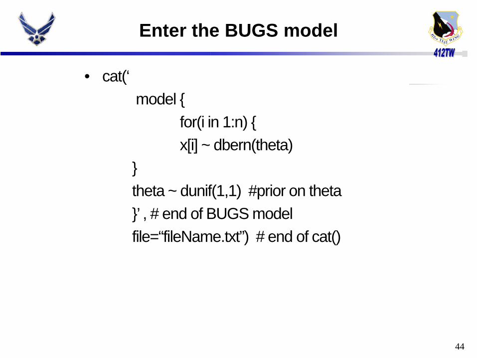
Enter the BUGS model

• cat(‘ model { for(i in 1:n) { x[i] ~ dbern(theta) } theta ~ dunif(1,1) #prior on theta }’ , # end of BUGS model file=“fileName.txt”) # end of cat()

44

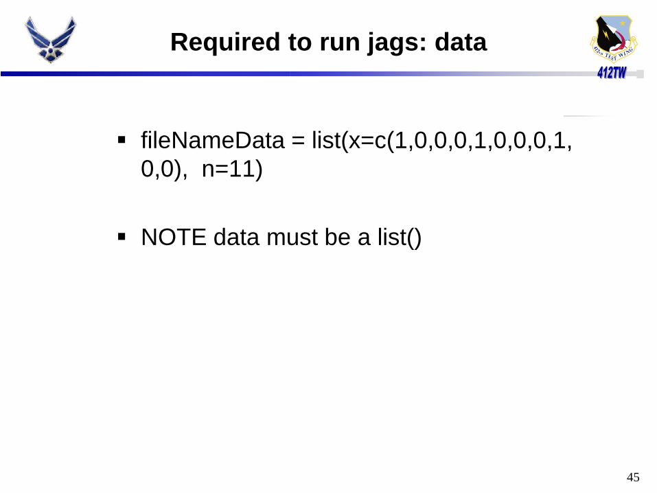
Required to run jags: data

fileNameData = list(x=c(1,0,0,0,1,0,0,0,1,

0,0), n=11)

NOTE data must be a list()

45

Required to run jags: inits

• fileNameInits = function() { list(theta = runif(1,0,1)) }

• NOTE “fileNameInits” must be a function,

return a list (allows for multiple MCMC chains)

46

Required to run jags: parameters to save

• fileNameParms = c(“theta”)

• NOTE: fileNameParms must be a text collection of one or more variable names

47

Quick Check: need to input data, inits, and parameters to save

1. data must be a list 2. Inits must be a function 3. parameters must be a collection of text,

naming variables we want to examine

48

Run jags

• Call to jags: • fileNameJags=jags( data=fileNameData, inits = fileNameInits, parameters.to.save = fileNameParms, model.file=“fileName.txt”, . .

49

Run jags continued

n.iter = 2000, n.thin = 1, n.burnin = 1000, n.chains = 4, DIC = TRUE)

• Notice it’s all case sensitive!

50

Put together….

• fileNameJags=jags( data = fileNameData, inits = fileNameInits, parameters.to.save = fileNameParms, model.file = “fileName.txt”, n.iter = 2000, n.thin = 1, n.burnin = 1000, n.chains = 4, DIC = TRUE)

51

Get some diagnostics, and a plot

fileNameJagsMC2 = autojags(fileNameJags)

attach.jags(fileNameJagsMC2)

plot(density(theta))

52

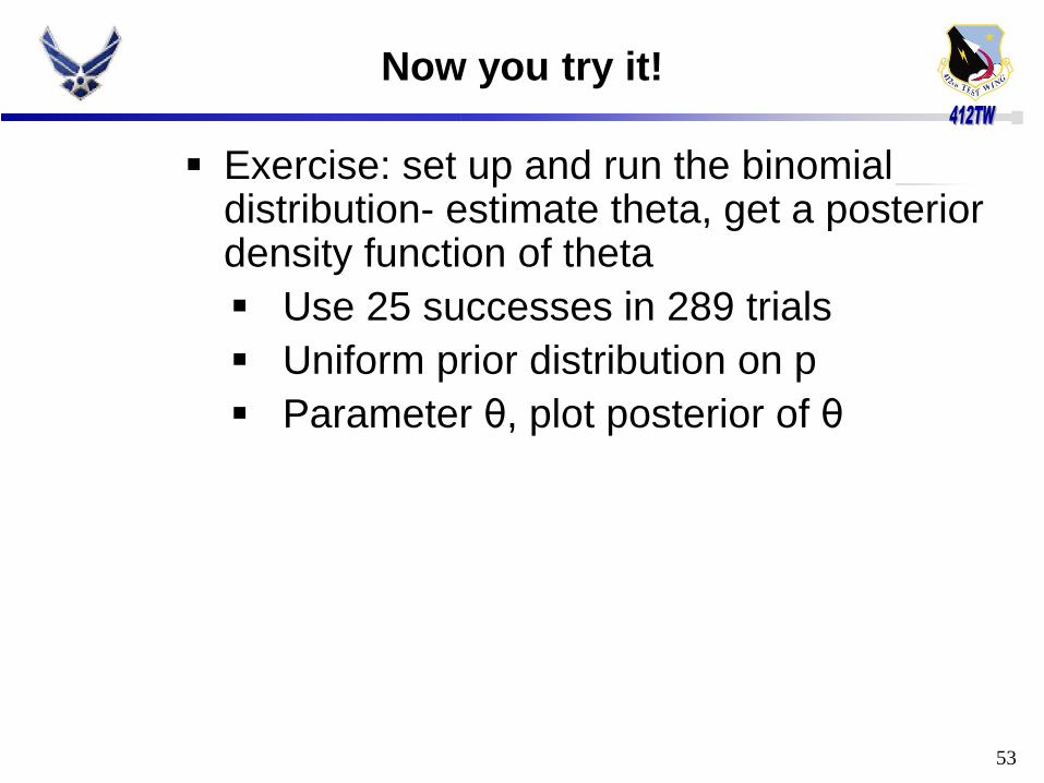
Now you try it!

Exercise: set up and run the binomial distribution- estimate theta, get a posterior density function of theta Use 25 successes in 289 trials Uniform prior distribution on p Parameter θ, plot posterior of θ

53

54

Decision analysis for reliability

Bayesian inference

Prior(θ) + data + likelihood(data|θ) = posterior(θ) Where did the prior distribution come from?

55

Prior distribution

Example of Bayesian data analysis HPP model

Number of failures proportional to interval length Poisson model On the disk– poisson.R

Data model Flexible: arbitrary time intervals, Add data as it is acquired

56

Types of prior distributions

Two traditional extremes: Non-informative priors Subjective priors

Problems with each approach New idea: weakly informative priors Illustration with a logistic regression example

57

Bayesian inference- reliability

Set up and compute model Use data at hand; update as more data becomes available Inference using iterative simulation (Gibbs sampler)

Inference for quantities of interest Uncertainty distribution for mean time between failures

Model checking Do inferences make sense? Compare replicated to actual data, cross-validation Dispersed model validation (“beta-testing”)

Set up model checking in the HPP program

58

Bayesian inference – summary, so far

Set up and compute model Use data at hand; update as more data becomes available Inference using iterative simulation (Gibbs sampler)

Inference for quantities of interest Uncertainty dist for mean time between failures

Model checking Do inferences make sense? Compare replicated to actual data, cross-validation Dispersed model validation (“beta-testing”)

Set up model checking in the HPP program

59

Bayesian inference

Allows estimation of an arbitrary number of parameters

Summarizes uncertainties using probability Combines data sources Model is testable (falsifiable)

60

Model checking

Basic idea: Display observed data (always a good idea anyway) Simulate several replicated datasets from the

estimated model Display the replicated datasets and compare to the

observed data Comparison can be graphical or numerical

Generalization of classical methods: Hypothesis testing Exploratory data analysis

Crucial “safety valve” in Bayesian data analysis

61

Model checking and model comparison

Generalizing classical methods t tests chi-squared tests F-tests R2, deviance, AIC

Use estimation rather than testing where possible

Posterior predictive checks of model fit DIC for predictive model comparison

62

Model checking: posterior predictive tests

Test statistic, “T(y)” Replicated datasets y.rep(k), k=1,…,n.sim Compare T(y) to the posterior predictive

distribution of T(y.rep(k)) Discrepancy measure T(y,theta(k))

Look at n.sim values of the difference, T(y,thetak) - T(y.repk,thetak)

Compare this distribution to 0

63

Model comparison: DIC (deviance information criterion)

Generalization of “deviance” in classical GLM DIC is estimated error of out-of-sample

predictions DIC = posterior mean of deviance Compare the two binomial models: uniform prior (non-informative) and beta(2.4, 2) prior (informative)

64

Understanding the Gibbs sampler and Metropolis algorithm

Monitoring convergence examples of good and bad convergence n.chains: at least 2, preferably 4 Role of starting points R-hat

Less than 1.05 is good Effective sample size

At least 100 is good

65

Concluding discussion

What should you be able to do? Set up hierarchical models in Bugs Fit them and display/understand the results using

R Compare to estimates from simpler models Use Bugs flexibly to explore models

What questions do you have?

66

Software resources

Bugs User manual (in Help menu) Examples volume 1 and 2 (in Help menu) Webpage (http://www.mrc-bsu.cam.ac.uk/bugs) has pointers

to many more examples and applications R

?command for quick help from the console Html help (in Help menu) has search function Complete manuals (in Help menu) Webpage (http://www.r-project.org) has pointers to more

Appendix C from “Bayesian Data Analysis,” 2nd edition, has more examples of Bugs and R programming for the 8-schools example

“Data Analysis Using Regression and Multilevel/Hierarchical Models” has lots of examples of Bugs and R.

67

References

General books on Bayesian data analysis: Bayesian Data Analysis, 2nd ed., Gelman, Carlin, Stern, Rubin (2004) Bayesian Reliability, Hamada, Wilson, Reese, Martz (2008) General books on multilevel modeling Data Analysis Using Multilevel/Hierarchical Models, Gelman and Hill (2007) Hierarchical Linear Models, Bryk and Raudenbush (2001) Multilevel Analysis, Snijders and Bosker (1999) Books on R An R and S Plus Companion to Applied Regression, Fox (2002) An Introduction to R, Venables and Smith (2002)